
A Fuzzy Similarity-Based Approach to Classify Numerically Simulated and Experimentally Detected Carbon Fiber-Reinforced Polymer Plate Defects

 ,
,  ,
, 
 ,
,
Abstract
:1. Introduction
2. The Numerical Model
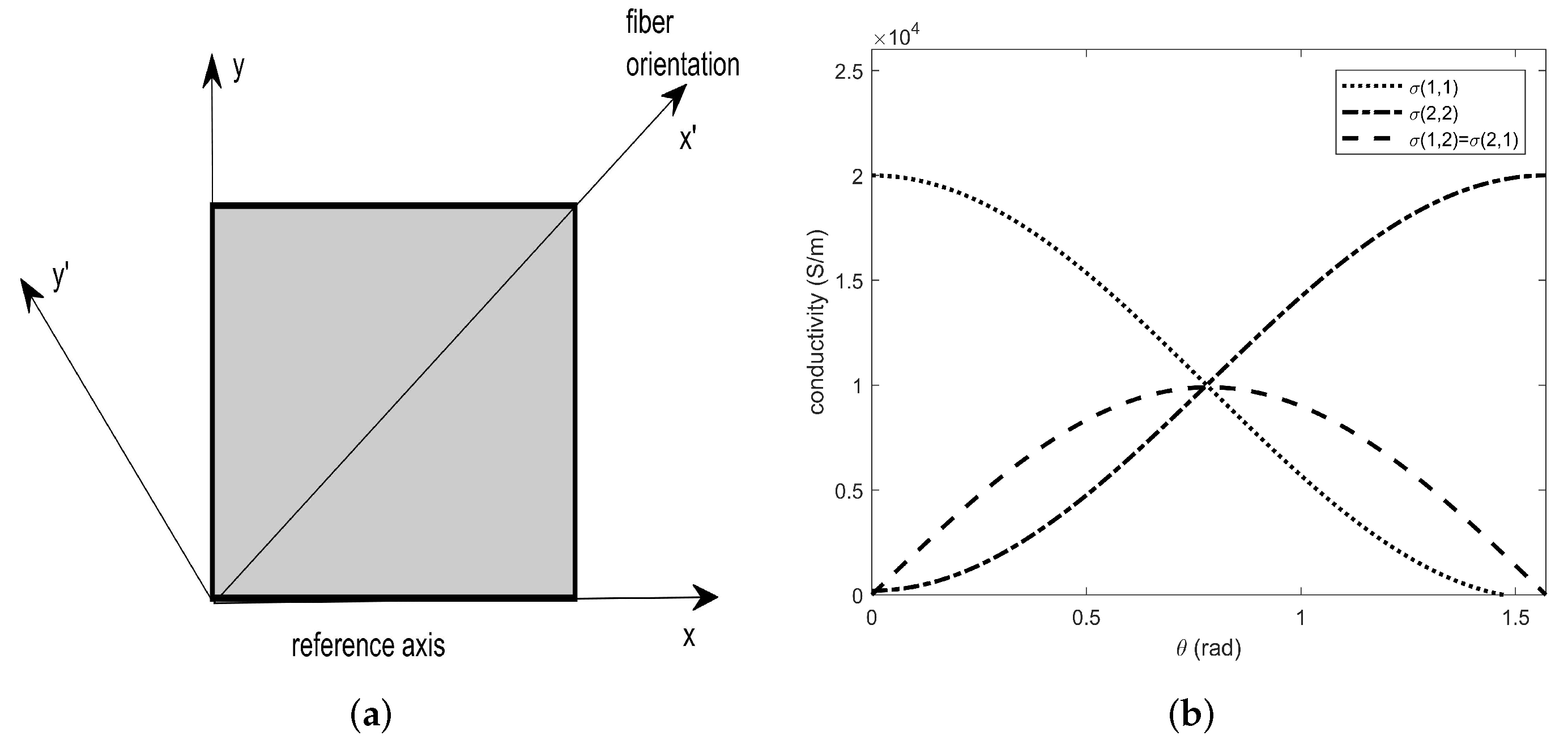
2.1. Electrical Properties of CRFCs
2.2. Existence, Uniqueness and Treatment of Constraints of Irrotationality and Solenoidality of the Numerical Model
2.3. The High-Frequency Numerical Model
2.4. FEM Mesh Generation and Its Quality Assessment
- The index of skewness, which evaluates how equilateral or equiangular the cells are (a value of 0 indicates an equilateral element (best), and a value of 1 indicates an element completely degenerate (worse)).
- An innovative meshing procedure based on the Delaunay triangulation, which has been exploited to obtain a robust mesh (avoiding errors due to the discrepancy with the boundary-boundary elements). The mesh is constructed so that the sphere circumscribed to each finite tetrahedral element inside is devoid of vertices. Furthermore, we observe that the application of the Delaunay triangulation, in our case (non-convex physical system), was carried out by imposing the edges defining the mesh.
2.5. The COMSOL® Multiphysics Implementation of the Numerical Model
3. The EC Maps: Synthetic Generation and Experimental Measurements
3.1. Numerical Simulations
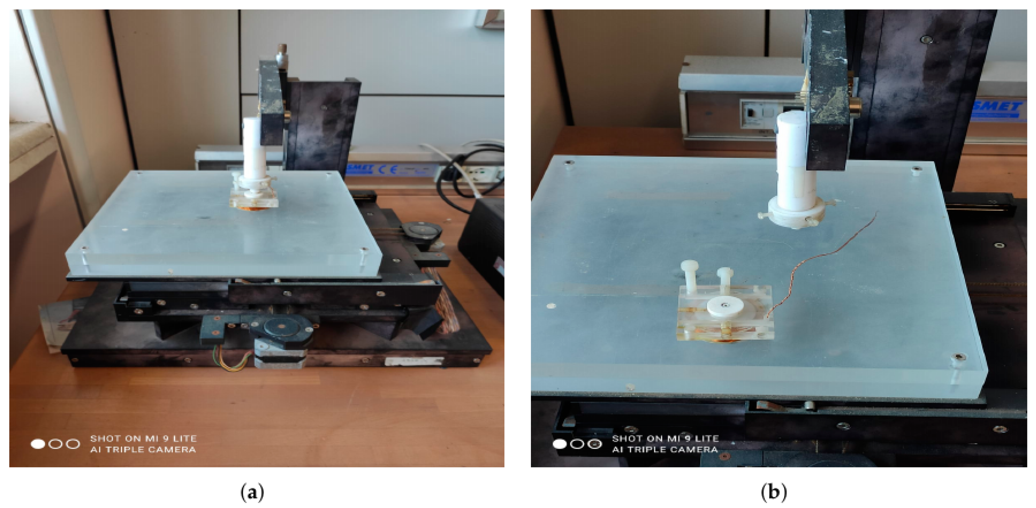
3.2. The Campaign of Measurements
4. Fuzzy Similarity-Based Approach for Defect Classification
4.1. Adaptive Fuzzification of the Maps and Fuzziness Assessment
4.2. F(EC) Maps and Fuzzy Similarities
4.3. Defects in CFRP Plates and Class Constitution
4.4. Fuzzy Procedure for Construction of the EC Maps for Each Class of Defects
5. Results and Discussion
6. Conclusions
Author Contributions
Funding
Institutional Review Board Statement
Informed Consent Statement
Data Availability Statement
Acknowledgments
Conflicts of Interest
Abbreviations
| CFRP | Carbon Fiber-Reinforced Polymers |
| EC | Eddy Current |
| Fuzzy Membership Function | |
| Fuzzy Similarity | |
| Perfect Electric Conductor | |
| Perfect Magnetic Conductor | |
| Electrical Conductivity | |
| Conductivity Along the Fibers | |
| Conductivity Transversal the Fibers | |
| Conductivity Orthogonal the Fibers | |
| Current Density | |
| Electrostatic Field | |
| Rotation Matrix | |
| Magnetic Field | |
| Permeability of the Specimen | |
| j | Imaginary Unit |
| Velocity | |
| Angular Frequency | |
| Scalar Potential | |
| Particular Harmonic Field | |
| Permittivity of the Specimen | |
| External Magnetic Field | |
| External Current Density | |
| Vector Potential | |
| L | Number of Gray Levels |
| Gray Level | |
| FMF | |
| Fuzzy Linear Index | |
| Fuzzy Entropy Index | |
| Fuzzified EC Map | |
| Fuzzy Similarity | |
| Fuzzy Inference Systems |
References
- Park, S.J. Carbon Fiber. In Springer Series in Materials Science; Springer Nature: Basel, Switzerland, 2020. [Google Scholar]
- Hashish, M. Trimming of CFRP Aircraft Components. In Proceedings of the WJTA-IMCA Conference and Expo, Houston, TX, USA, 9–11 September 2013. [Google Scholar]
- Morabito, F.C. Independent Component Analysis and Feature Extraction Techniques for NDT Data. Mater. Eval. 2000, 58, 85–92. [Google Scholar]
- Hashish, M.; Robert, C.; Koutsos, V.; Ray, D. Methods of Modifying Through-Thickness Electrical Conductivity of CFRP for Use in Structural Health Monitoring, and Its Effect on Mechanical Properties—A Review. Manufacturing 2020, 133, 142–149. [Google Scholar]
- Nash, N.H.; Yount, T.M.; McGrail, P.T.; Stanley, W.F. Inclusion of a Thermoplastic Phase to Improve Impact and Post-Impact Performances of Carbon Fibre Reinforced Thermosetting Composite—A Review. Mater Des. 2015, 85, 582–597. [Google Scholar] [CrossRef]
- Senis, E.C.; Glosnoy, I.O.; Dlieu-Barton, J.M.; Thomsen, O.T.; Stanley, W.F. Enhancement of the Electrical and Thermal Properties of Unidirectional Carbon Fibre/epoxy Laminates Through the Addition of Graphene Oxide. J. Mater. Sci. 2019, 54, 8955–8970. [Google Scholar] [CrossRef] [Green Version]
- Kumar, V.; Yokozeki, T.; Okada, T.; Hirano, Y.; Goto, T.; Takahashi, T.; Ogasawara, T. Effect of Through-Thickness Electrical Conductivity of CFRPs on Lightning Strike Damages. Appl. Sci. Manuf. 2019, 114, 429–438. [Google Scholar] [CrossRef]
- Zhou, Y.; Zheng, X.; Xing, F.; Sui, L.; Zheng, Y.; Huang, X. Investigation on the Electrochemical and Mechcanical Performance of CFRP and Steel-Fiber Composite Bar Used for Impressed Current Chathodic Protection Anode. Constrution Build. Mater. 2019, 255, 119377. [Google Scholar] [CrossRef]
- Pellicano, D.; Palamara, I.; Cacciola, M.; Calcagno, S.; Versaci, M.; Morabito, F.C. Fuzzy Similarity Measures for Detection and Classification of Defects in CFRP. IEEE Trans. Ultrason. Ferroelectr. Freq. Control 2013, 60, 1917–1927. [Google Scholar] [CrossRef]
- Li, N.; Li, Y.; Zhou, J.; He, Y.; Hao, X. Delamination and Thermal Damage of Carbon Nanotube/Carbon Fiber Reinforced Epoxy Composites Processed by Microwave Curing. Int. J. Mach. Tools Manuf. 2015, 97, 11–17. [Google Scholar] [CrossRef]
- Domaneschi, M.; Niccolini, G.; Lacidogna, G.; Cimellaro, G.P. Nondestructive Monitoring Techniques for Crack Detection and Localization in RC Elements. Appl. Sci. 2020, 10, 3248. [Google Scholar] [CrossRef]
- Garavaglia, E.; Anzani, A.; Maroldi, F.; Vanerio, F. Non-Invasive Identification of Vulnerability Elements in Existing Buildings and Their Visualization in the BIM Model for Better Project Management: The Case Study of Cuccagna Farmhouse. Appl. Sci. 2020, 10, 2119. [Google Scholar] [CrossRef] [Green Version]
- Kang, D.; Kim, Y.S.; Kim, J.N.; Park, I.K. Characteristics of TiN Thin Films Deposited by Substrate Temperature Variables Using Scanning Acoustic Microscopy. Appl. Sci. 2022, 12, 3571. [Google Scholar] [CrossRef]
- Dattoma, V.; Panella, F.W.; Pirinu, A.; Saponaro, A. Advanced NDT Methods and Data Processing on Industrial CFRP Components. Appl. Sci. 2019, 9, 393. [Google Scholar] [CrossRef] [Green Version]
- Meola, C. Nondestructive Testing in Composite Materials. Appl. Sci. 2020, 10, 5123. [Google Scholar] [CrossRef]
- Gupta, R.; Mitchell, D.; Blanche, J.; Harper, S.; Tang, W.; Pancholi, K.; Baines, L.; Bucknall, D.G.; Flynn, D. A Review of Sensing Technologies for Non-Destructive Evaluation of Structural Composite Materials. J. Compos. Sci. 2021, 5, 319. [Google Scholar] [CrossRef]
- Boccardi, S.; Boffa, N.D.; Carlomagno, G.M.; Del Core, G.; Meola, C.; Monaco, E.; Russo, P.; Simeoli, G. Lock-In Thermography and Ultrasonic Testing of Impacted Basalt Fibers Reinforced Thermoplastic Matrix Composites. Appl. Sci. 2019, 9, 3025. [Google Scholar] [CrossRef] [Green Version]
- Zhu, Q.; Ding, Y.; Tu, D.; Zhang, H.; Peng, Y. Experimental Study of Defect Localization in a Cross-Ply Fiber Reinforced Composite with Diffuse Ultrasonic Waves. Appl. Sci. 2019, 9, 2334. [Google Scholar] [CrossRef] [Green Version]
- Li, H.; Yu, Y.; Li, L.; Liu, B. A Weighted Estimation Algorithm for Enhancing Pulsed Eddy Current Infrared Image in Ecpt Non-Destructive Testing. Appl. Sci. 2019, 9, 4199. [Google Scholar] [CrossRef] [Green Version]
- Tian, L.; Cheng, Y.; Yin, C.; Ding, D.; Song, Y.; Bai, L. Design of the MOI Method Based on the Artificial Neural Network for Crack Detection. Neurocomputing 2017, 226, 80–89. [Google Scholar] [CrossRef]
- Jiao, S.; Li, J.; Du, F.; Sun, L.; Zeng, Z. Characteristics of Eddy Current Distribution in Carbon Fiber Reinforced Polymer. J. Sens. 2016, 2016, 42921234. [Google Scholar] [CrossRef] [Green Version]
- Berger, D.; Lanza, G. Development and Application of Eddy Current Sensor Arrays for Process Integrated Inspection of Carbon Fibre Preforms. Sensors 2018, 18, 4. [Google Scholar] [CrossRef] [Green Version]
- Naidjate, M.; Helifa, B.; Feliachi, M.; Lefkaier, I.K.; Heuer, H.; Schulze, M. A Smart Eddy Current Sensor Dedicated to the Nondestructive Evaluation of Carbon Fibers Reinforced Polymers. Sensors 2017, 17, 1996. [Google Scholar] [CrossRef] [PubMed] [Green Version]
- Katunin, A.; Dragan, K.; Dziendzikowski, M. Identification in Aircraft Composite Structures: A Case Study Using Various Non-Destructive Testing Techniques. Compos. Struct. 2015, 127, 1–9. [Google Scholar] [CrossRef]
- Cacciola, M.; Calcagno, S.; Megali, G.; Pellicanó, D.; Versaci, M. Eddy Current Modeling in Composite Materials. Piers Online 2015, 5, 591–595. [Google Scholar]
- Kanayama, H.; Tagami, D.; Imoto, K.; Sugimoto, S. Finite Element Computation of Magnetic Field Problems with the Displacement Current. J. Comput. Appl. Math. 2003, 159, 77–84. [Google Scholar] [CrossRef] [Green Version]
- Versaci, M.; Jannelli, A.; Morabito, F.C.; Angiulli, G. A Semi-Linear Elliptic Model for a Circular Membrane Mems Device Considering the Effect of the Fringing Field. Sensors 2021, 15, 5237. [Google Scholar] [CrossRef]
- Knibbs, R.H.; Morris, J.B. The Effects of Fibre Orientation on the Physical Properties of Composites. Composites 1974, 5, 209–218. [Google Scholar] [CrossRef]
- Pratap, S.B.; Weldon, W.F. Eddy Currents in Anisotropic Composites Applied to Pulsed Machinery. IEEE Trans. Magn. 1996, 32, 211–223. [Google Scholar] [CrossRef]
- Cheng, D.; Li, Y.; Zhang, J.; Tian, M.; Wang, B.; He, Z.; Dai, L.; Wang, L. Recent Advances in Electrospun Carbon Fiber Electrode for Vanadium Redox Flow Battery: Properties, Structures, and Perspectives. Carbon 2020, 170, 527–542. [Google Scholar] [CrossRef]
- Harrington, R.F. Introduction to Electromagnetic Engineering. In Dover Pubblications; Mineola: New York, NY, USA, 2013. [Google Scholar]
- Alonso Rodriguez, A.; Fernandez, P.; Valli, A. Weak and Strong Formulations for the Time-Harmonic Eddy-Current Problem in General Multi-Connected Domains. Eur. J. Appl. Math. 2003, 14, 387–406. [Google Scholar] [CrossRef]
- Cacciola, M.; Calcagno, S.; Megali, G.; Morabito, F.C.; Pellicano, D.; Versaci, M.F. FEA Design and Misfit Minimization for In-Depth Flaw Characterization in Metallic Plates with Eddy Current Nondestructive Testing. IEEE Trans. Magn. 2009, 45, 1506–1509. [Google Scholar] [CrossRef]
- Alonso Rodriguez, A.; Valli, A. Eddy Current Approximation of Maxwell Equations. COMPEL—Int. J. Comput. Math. Electr. Electron. Eng. 2005, 24, 241–248. [Google Scholar]
- Morisue, T. Magnetic Vector Potential and Electric Scalar Potential in Three-Dimensional Eddy Current Problem. IEEE Trans. Magn. 1982, 18, 531–535. [Google Scholar] [CrossRef]
- Megali, G.; Pellicano, D.; Cacciola, M.; Calcagno, S.; Versaci, M.; Morabito, F.C. EC Modelling and Enhancement Signals in CFRP Inspection. PRogress Electromagn. Res. M 2010, 14, 45–60. [Google Scholar] [CrossRef] [Green Version]
- Biro, O.; Preis, K.; Ticar, I. A FEM Method for Eddy Current Analysis in Laminated Media. In Proceedings of the ISEF 2003, Maribor, Slovenia, 18–20 September 2003. [Google Scholar]
- Versaci, M.; Cutrupi, A.; Palumbo, A. A Magneto-Thermo-Static Study of a Magneto-Rheological Fluid Damper: A Finite Element Analysis. IEEE Trans. Magn. 2020, 57, 4600210. [Google Scholar] [CrossRef]
- Quarteroni, A. Numerical Models For Differential Problems; Springer: Berlin/Heidelberg, Germany, 2015. [Google Scholar]
- Chaira, T.; Ray, A.K. Fuzzy Image Processing and Applications with MATLAB; CRC Press, Taylor & Francis Group: Boca Raton, FL, USA, 2015. [Google Scholar]
- Sridevi, B.; Nadarajan, R. Fuzzy Similarity Measure for Generalized Fuzzy Number. Int. J. Probl. Compt. Math. 2009, 2, 240–253. [Google Scholar]
- Mirhosseini, S.M.; Haghighi, H. Application of the Shuffled Frog Leaping Algorithm (SFLA) in Constructing Fuzzy Classification Systems. Int. J. Comput. Intell. Appl. 2019, 18, 1950019. [Google Scholar] [CrossRef]


| Coil | E-Shaped Core |
|---|---|
| External Diameter: 6 mm | F: 4 mm |
| Internal Diameter: 4 mm | E: 8 mm |
| Height: 2 mm | A: 11 mm |
| Number of Turns: 20 | B: 5.25 mm |
| Lift-Off: 0.005 mm | D: 3.5 mm |
| D′: 1.5 mm | |
| H: 2 mm |
| Class | Radius | Number of EC Maps |
|---|---|---|
| Class #1 | 0.1 mm | 324 |
| Class #2 | 0.2 mm | 332 |
| Class #3 | 0.3 mm | 350 |
| Class #4 | 0.4 mm | 326 |
| Class #5 | 0.5 mm | 329 |
| Class #6 | 0.6 mm | 327 |
| Class #7 | 0.7 mm | 326 |
| Class #8 | 0.8 mm | 329 |
| Class #9 | 0.9 mm | 333 |
| Class #10 | 1 mm | 334 |
| Class ND | without defects | 342 |
| Class | Radius | Number of EC Maps |
|---|---|---|
| Class #1 | 0.1 mm | 198 |
| Class #2 | 0.2 mm | 172 |
| Class #3 | 0.3 mm | 156 |
| Class #4 | 0.4 mm | 164 |
| Class #5 | 0.5 mm | 149 |
| Class #6 | 0.6 mm | 151 |
| Class #7 | 0.7 mm | 157 |
| Class #8 | 0.8 mm | 181 |
| Class #9 | 0.9 mm | 177 |
| Class #10 | 1 mm | 182 |
| Class ND | without defects | 200 |
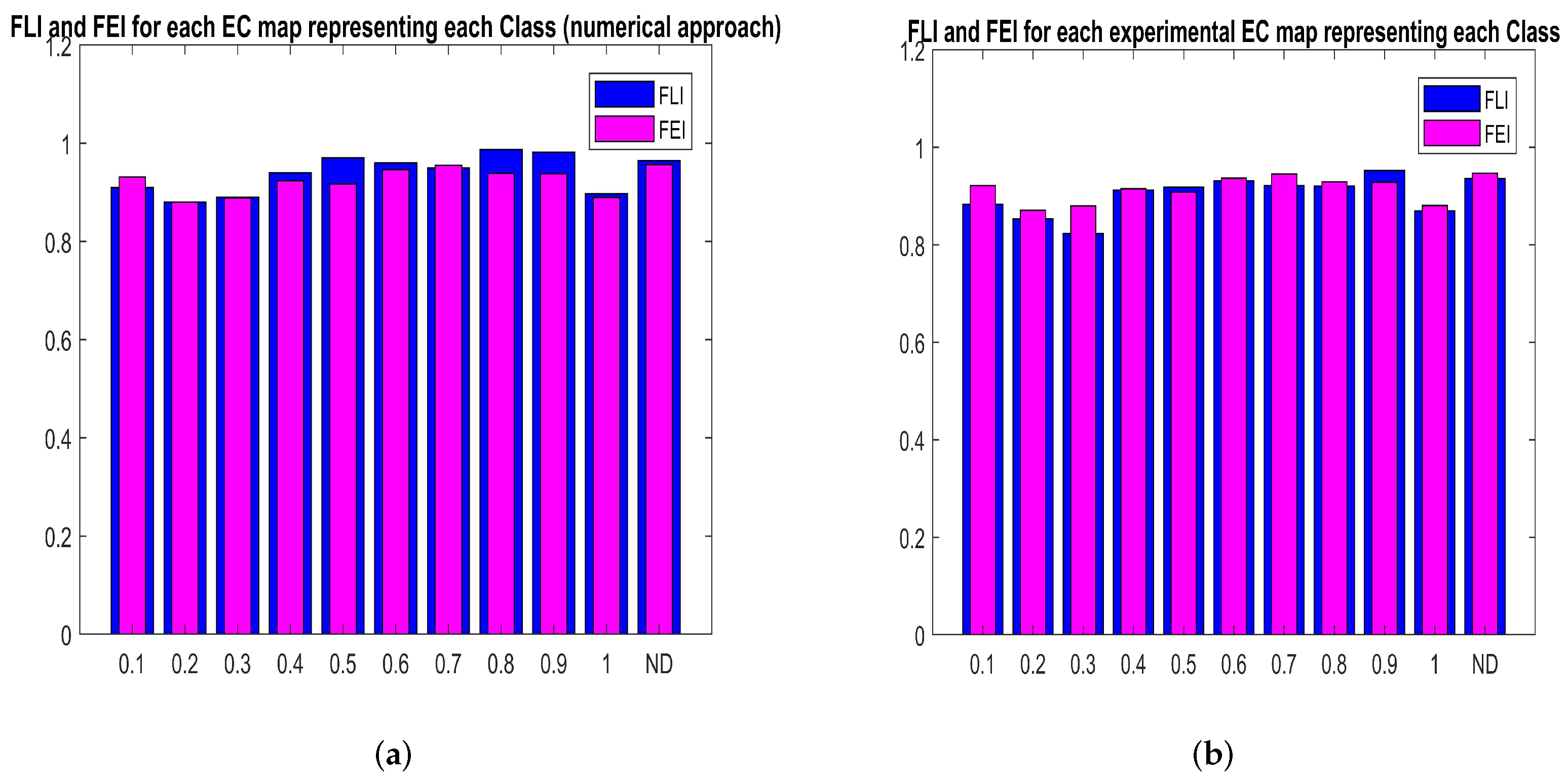
| Class | FLI (num. EC Maps) | FEI (num. EC Maps) | FLI (exp. EC Maps) | FEI (exp. EC Maps) |
|---|---|---|---|---|
| Class 1 | 0.871 ÷ 0.921 | 0.911 ÷ 0.937 | 0.873 ÷ 0.891 | 0.914 ÷ 0.925 |
| Class 2 | 0.872 ÷ 0.899 | 0.862 ÷ 0.892 | 0.851 ÷ 0.864 | 0.865 ÷ 0.881 |
| Class 3 | 0.838 ÷ 0.854 | 0.875 ÷ 0.893 | 0.805 ÷ 0.841 | 0.879 ÷ 0.897 |
| Class 4 | 0.932 ÷ 0.949 | 0.918 ÷ 0.935 | 0.989 ÷ 0.925 | 0.904 ÷ 0.923 |
| Class 5 | 0.925 ÷ 0.956 | 0.989 ÷ 0.923 | 0.896 ÷ 0.923 | 0.887 ÷ 0.914 |
| Class 6 | 0.958 ÷ 0.975 | 0.939 ÷ 0.954 | 0.926 ÷ 0.944 | 0.925 ÷ 0.943 |
| Class 7 | 0.941 ÷ 0.963 | 0.919 ÷ 0.979 | 0.911 ÷ 0.937 | 0.928 ÷ 0.955 |
| Class 8 | 0.939 ÷ 0.952 | 0.926 ÷ 0.941 | 0.878 ÷ 0.933 | 0.901 ÷ 0.932 |
| Class 9 | 0.977 ÷ 0.989 | 0.925 ÷ 0.944 | 0.949 ÷ 0.966 | 0.919 ÷ 0.932 |
| Class 10 | 0.884 ÷ 0.914 | 0.861 ÷ 0.893 | 0.863 ÷ 0.887 | 0.879 ÷ 0.898 |
| Class ND | 0.954 ÷ 0.975 | 0.947 ÷ 0.966 | 0.923 ÷ 0.956 | 0.932 ÷ 0.955 |
| Class | FS1 | FS2 | FS4 | FS4 | FS1 | FS2 | FS3 | FS4 |
|---|---|---|---|---|---|---|---|---|
| Class1 | 0.97 | 0.95 | 0.97 | 0.95 | 0.17 | 0.21 | 0.23 | 0.19 |
| Class 2 | 0.44 | 0.39 | 0.29 | 0.41 | 0.98 | 0.94 | 0.91 | 0.90 |
| Class 3 | 0.11 | 0.12 | 0.21 | 0.19 | 0.15 | 0.19 | 0.17 | 0.23 |
| Class 4 | 0.18 | 0.24 | 0.31 | 0.14 | 0.13 | 0.18 | 0.14 | 0.17 |
| Class 5 | 0.19 | 0.34 | 0.27 | 0.15 | 0.21 | 0.20 | 0.20 | 0.24 |
| Class 6 | 0.14 | 0.14 | 0.19 | 0.18 | 0.18 | 0.17 | 0.16 | 0.11 |
| Class 7 | 0.22 | 0.14 | 0.28 | 0.27 | 0.18 | 0.21 | 0.20 | 0.22 |
| Class 8 | 0.19 | 0.18 | 0.18 | 0.24 | 0.22 | 0.24 | 0.26 | 0.33 |
| Class 9 | 0.11 | 0.09 | 0.18 | 0.07 | 0.18 | 0.33 | 0.35 | 0.36 |
| Class 10 | 0.19 | 0.30 | 0.31 | 0.34 | 0.19 | 0.18 | 0.31 | 0.27 |
| Class ND | 0.18 | 0.17 | 0.14 | 0.22 | 0.19 | 0.24 | 0.25 | 0.29 |
| Class | FS1 | FS2 | FS4 | FS4 | FS1 | FS2 | FS3 | FS4 |
|---|---|---|---|---|---|---|---|---|
| Class1 | 0.15 | 0.26 | 0.19 | 0.31 | 0.24 | 0.22 | 0.17 | 0.12 |
| Class 2 | 0.21 | 0.17 | 0.19 | 0.14 | 0.29 | 0.36 | 0.24 | 0.11 |
| Class 3 | 0.88 | 0.91 | 0.98 | 0.95 | 0.11 | 0.28 | 0.24 | 0.13 |
| Class 4 | 0.21 | 0.23 | 033 | 0.19 | 0.88 | 0.91 | 0.90 | 0.87 |
| Class 5 | 0.24 | 0.22 | 0.14 | 0.13 | 0.19 | 0.22 | 0.18 | 0.31 |
| Class 6 | 0.22 | 0.12 | 0.24 | 0.19 | 0.15 | 0.17 | 0.22 | 0.21 |
| Class 7 | 0.23 | 0.15 | 0.19 | 026 | 0.32 | 0.20 | 0.24 | 0.19 |
| Class 8 | 0.18 | 0.17 | 0.16 | 0.25 | 0.23 | 0.25 | 0.29 | 0.30 |
| Class 9 | 0.21 | 0.18 | 0.36 | 0.11 | 0.24 | 0.31 | 0.34 | 0.30 |
| Class 10 | 0.11 | 0.24 | 0.14 | 0.12 | 0.22 | 0.29 | 0.37 | 0.14 |
| Class ND | 0.12 | 0.15 | 0.14 | 0.20 | 0.18 | 0.23 | 0.28 | 0.25 |
| Class | FS1 | FS2 | FS4 | FS4 | FS1 | FS2 | FS3 | FS4 |
|---|---|---|---|---|---|---|---|---|
| Class1 | 0.21 | 0.22 | 0.37 | 0.21 | 0.33 | 0.14 | 0.22 | 0.18 |
| Class 2 | 0.13 | 0.15 | 0.19 | 0.24 | 0.33 | 0.32 | 0.41 | 0.11 |
| Class 3 | 0.24 | 0.34 | 0.32 | 0.45 | 0.24 | 0.28 | 0.27 | 0.19 |
| Class 4 | 0.25 | 0.32 | 021 | 0.43 | 0.29 | 0.21 | 0.16 | 0.31 |
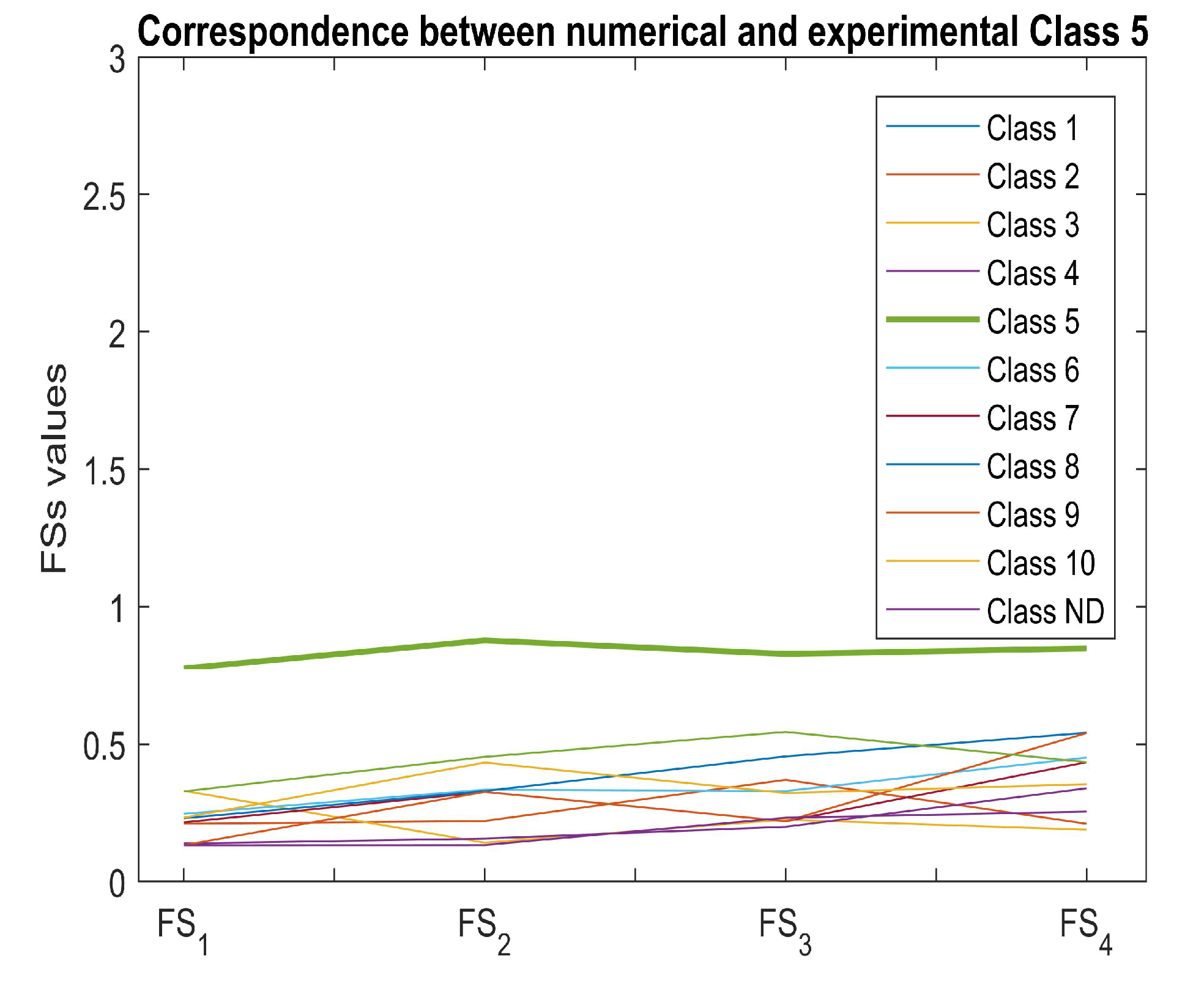
| Class 5 | 0.77 | 0.87 | 0.82 | 0.84 | 0.26 | 0.19 | 0.33 | 0.27 |
| Class 6 | 0.23 | 0.32 | 0.45 | 0.24 | 0.88 | 0.86 | 0.90 | 0.91 |
| Class 7 | 0.13 | 0.32 | 0.21 | 0.54 | 0.27 | 0.25 | 0.26 | 0.28 |
| Class 8 | 0.23 | 0.43 | 0.32 | 0.23 | 0.23 | 0.25 | 0.27 | 0.25 |
| Class 9 | 0.21 | 0.18 | 0.36 | 0.11 | 0.20 | 0.27 | 0.32 | 0.22 |
| Class 10 | 0.13 | 0.13 | 0.23 | 0.25 | 0.21 | 0.27 | 0.35 | 0.12 |
| Class ND | 0.32 | 0.45 | 0.54 | 0.40 | 0.17 | 0.29 | 0.25 | 0.27 |
| Class | FS1 | FS2 | FS4 | FS4 | FS1 | FS2 | FS3 | FS4 |
|---|---|---|---|---|---|---|---|---|
| Class1 | 0.19 | 0.11 | 0.18 | 0.20 | 0.24 | 0.19 | 0.22 | 0.29 |
| Class 2 | 0.12 | 0.16 | 0.15 | 0.31 | 0.29 | 0.24 | 0.34 | 0.22 |
| Class 3 | 0.18 | 0.23 | 0.21 | 0.33 | 0.18 | 0.14 | 0.11 | 0.11 |
| Class 4 | 0.27 | 0.30 | 0.22 | 0.41 | 0.24 | 0.24 | 0.19 | 0.29 |
| Class 5 | 0.21 | 0.17 | 0.13 | 0.12 | 0.13 | 0.18 | 0.24 | 0.227 |
| Class 6 | 0.20 | 0.18 | 0.25 | 0.22 | 0.16 | 0.17 | 0.19 | 0.17 |
| Class 7 | 0.99 | 0.96 | 0.95 | 0.90 | 0.18 | 0.19 | 0.15 | 0.17 |
| Class 8 | 0.40 | 0.41 | 0.37 | 0.33 | 0.97 | 0.88 | 0.91 | 0.90 |
| Class 9 | 0.22 | 0.17 | 0.34 | 0.14 | 0.20 | 0.24 | 0.35 | 0.24 |
| Class 10 | 0.15 | 0.12 | 0.28 | 0.29 | 0.22 | 0.28 | 0.33 | 0.17 |
| Class ND | 0.39 | 0.47 | 0.57 | 0.45 | 0.18 | 0.27 | 0.31 | 0.24 |
| Class | FS1 | FS2 | FS4 | FS4 | FS1 | FS2 | FS3 | FS4 |
|---|---|---|---|---|---|---|---|---|
| Class1 | 0.21 | 0.19 | 0.30 | 0.24 | 0.27 | 0.23 | 0.21 | 0.18 |
| Class 2 | 0.12 | 0.18 | 0.20 | 0.34 | 0.22 | 0.27 | 0.33 | 0.18 |
| Class 3 | 0.17 | 0.25 | 0.30 | 0.34 | 0.28 | 0.24 | 0.22 | 0.27 |
| Class 4 | 0.29 | 0.27 | 0.28 | 0.39 | 0.37 | 0.35 | 0.37 | 0.37 |
| Class 5 | 0.29 | 0.27 | 0.21 | 0.24 | 0.23 | 0.18 | 0.24 | 0.227 |
| Class 6 | 0.20 | 0.18 | 0.25 | 0.22 | 0.16 | 0.17 | 0.19 | 0.17 |
| Class 7 | 0.26 | 0.29 | 0.26 | 0.33 | 0.24 | 0.18 | 0.16 | 0.22 |
| Class 8 | 0.31 | 0.34 | 0.32 | 0.35 | 0.27 | 0.24 | 0.29 | 0.20 |
| Class 9 | 0.91 | 0.94 | 0.95 | 0.93 | 0.16 | 0.25 | 0.24 | 0.19 |
| Class 10 | 0.18 | 0.16 | 0.24 | 0.20 | 0.90 | 0.88 | 0.87 | 0.91 |
| Class ND | 0.21 | 0.12 | 0.40 | 0.35 | 0.25 | 0.21 | 0.37 | 0.27 |
| Class | FS1 | FS2 | FS4 | FS4 |
|---|---|---|---|---|
| Class1 | 0.16 | 0.18 | 0.22 | 0.19 |
| Class 2 | 0.15 | 0.17 | 0.29 | 0.27 |
| Class 3 | 0.28 | 0.22 | 0.27 | 0.24 |
| Class 4 | 0.20 | 0.19 | 0.22 | 0.18 |
| Class 5 | 0.18 | 0.21 | 0.24 | 0.26 |
| Class 6 | 0.17 | 0.19 | 0.22 | 0.21 |
| Class 7 | 0.24 | 0.26 | 0.25 | 0.30 |
| Class 8 | 0.19 | 0.17 | 0.17 | 0.18 |
| Class 9 | 0.11 | 0.12 | 0.16 | 0.16 |
| Class 10 | 0.22 | 0.20 | 0.23 | 0.27 |
| Class ND | 0.97 | 0.91 | 0.94 | 0.90 |
| Approach | Cpu TIME (sec) | Numerical Reconstruction | Experimental Reconstruction |
|---|---|---|---|
| proposed approach | 0.28 | 99.5% | 99.8% |
| -Mamdani | 0.30 | 97.4% | 97.9% |
| -Sugeno | 0.31 | 99.8% | 99.9% |
| fuzzy k-means | 1.22 | 98.6%. | 99.2% |
| SOM | 0.96 | 99.3% | 99.4% |
Publisher’s Note: MDPI stays neutral with regard to jurisdictional claims in published maps and institutional affiliations. |
© 2022 by the authors. Licensee MDPI, Basel, Switzerland. This article is an open access article distributed under the terms and conditions of the Creative Commons Attribution (CC BY) license (https://creativecommons.org/licenses/by/4.0/).
Share and Cite
Versaci, M.; Angiulli, G.; Crucitti, P.; De Carlo, D.; Laganà, F.; Pellicanò, D.; Palumbo, A. A Fuzzy Similarity-Based Approach to Classify Numerically Simulated and Experimentally Detected Carbon Fiber-Reinforced Polymer Plate Defects. Sensors 2022, 22, 4232. https://doi.org/10.3390/s22114232
Versaci M, Angiulli G, Crucitti P, De Carlo D, Laganà F, Pellicanò D, Palumbo A. A Fuzzy Similarity-Based Approach to Classify Numerically Simulated and Experimentally Detected Carbon Fiber-Reinforced Polymer Plate Defects. Sensors. 2022; 22(11):4232. https://doi.org/10.3390/s22114232
Chicago/Turabian StyleVersaci, Mario, Giovanni Angiulli, Paolo Crucitti, Domenico De Carlo, Filippo Laganà, Diego Pellicanò, and Annunziata Palumbo. 2022. "A Fuzzy Similarity-Based Approach to Classify Numerically Simulated and Experimentally Detected Carbon Fiber-Reinforced Polymer Plate Defects" Sensors 22, no. 11: 4232. https://doi.org/10.3390/s22114232