Hybrid Dynamic Traffic Model for Freeway Flow Analysis Using a Switched Reduced-Order Unknown-Input State Observer

 , , ,
, , ,
Abstract
:1. Introduction
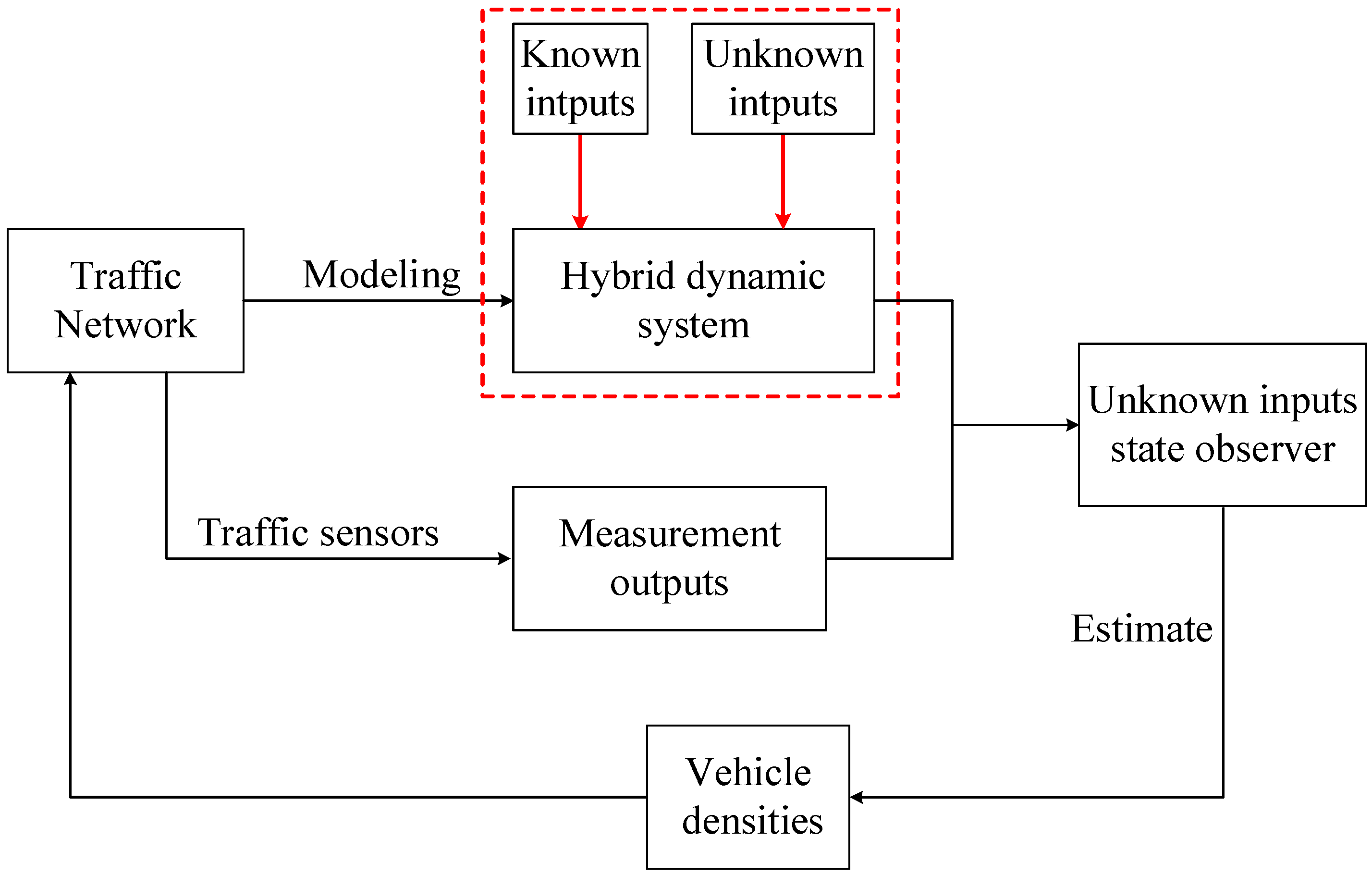
2. Proposed Method
2.1. Hybrid Dynamic System
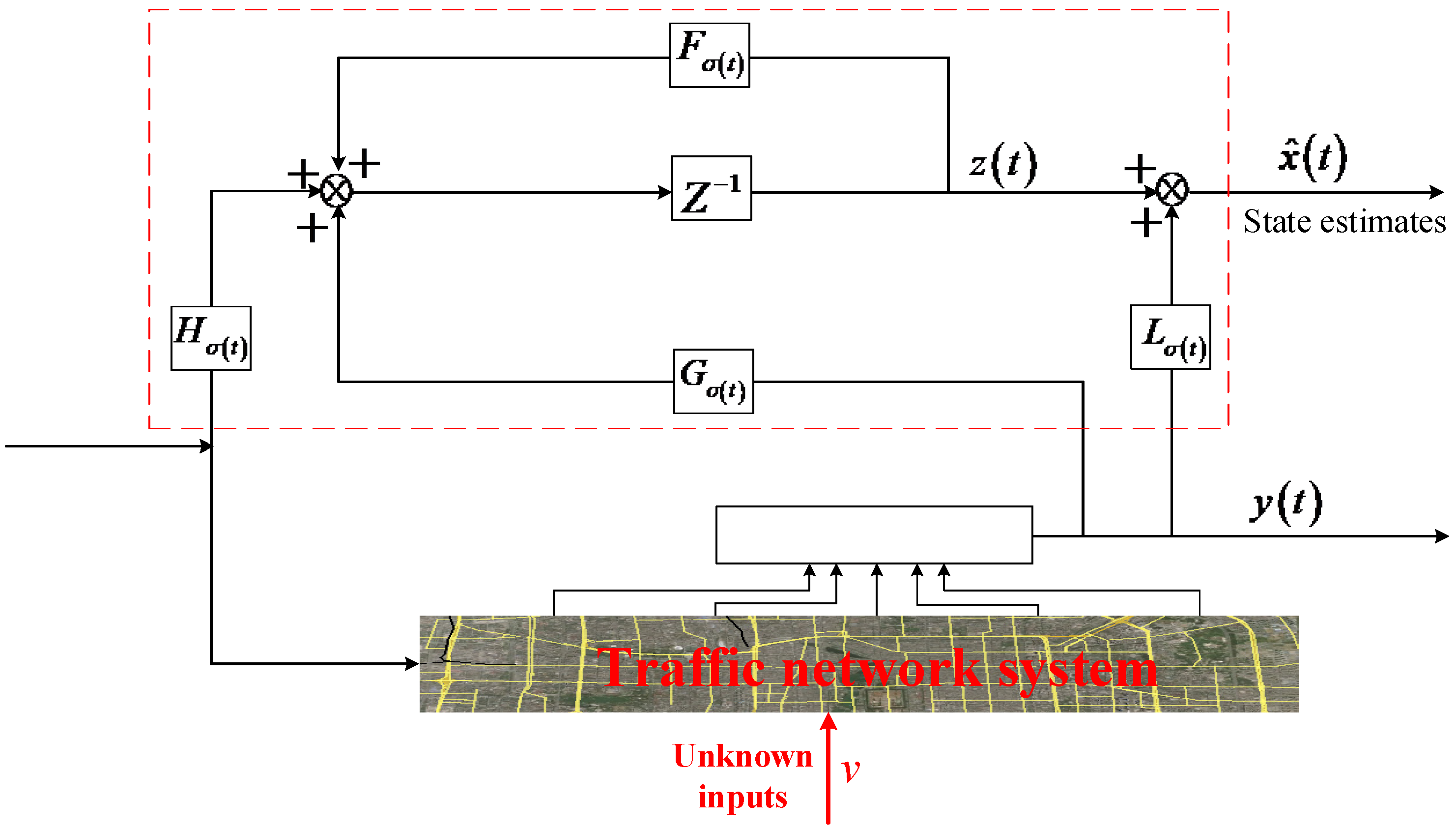
2.2. Unknown-Input State Observer
- (i)
- and .
- (ii)
- The pair is observable or detectable.
- (iii)
- .
2.3. Estimation of Observer Parameters
2.4. Design of the State Observer
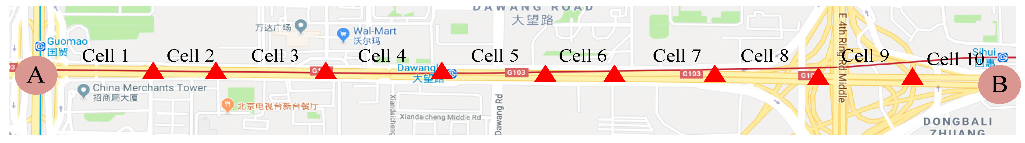
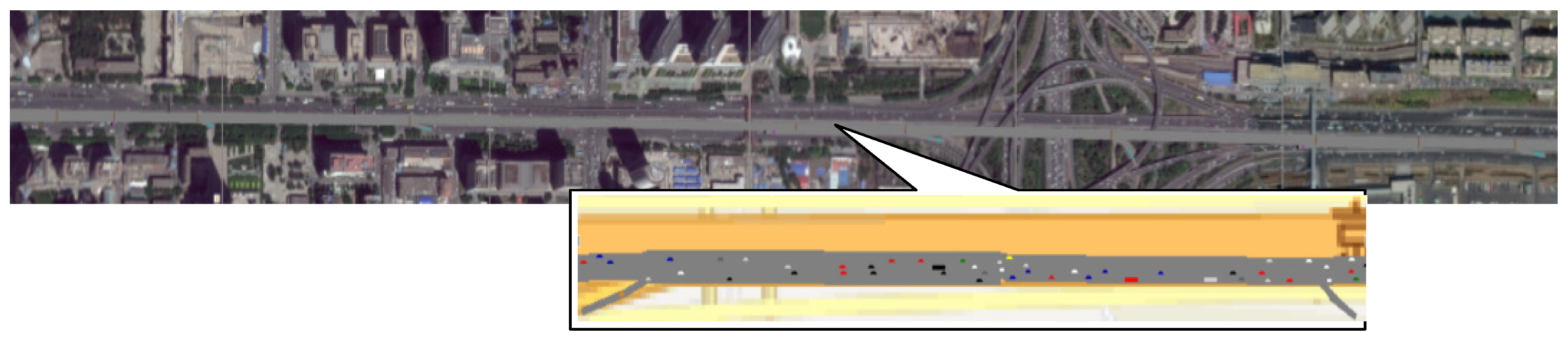
3. Case Study: Beijing Jingtong Freeway
3.1. Data Collection and Processing
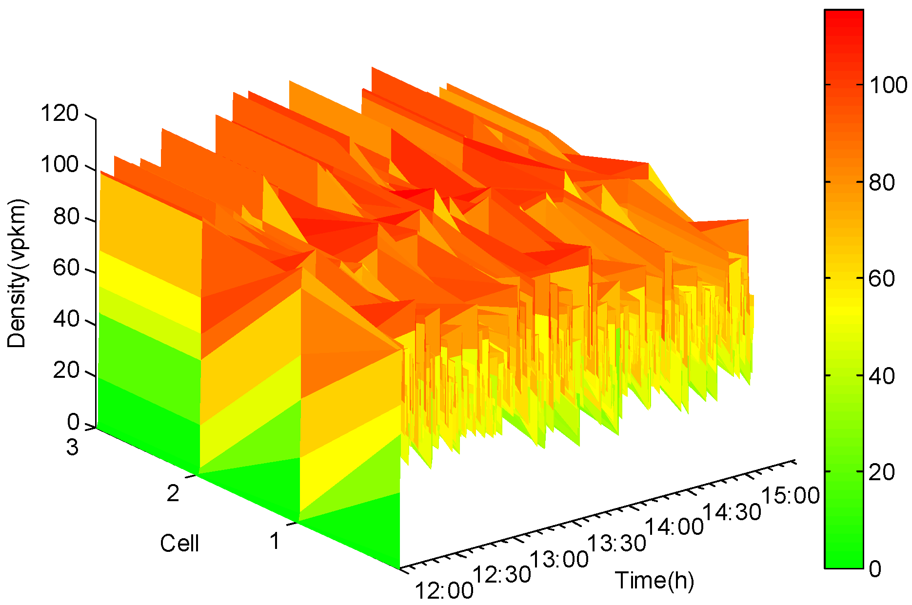
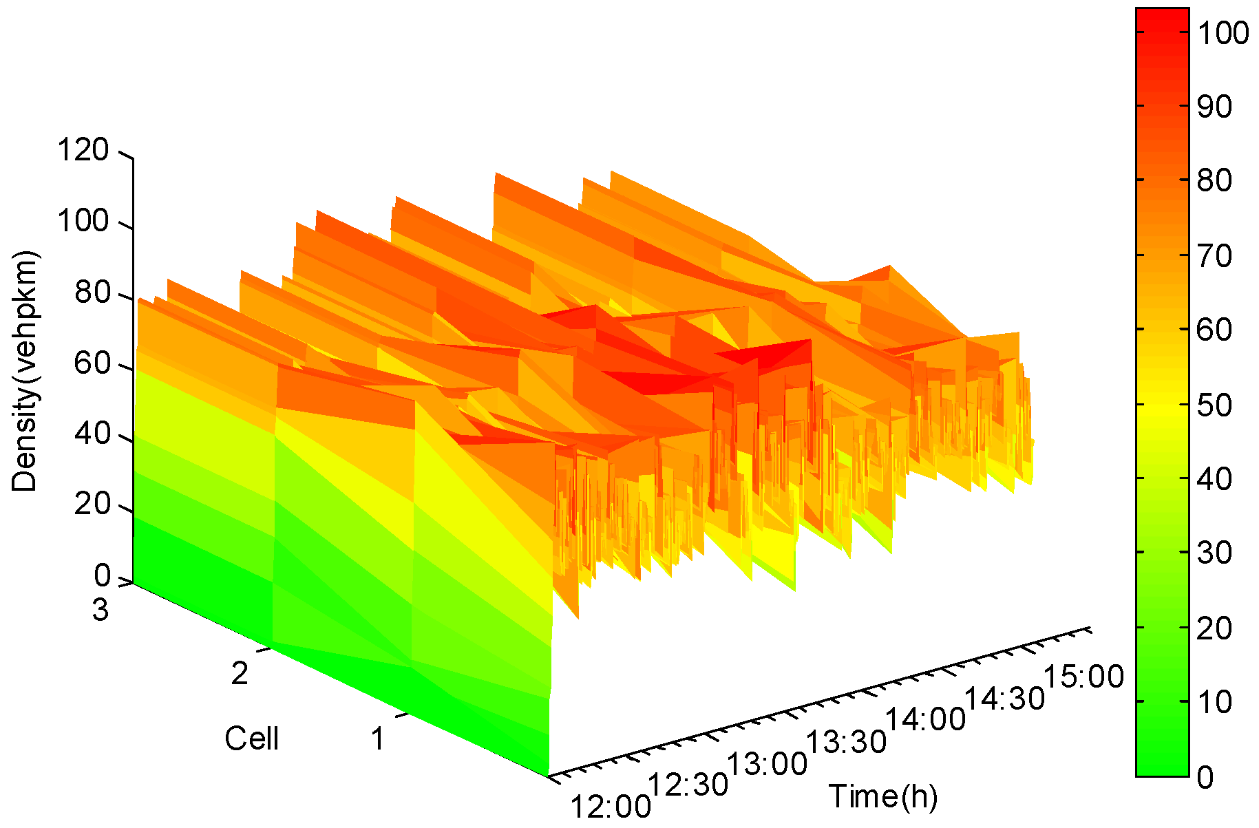
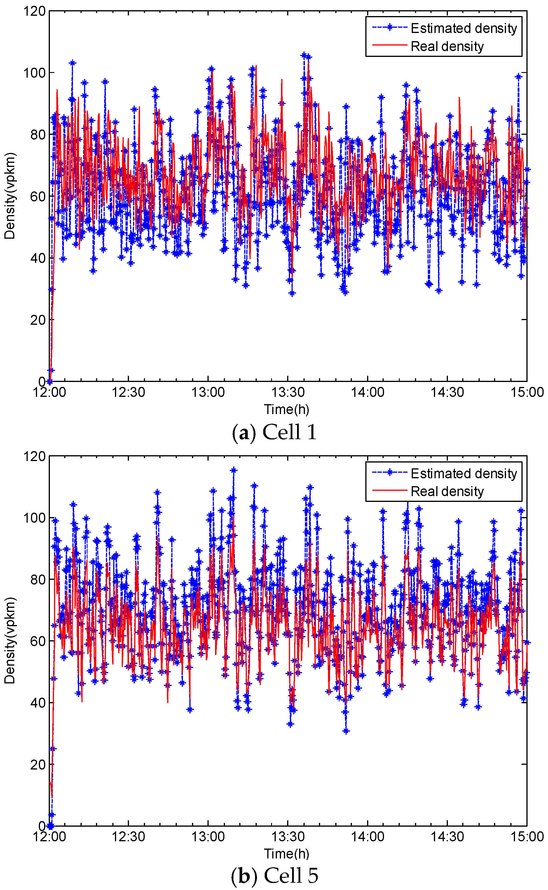
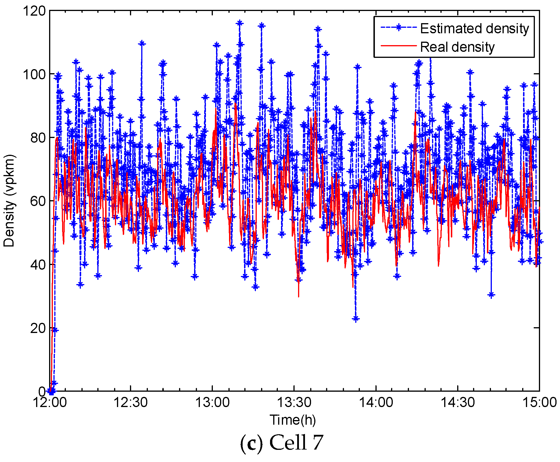
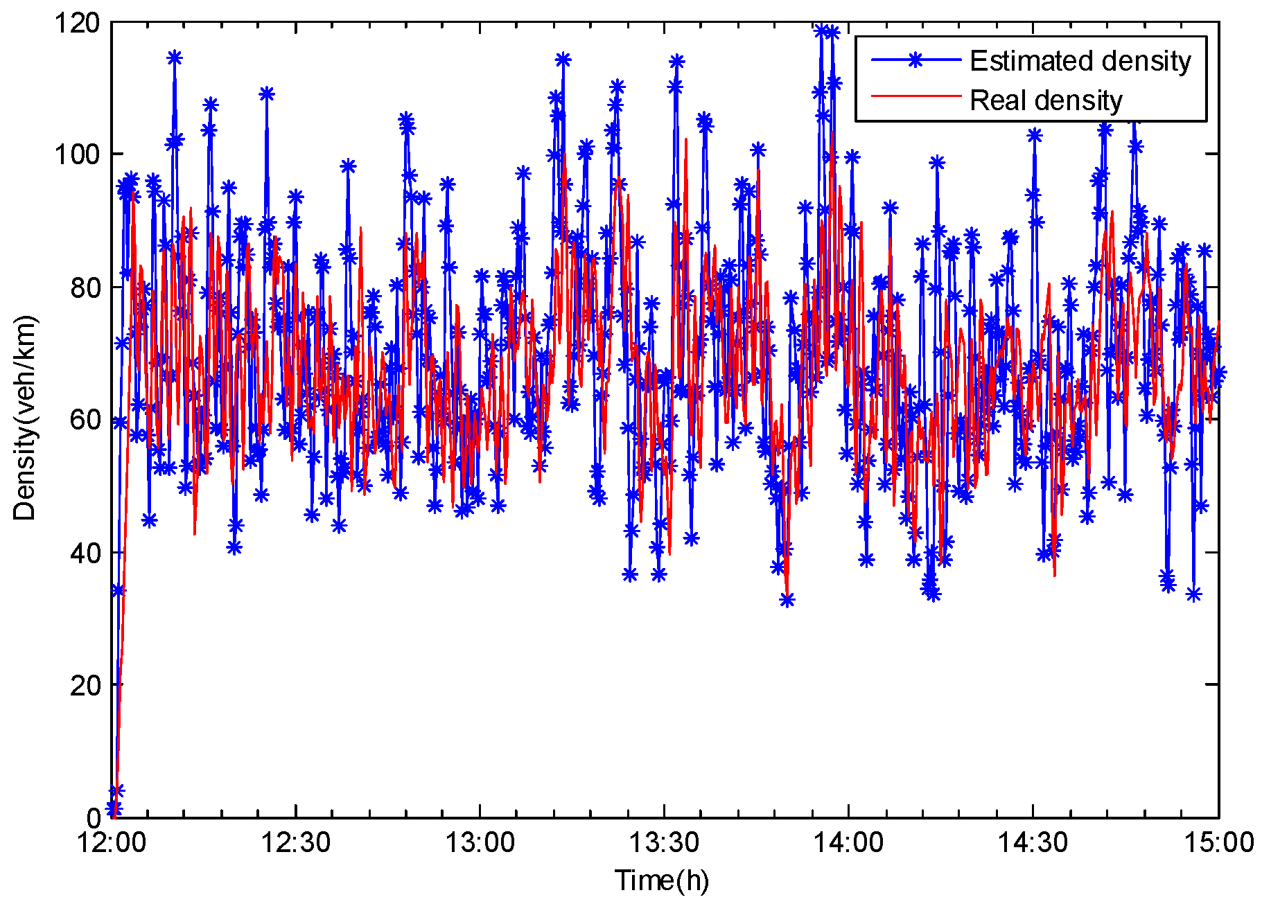
3.2. Analysis Results
4. Conclusions
Author Contributions
Funding
Acknowledgments
Conflicts of Interest
References
- Luenberger, D.G. Observers for multivariable systems. IEEE Trans. Autom. Control 2003, 11, 190–197. [Google Scholar] [CrossRef]
- Luenberger, D.G. An introduction to observers. IEEE Trans. Autom. Control 1971, 16, 596–602. [Google Scholar] [CrossRef]
- Alvarez-Icaza, L.; Munoz, L.; Sun, X.; Horowitz, R. Adaptive observer for traffic density estimation. In Proceedings of the IEEE American Control Conference (ACC), Boston, MA, USA, 30 June–2 July 2004; pp. 2705–2710. [Google Scholar]
- Canudas-de-Wit, C.; Ojeda, L.; Kibangou, A. Graph constrained-CTM observer design for the Grenoble south ring. IFAC Symp. Control Transp. Syst. 2012, 45, 197–202. [Google Scholar] [CrossRef] [Green Version]
- Morbidi, F.; Ojeda, L.; Canudas-de-Wit, C.; Bellicot, I. A new robust approach for highway traffic density estimation. In Proceedings of the European Control Conference (ECC), Strasbourg, France, 24–27 June 2014; pp. 2575–2580. [Google Scholar]
- Vivas, C.; Siri, S.; Ferrara, A. Distributed consensus-based switched observers for freeway traffic density estimation. In Proceedings of the 54th IEEE Decision and Control Conference (CDC), Osaka, Japan, 15–18 December 2015; pp. 3445–3450. [Google Scholar]
- Chen, Y.; Guo, Y.; Wang, Y. Modeling and Density Estimation of an Urban Freeway Network Based on Dynamic Graph Hybrid Automata. Sensors 2017, 17, 716. [Google Scholar] [CrossRef] [PubMed]
- Guo, Y.; Chen, Y.; Zhang, C. Decentralized state-observer-based traffic density estimation of large-scale urban freeway network by dynamic model. Information 2017, 8, 95. [Google Scholar] [CrossRef] [Green Version]
- Guo, Y.; Chen, Y.; Li, W. Traffic density estimation of urban freeway by dynamic model based distributed observer. In Proceedings of the 17th COTA International Conference of Transportation Professionals (CICTP), Shanghai, China, 7–9 July 2017; pp. 603–612. [Google Scholar]
- Guo, Y.; Chen, Y.; Li, W.; Zhang, C. Distributed State-Observer-Based Traffic Density Estimation of Urban Freeway Network. In Proceedings of the 20th IEEE International Conference on Intelligent Transportation Systems (ITSC), Yokohama, Japan, 16–19 October 2017; pp. 1177–1182. [Google Scholar]
- Guo, Y. Dynamic-model-based switched proportional-integral state observer design and traffic density estimation for urban freeway. Eur. J. Control 2018, 44, 103–113. [Google Scholar] [CrossRef]
- Kudva, P.; Viswanadham, N.; Ramakrishna, A. Observers for linear systems with unknown inputs. IEEE Trans. Autom. Control 1980, 25, 113–115. [Google Scholar] [CrossRef]
- Guan, Y.; Saif, M. A Novel Approach to the Design of Unknown Input Observers. IEEE Trans. Autom. Control 1991, 36, 632–635. [Google Scholar] [CrossRef]
- Darouach, M.; Zasadzinski, M.; Xu, S. Full-order observers for linear systems with unknown inputs. IEEE Trans. Autom. Control 1994, 39, 607–609. [Google Scholar] [CrossRef] [Green Version]
- Saif, M. A disturbance accommodating estimator for bilinear systems. In Proceedings of the 1993 IEEE American Control Conference (ACC), San Francisco, CA, USA, 2–4 June 1993; pp. 945–949. [Google Scholar]
- Gao, N.; Darouach, M.; Voos, H. New unified H∞ dynamic observer design for linear systems with unknown inputs. Automatica 2016, 65, 43–52. [Google Scholar] [CrossRef]
- Lungu, M.; Lungu, R. Full-order observer design for linear systems with unknown inputs. Int. J. Control 2012, 85, 1602–1615. [Google Scholar] [CrossRef]
- Bhattacharyya, S. Observer design for linear systems with unknown inputs. IEEE Trans. Autom. Control 1978, 23, 483–484. [Google Scholar] [CrossRef]
- Li, Z.; Guo, Z.; Hu, C.; Li, A. Full-order observers for linear systems with unknown inputs. Comput. Electr. Eng. 2017, 60, 100–115. [Google Scholar]
- Zasadzinski, M.; Rafaralahy, H.; Mechmeche, C.; Darouach, M. On disturbance decoupled observer for a class of bilinear systems. Int. J. Control 1998, 120, 371–377. [Google Scholar] [CrossRef]
- Pertew, A.; Marquez, H.; Zhao, Q. Design of unknown input observers for Lipschitz nonlinear systems. In Proceedings of the 2005 IEEE American Control Conference (ACC), Portland, OR, USA, 8–10 June 2005; pp. 4198–4203. [Google Scholar]
- Seliger, R.; Frank, P. Fault diagnosis by disturbance decoupled nonlinear observers. In Proceedings of the 30th IEEE Conference on Decision and Control (CDC), Brighton, UK, 11–13 December 1991; pp. 2248–2253. [Google Scholar]
- Seliger, R.; Frank, P. Robust component fault detection and isolation in nonlinear dynamic systems using nonlinear unknown input observers. In Proceedings of the IFAC/IMACS Symposium SAFEPROCESS, Baden-Baden, Germany, 10–13 September 1991; pp. 313–318. [Google Scholar]
- Yang, H.; Saif, M. Monitoring and Diagnosis of a Class of Nonlinear Systems Using Nonlinear Unknown Input Observer. In Proceedings of the IEEE Conference on Control Applications, Dearborn, MI, USA; 1996; pp. 1006–1011. [Google Scholar]
- Liu, Y.; Wang, Z.; He, X.; Zhou, D. Observer design for systems with unknown inputs and missing measurements. In Proceedings of the 35th Chinese Control Conference (CCC), Chengdu, China, 27–29 July 2016; pp. 1799–1803. [Google Scholar]
- Sharma, V.; Sharma, B.; Nath, R. Reduced order unknown input observer for discrete time system. In Proceedings of the 2016 IEEE Region 10 Conference (TENCON), Singapore, 22–25 November 2016; pp. 3443–3446. [Google Scholar]
- Mihai, L.; Romulus, L. Reduced Order Observer for Linear Time-Invariant Multivariable Systems with Unknown Inputs. Circuits Syst. Signal Process. 2013, 32, 2883–2898. [Google Scholar]
- Stefen, H.; Stanislaw, H. Observer design for systems with unknown inputs. J. Appl. Math. Comput. Sci. 2005, 15, 431–446. [Google Scholar]
- Lyubchyk, L. Optimal data fusion in decentralized stochastic unknown input observers. In Proceedings of the 7th IEEE International Conference on Intelligent Data Acquisition and Advanced Computing Systems (IDAACS), Berlin, Germany, 12–14 September 2013; pp. 358–362. [Google Scholar]
- Chen, W.; Saif, M. Design of a TS based fuzzy nonlinear unknown input observer with fault diagnosis applications. In Proceedings of the 2007 IEEE American Control Conference, New York, NY, USA, 9–13 July 2007; pp. 2545–2550. [Google Scholar]
- Chen, J.; Patton, R.; Zhang, H. Design of unknown input observers and robust fault detection filters. Int. J. Control 1996, 63, 85–105. [Google Scholar] [CrossRef]
- Gonzalez, J.; Sueur, C. Unknown Input Observer with stability: A Structural Analysis Approach in Bond Graph. Eur. J. Control 2018, 41, 25–43. [Google Scholar] [CrossRef]
- Ifqir, S.; Ichalal, D.; Oufroukh, N.A. Robust interval observer for switched systems with unknown inputs: Application to vehicle dynamics estimation. Eur. J. Control 2018, 44, 3–14. [Google Scholar] [CrossRef]
- Edwards, C.; Chee, P. A Comparison of Sliding Mode and Unknown Input Observers for Fault Reconstruction. Eur. J. Control 2006, 12, 245–260. [Google Scholar] [CrossRef]
- Osoriogordillo, G.; Darouach, M.; Astorgazaragoza, C. H∞ dynamical observers design for linear descriptor systems. Application to state and unknown input estimation. Eur. J. Control 2015, 26, 35–43. [Google Scholar] [CrossRef]
- Zheng, C.; Fan, X.; Wang, C.; Qi, J. GMAN: A Graph Multi-Attention Network for Traffic Prediction. In Proceedings of the Thirty-Fourth Conference on Artificial Intelligence (AAAI 2020), New York, NY, USA, 7–12 February 2020. [Google Scholar]
- Zhang, Y.; Wang, S.; Chen, B.; Cao, J.; Huang, Z. TrafficGAN: Network-Scale Deep Traffic Prediction with Generative Adversarial Nets. IEEE Trans. Intell. Transp. Syst. 2019, 1–12. [Google Scholar] [CrossRef]
- Li, Y.; Shahabi, R.; Yu, C.; Liu, Y. Diffusion Convolutional Recurrent Neural Network:Data-Driven Traffic Forecasting. arXiv 2017, arXiv:1707.01926. [Google Scholar]
- Cao, Z.; Jiang, S.; Zhang, J.; Guo, H. A Unified Framework for Vehicle Rerouting and Traffic Light Control to Reduce Traffic Congestion. IEEE Trans. Intell. Transp. Syst. 2017, 18, 1958–1973. [Google Scholar] [CrossRef]
- Cao, Z.; Guo, H.; Zhang, J.; Fastenrath, U. Multiagent-Based Route Guidance for Increasing the Chance of Arrival on Time. In Proceedings of the Thirtieth AAAI Conference on Artificial Intelligence (AAAI 2016), Phoenix, AZ, USA, 12–17 February 2016; pp. 3817–3820. [Google Scholar]
- Cao, Z.; Guo, H.; Zhang, J. A Multiagent-Based Approach for Vehicle Routing by Considering Both Arriving on Time and Total Travel Time. ACM Trans. Intell. Syst. Technol. 2017, 19, 1–21. [Google Scholar] [CrossRef]
- PTV. VISSIM 5.20 User Manual; Planung Transport Verkeher AG: Karlsruhe, Germany, 2009. [Google Scholar]


| Cell Number | Length (m) | Cell Number | Length (m) |
|---|---|---|---|
| 1 | 300 | 6 | 275 |
| 2 | 160 | 7 | 435 |
| 3 | 460 | 8 | 400 |
| 4 | 430 | 9 | 450 |
| 5 | 400 | 10 | 406 |
| Cell Number | V (km/h) | W (km/h) | C (veh/h) | ||
|---|---|---|---|---|---|
| 1–10 | 65 | 20 | 2800 | 46 | 185 |
© 2020 by the authors. Licensee MDPI, Basel, Switzerland. This article is an open access article distributed under the terms and conditions of the Creative Commons Attribution (CC BY) license (http://creativecommons.org/licenses/by/4.0/).
Share and Cite
Guo, Y.; Li, B.; Christie, M.D.; Li, Z.; Sotelo, M.A.; Ma, Y.; Liu, D.; Li, Z. Hybrid Dynamic Traffic Model for Freeway Flow Analysis Using a Switched Reduced-Order Unknown-Input State Observer. Sensors 2020, 20, 1609. https://doi.org/10.3390/s20061609
Guo Y, Li B, Christie MD, Li Z, Sotelo MA, Ma Y, Liu D, Li Z. Hybrid Dynamic Traffic Model for Freeway Flow Analysis Using a Switched Reduced-Order Unknown-Input State Observer. Sensors. 2020; 20(6):1609. https://doi.org/10.3390/s20061609
Chicago/Turabian StyleGuo, Yuqi, Bin Li, Matthew Daniel Christie, Zongzhi Li, Miguel Angel Sotelo, Yulin Ma, Dongmei Liu, and Zhixiong Li. 2020. "Hybrid Dynamic Traffic Model for Freeway Flow Analysis Using a Switched Reduced-Order Unknown-Input State Observer" Sensors 20, no. 6: 1609. https://doi.org/10.3390/s20061609