Geometric Aberration Theory of Offner Imaging Spectrometers

Abstract

A third-order aberration theory has been developed for the Offner imaging spectrometer comprising an extended source; two concave mirrors; a convex diffraction grating; and an image plane. Analytic formulas of the spot diagram are derived for tracing rays through the system based on Fermat’s principle. The proposed theory can be used to discuss in detail individual aberrations of the system such as coma, spherical aberration and astigmatism, and distortion together with the focal conditions. It has been critically evaluated as well in a comparison with exact ray tracing constructed using the commercial software ZEMAX. In regard to the analytic formulas, the results show a high degree of practicality.

1. Introduction

An imaging spectrometer can provide a simultaneous collection of spatial and spectral information of targets with high resolution [1]. Currently, spectrometers have become an indispensable part of many fields including satellite remote sensing, space exploration, security, environment assessment, resource detection, agriculture, medicine, manufacturing, oceanography, and ecology [2,3,4,5,6].

The recent trend in imaging spectrometers is toward a simple set-up and a very compact configuration with high optical performance over the whole spectral range of the system [7]. This can be observed in the Offner imaging spectrometer with a concentric structure, using spherical optics. This spectrometer is obtained by replacing the convex secondary mirror of the Offner imaging system with a reflective convex diffraction grating [8]. It provides a high signal-to-noise ratio and small spot sizes together with low spatial and spectral distortions [7,8,9,10,11]. Because diffraction occurs at the grating, the perfect symmetry of the concentric configuration is altered, thereby increasing for example the coma and astigmatism. Although good optical performance is maintained with the rapid development of imaging spectrometers; more improvements need to be achieved to meet the dual demands for higher spatial and spectral resolution.

There have been various attempts to optimize and design an aberration-correct Offner imaging spectrometer. In 1999, Chrisp split the concave mirror into two concentric mirrors of different radii, increasing the degrees-of-freedom of the system designs [12]. By changing the off-axis parameters, tilting or decentering some elements, and making appropriate adjustments to the radii of the two spherical mirrors, the optical quality of the system was optimized. In 2001, Xiang and Mikes proposed an aberration-corrected spectrometer that included a convex diffraction grating having a number of nonparallel lines [13]. They believed the curves of the convex grating provided the correction for field aberrations. However, forming such a convex grating is difficult with the existing technology and theory. In 2006, Prieto-Blanco and coworkers presented an approach based on the calculation of both the meridional and the sagittal images of an off-axis object point [5]. Making the meridional and sagittal curves tangent to each other for a given wavelength results in a decrease in astigmatism. In 2007, Robert analyzed the out-of-plane dispersion in an Offner spectrometer. When the dispersion is perpendicular to the meridional plane, better performance is obtained for the system with a short entrance slit [14]. In 2014, Prieto-Blanco and coworkers proposed a Wynne-Offner layout consisting of a concave mirror and a concentric meniscus lens that included a diffraction grating at the center of one of its surfaces [15,16,17,18]. All the above methods have described the effect of aberrations such as astigmatism on the optical quality of the Offner spectrometer and how to optimize the system. However, these methods are relatively singular-use solutions and are not widely used in developing a system for different requirements [19,20].

In this paper, we propose a third-order geometric aberration theory of the Offner imaging spectrometer to provide an alternative aberration-correction method. This method is an extension and new application of Namioka’s theories [21,22,23,24,25,26]. Namioka and his team have shown aberration theories based on the light path function for a single grating or a double-element system that can correctly describe the individual aberrations and can be used to design an advanced optical system. Taking an extended source into consideration, analytic formulas of the spot diagram and the individual aberrations are derived for tracing rays through the system based on Fermat’s principle and Namioka’s theories. With these formulas, aberrations including coma, aberration, astigmatism, and distortion of the three-concentric-element (Offner) configuration are discussed in detail together with focal conditions. Finally, the theory is critically evaluated in a comparison with exact ray tracing constructed using the commercial software ZEMAX (Zemax software development company, bellevue, WS, USA). The results indicate a high degree of validity of the analytic formulas.

2. Three-Concentric-Element (Offner) Optical System

We consider an Offner optical system that comprises a planar light source S, two concave mirrors M₁ and M₂, a convex diffraction grating G, and an image plane Σ (Figure 1). In this system, the elements are arranged in such a way that the normal axes to S at A₀, to M₁ at O₁, to G at O, and to M₂ at O₂ lie in a common plane called the meridional plane. The incident principal ray A₀O₁ is reflected by M₁ toward O, and the reflected principal ray O₁O of wavelength λ in the m₁th order is diffracted by G toward O₂. The diffracted principal ray OO₂ is then further reflected by M₂. This reflected principal ray of λ meets Σ at a point B₀, which lies in the meridional plane as well. Here we assume that the principal ray of wavelength λ is designed to end up in the center of the image plane Σ; and we assume that the image plane Σ is perpendicular both to the reflected principal ray O₂B₀ and to the meridional plane as well. The distances A₀O₁, O₁O, OO₂, and O₂B₀ are denoted by r₁, r, r′, and r₂, respectively.

For convenience, we introduce five rectangular coordinate systems attached to S, M₁, G, M₂, and Σ (Figure 1). The origins are at A₀, O₁, O, O₂, and B₀, the X_S, x₁, x, x₂, and X axes are the normal axes of the respective elements, and the Y_S, y₁, y, y₂, and Y axes lie in the meridional plane. A general ray originating from a source point A in S is reflected at a point Q₁ on the surface of M₁. The reflected ray meets G at a point P on the nth groove of G, and the diffracted ray of wavelength λ in m-th order meets M₂ at a point Q₂. The outgoing ray of wavelength λ from Q₂ intersects Σ at a point B, forming a spot in the image plane Σ. We designate the coordinates of A, Q₁, P, Q₂, and B by (0, s, z), (ξ₁, ω₁, l₁), (ξ, ω, l), (ξ₂, ω₂, l₂), and (0, Y, Z) in the X_SY_SZ_S, x₁y₁z₁, xyz, x₂y₂z₂, and XYZ systems, respectively, and those of A and B as well by (x₁, y₁, z₁) and (x₂, y₂, z₂) in the x₁y₁z₁ and x₂y₂z₂ system, separately. Here, x₁ and y₁ are expressed as

$$x_1={\mathrm{r}}_1\cos {\mathsf{\theta }}_1+s\sin {\mathsf{\theta }}_1,y_1={\mathrm{r}}_1\sin {\mathsf{\theta }}_1-s\cos {\mathsf{\theta }}_1.$$

(1)

We assume as well that the zeroth groove of G passes through O, and that the groove number n is positive or negative according to whether the n-th groove passes through the y-axis on its positive or negative side. The groove number n of G expressed in a power series of ω and l is given as [26]:

$$n{\mathsf{\lambda }}_0=n_{10}\mathsf{\omega }+\frac{1}{2}(n_{20}{\mathsf{\omega }}^2+n_{02}{l}^2+n_{30}{\mathsf{\omega }}^3+n_{12}\mathsf{\omega }{l}^2)+\frac{1}{8}(n_{40}{\mathsf{\omega }}^4+2n_{22}{\mathsf{\omega }}^2{l}^2+n_{04}{l}^4)+\dots ,$$

(2)

where λ₀ is the recording wavelength of G.

In this system shown in Figure 1, both the concave mirrors M₁ and M₂ and the convex grating G are spherical in shape. The corresponding mathematical expression of the surface figure of M_i (or G) is given by

$${({\mathsf{\xi }}_i-R_i)}^2+{\mathsf{\omega }}_i{}^2+l_i{}^2=R_i{}^2,$$

(3)

where R_i (i = 1, 2 for M₁ and M₂, no suffix for G) is the radius of M_i or G. Equation (3) expanded as a power series of ω_i and l_i is:

$${\mathsf{\xi }}_i=\frac{1}{2R_i}{\mathsf{\omega }}_i^2+\frac{1}{2R_i}{l}_i^2+\frac{1}{8R_i^3}{\mathsf{\omega }}_i^4+\frac{1}{4R_i^3}{\mathsf{\omega }}_i^2{l}_i^2+\frac{1}{8R_i^3}{l}_i^4+O(\frac{{\mathsf{\omega }}_i^6}{R_i^3}).$$

(4)

The angles of incidence θ_i and reflection/diffraction θ_i′ of the principal ray at the vertices of M_i (or G) are considered as positive or negative depending on whether the relevant principal ray lies in the first or fourth quadrant of the x_iy_iz_i coordinate system. The angles θ and θ′ are related through the grating equation,

$$\mathsf{\sigma }(\sin \mathsf{\theta }+\sin {\mathsf{\theta }}^{\prime })=\mathrm{m}\mathsf{\lambda },$$

(5)

where σ is the effective grating constant obtained by:

$$\mathsf{\sigma }\equiv {1/\left(\partial n/\partial \mathsf{\omega }\right)}_{\mathsf{\omega }=l=0}={\mathsf{\lambda }}_0/n_{10},$$

(6)

which can be referred to [26].

3. Ray-Tracing Formulas

First, we denote the distances AQ₁, Q₁P, PQ₂, and Q₂B by q₁, p₁, q₂, and p₂, respectively. According to Namioka’s theory, the application of Fermat’s principle to the light-path function for M_i,

$$F_{M_i}=q_i+p_i,$$

(7)

yields the direction cosines (L_i′, M_i′, N_i′) of the reflected ray p_i in terms of the direction cosines (L_i, M_i, N_i) of the incident ray q_i and given system parameters:

$$\begin{array}{l}{L^{\prime }}_i=L_i+{\mathsf{\tau }}_i,\\ {M^{\prime }}_i=M_i-{\mathsf{\tau }}_i\left(\frac{\partial {\mathsf{\xi }}_i}{\partial {\mathsf{\omega }}_i}\right),\\ {N^{\prime }}_i=N_i-{\mathsf{\tau }}_i\left(\frac{\partial {\mathsf{\xi }}_i}{\partial l_i}\right).\end{array}$$

(8)

where all the quantities are defined in the x_iy_iz_i coordinate system. In Equation (8), we have

$${\mathsf{\tau }}_i=\frac{2[-L_i+M_i(\partial {\mathsf{\xi }}_i/\partial {\mathsf{\omega }}_i)+N_i(\partial {\mathsf{\xi }}_i/\partial l_i)]}{1+{(\partial {\mathsf{\xi }}_i/\partial {\mathsf{\omega }}_i)}^2+{(\partial {\mathsf{\xi }}_i/\partial l_i)}^2},$$

(9)

where i = 1, 2 for M₁ and M₂. L_i, M_i, and N_i are obtained from the definition of the direction cosines of the incident ray q_i.

The intersecting point P (ξ, ω, l) is determined by solving simultaneously the equation of the ray Q₁P in the xyz coordinate system

$$\frac{\mathsf{\xi }-{\overline{\mathsf{\xi }}}_1}{L}=\frac{\mathsf{\omega }-{\overline{\mathsf{\omega }}}_1}{M}=\frac{l-{\overline{l}}_1}{N},$$

(10)

and Equation (3) with i = 1. In Equation (10) (${\overline{\mathsf{\xi }}}_1$, ${\overline{\mathsf{\omega }}}_1$₁, ${\overline{\mathrm{l}}}_1$) and (L, M, N) are the coordinates of the point Q₁ and the direction cosines of the ray Q₁P, which are both defined in the xyz coordinate system. They are obtained by applying proper coordinate transformations to (ξ₁, ω₁, l₁) and (L₁′, M₁′, N₁′).

Different from the above calculation for M_i, the application of Fermat’s principle to the light-path function for G,

$$F=p_1+q_2+nm\mathsf{\lambda },$$

(11)

yields the direction cosines (L′, M′, N′) of the diffracted ray PQ₂ in terms of the direction cosines (L, M, N) of the incident ray Q₁P and given system parameters:

$$\begin{array}{l}{L}^{\prime }=L+\mathsf{\tau },\\ M^{\prime }=M+m\mathsf{\lambda }\left(\frac{\partial n}{\partial \mathsf{\omega }}\right)-\mathsf{\tau }\left(\frac{\partial \mathsf{\xi }}{\partial \mathsf{\omega }}\right),\\ N^{\prime }=N+m\mathsf{\lambda }\left(\frac{\partial n}{\partial l}\right)-\mathsf{\tau }\left(\frac{\partial \mathsf{\xi }}{\partial l}\right).\end{array}$$

(12)

where all the quantities are defined in the xyz coordinate system. In Equation (12), we have

$$\begin{array}{l}\mathsf{\tau }=\frac{1}{\mathsf{\rho }}\left(\mathsf{\nu }+\sqrt{{\mathsf{\nu }}^2-\mathsf{\kappa }\mathsf{\rho }}\right),\\ \mathsf{\rho }=1+{\left(\frac{\partial \mathsf{\xi }}{\partial \mathsf{\omega }}\right)}^2+{\left(\frac{\partial \mathsf{\xi }}{\partial l}\right)}^2,\\ \mathsf{\nu }=-L+\left(M+m\mathsf{\lambda }\frac{\partial n}{\partial \mathsf{\omega }}\right)\frac{\partial \mathsf{\xi }}{\partial \mathsf{\omega }}+\left(N+m\mathsf{\lambda }\frac{\partial n}{\partial l}\right)\frac{\partial \mathsf{\xi }}{\partial l},\\ \mathsf{\kappa }=2m\mathsf{\lambda }\left(M\frac{\partial n}{\partial \mathsf{\omega }}+N\frac{\partial n}{\partial l}\right)+{\left(m\mathsf{\lambda }\right)}^2\left[{\left(\frac{\partial n}{\partial \mathsf{\omega }}\right)}^2+{\left(\frac{\partial n}{\partial l}\right)}^2\right].\end{array}$$

(13)

The intersecting point Q₂ (ξ₂, ω₂, l₂) is determined by solving simultaneously Equation (3) with i = 2 and the equation of ray PQ₂ in the x₂y₂z₂ coordinate system,

$$\frac{{\mathsf{\xi }}_2-\overline{\mathsf{\xi }}}{L_2}=\frac{{\mathsf{\omega }}_2-\overline{\mathsf{\omega }}}{M_2}=\frac{l_2-\overline{l}}{N_2},$$

(14)

where ($\overline{\mathsf{\xi }}$, $\overline{\mathsf{\omega }}$, $\overline{\mathrm{l}}$) and (L₂, M₂, N₂) are the coordinates of point P and the direction cosines of ray PQ₂, both defined in the x₂y₂z₂ coordinate system. They are obtained by applying proper coordinate transformations to (ξ, ω, l) and (L′, M′, N′).

The image plane Σ is expressed in the x₂y₂z₂ coordinate system as

$$x_2\cos {{\mathsf{\theta }}^{\prime }}_2+y_2\sin {{\mathsf{\theta }}^{\prime }}_2=r_2.$$

(15)

Then, the intersection B of the reflected ray Q₂B with the image plane Σ is determined by solving the equation of the ray Q₂B in the x

₂y₂z₂ coordinate system,

$$\frac{x_2-{\mathsf{\xi }}_2}{{L^{\prime }}_2}=\frac{y_2-{\mathsf{\omega }}_2}{{M^{\prime }}_2}=\frac{z_2-l_2}{{N^{\prime }}_2},$$

(16)

from which we obtain:

$$x_2={\mathsf{\xi }}_2+p_2{L^{\prime }}_2,y_2={\mathsf{\omega }}_2+p_2{M^{\prime }}_2,z_2=l_2+p_2{N^{\prime }}_2.$$

(17)

By applying proper coordinate transformations to B (x₂, y₂, z₂), the ray-traced spot B (0, Y, Z) in the XYZ coordinate system is expressed as

$$Y=\left(r_2\sin {{\mathsf{\theta }}^{\prime }}_2-y_2\right)\sec {{\mathsf{\theta }}^{\prime }}_2,\text{\hspace{0.17em}\hspace{0.17em}\hspace{0.17em}\hspace{0.17em}}Z=z_2.$$

(18)

All the above equations presented in this section provide a complete set of ray-tracing formulas.

4. Analytic Expression of Spot Diagrams and Aberrations

The imaging characteristics of the three-concentric-element optical system may be analyzed numerically using ray tracing. Although ray tracing provides accurate spot diagrams with comparative ease, it lacks the ability to give explicit analytical expressions for the focal condition and individual aberrations of the system under consideration. According to Namioka’s theory, we express the relationship between the coordinates of a source point and its image by expanding the ray-tracing formulas given in Section 3 into power series of ω₁, l₁, and the coordinates of A₀ in the X_SY_SZ_S system. In this way—although laborious—a third-order aberration theory is developed for the system, which has a high degree of validity.

Taking the expansion of the coordinates of point P as an example, we determine its position in the xyz coordinate system by finding the intersection of ray Q₁P with the grating blank surface. We express ω and l in a power series of ω₁^hl₁ⁱz^js^k (h + i + j + k ≤ 3) under assumptions of:

$$\mathsf{\omega }={\displaystyle \sum _{h+i+j+k=1}^3{A}_{hijk}}{\mathsf{\omega }}_1^h{l}_1^i{z}^j{s}^k,l={\displaystyle \sum _{h+i+j+k=1}^3{B}_{hijk}}{\mathsf{\omega }}_1^h{l}_1^i{z}^j{s}^k.$$

(19)

To determine ω and l, we derive first the direction cosines (L, M, N) as power series of ω₁, l₁, s and z by expanding their definitions:

$$L=\frac{\mathsf{\xi }-{\overline{\mathsf{\xi }}}_1}{p_1},M=\frac{\mathsf{\omega }-{\overline{\mathsf{\omega }}}_1}{p_1},N=\frac{l-{\overline{l}}_1}{p_1},$$

(20)

as

$$\begin{array}{l}L={\displaystyle \sum _{h+i+j+k=1}^3{\left(H_{hijk}\right)}_L}{\mathsf{\omega }}_1^h{l}_1^i{z}^j{s}^k,\\ M={\displaystyle \sum _{h+i+j+k=1}^3{\left(H_{hijk}\right)}_M}{\mathsf{\omega }}_1^h{l}_1^i{z}^j{s}^k,\\ N={\displaystyle \sum _{h+i+j+k=1}^3{\left(H_{hijk}\right)}_N}{\mathsf{\omega }}_1^h{l}_1^i{z}^j{s}^k.\end{array}$$

(21)

where coefficients (H_hijk)_L, (H_hijk)_M, and (H_hijk)_N are functions of R₁, r, θ₁, and θ only.

Next, we adopt another approach to expand the direction cosines of the ray Q₁P in terms of L₁′, M₁′, and N₁′:

$$\begin{array}{l}{L}^{\prime }={\displaystyle \sum _{h+i+j+k=1}^3{\left(H_{hijk}\right)}^{\prime }{}_L}{\mathsf{\omega }}_1^h{l}_1^i{z}^j{s}^k,\\ M^{\prime }={\displaystyle \sum _{h+i+j+k=1}^3{\left(H_{hijk}\right)}^{\prime }{}_M}{\mathsf{\omega }}_1^h{l}_1^i{z}^j{s}^k,\\ N^{\prime }={\displaystyle \sum _{h+i+j+k=1}^3{\left(H_{hijk}\right)}^{\prime }{}_N}{\mathsf{\omega }}_1^h{l}_1^i{z}^j{s}^k.\end{array}$$

(22)

where the coefficients (H_hijk)_L′, (H_hijk)_M′, and (H_hijk)_N′ are functions of R₁, r₁, θ₁, and θ only. We obtain coefficients A_hijk and B_hijk by equating coefficients (H_hijk)_L, (H_hijk)_M, and (H_hijk)_N of Equation (21) to the corresponding ones, (H_hijk)_L′, (H_hijk)_M′, and (H_hijk)_N′ of Equation (22), which determines the coefficients A_hijk and B_hijk uniquely. Therefore, the coordinates of the intersecting point P in terms of ω₁, l₁, s and z are

$$\begin{array}{l}\mathsf{\omega }=A_{1000}{\mathsf{\omega }}_1+A_{0001}s+A_{2000}{\mathsf{\omega }}_1^2+A_{1001}{\mathsf{\omega }}_{1}s+A_{0002}{s}^2+A_{0200}{l}_1^2\\ +A_{0110}{l}_{1}z+A_{0020}{z}^2+A_{3000}{\mathsf{\omega }}_1^3+A_{2001}{\mathsf{\omega }}_1^{2}s+A_{1200}{\mathsf{\omega }}_1{l}_1^2+A_{1110}{\mathsf{\omega }}_1{l}_{1}z\\ +A_{1020}{\mathsf{\omega }}_1{z}^2+A_{1002}{\mathsf{\omega }}_1{s}^2+A_{0201}{l}_1^{2}s+A_{0111}{l}_{1}zs+A_{0021}{z}^{2}s+A_{0003}{s}^3,\end{array}$$

(23)

$$\begin{array}{l}l=B_{0100}{l}_1+B_{0010}z+B_{1100}{\mathsf{\omega }}_1{l}_1+B_{1010}{\mathsf{\omega }}_{1}z+B_{0101}{l}_{1}s+B_{0011}zs+B_{2100}{\mathsf{\omega }}_1^2{l}_1\\ +B_{2010}{\mathsf{\omega }}_1^{2}z+B_{1101}{\mathsf{\omega }}_1{l}_{1}s+B_{1011}{\mathsf{\omega }}_{1}zs+B_{0300}{l}_1^3+B_{0210}{l}_1^{2}z+B_{0120}{l}_1{z}^2\\ +B_{0102}{l}_1{s}^2+B_{0012}z{s}^2+B_{0030}{z}^3.\end{array}$$

(24)

Explicit expressions of A_hijk and B_hijk that are applicable to spherical mirror M₁ are given in [24].

This expansion method for the coordinates of P is used as well to derive power series expressions of the coordinates of Q₂ and those of B in the x₂y₂z₂ and XYZ coordinate system, respectively. Then, the coordinates (0, Y, Z) of the ray-traced spot B formed in the image plane Σ, which are determined through Equations (15) to (18), are finally expressed as power series in ω₁^hl₁ⁱz^js^k,

$$\begin{array}{l}Y=E_{1000}{\mathsf{\omega }}_1+E_{0001}s+E_{2000}{\mathsf{\omega }}_1^2+E_{1001}{\mathsf{\omega }}_{1}s+E_{0002}{s}^2+E_{0200}{l}_1^2+E_{0110}{l}_{1}z\\ +E_{0020}{z}^2+E_{3000}{\mathsf{\omega }}_1^3+E_{2001}{\mathsf{\omega }}_1^{2}s+E_{100}{\mathsf{\omega }}_1{l}_1^2+E_{1110}{\mathsf{\omega }}_1{l}_{1}z+E_{1020}{\mathsf{\omega }}_1{z}^2\\ +E_{1002}{\mathsf{\omega }}_1{s}^2+E_{0201}{l}_1^{2}s+E_{0111}{l}_{1}zs+E_{0021}{z}^{2}s+E_{0003}{s}^3+O_E({{\mathsf{\kappa }}^{\prime }}^4),\end{array}$$

(25)

$$\begin{array}{l}Z=F_{0100}{l}_1+F_{0010}z+F_{1100}{\mathsf{\omega }}_1{l}_1+F_{1010}{\mathsf{\omega }}_{1}z+F_{0101}{l}_{1}s+F_{0011}zs+F_{2100}{\mathsf{\omega }}_1^2{l}_1\\ +F_{2010}{\mathsf{\omega }}_1^{2}z+F_{1101}{\mathsf{\omega }}_1{l}_{1}s+F_{1011}{\mathsf{\omega }}_{1}zs+F_{0300}{l}_1^3+F_{0210}{l}_1^{2}z+F_{0120}{l}_1{z}^2\\ +F_{0102}{l}_1{s}^2+F_{0012}z{s}^2+F_{0030}{z}^3+O_F({{\mathsf{\kappa }}^{\prime }}^4).\end{array}$$

(26)

These two equations are the spot-diagram formulas for the three-concentric optical system. κ′⁴ represent the aberration terms ω₁^hl₁ⁱz^js^k with h + i + j + k ≥ 4. O_E and O_F denote the higher-order terms in the aberration coefficients. The coefficients E_hijk and F_hijk are the aberration coefficients, and we express them in terms of A_hijk, A_hijk′, A_hijk″, B_hijk, B_hijk′, and B_hijk″ in Appendix A and Appendix B. Here A_hijk′, A_hijk″, B_hijk′, and B_hijk″ are defined as:

$$\begin{array}{l}{A^{\prime }}_{hijk}=A_{hijk}|{}_{r_1\to r,r\to r^{\prime },\mathsf{\theta }\to {\mathsf{\theta }}_2,R\to R_2,{\mathsf{\epsilon }}_1\to \mathsf{\epsilon }},\\ {B^{\prime }}_{hijk}=B_{hijk}|{}_{r_1\to r,r\to r^{\prime },\mathsf{\theta }\to {\mathsf{\theta }}_2,R\to R_2,{\mathsf{\epsilon }}_1\to \mathsf{\epsilon }},\end{array}$$

(27)

$$\begin{array}{l}{A^{″}}_{hijk}={A^{\prime }}_{hijk}|{}_{r\to r^{\prime },r^{\prime }\to r_2,{\mathsf{\theta }}_2\to 0,R_2\to \infty ,\mathsf{\epsilon }\to {\mathsf{\epsilon }}_2},\\ {B^{″}}_{hijk}={B^{\prime }}_{hijk}|{}_{r\to r^{\prime },r^{\prime }\to r_2,{\mathsf{\theta }}_2\to 0,R_2\to \infty ,\mathsf{\epsilon }\to {\mathsf{\epsilon }}_2},\end{array}$$

(28)

where r₁ → r, for example, indicates replacement of r₁ in A_hijk and B_hijk by r. In Equation (27), ε₁ represents all the parameters with a subscript 1, except r_1, in coefficients A_hijk and B_hijk, and ε stands for the corresponding parameters with no subscript in A_hijk′ and B_hijk′.

5. Analysis of Focal Conditions and Aberrations

For demonstrating various aberrations curves in the next section and evaluating the spot-diagram formulas, we adopt a well-designed and optimized Offner imaging spectrometer as a model. The values of the specific parameters are listed in

Table 1. Parameters of the model Offner imaging spectrometer.

Parameter	Value
Spectral range/nm	380–900
Radius of M1/mm	220
Radius of G/mm	112.2
Radius of M2/mm	216.85
Dimension of slit/mm2	0.025 × 12
Aperture of M1/mm2	65 × 65
Aperture of G/mm2	30 × 30
Constant of G/mm−1	0.01
Diffraction order of G	−1
∠O1OO2	50.66°

; here, the signs of the values are determined by the sign convention.

5.1. Focal Conditions

When the first-order aberration coefficients E₁₀₀₀ and F₀₁₀₀ are made zero, a configuration with the appropriate instrument parameters is obtained. In such a configuration, the paraxial rays in the meridional or sagittal plane are brought into focus, greatly reducing the aberration of the system. The conditions E₁₀₀₀ = 0 and F₀₁₀₀ = 0 give the meridional and sagittal focal curves, respectively.

5.1.1. Meridional Focal Condition

The meridional focal condition E₁₀₀₀ = C₁₀₀₀ A₁₀₀₀ + C₀₀₀₁ = 0 is expressed as

$$2{(F_1)}_{20}{(F\ast )}_{20}=\frac{{\cos }^2{{\mathsf{\theta }}^{\prime }}_1{\cos }^2\mathsf{\theta }}{r^2},2{(F)}_{20}{(F_2\ast )}_{20}=\frac{{\cos }^2{\mathsf{\theta }}^{\prime }{\cos }^2{\mathsf{\theta }}_2}{{r^{\prime }}^2},$$

(29)

where ($F\ast$)₂₀ is the value of (F)₂₀ at r′ = (r″)_M, and ()₂₀ is the value of ($F_2\ast$)₂₀ at r₂ = (r₂′)_M. The focal distances r′ = (r″)_M and r₂ = (r₂′)_M that satisfy Equation (29) are called the meridional focal distances of G and M₂ respectively. (F₁)₂₀, (F)₂₀, and (F₂)₂₀ are defined as

$$\begin{array}{l}{(F_1)}_{20}=\frac{{\cos }^2{\mathsf{\theta }}_1}{2r_1}+\frac{{\cos }^2{{\mathsf{\theta }}^{\prime }}_1}{2r}-\frac{2\cos {\mathsf{\theta }}_1}{R_1},\\ {(F)}_{20}=\frac{{\cos }^2\mathsf{\theta }}{2r}+\frac{{\cos }^2{\mathsf{\theta }}^{\prime }}{2r^{\prime }}-\frac{\cos \mathsf{\theta }+\cos {\mathsf{\theta }}^{\prime }}{R}+{(n)}_{20}\mathsf{\Pi },\\ {(F_2)}_{20}=\frac{{\cos }^2{\mathsf{\theta }}_2}{2r^{\prime }}+\frac{{\cos }^2{{\mathsf{\theta }}^{\prime }}_2}{2r_2}-\frac{2\cos {\mathsf{\theta }}_2}{R_2}\end{array}$$

(30)

Hence, Equation (29) reduces to:

$$2{(F_1)}_{20}=\frac{{\cos }^2{{\mathsf{\theta }}^{\prime }}_1}{r}-\frac{{\cos }^2{{\mathsf{\theta }}^{\prime }}_1}{{({r^{\prime }}_1)}_M},{(F)}_{20}=\frac{{\cos }^2\mathsf{\theta }}{r}-\frac{{\cos }^2\mathsf{\theta }}{{(r)}_M},$$

(31)

$${(F)}_{20}=\frac{{\cos }^2{\mathsf{\theta }}^{\prime }}{r^{\prime }}-\frac{{\cos }^2{\mathsf{\theta }}^{\prime }}{{(r^{″})}_M},2{(F_2)}_{20}=\frac{{\cos }^2{\mathsf{\theta }}_2}{r^{\prime }}-\frac{{\cos }^2{\mathsf{\theta }}_2}{{(r_2)}_M},$$

(32)

where the meridional focal conditions for M₁, G, and M₂ are expressed, separately. In Equation (31), (r₁′)_M is the meridional focal distance of M₁, giving the object distance of G in the meridional plane as (r)_M = r − (r₁′)_M. Similarly, the object distance of M₂ in the meridional plane is obtained from Equation (32) as (r₂)_M = r′ − (r″)_M. We then obtain the meridional focal distance of the Offner optical system by solving Equations (30) to (32).

5.1.2. Sagittal Focal Condition

We present the sagittal condition F₀₁₀₀ = D₀₀₁₀ + D₀₁₀₀ B₀₁₀₀ = 0 as

$$2{(F_1)}_{02}{(F^{\ast })}_{02}=\frac{1}{r^2},2{(F)}_{02}{(F_2{}^{\ast })}_{02}=\frac{1}{{r^{\prime }}^2},$$

(33)

where (F^*)₀₂ is the value of (F)₀₂ at r′ = (r″)_S, and (F₂^*)₀₂ is the value of (F₂)₀₂ at r₂ = (r₂′)_S. The focal distances r′ = (r″)_S and r₂ = (r₂′)_S that satisfy Equation (33), are called the sagittal focal distances of G and M₂, respectively. (F₁)₀₂, (F)₀₂, and (F₂)₀₂ are defined by

$$\begin{array}{l}{(F_1)}_{02}=\frac{1}{2r_1}+\frac{1}{2r}-\frac{2\cos {\mathsf{\theta }}_1}{R_1},\\ {(F)}_{02}=\frac{1}{2r}+\frac{1}{2r^{\prime }}-\frac{\cos \mathsf{\theta }+\cos {\mathsf{\theta }}^{\prime }}{R}+{(n)}_{02}\mathsf{\Pi },\\ {(F_2)}_{02}=\frac{1}{2r^{\prime }}+\frac{1}{2r_2}-\frac{2\cos {\mathsf{\theta }}_2}{R_2}.\end{array}$$

(34)

Similar to obtaining the meridional focus, we resolve Equation (33) into:

$$2{(F_1)}_{02}=\frac{1}{r}-\frac{1}{{({r^{\prime }}_1)}_S},{(F)}_{02}=\frac{1}{r}-\frac{1}{{(r)}_S},$$

(35)

$${(F)}_{02}=\frac{1}{r^{\prime }}-\frac{1}{{(r^{″})}_S},2{(F_2)}_{02}=\frac{1}{r^{\prime }}-\frac{1}{{(r_2)}_S},$$

(36)

which represent the sagittal focal conditions for the three elements of the system. Likewise, we obtain the object distances of G and M₂ in the sagittal plane in the form (r)_S = r − (r₁′)_S and (r₂)_S = r′ − (r″)_S. Here (r₁′)_S in Equation (35) is the sagittal focal distance of G. Therefore, the sagittal focal distance of the system is given by solving Equations (34) and (35).

For a real point source and a real image, the system shown in Figure 1 is capable of making the tangential and sagittal focal points to coincide, yielding non-astigmatic image when (r₂′)_M = (r₂′)_S is satisfied. Failure to meet the condition leads to the astigmatic aberration.

5.2. Aberration Analysis

Next, we introduce the polar coordinates

$${\mathsf{\omega }}_1=r_p\cos \mathsf{\alpha },l_1=r_p\sin \mathsf{\alpha },$$

(37)

in the entrance pupil centered at the vertex O₁ of M₁.

5.2.1. Spherical Aberration

In the ray-tracing formulas, spherical aberration is described by

$$Y_{sph}=E_{3000}{\mathsf{\omega }}_1^3+E_{1200}{\mathsf{\omega }}_1{l}_1^2,Z_{sph}=F_{0300}{l}_1^3+F_{2100}{\mathsf{\omega }}_1^2{l}_1,$$

(38)

which can be changed into:

$$Y_{sph}=r_p(E_{3000}{\cos }^2\mathsf{\alpha }+E_{1200}{\sin }^2\mathsf{\alpha })\cos \mathsf{\alpha },Z_{sph}=r_p(E_{3000}{\sin }^2\mathsf{\alpha }+E_{1200}{\cos }^2\mathsf{\alpha })\sin \mathsf{\alpha }.$$

(39)

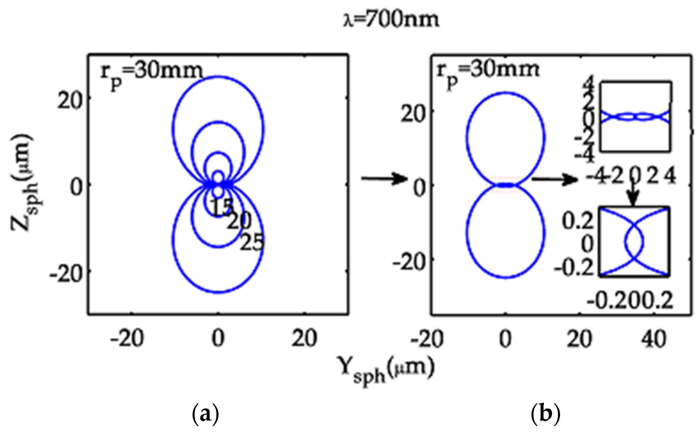
The spherical aberration curves of the model optical system for the center wavelength (Figure 2) are more complicated than common circular patterns of a centered lens system.

The spherical aberration curve is a circle of r_p³E₃₀₀₀ only when E₃₀₀₀ = E₁₂₀₀ = F₀₃₀₀ = F₂₁₀₀ is met. This condition is satisfied by an axially symmetric centered Offner optical system, which is the same as both a single mirror and a centered double-mirror system, yielding a concentric circular pattern for various values of r_p.

5.2.2. Coma

The coma of the concentric Offner optical system under consideration is expressed by:

$$\begin{array}{l}{Y}_{coma}=E_{2000}{\mathsf{\omega }}_1^2+E_{2010}{\mathsf{\omega }}_1^{2}z+E_{0210}{l}_1^{2}z+E_{1101}{\mathsf{\omega }}_1{l}_{1}s,\\ Z_{coma}=F_{1100}{\mathsf{\omega }}_1{l}_1+F_{2001}{\mathsf{\omega }}_1^{2}s+F_{1110}{\mathsf{\omega }}_1{l}_{1}z+F_{0201}{l}_1^{2}s\end{array}$$

(40)

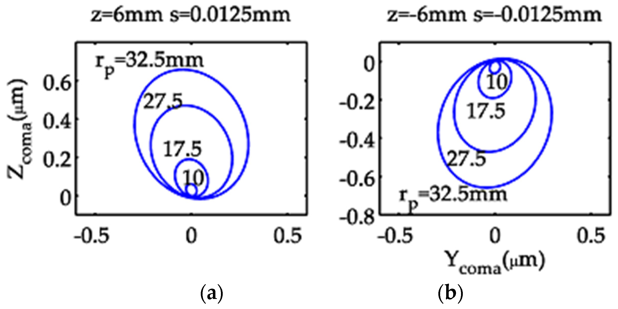
Substitution of Equation (37) into Equation (40) yields:

$$\begin{array}{l}a{\left\{\frac{2Y_{coma}}{r^2}-\left[E_{2000}+s(E_{2001}+E_{0201})\right]\right\}}^2+b{\left\{\frac{2Z_{coma}}{r^2}-z(F_{2010}+F_{0210})\right\}}^2\\ -2h\left\{\frac{2Y_{coma}}{r^2}-\left[E_{2000}+s(E_{2001}+E_{0201})\right]\right\}\left\{\frac{2Z_{coma}}{r^2}-z(F_{2010}+F_{0210})\right\}=c^2,\end{array}$$

(41)

where

$$\begin{array}{l}a={(F_{1100}+s{F}_{1101})}^2+z^2{(F_{2010}-F_{0210})}^2,\\ b={\left[E_{2000}+s(E_{2001}-E_{0201})\right]}^2+z^2{E}_{1110}^2,\\ c=(F_{1100}+s{F}_{1101})\left[E_{2000}+s(E_{2001}-E_{0201})\right]-z^2{E}_{1110}(F_{2010}-F_{0210}),\\ h=z\left\{E_{1110}(F_{1100}+s{F}_{1101})+(F_{2010}-F_{0210})\left[E_{2000}+s(E_{2001}-E_{0201})\right]\right\}.\end{array}$$

(42)

With Equation (41) describing an ellipse, the model optical system produces elliptical patterns for different values of r_p (Figure 3).

5.2.3. Astigmatism

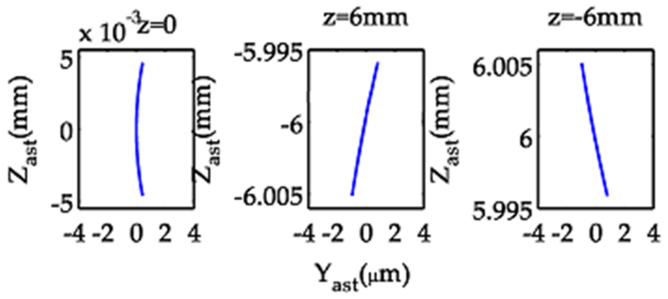
Astigmatism is an image defect caused by two mutually perpendicular line images, one at (r₂′)_M and the other at (r₂′)_S. Astigmatism of the concentric Offner optical system is represented by:

$$\begin{array}{l}{Y}_{ast}=E_{0001}s+E_{0200}{l}_1^2+E_{0110}{l}_{1}z+E_{0020}{z}^2,\\ Z_{ast}=F_{0100}{l}_1+F_{0010}z.\end{array}$$

(43)

which transforms to

$$Y_{ast}=E_{0200}{\left[\frac{Z_{ast}}{F_{0100}}+\left(\frac{E_{0110}}{2E_{0200}}-\frac{F_{0010}}{F_{0100}}\right)z\right]}^2+\left(E_{0020}-\frac{E_{0110}^2}{4E_{0200}}\right)z^2+E_{0001}s.$$

(44)

The astigmatic curves obtained from the model optical system appear as crescent-shaped patterns (Figure 4).

5.2.4. Distortion

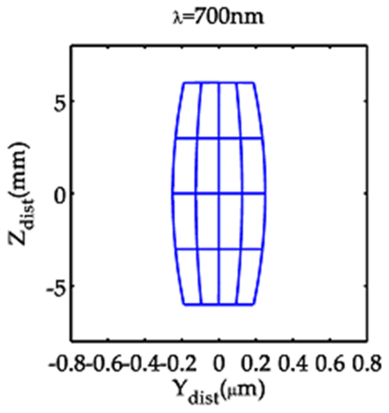
Distortion is the deviation between the actual image height and the ideal image height of the chief ray originating from a source point (0, s, z) and passing through the vertex O₁. In the ray-tracing formulas, the distortion is expressed as

$$\begin{array}{l}{Y}_{dist}=E_{0001}s+E_{0020}{z}^2+E_{0002}{s}^2+E_{0021}{z}^{2}s+E_{0003}{s}^3,\\ Z_{dist}=F_{0010}z+F_{0011}zs+F_{0030}{z}^3+F_{0012}z{s}^2.\end{array}$$

(45)

which manifests as a barrel-like structure from the model optical system (Figure 5). Because of the use of a very narrow slit illuminant, the distortions are visible in the Z direction and not in the Y direction.

6. Analysis of Diagram and Discussion

In Section 5, the evaluation of individual aberrations in the model optical system was presented using aberration curves, facilitating a better understanding of the imaging properties of the Offner system. More importantly, such an evaluation method helps to design and optimize the Offner system with an aberration-correction convex grating for different requirements.

However, before adopting the spot diagram formulas (25) and (26) in the design of an Offner system and its grating, the equations need to be critically evaluated in a comparison with exact ray-tracing. Here we compare spot diagrams computed from Equations (25) and (26) with those determined by the exact ray tracing using ZEMAX configured with a model Offner system equipped with a holographic convex grating.

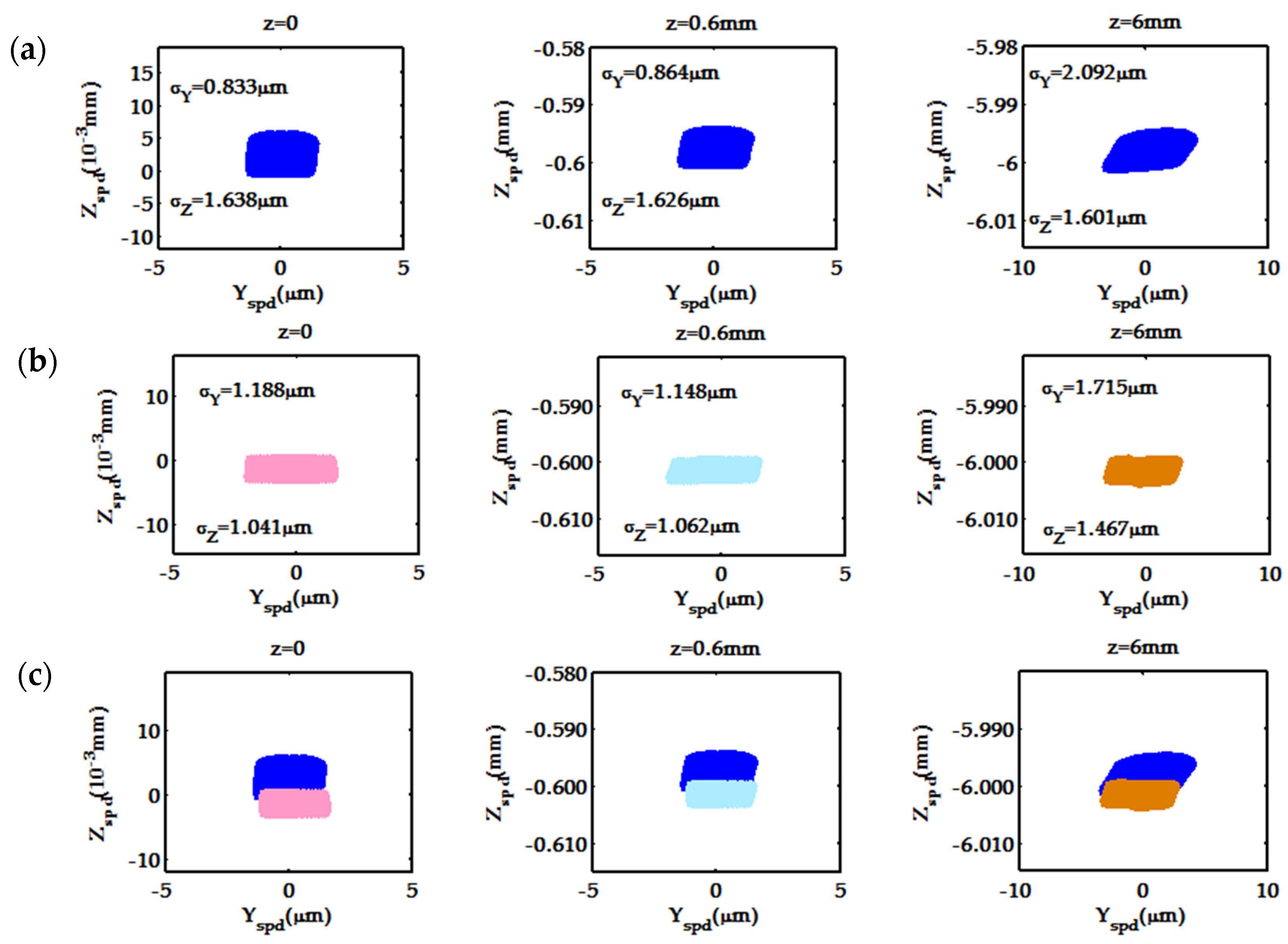
Because of the large z value and a relatively small s value in the model system, a portion of the spot diagram was constructed for various fields where we set z = 0, 0.6, and 6 mm with s = 0 without loss of generality. All the diagrams in Figure 6 and Figure 7 were constructed by generating 20000 rays of wavelength 700 nm covering the whole field of view. Spot diagrams in (a) and (b) were constructed for the selected point source presented in Figure 6, using the spot-diagram formulas and by ray tracing using ZEMAX, respectively. Clearly, the spot diagrams in (a) and (b) are similar in shape, but there are some deviations in size and position—especially in the Z direction; see Figure 6c.

The standard deviations σ_Y and σ_Z of the spots in the Y and Z directions (Figure 6a,b) illustrate the similarity in spot shape. The difference between the standard deviations of corresponding individual spots is smaller than 0.4 μm in the Y direction and 0.65 μm in the Z direction. Nearly the same dispersion tendency is seen depending on the system aberrations for the spot diagrams generated by both the present theoretical model and the simulation model of ZEMAX.

Figure 7a shows the deviations of individual spots obtained by the spot-diagram formulas from the corresponding ideal image points (0,0,0), (0,0,0.6) and (0,0,6). Figure 7b shows the deviations of individual spots generated by ray tracing using ZEMAX from the corresponding ideal image points. The deviations between ideal image points and spots from a simulation model (such as the theoretical simulation model or the ZEMAX simulation model) depend on both the system aberrations and model errors. The root-mean-squares RMS_ΔY and RMS_ΔZ of the deviations are given in the respective diagrams. Here, distinctions between the individual corresponding spots in Figure 7a,b—both in size and position—are mainly determined by different model errors. However, the difference between RMS_ΔY and RMS_ΔZ of the spots in Figure 7a,b is smaller than 0.4 μm in the Y direction and 0.7 μm in the Z direction. Therefore, the present theoretical model is similarly as useful as the ZEMAX model in designing and optimizing the Offner optical system. Certainly, supplemented by the fourth- and higher-order aberration terms into the spot diagram formulas (25) and (26), more exact theoretical model may be developed.

7. Conclusions

In this paper, a more practical method is adopted, comparing the theoretical simulation model with the simulation model provided by the commercial software ZEMAX, and offers great practicality.

A third-order aberration geometric theory was developed for tracing rays through the Offner imaging spectrometer comprising an extended source, two concave mirrors, a convex diffraction grating, and an image plane based on Fermat’s principle. The proposed theory provides analytic formulas for individual aberrations and spot diagrams. Following on from Namioka’s work, aberrations were analyzed and certain aberration curves were illustrated for a corresponding model optical system. The validity of the theoretical model was evaluated in a comparison with a simulation model provided by the commercial software ZEMAX and that of an actual model optical system. The results indicate the proposed theoretical model has great utility and practicality.

References

- Huang, H.; Li, X.T.; Cen, Z.F. Optical system design for a shortwave infrared imaging spectrometer. In Optical Design and Testing V; Society of Photo-Optical Instrumentation Engineers: Bellingham, WA, USA, 2012; Volume 85570R, pp. 1–10. [Google Scholar]
- Jacob, R.; Aaron, B.; Kevin, P.T.; Jannick, P.R. Freeform spectrometer enabling increased compactness. Light Sci. Appl. 2017, 6, 10. [Google Scholar]
- Liu, C.; Christoph, S.; Thomas, F.P.; Uwe, D.Z.; Herbert, G. Optical Design and Tolerancing of a Hyperspectral Imaging Spectrometer; Society of Photo-Optical Instrumentation Engineers: Bellingham, WA, USA, 2016; Volume 9947, pp. 1–10. [Google Scholar]
- Pang, Y.J.; Zhang, Y.X.; Yang, H.D.; Liu, Z.Y.; Huang, Z.H.; Jin, G.F. Compact high-resolution spectrometer using two plane gratings with triple dispersion. Opt. Express 2018, 26, 6382–6391. [Google Scholar] [CrossRef] [PubMed]
- Prieto-Blanco, X.; Montero-Orille, C.; Couce, B.; de la Fuente, R. Analytical design of an Offner imaging spectrometer. Opt. Express 2006, 20, 9156–9168. [Google Scholar] [CrossRef] [PubMed]
- Tang, T.J.; Zhang, Z.; Wang, B.H. Design of visible/infrared double-band spectral imager. J. Phys. Conf. Ser. 2016, 680, 1–6. [Google Scholar]
- Zhang, D.; Zheng, Y.Z. Hyperspectral Imaging System for UAV; Society of Photo-Optical Instrumentation Engineers: Bellingham, WA, USA, 2015; Volume 96780R, pp. 1–6. [Google Scholar]
- Kwo, D.; Lawrence, G.; Chrisp, M. Design of a Grating Spectrometer from a 1:1 Offner Mirror System; Society of Photo-Optical Instrumentation Engineers: Bellingham, WA, USA, 1987; Volume 818, pp. 275–279. [Google Scholar]
- Mouroulis, P. Low-distortion imaging spectrometer designs utilizing convex gratings. In Proceedings of the International Optical Design Conference, International Optical Design Conference, Kona, HI, USA, 8–12 June 1998; Volume 3482, pp. 594–601. [Google Scholar]
- Huang, Y.S.; Pei, Z.R.; Hong, R.J.; Li, B.C.; Zhang, D.W.; Xu, B.L.; Ni, Z.J.; Zhuang, S.L. Non-approximate method for designing Offner spectrometers. Optik 2014, 125, 4578–4582. [Google Scholar] [CrossRef]
- Seo, H.K.; Hong, J.K.; Soo, C. Aberration analysis of a concentric imaging spectrometer with a convex grating. Opt. Commun. 2014, 330, 6–10. [Google Scholar]
- Chrisp, M.P. Convex Diffraction Grating Imaging Spectrometer. Available online: http://www.freep-atentsonline.com/5880834.html (accessed on 12 October 2018).
- Xiang, L.Q.; Mikes, T. Corrected Concentric Spectrometer. Available online: http://www.freepate-ntsonline.com/6266140.html (accessed on 18 April 2018).
- Robert, L.L. Out-of-plane dispersion in an Offner spectrometer. Opt. Eng. 2007, 073004, 4. [Google Scholar]
- Prieto-Blanco, X.; Montero-Orille, C.; González-Núñez, H.; Mouriz, M.D.; Lago, E.L.; de la Fuente, R. Imaging with classical spherical diffraction gratings: The quadrature configuration. Opt. Soc. Am. A 2009, 11, 2400–2409. [Google Scholar] [CrossRef] [PubMed]
- Prieto-Blanco, X.; Montero-Orille, C.; González-Núñez, H.; Mouriz, M.D.; Lago, E.L.; de la Fuente, R. The Offner imaging spectrometer in quadrature. Opt. Express 2010, 12, 12756–12769. [Google Scholar] [CrossRef] [PubMed]
- Prieto-Blanco, X.; González-Núñez, H.; de la Fuente, R. Off-plane anastigmatic imaging in Offner spectrometers. Opt. Soc. Am. A 2011, 11, 2332–2339. [Google Scholar] [CrossRef] [PubMed]
- Prieto-Blanco, X.; de la Fuente, R. Compact Offner–Wynne imaging spectrometers. Opt. Commun. 2014, 328, 143–150. [Google Scholar] [CrossRef]
- Zhao, M.H.; Li, W.H.; Bayanheshig; Lv, Q. Aberration correction technique of Offner imaging spectrometer. Opt. Precis. Eng. 2017, 25, 3001–3011. [Google Scholar] [CrossRef]
- Zhao, X.L.; Bayanheshig; Li, W.H.; Jiang, Y.X.; Yang, S. Integrated design to complement aberrations of spherical focusing mirrors and concave holographic gratings in spectrometers. Acta Opt. Sin. 2016, 36, 10. [Google Scholar]
- Noda, H.; Namioka, T.; Seya, M. Ray tracing through holographic gratings. Opt. Soc. Am. 1974, 64, 1037–1042. [Google Scholar] [CrossRef]
- Namioka, T. Analytical representation of spot diagrams and its application to the design of monochromators. Nucl. Instrum. Methods Phys. Res. Sect. A Accel. Spectrometers Detect. Assoc. Equip. 1992, 319, 219–227. [Google Scholar] [CrossRef]
- Namioka, T.; Koike, M.; Content, D. Geometric theory of the ellipsoidal grating. Appl. Opt. 1999, 33, 7261–7274. [Google Scholar] [CrossRef] [PubMed]
- Masui, S.; Namioka, T. Geometric aberration theory of double-element optical systems. Opt. Soc. Am. A 1999, 16, 2253–2268. [Google Scholar] [CrossRef]
- Namioka, T.; Koike, M.; Masui, S. Geometric theory for the design of multielement Optical system. Opt. Precis. Eng. 2001, 9, 458–466. [Google Scholar]
- Namioka, T. Aspheric wave-front recording optics for holographic gratings. Appl. Opt. 1995, 34, 2180–2186. [Google Scholar] [CrossRef] [PubMed]
Figure 1.
Schematic diagram of an Offner configuration and its coordinate systems.
Figure 2.
Spherical aberration curves for λ = 700 nm of the model optical system in the meridional focal plane: (a) with rp = 30, 25, 20, 15 mm and (b) with rp = 30 mm (each inset is an enlargement of a central portion of the curve).
Figure 3.
Coma curves of the model optical system in the meridional focal plane, illustrating changes in pattern with rp, for settings (a) z = 6 mm and s = 0.0125 mm and (b) z = −6 mm and s = −0.0125 mm.
Figure 4.
Astigmatic curves of the model optical system in the meridional focal plane.
Figure 5.
Distortion patterns of the model optical system for a mesh-like source of dimension 25 μm (s) × 12 mm (z) with line separations of Δs = 6.25 μm and Δz = 3 mm.
Figure 6.
Spot diagrams constructed for the model optical system at λ = 700 nm with s = 0 from: (a) formulas (25) and (26); (b) ray tracing using ZEMAX; and (c) contrasted by overlaying (a) with (b).
Figure 7.
ΔY - ΔZ plots constructed for the model optical system at λ = 700 nm. (a) deviations, ΔY - ΔZ, of individual spots in Figure 6a from the corresponding ideal image points (0,0,0), (0,0,0.6) and (0,0,6); (b) deviations, ΔY - ΔZ, of individual spots in Figure 6b from the corresponding ideal image points (0,0,0), (0,0,0.6) and (0,0,6)7. Conclusions.