
Mechatronic Development and Vision Feedback Control of a Nanorobotics Manipulation System inside SEM for Nanodevice Assembly

 ,
,
Abstract
:1. Introduction
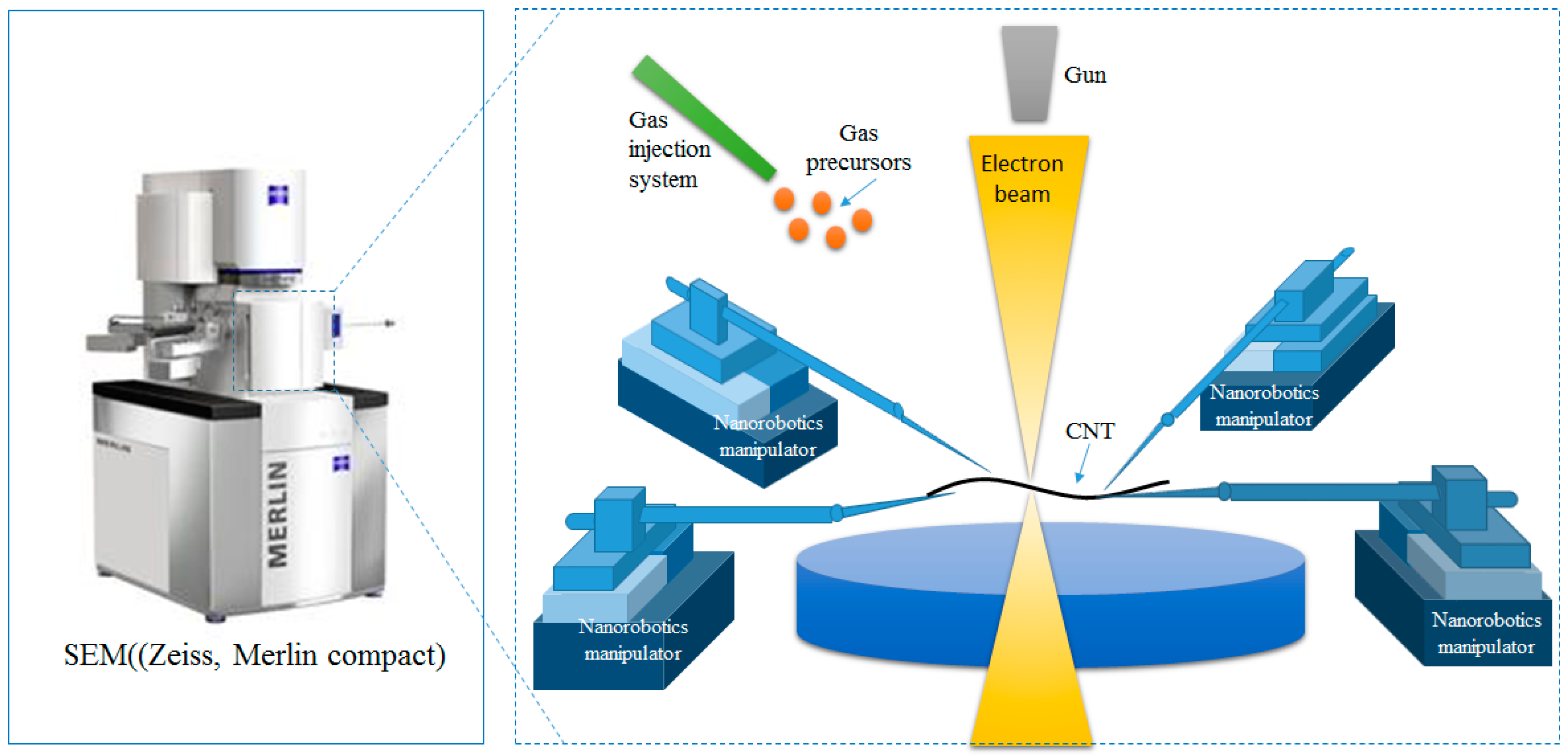
2. System Setup
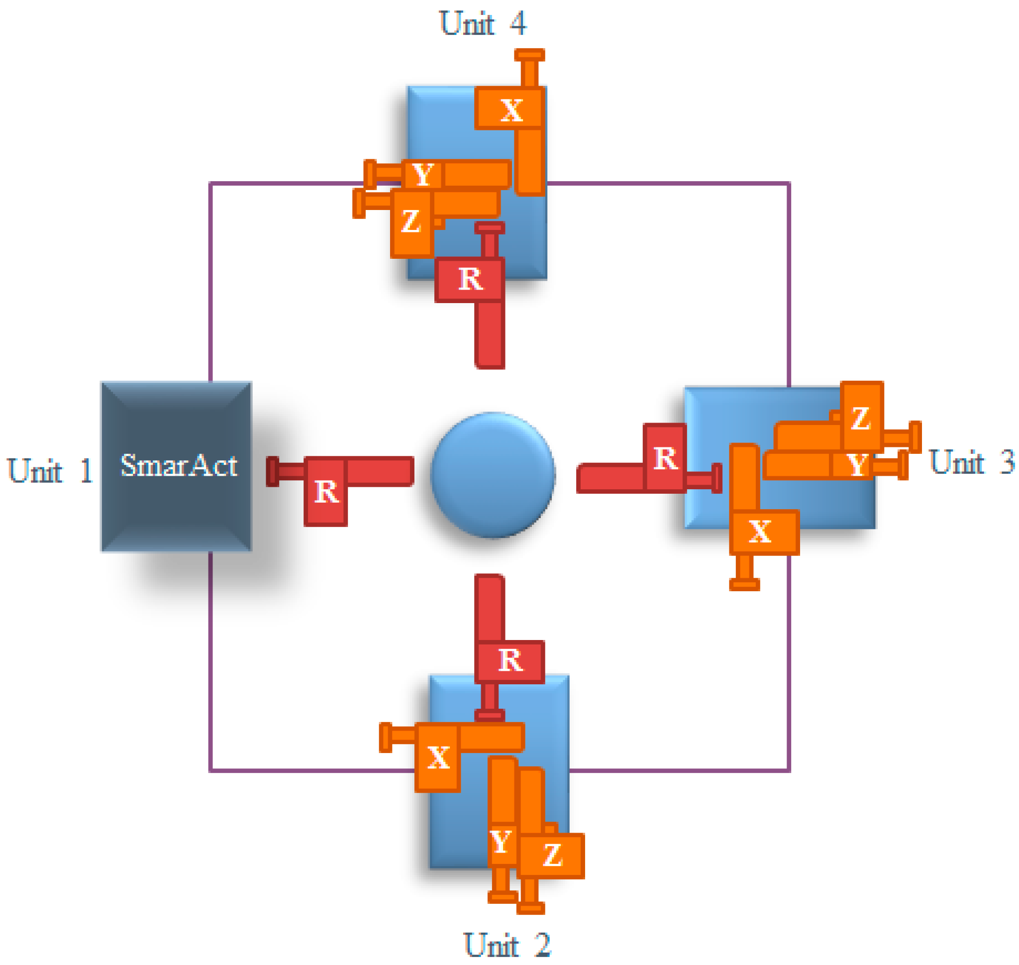
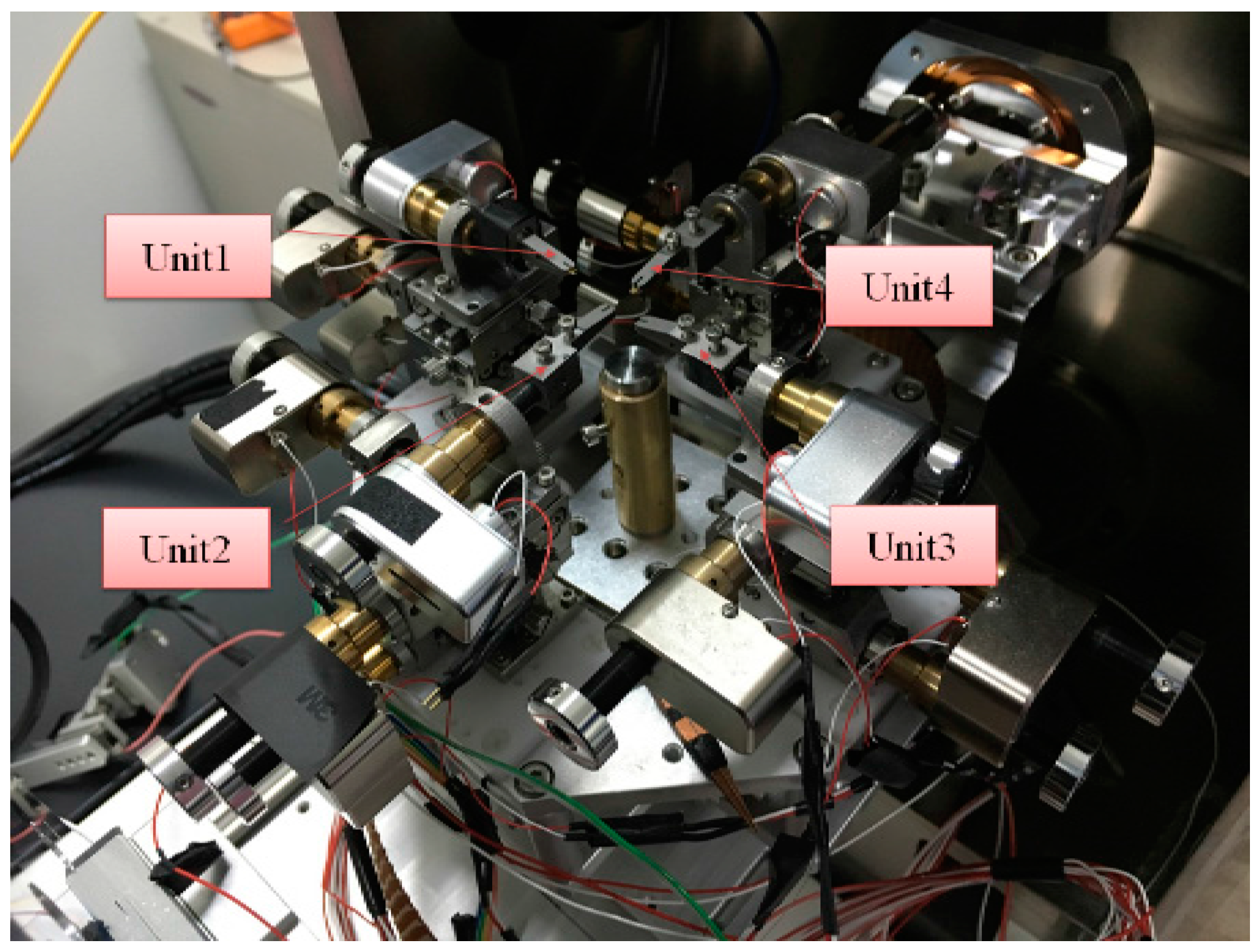
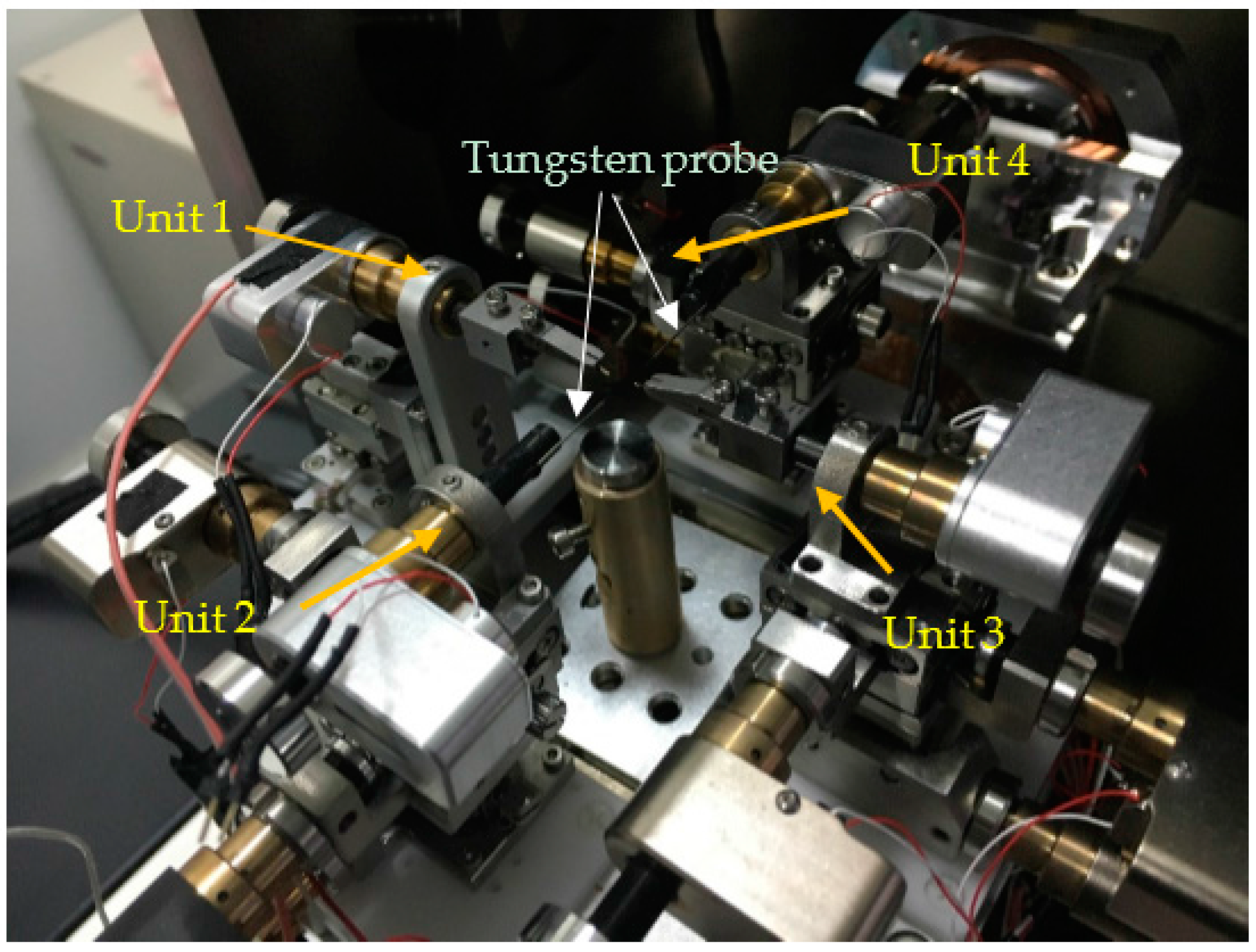
2.1. Mechanical Design and Developments of Nanorobotics Manipulation System
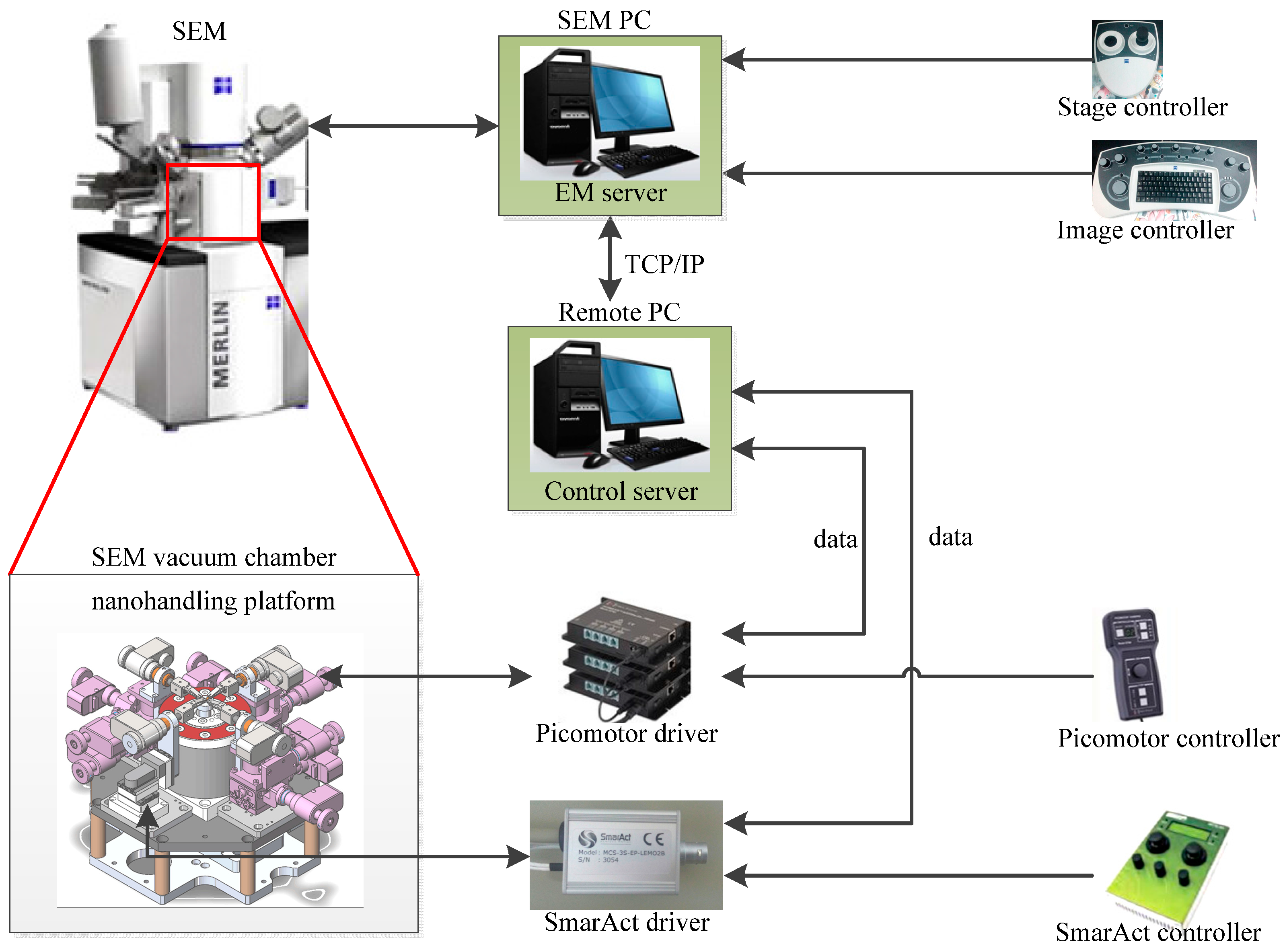
2.2. Electrical Connections and Driving
3. Theoretical Model
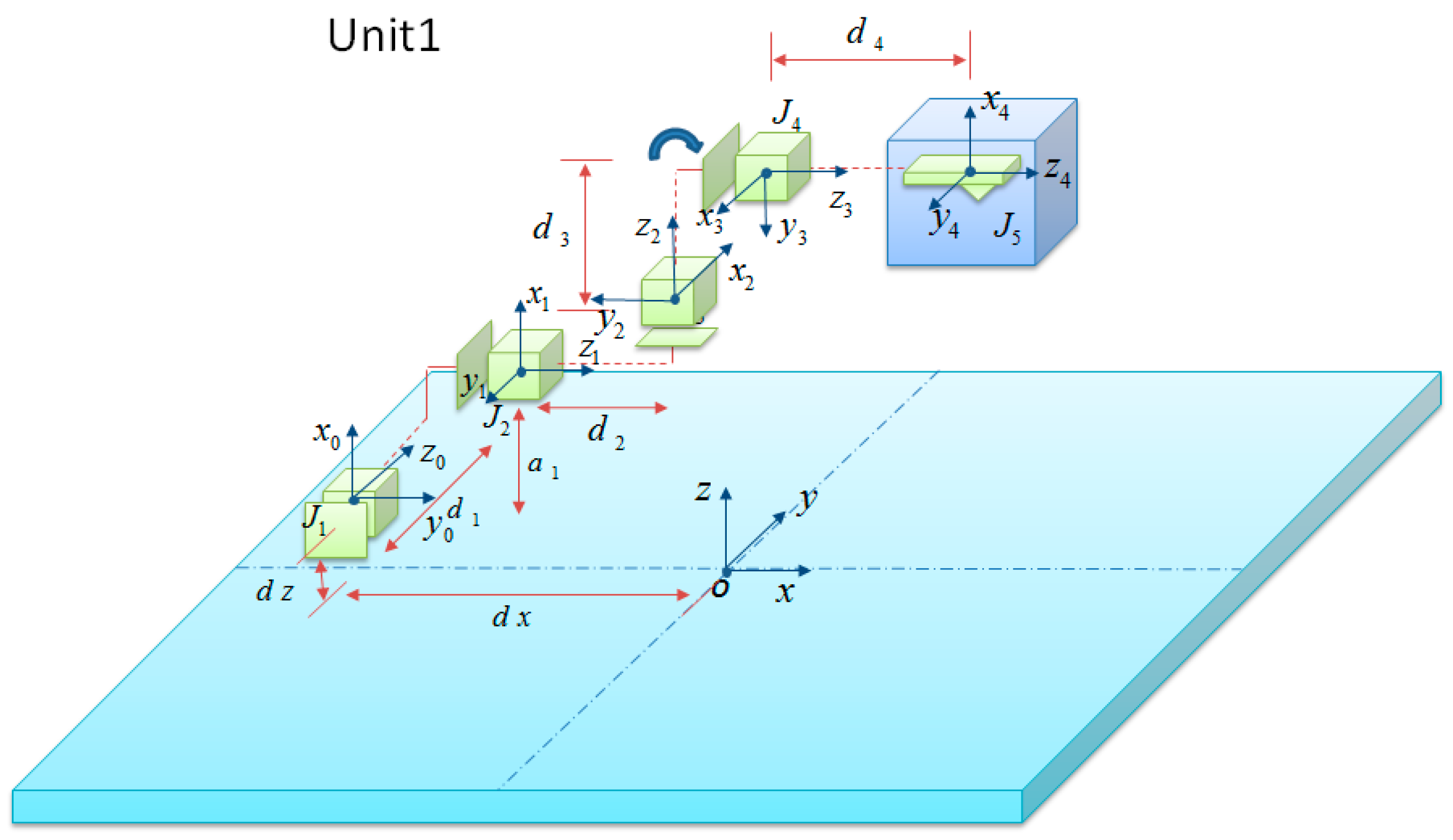
3.1. Theoretical Model of the Nanorobotics Manipulator
3.2. Theoretial Calculation Result of the Working Space
4. Manipulation Strategy and Vision Feedback Control
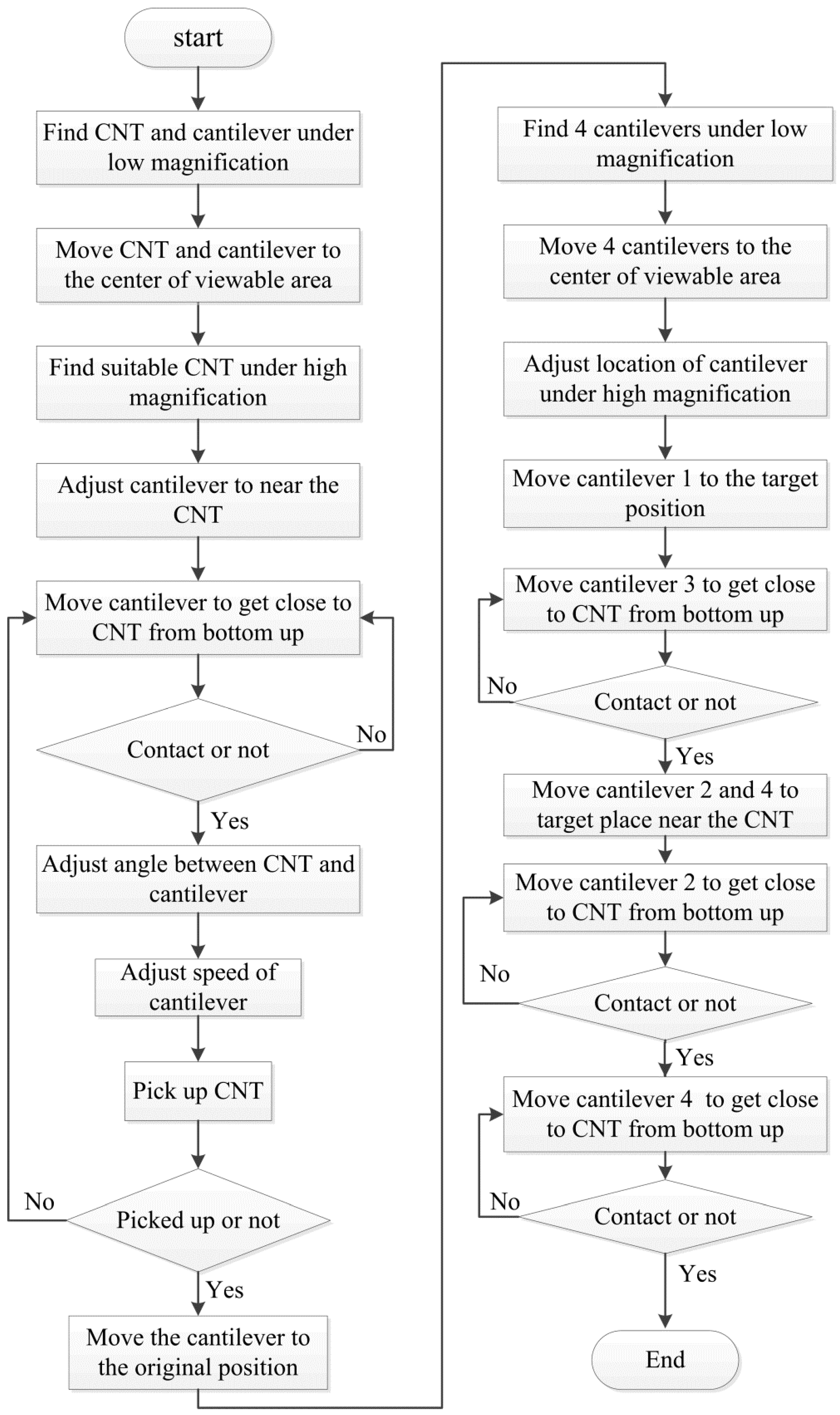
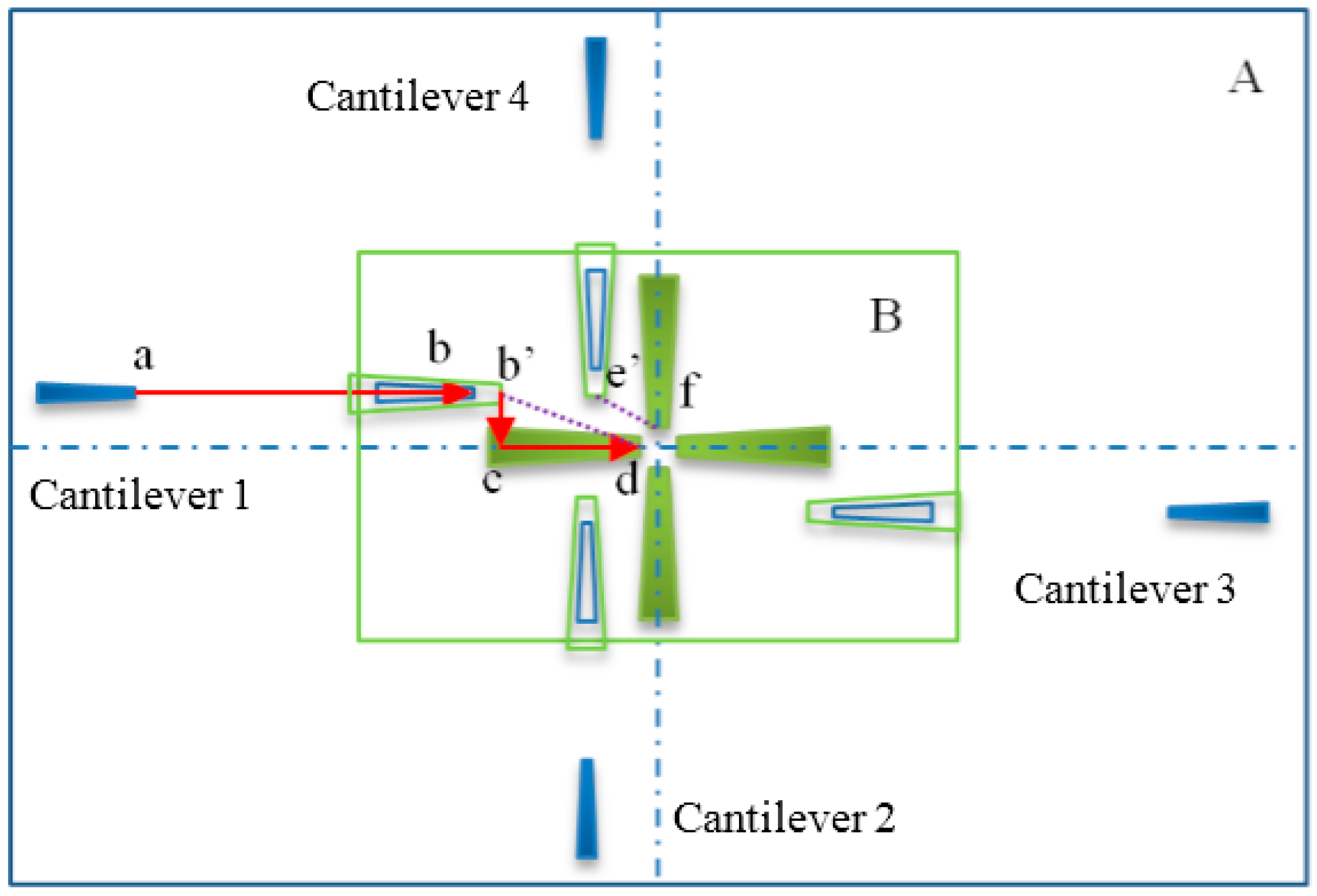
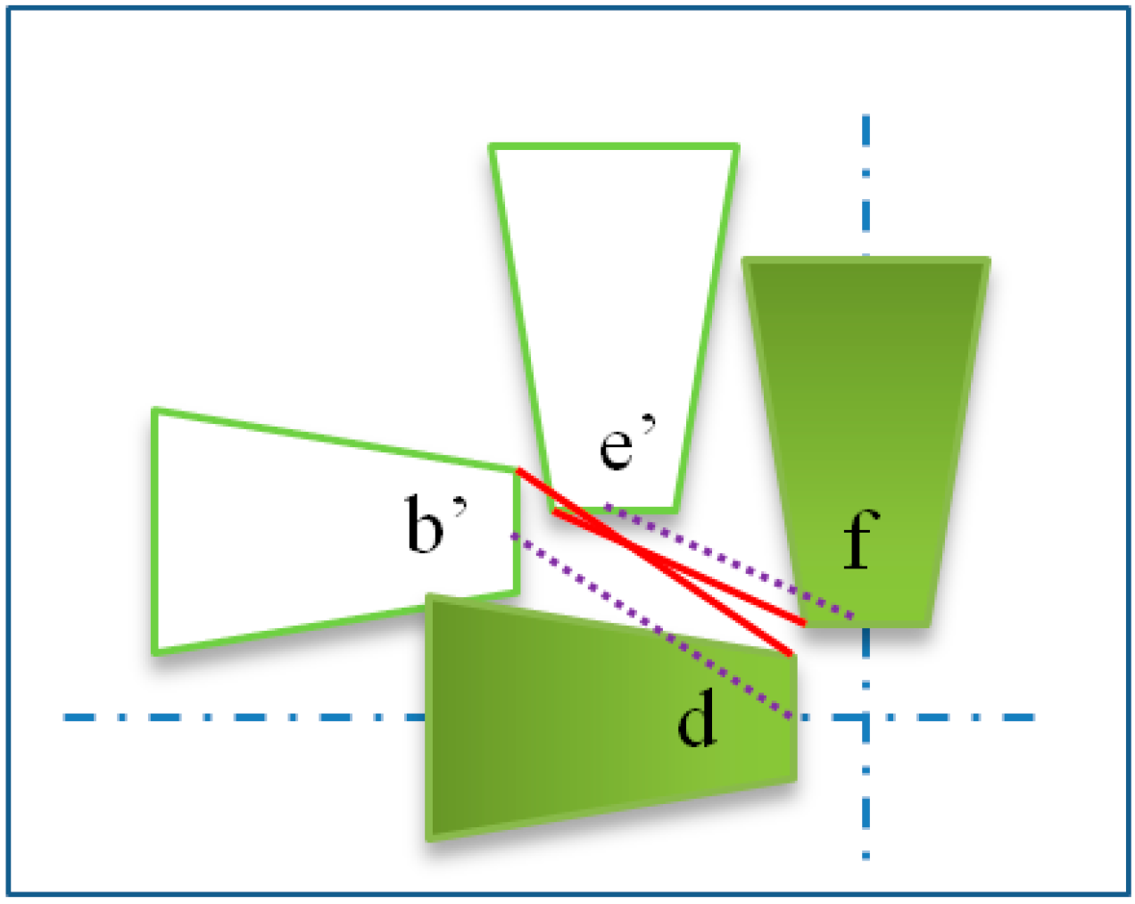
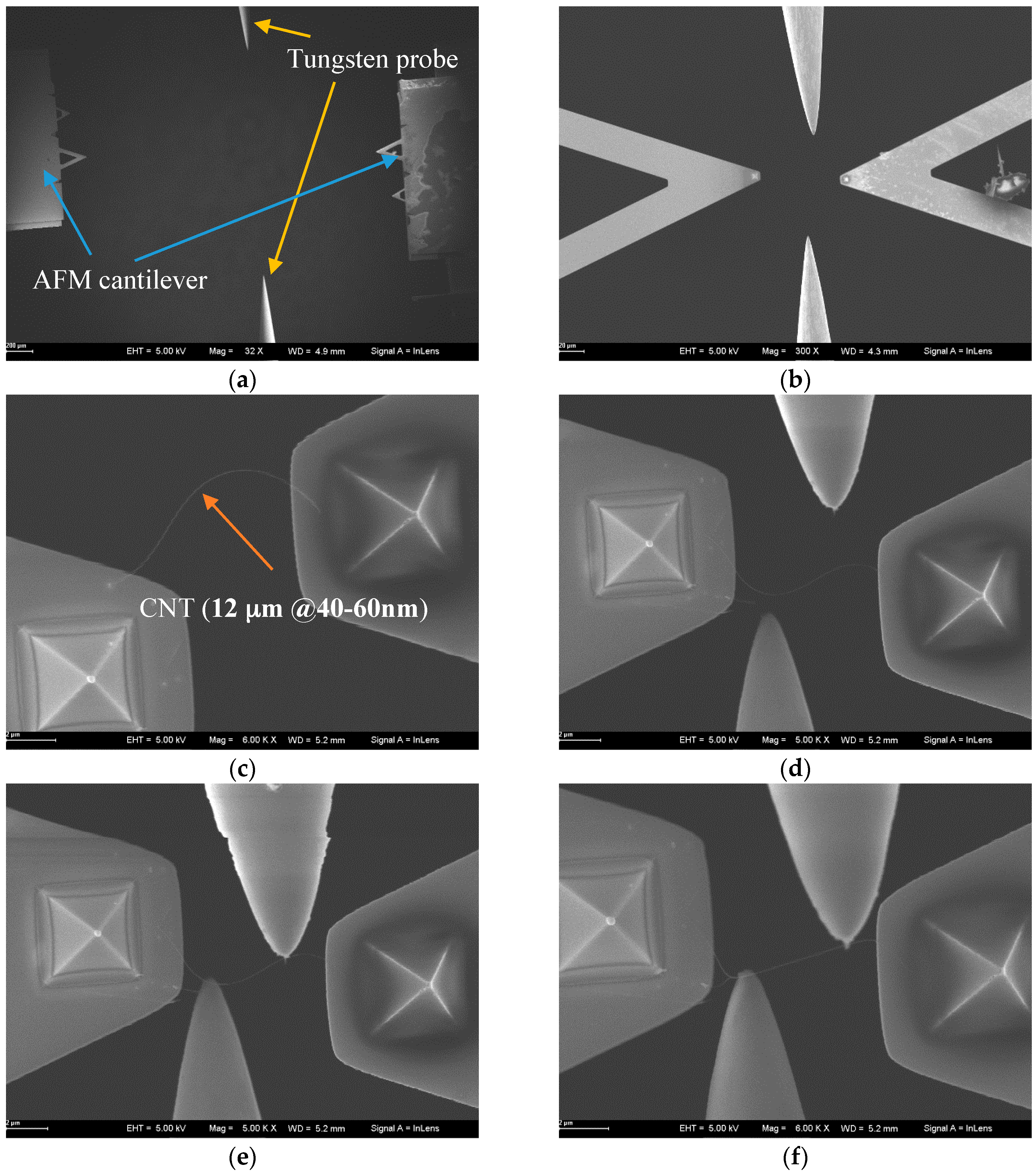
4.1. Manipulation Strategy for CNT Handling
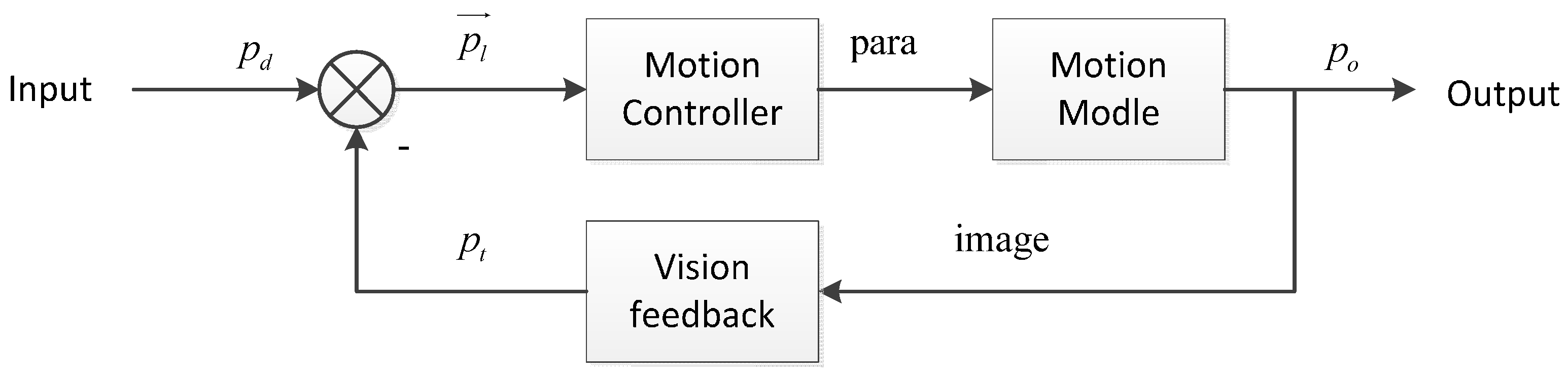
4.2. Visual Feedback Control inside the SEM
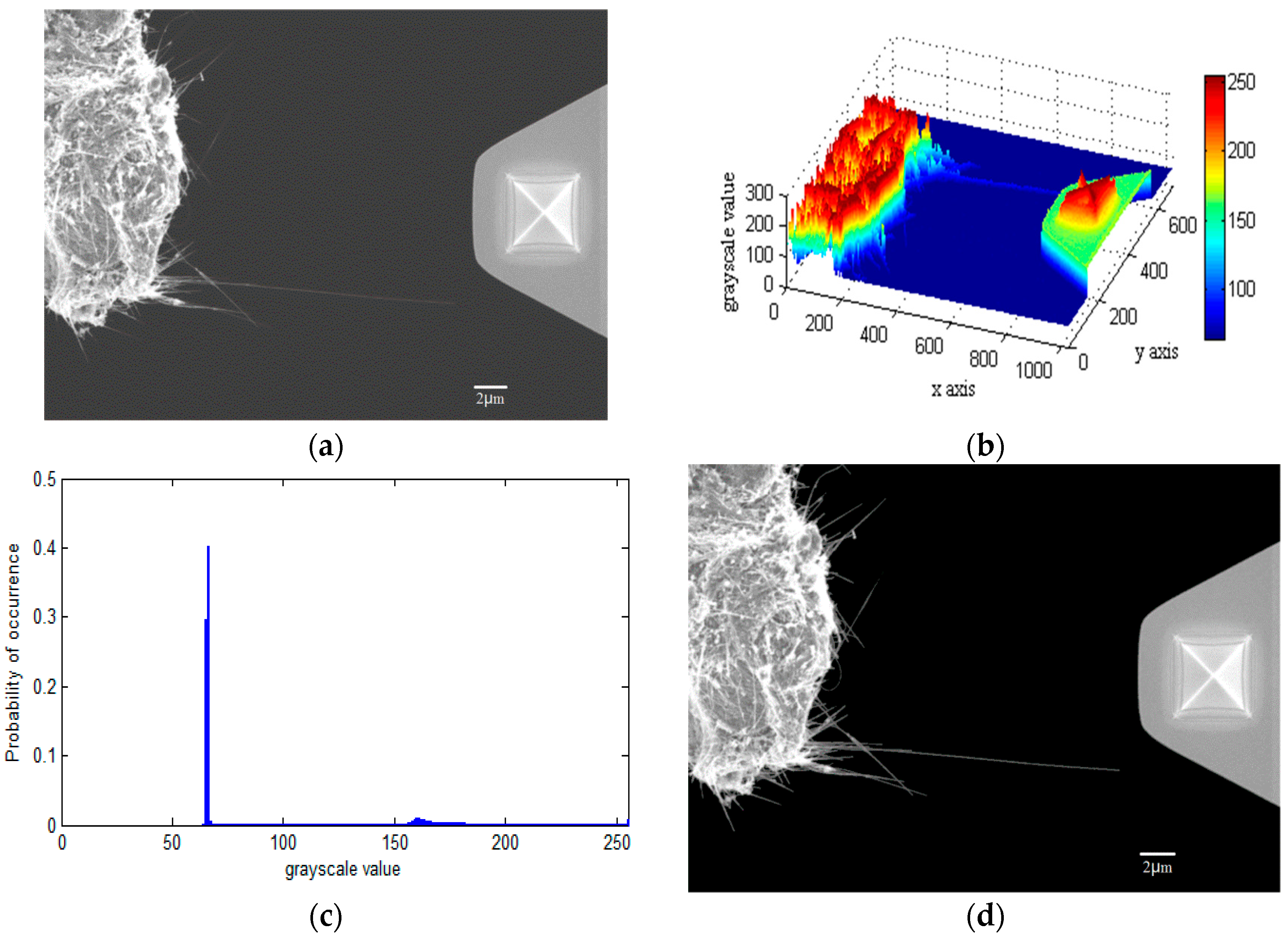
4.2.1. Automatic Binarization Method for Processing Scanned Images
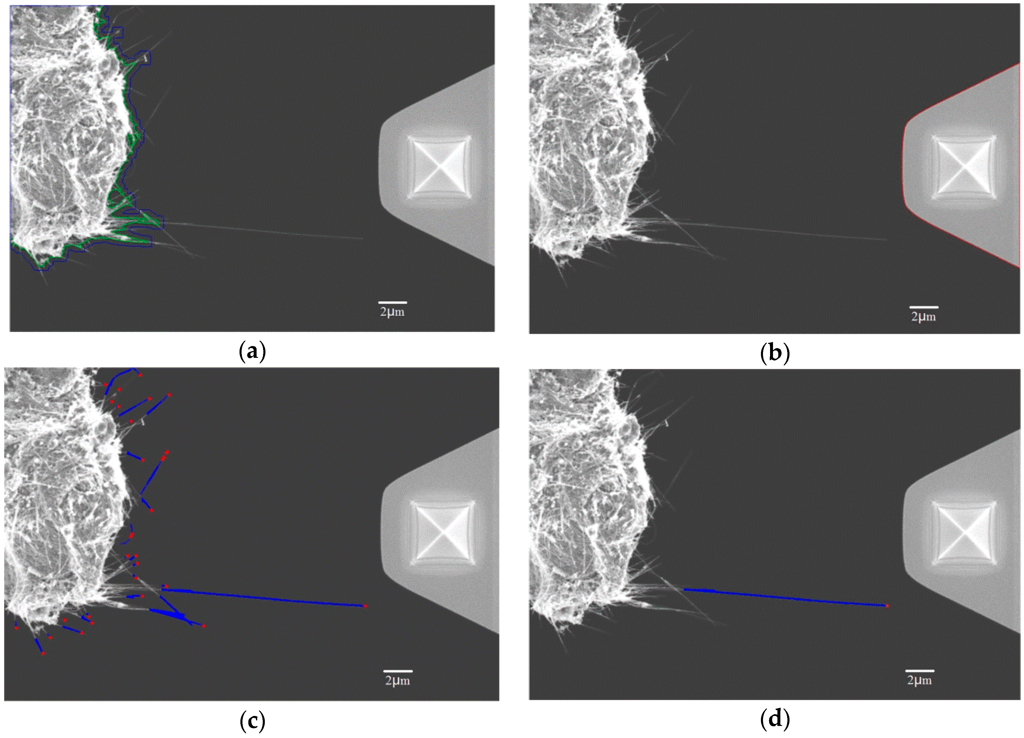
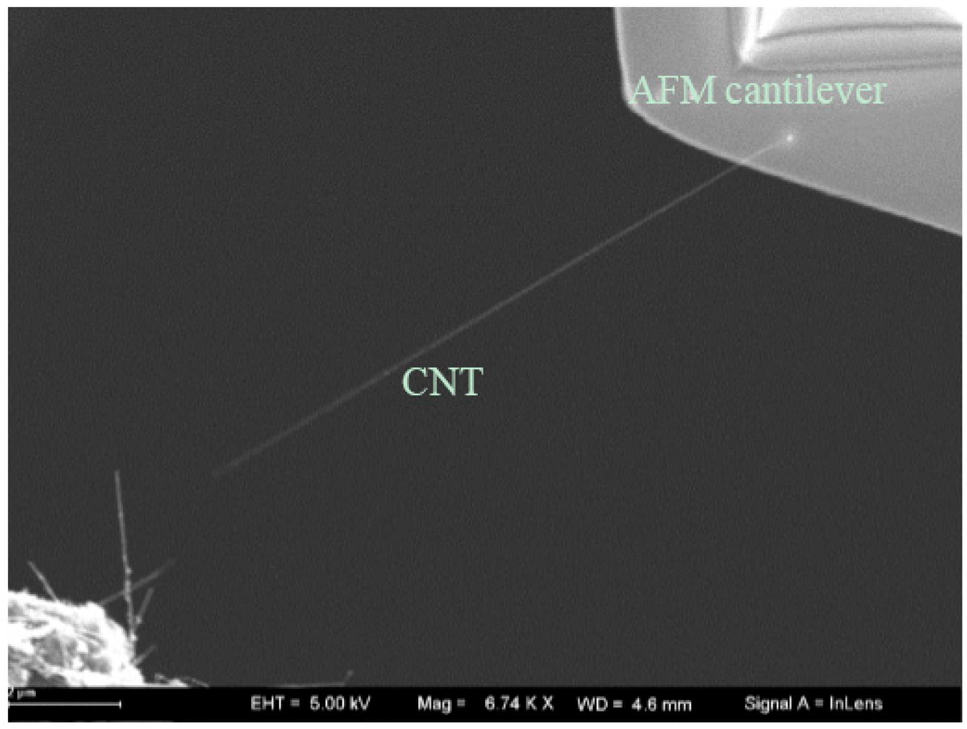
4.2.2. The Recognition of CNT and AFM Cantilever
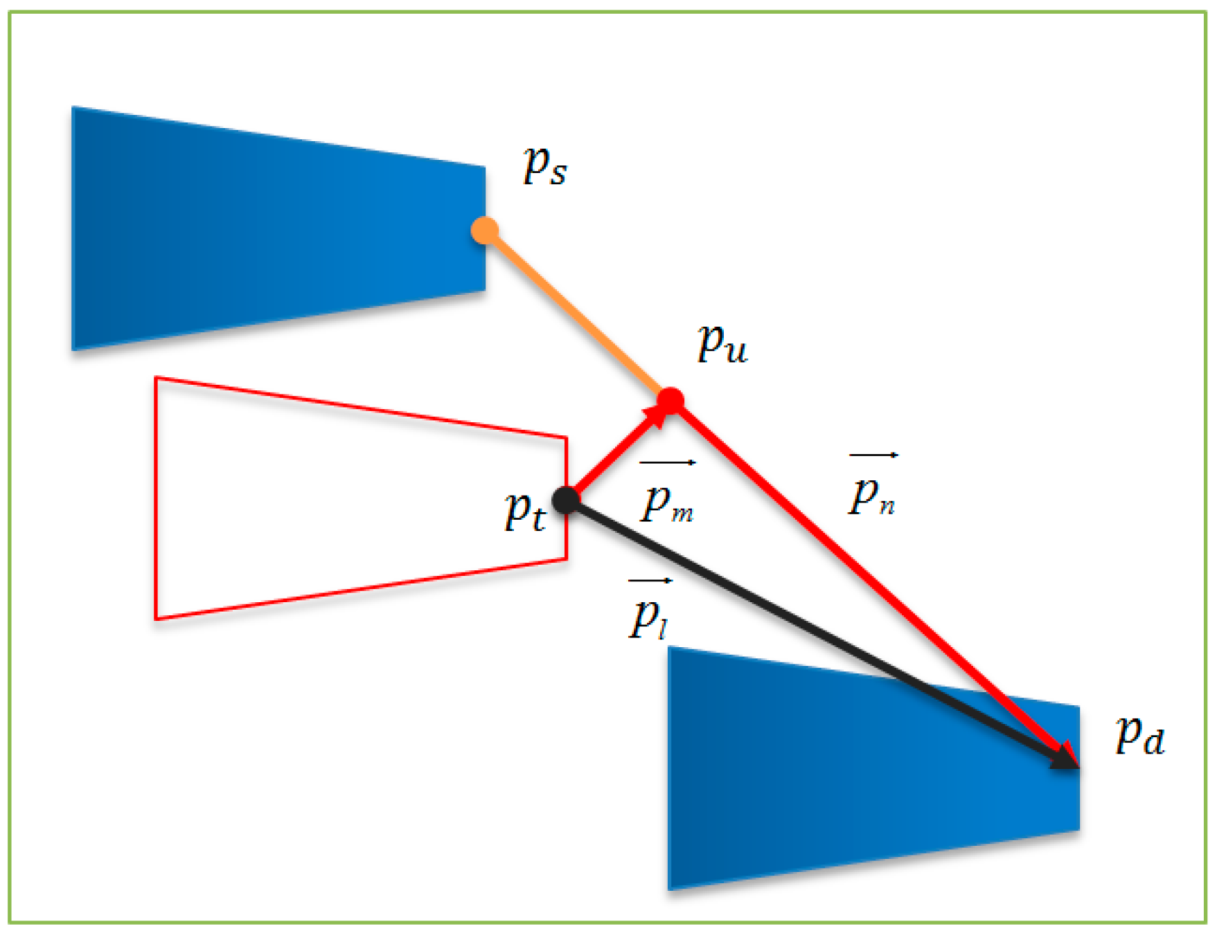
4.2.3. Closed-Loop Control of Microrobot-Based Vision Feedback
5. Experimental Implementation
6. Conclusions and Outlook
Acknowledgments
Author Contributions
Conflicts of Interest
References
- Iijima, S. Helical microtubules of graphitic carbon. Nature 1991, 354, 56–58. [Google Scholar] [CrossRef]
- Fukuda, T.; Arai, F.; Dong, L. Assembly of Nanodevices with Carbon Nanotubes through Nanorobotic Manipulation. In Proceedings of the IEEE, Altanta, GA, USA, 4–7 November 2003.
- Wei, H.; Li, Z.; Xiong, D.B.; Tian, Z.; Fan, G.; Qin, Z.; Zhang, D. Towards strong and stiff carbon nanotube-reinforced high-strength aluminum alloy composites through a microlaminated architecture design. Scr. Mater. 2014, 75, 30–33. [Google Scholar] [CrossRef]
- Tsai, T.Y.; Lee, C.Y.; Tai, N.H.; Tuan, W.H. Transfer of patterned vertically aligned carbon nanotubes onto plastic substrates for flexible electronics and field emission devices. Appl. Phys. Lett. 2009, 95. [Google Scholar] [CrossRef]
- Tao, C.; Wang, S.; Yang, Z.; Feng, Q.; Sun, X.; Li, L.; Wang, Z.S.; Peng, H. Flexible, light-weight, ultrastrong, and semiconductive carbon nanotube fibers for a highly efficient solar cell. Angew. Chem. 2011, 50, 1815–1819. [Google Scholar]
- Ishikawa, M.; Yoshimura, M.; Ueda, K. Carbon nanotube as a probe for friction force microscopy. Phys. B Condens. Matter 2002, 323, 184–186. [Google Scholar] [CrossRef]
- Chopra, S.; Mcguire, K.; Gothard, N.; Rao, A.M. Selective gas detection using a carbon nanotube sensor. Appl. Phys. Lett. 2003, 83, 2280–2282. [Google Scholar] [CrossRef]
- Franklin, A.D.; Luisier, M.; Han, S.J.; Tulevski, G.S.; Luisier, M.; Breslin, C.M.; Gignac, L.; Lundstrom, M.S.; Haensch, W. Sub-10 nm carbon nanotube transistor. Nano Lett. 2011, 12, 758–762. [Google Scholar] [CrossRef] [PubMed]
- Dong, L.; Zhang, L.; Bell, D.J.; Grützmacher, D.; Nelson, B.J. Nanorobotics for creating NEMS from 3D helical nanostructures. J. Phys. Conf. Ser. 2007, 61, 257–261. [Google Scholar] [CrossRef]
- Huang, J.; Huo, W.; Xu, W.; Mohammed, S.; Amirat, Y. Control of Upper-Limb Power-Assist Exoskeleton Using a Human-Robot Interface Based on Motion Intention Recognition. IEEE Trans. Autom. Sci. Eng. 2015, 12, 1257–1270. [Google Scholar] [CrossRef]
- Huang, J.; Ri, S.; Liu, L.; Wang, Y.; Kim, J.; Pak, G. Nonlinear Disturbance Observer-Based Dynamic Surface Control of Mobile Wheeled Inverted Pendulum. IEEE Trans. Control Syst. Technol. 2015, 23, 2400–2407. [Google Scholar] [CrossRef]
- Guthold, M.; Falvo, M.R.; Matthews, W.G.; Paulson, S.; Washburn, S.; Erie, D.; Superfine, R.; Brooks, F.P.; Taylor, R.M. Controlled manipulation of molecular samples with the nanomanipulator. In Proceedings of the IEEE/ASME Transactions on Mechatronics, Atlanta, GA, USA, 19–23 September 1999.
- Shen, Y.; Wan, W.; Zhang, L.; Li, Y.; Lu, Y.; Ding, W. Multidirectional Image Sensing for Microscopy Based on a Rotatable Robot. Sensors 2015, 15, 31566–31580. [Google Scholar] [CrossRef] [PubMed]
- Shi, C.; Luu, D.K.; Yang, Q.; Liu, J.; Chen, J.; Ru, C.; Xie, S.; Luo, J.; Ge, J.; Sun, Y. Recent advances in nanorobotic manipulation inside scanning electron microscopes. Microsyst. Nanoeng. 2016, 2. [Google Scholar] [CrossRef]
- Dong, L.; Arai, F.; Fukuda, T. 3D nanorobotic manipulation of nano-order objects inside SEM. In Proceedings of the IEEE International Symposium on Micromechatronics and Human Science, Nagoya, Japan, 22–25 October 2000.
- Fukuda, T.; Arai, F.; Dong, L. Nanorobotic systems. Int. J. Adv. Robot. Syst. 2005, 2, 264–275. [Google Scholar] [CrossRef]
- Saeidpourazar, R.; Jalili, N. Towards fused vision and force robust feedback control of nanorobotic-based manipulation and grasping. Mechatronics 2008, 18, 566–577. [Google Scholar] [CrossRef]
- Saeidpourazar, R.; Jalili, N. Nano-robotic manipulation using a RRP nanomanipulator: Part B—Robust control of manipulator’s tip using fused visual servoing and force sensor feedbacks. Appl. Math. Comput. 2008, 206, 628–642. [Google Scholar] [CrossRef]
- Eichhorn, V.; Fatikow, S.; Wortmann, T.; Stolle, C.; Edeler, C.; Jasper, D.; Sardan, O.; Boggild, P.; Boetsch, G.; Canales, C.; et al. NanoLab: A nanorobotic system for automated pick-and-place handling and characterization of CNTs. In Proceedings of the IEEE International Conference on Robotics & Automation, Kobe, Japan, 12–17 May 2009.
- Shen, Y.; Nakajima, M.; Zhang, Z.; Fukuda, T. Dynamic Force Characterization Microscopy Based on Integrated Nanorobotic AFM and SEM System for Detachment Process Study. IEEE/ASME Trans. Mech. 2015, 20, 3009–3017. [Google Scholar] [CrossRef]
- Ru, C.; Zhang, Y.; Sun, Y.; Zhong, Y.; Sun, X.; Hoyle, D.; Cotton, I. Automated four-point probe measurement of nanowires inside a scanning electron microscope. In Proceedings of the IEEE Conference on Automation Science and Engineering, Toronto, ON, Canada, 21–24 August 2010.
- Zhou, C.; Gong, Z.; Chen, B.K.; Cao, Z.; Yu, J.; Ru, C.; Tan, M.; Xie, S.; Sun, Y. A closed-loop controlled nanomanipulation system for probing nanostructures inside scanning electron microscopes. IEEE Trans. Mech. 2016, 21, 1233–1241. [Google Scholar] [CrossRef]
- Xie, H.; Régnier, S. High-efficiency automated nanomanipulation with parallel imaging/manipulation force microscopy. IEEE Trans. Nanotechnol. 2012, 11, 21–33. [Google Scholar] [CrossRef]
- Shang, W.; Lu, H.; Wan, W.; Fukuda, T.; Shen, Y. Vision-based Nano Robotic System for High-throughput Non-embedded Cell Cutting. Sci. Rep. 2016, 6. [Google Scholar] [CrossRef] [PubMed]
- Kreupl, F.; Graham, A.P.; Duesberg, G.S.; Steinhoegl, W.; Liebau, M.; Unger, E.; Hoenlein, W. Carbon nanotubes in interconnect applications. Microelectron. Eng. 2002, 64, 399–408. [Google Scholar] [CrossRef]
- Hoenlein, W.; Kreupl, F.; Duesberg, G.S.; Graham, A.P.; Liebau, M.; Seidel, R.V.; Unger, E. Carbon nanotube applications in microelectronics. IEEE Trans. Comp. Packag. Technol. 2004, 27, 629–634. [Google Scholar] [CrossRef]
- Tulevski, G.S.; Franklin, A.D.; Frank, D.; Lobez, J.M.; Cao, Q.; Park, H.; Afzali, A.; Han, S.J.; Hannon, J.B.; Haensch, W. Toward High-performance digital logic technology with carbon nanotubes. ACS Nano 2014, 8, 8730–8745. [Google Scholar] [CrossRef] [PubMed]
- Wang, Y.; Yang, Z.; Chen, T.; Sun, L.; Fukuda, T. CNT Handling with van de Waals Force inside an SEM for FET application. In Proceedings of the IEEE Conference on Nano/Micro Engineering and Molecular Systems, Matsushima Bay, Sendai, Japan, 17–20 April 2016.


| Parameters | Unit 1 | Units 2–4 |
|---|---|---|
| Model | SLC-1720-s/8301-UHV | TSDS-255C/8301-UHV |
| Dimensions (mm) | 33 × 33 × 30.5/63.5 × 32.2 × 56.5 | 66 × 66 × 45/63.5 × 32.2 × 56.5 |
| Travel (mm) | X ± 6, Y ± 6, Z ± 6 | XY ± 3, Z ± 3 |
| Rotate | ±360º | ±360º |
| Linear Resolution | 1 nm | 30 nm |
| Rotate Resolution | <1 micro-rad | <1 micro-rad |
| 1 | −90 | 0 | 0 | |
| 2 | −90 | 0 | −90 | |
| 3 | −90 | 0 | 180 | |
| 4 | 0 | 0 | −90 |
| Image Size (Pixels) | Scanning Speed | N | Scanning Cycle |
|---|---|---|---|
| 512 × 384 | 4 | 1 | 221.78 ms |
| 1024 × 768 | 4 | 1 | 735.01 ms |
| 1024 × 768 | 9 | 1 | 20.4 s |
| 1024 × 768 | 4 | 10 | 7.1 s |
| 2048 × 1536 | 4 | 1 | 2.7 s |
© 2016 by the authors; licensee MDPI, Basel, Switzerland. This article is an open access article distributed under the terms and conditions of the Creative Commons Attribution (CC-BY) license (http://creativecommons.org/licenses/by/4.0/).
Share and Cite
Yang, Z.; Wang, Y.; Yang, B.; Li, G.; Chen, T.; Nakajima, M.; Sun, L.; Fukuda, T. Mechatronic Development and Vision Feedback Control of a Nanorobotics Manipulation System inside SEM for Nanodevice Assembly. Sensors 2016, 16, 1479. https://doi.org/10.3390/s16091479
Yang Z, Wang Y, Yang B, Li G, Chen T, Nakajima M, Sun L, Fukuda T. Mechatronic Development and Vision Feedback Control of a Nanorobotics Manipulation System inside SEM for Nanodevice Assembly. Sensors. 2016; 16(9):1479. https://doi.org/10.3390/s16091479
Chicago/Turabian StyleYang, Zhan, Yaqiong Wang, Bin Yang, Guanghui Li, Tao Chen, Masahiro Nakajima, Lining Sun, and Toshio Fukuda. 2016. "Mechatronic Development and Vision Feedback Control of a Nanorobotics Manipulation System inside SEM for Nanodevice Assembly" Sensors 16, no. 9: 1479. https://doi.org/10.3390/s16091479