
An Adaptive INS-Aided PLL Tracking Method for GNSS Receivers in Harsh Environments


Abstract
:1. Introduction
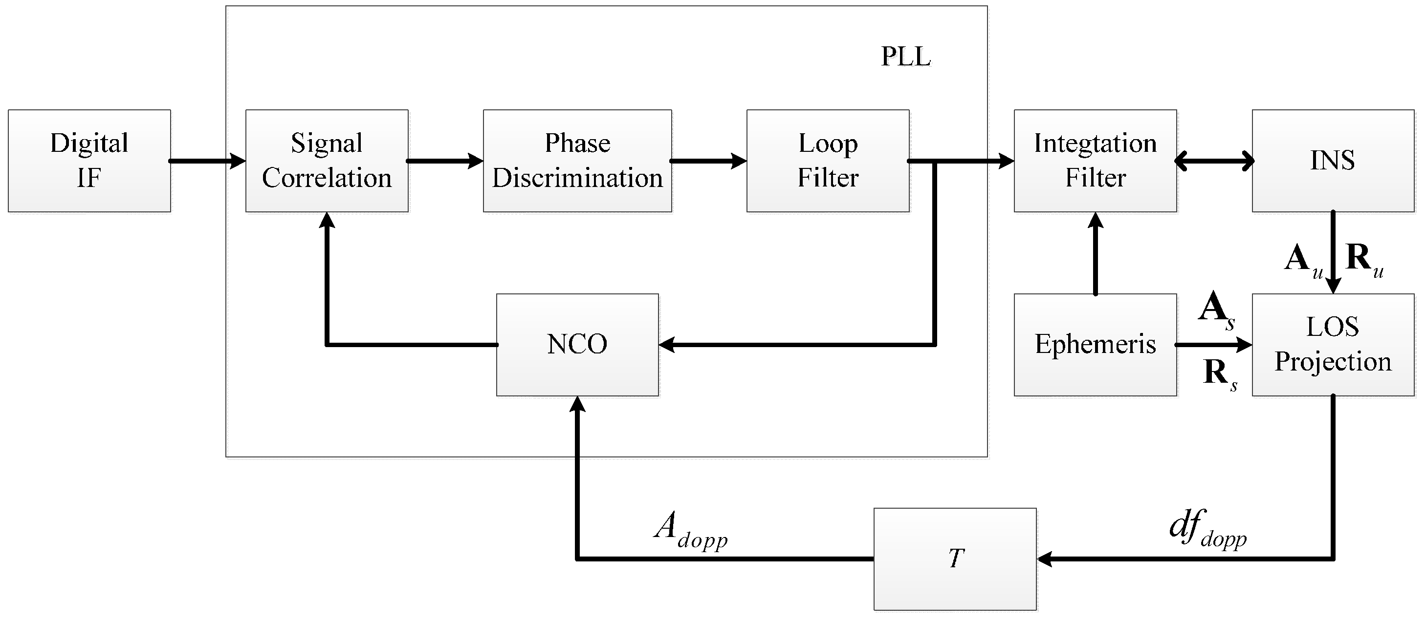
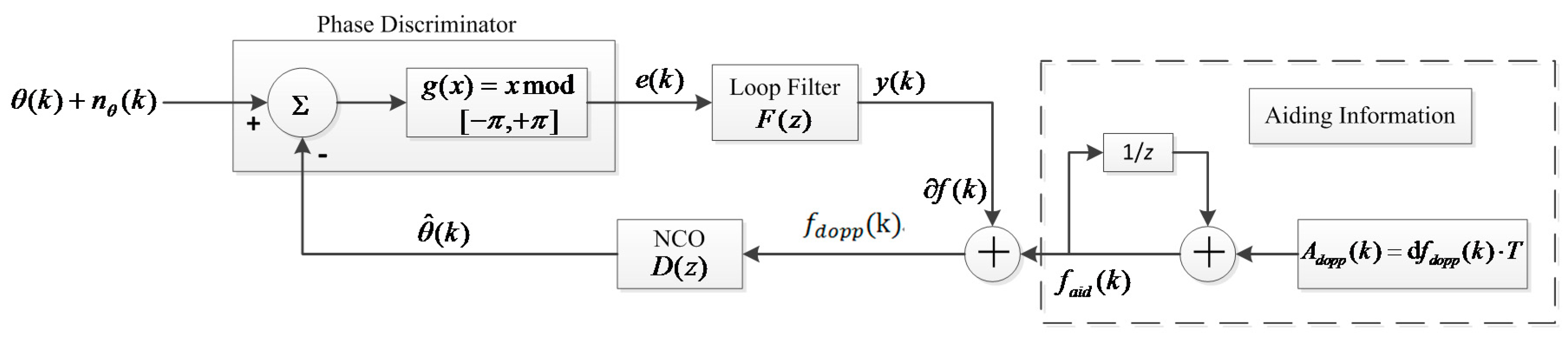
2. The Principle of Delta Doppler Aided PLL

3. Tracking Error Analysis of Delta Doppler Aided PLL
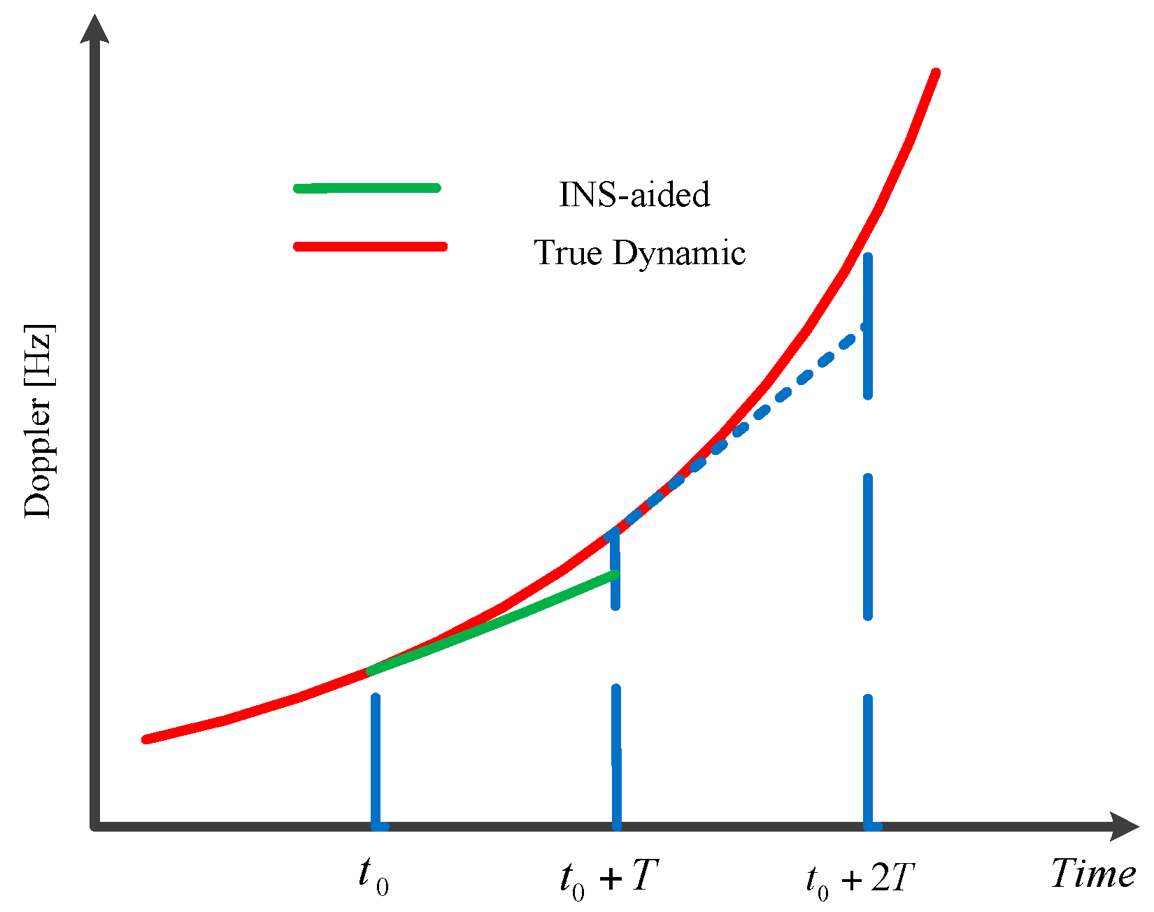
3.1. Dynamic Stress Error


3.2. Thermal Noise Error
3.3. Oscillator Phase Error
3.4. Stable Tracking Criterion of INS-Aided PLL
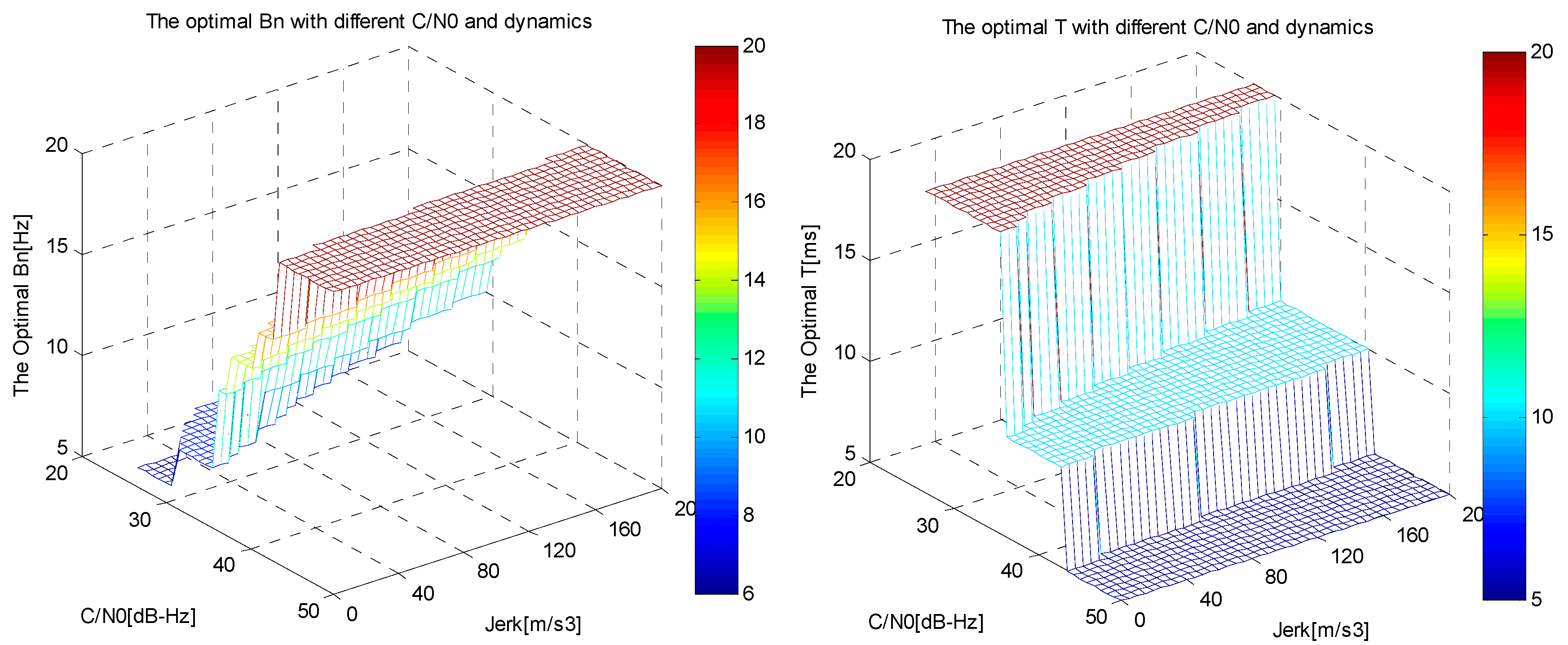
4. Adaptive Adjustments of Integration Time and Bandwidth of INS-Aided PLL
| Algorithm 1. The adaptive method for choosing the optimal noise bandwidth and integration time. |
Input:
|


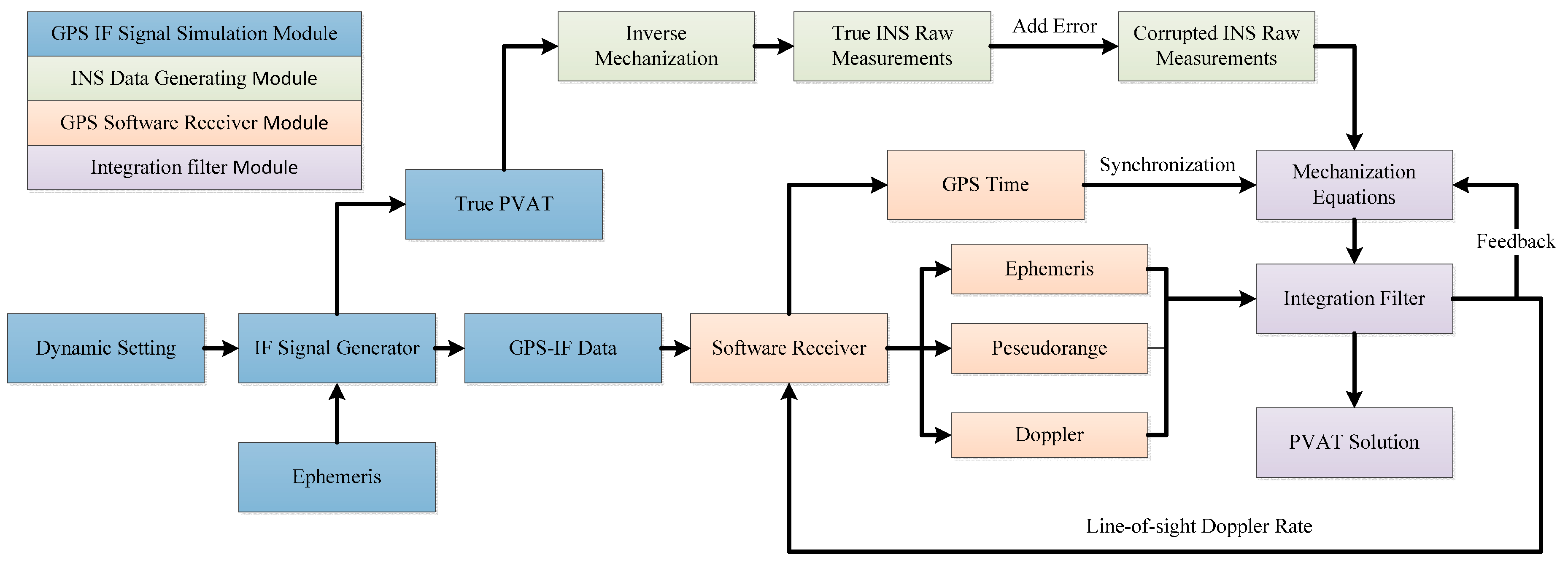
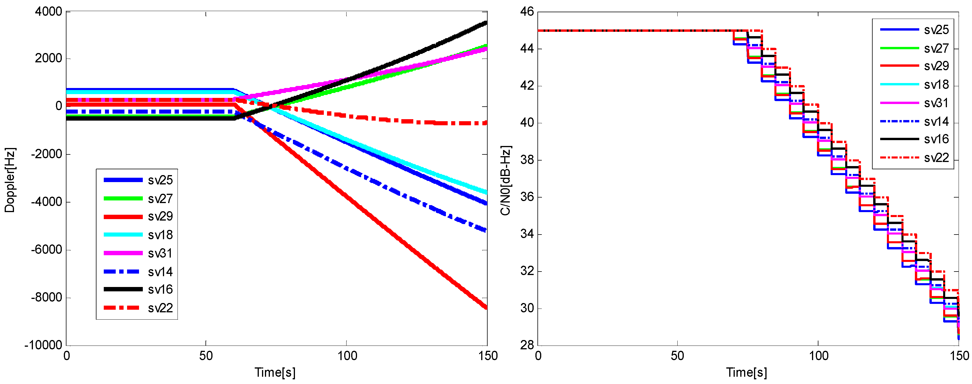
5. Software Simulation

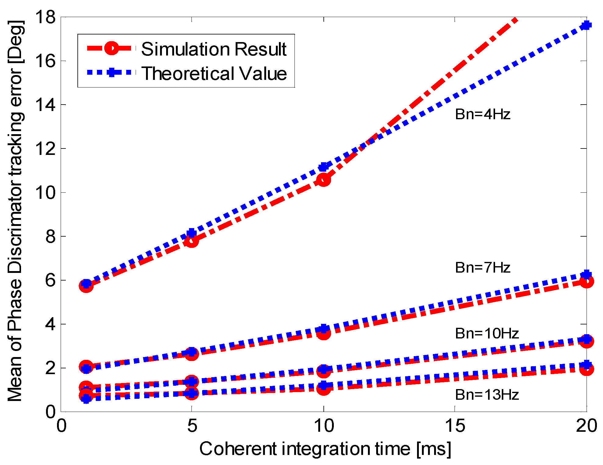
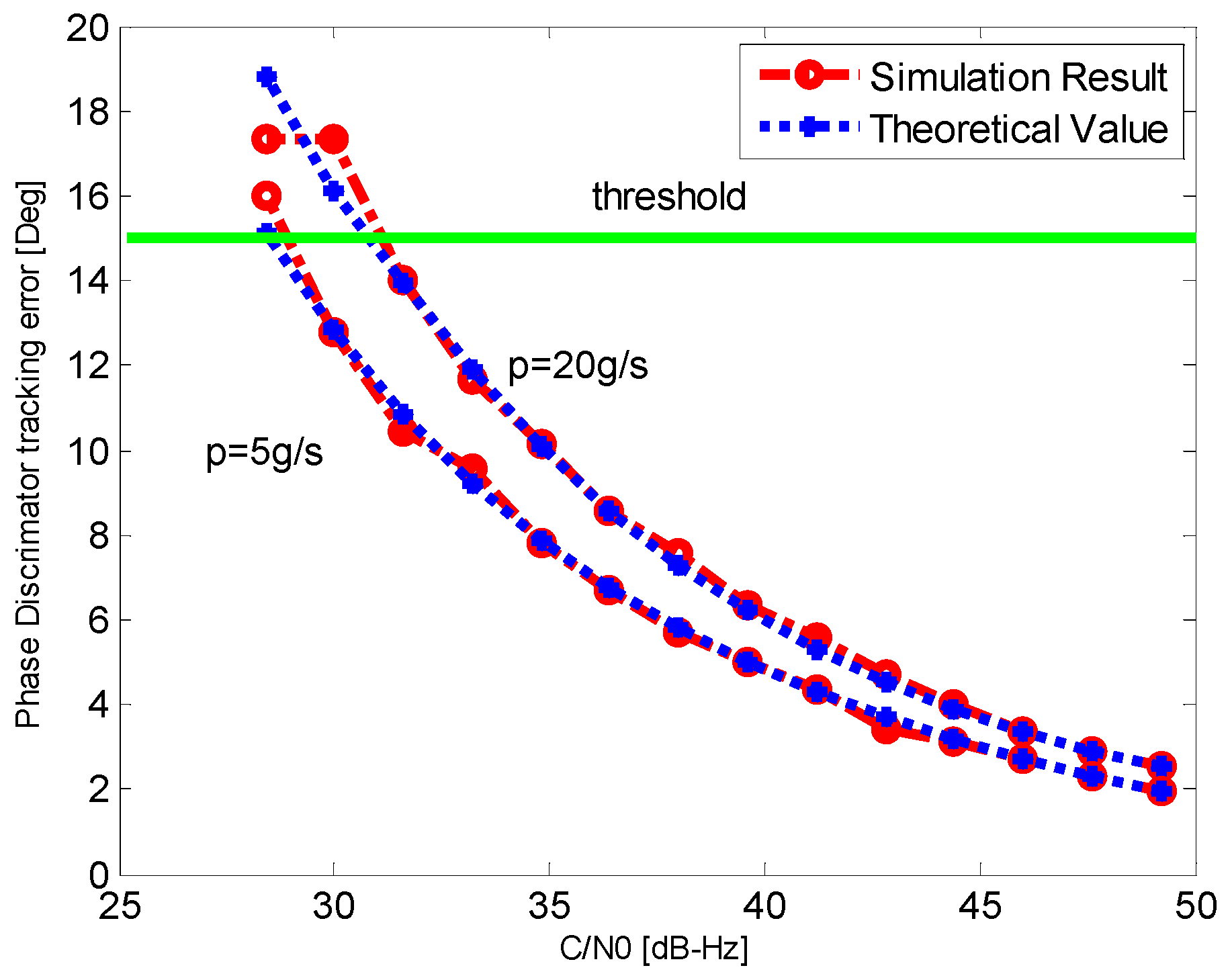
5.1. Validation of Dynamic Stress Error


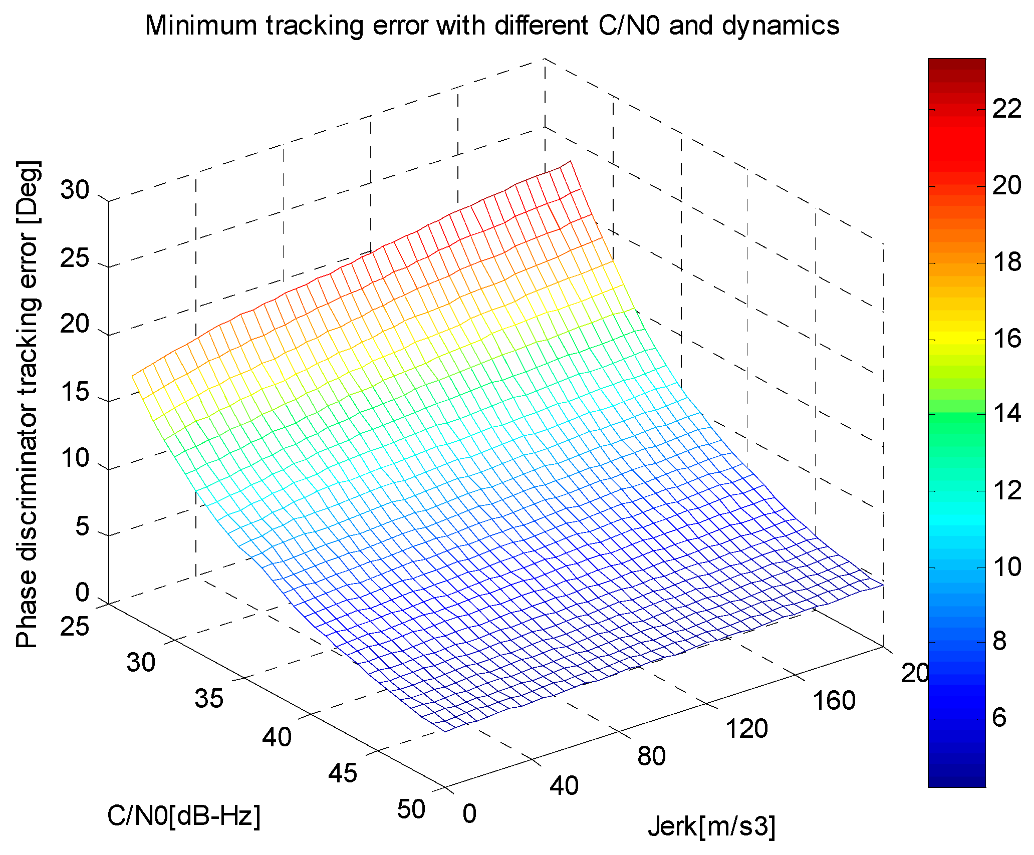
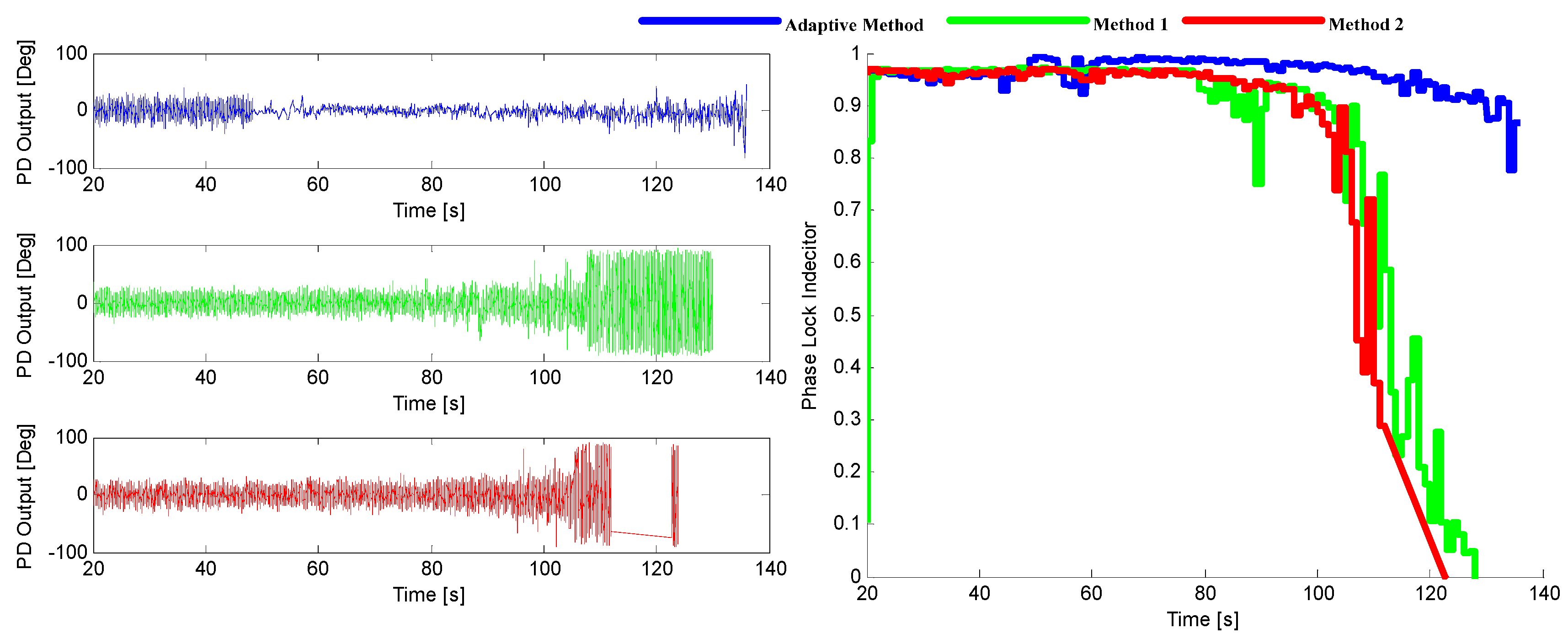
5.2. Validation of Minimum Tracking Error

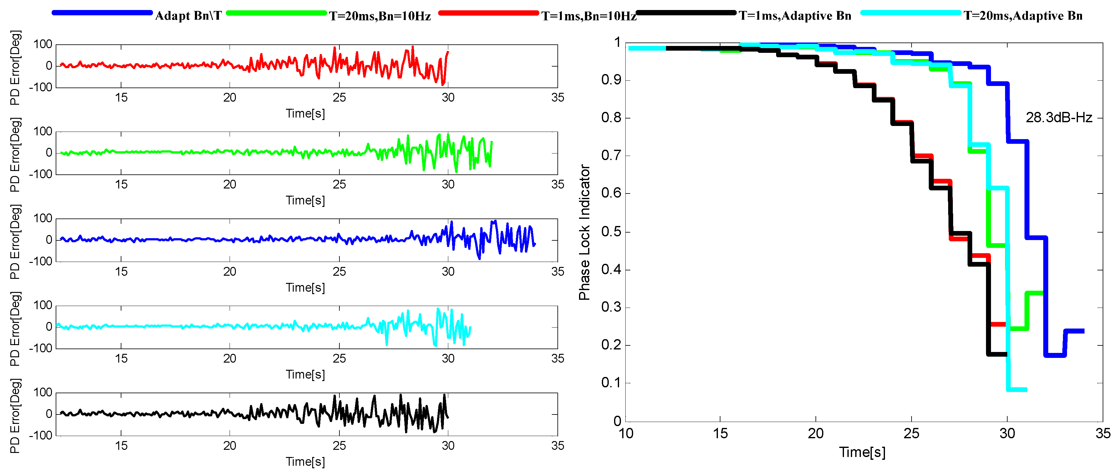
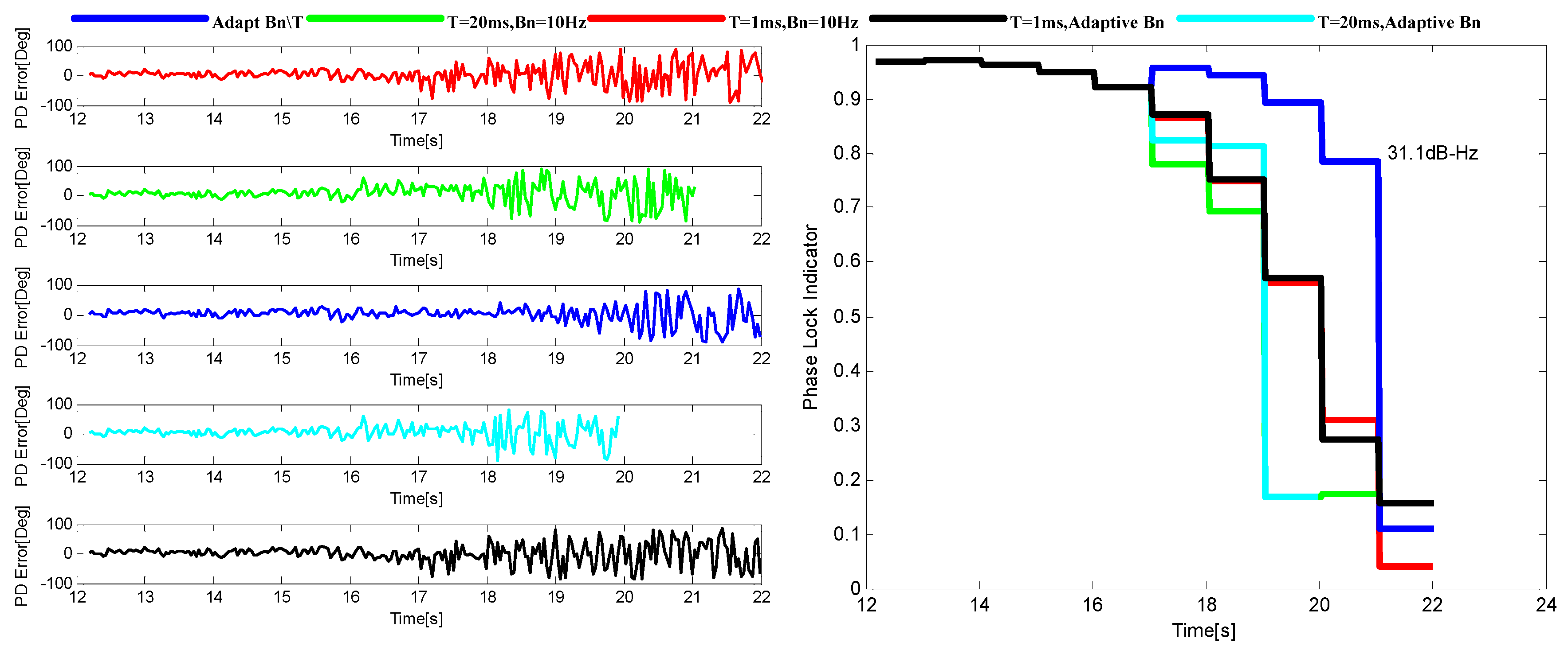
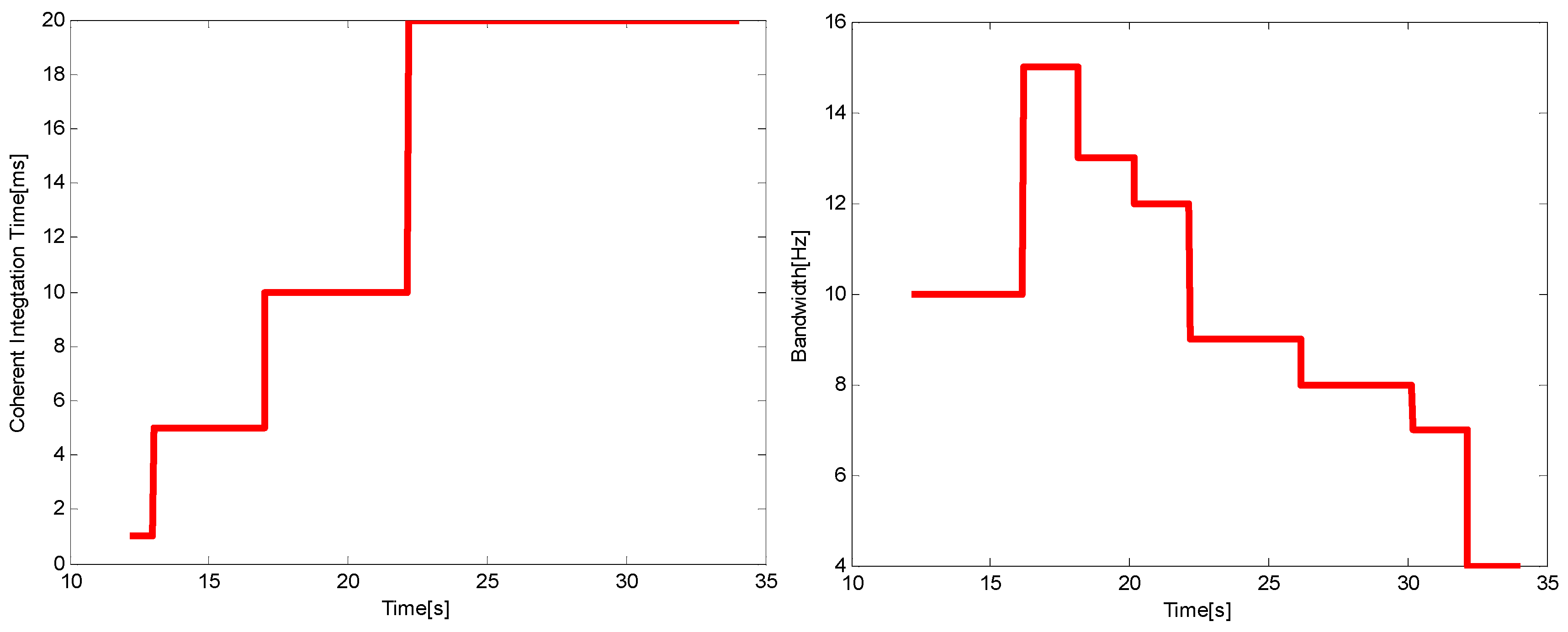
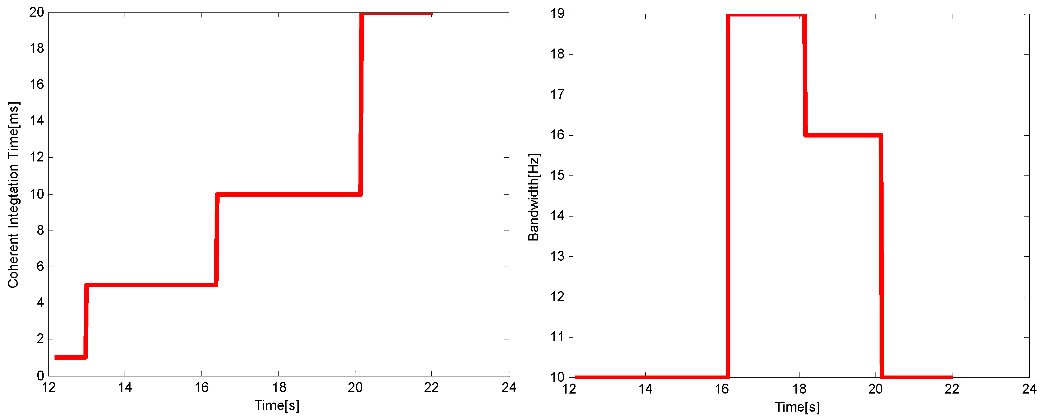
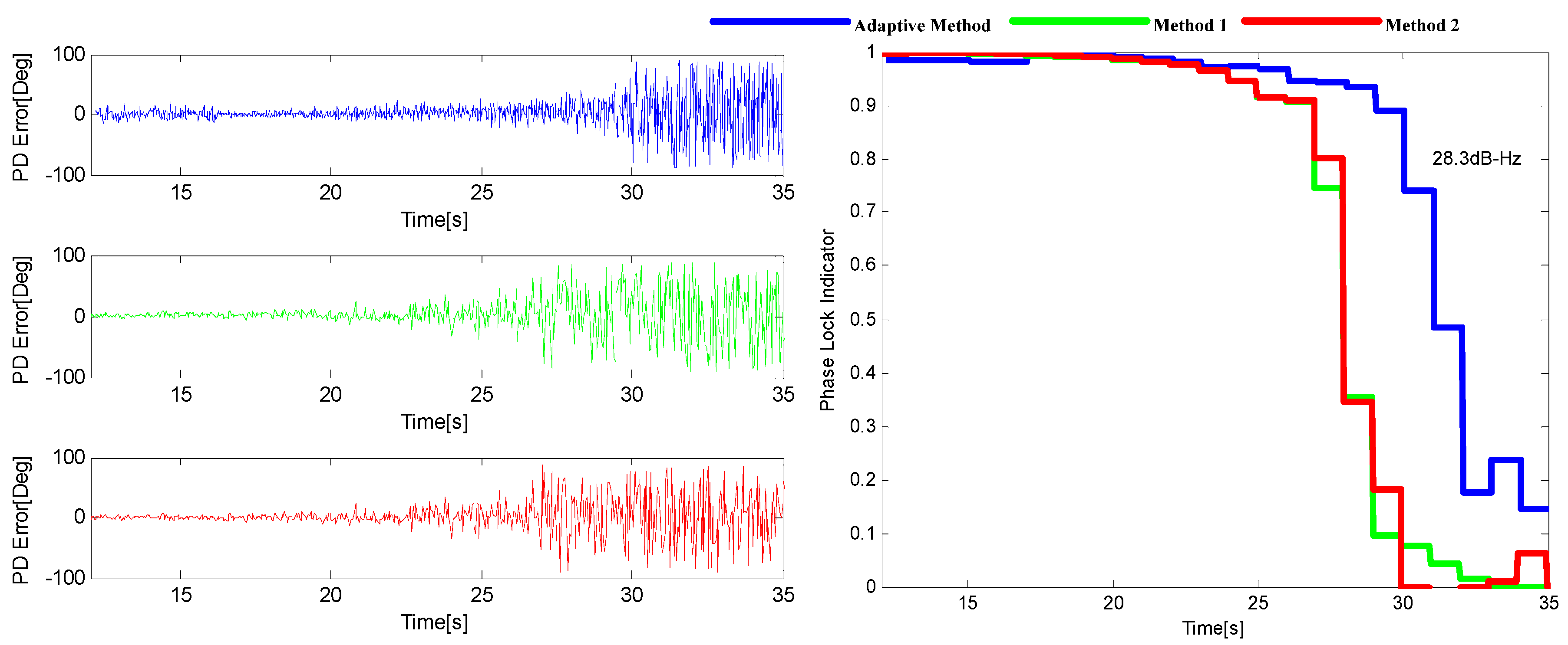
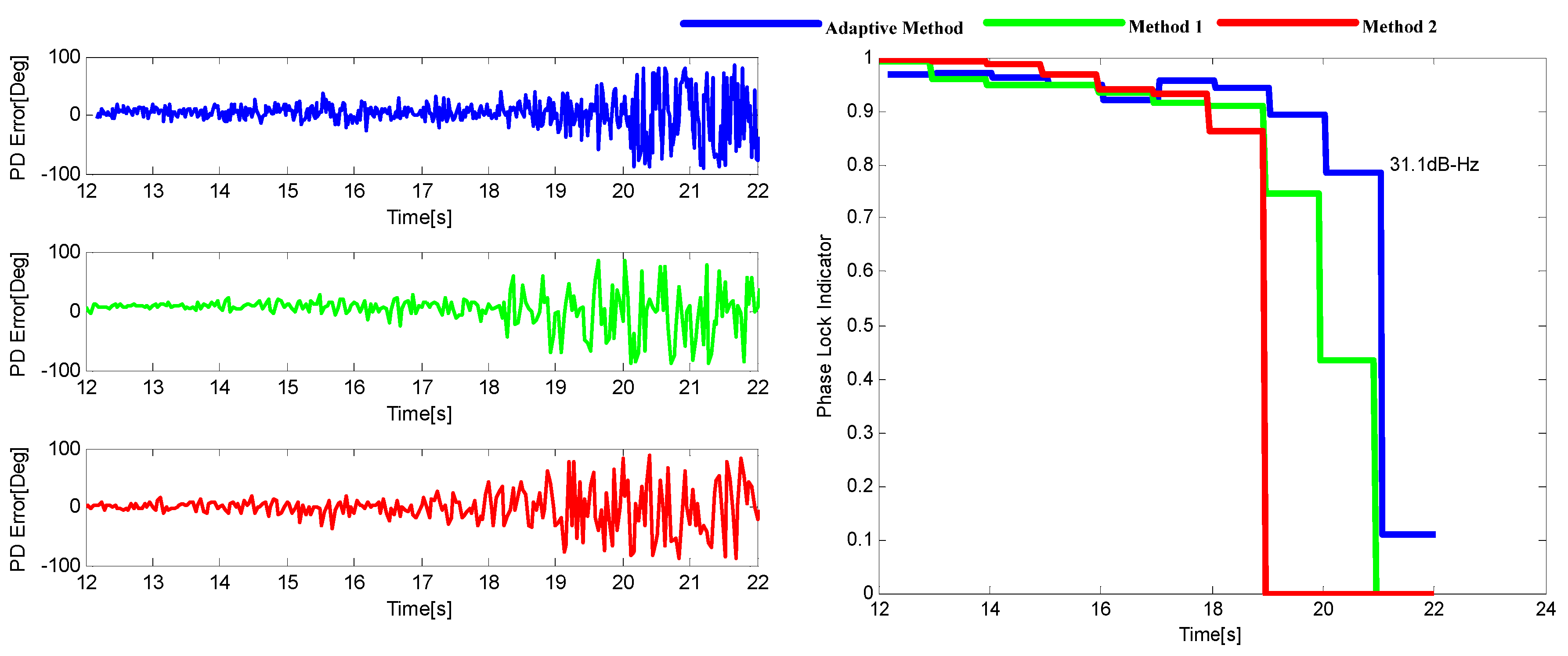
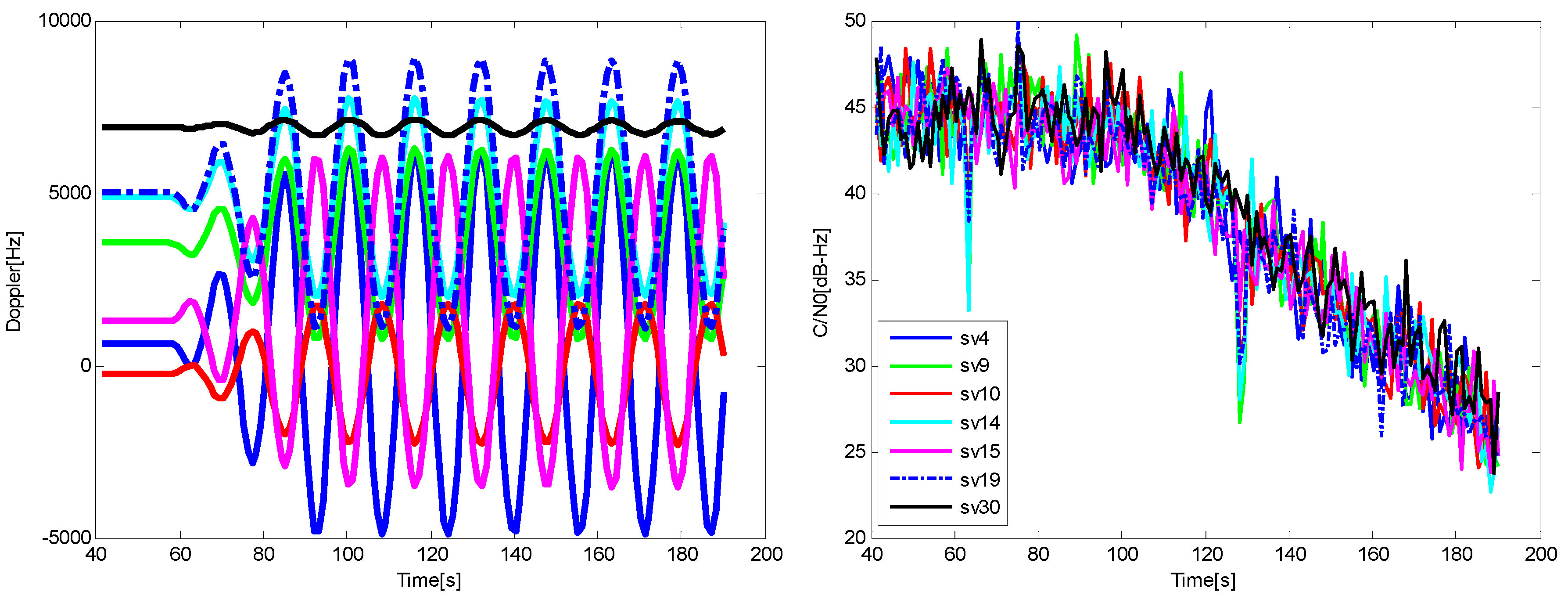
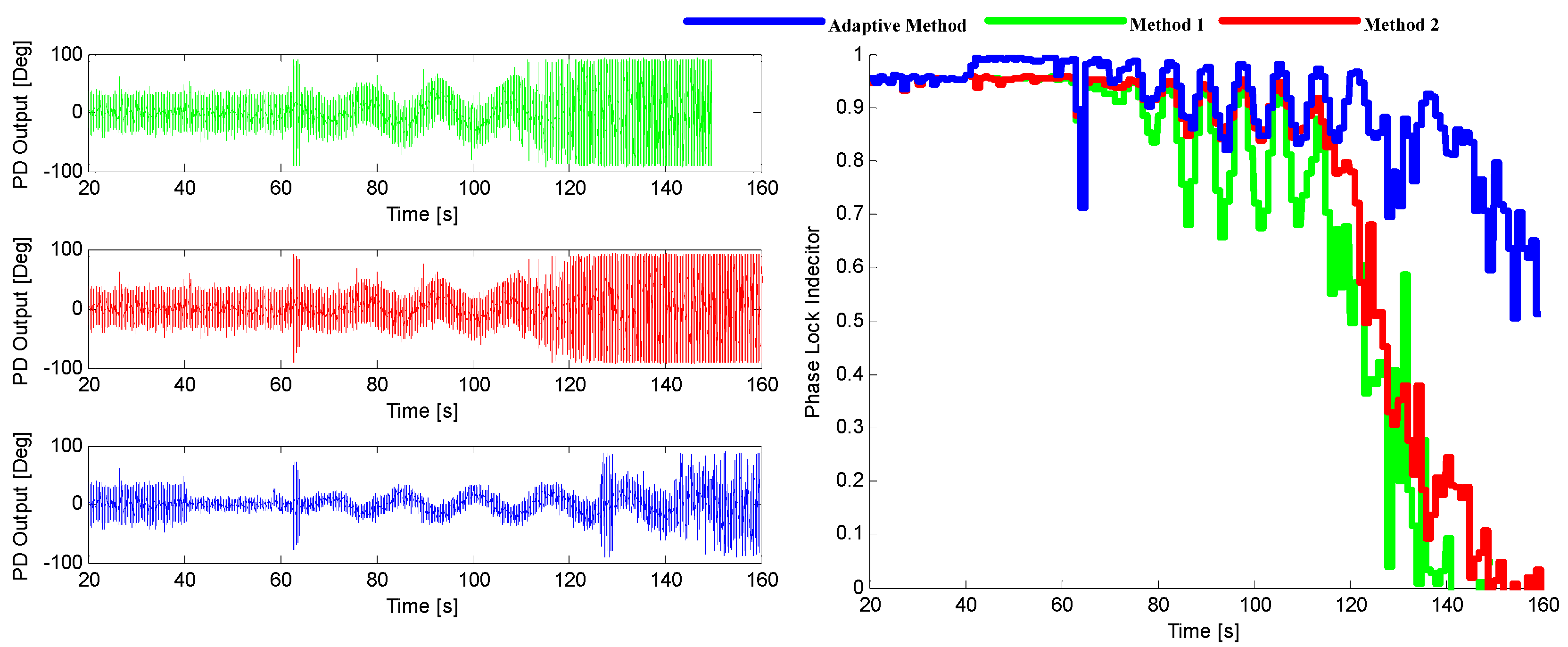
5.3. Simulation Result Analysis


| Method | Main Idea |
|---|---|
| Adaptive Method | Choose the optimal integration time and bandwidth for a given application under the minimum tracking error criterion. |
| Method 1 ([15]) | The Doppler aiding error resulting from the navigation uncertainty is derived and used to design the adaptive loop filter, so as to adjust the noise bandwidth. |
| Method 2 ([8]) | Using the fuzzy logic controller (FLC) to adjust the PLL noise bandwidth on-line. |


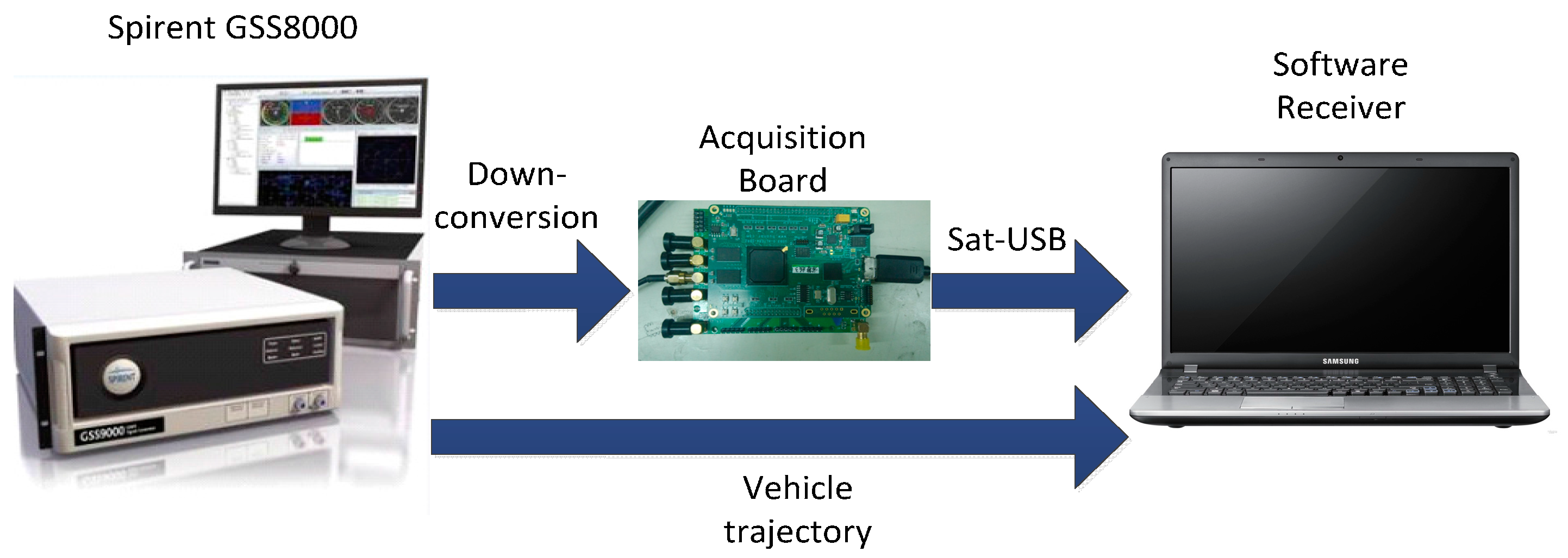
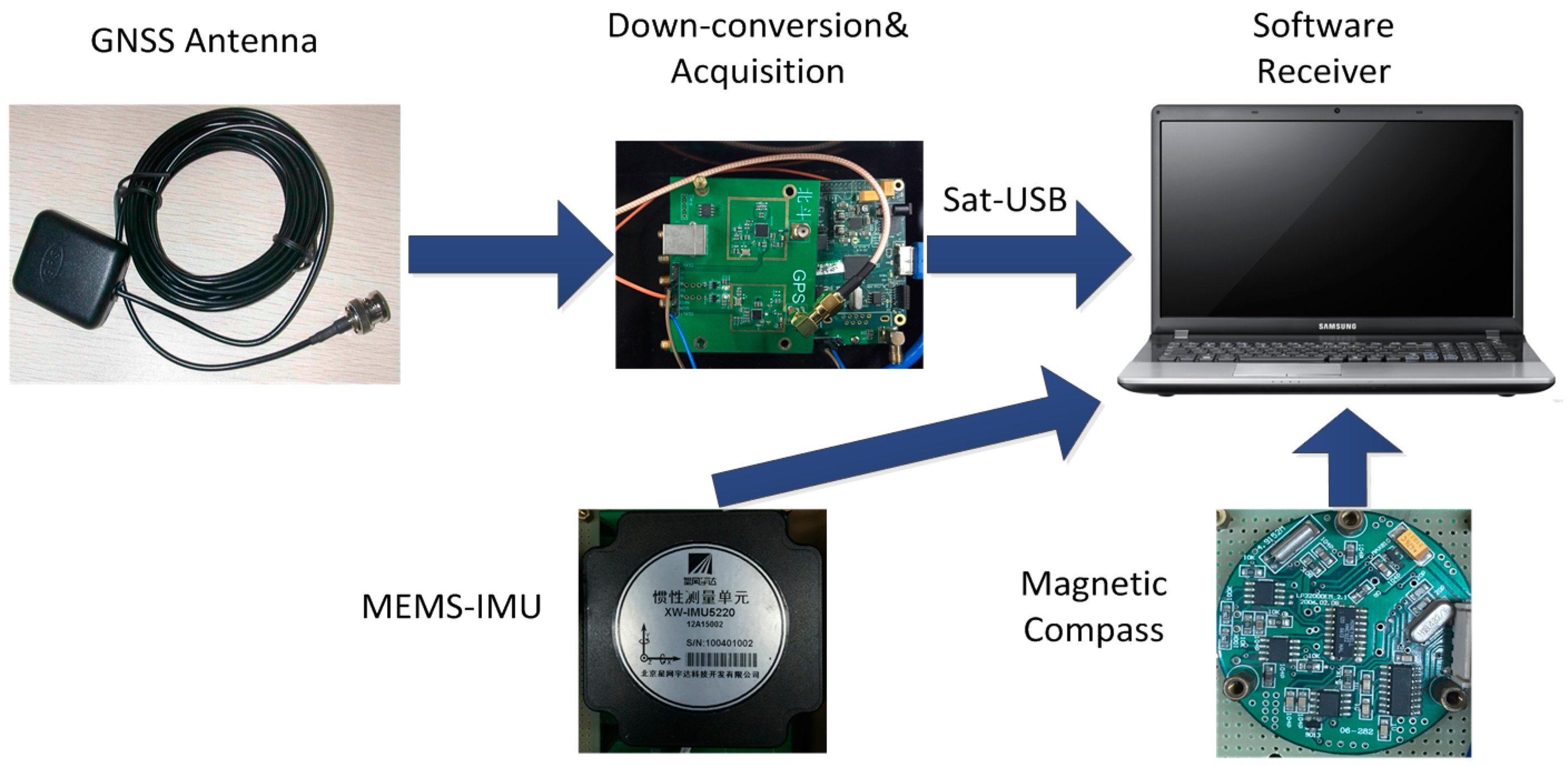
6. Hardware Simulation

6.1. The Test for the Trajectory with Lower Dynamic Condition


| Position Error (m) | Velocity Error (m/s) | |||||
|---|---|---|---|---|---|---|
| Method | Adaptive Method | Method 1 | Method 2 | Adaptive Method | Method 1 | Method 2 |
| RMS | 4.9493 | 6.4867 | 5.9646 | 0.1926 | 0.3034 | 0.3227 |
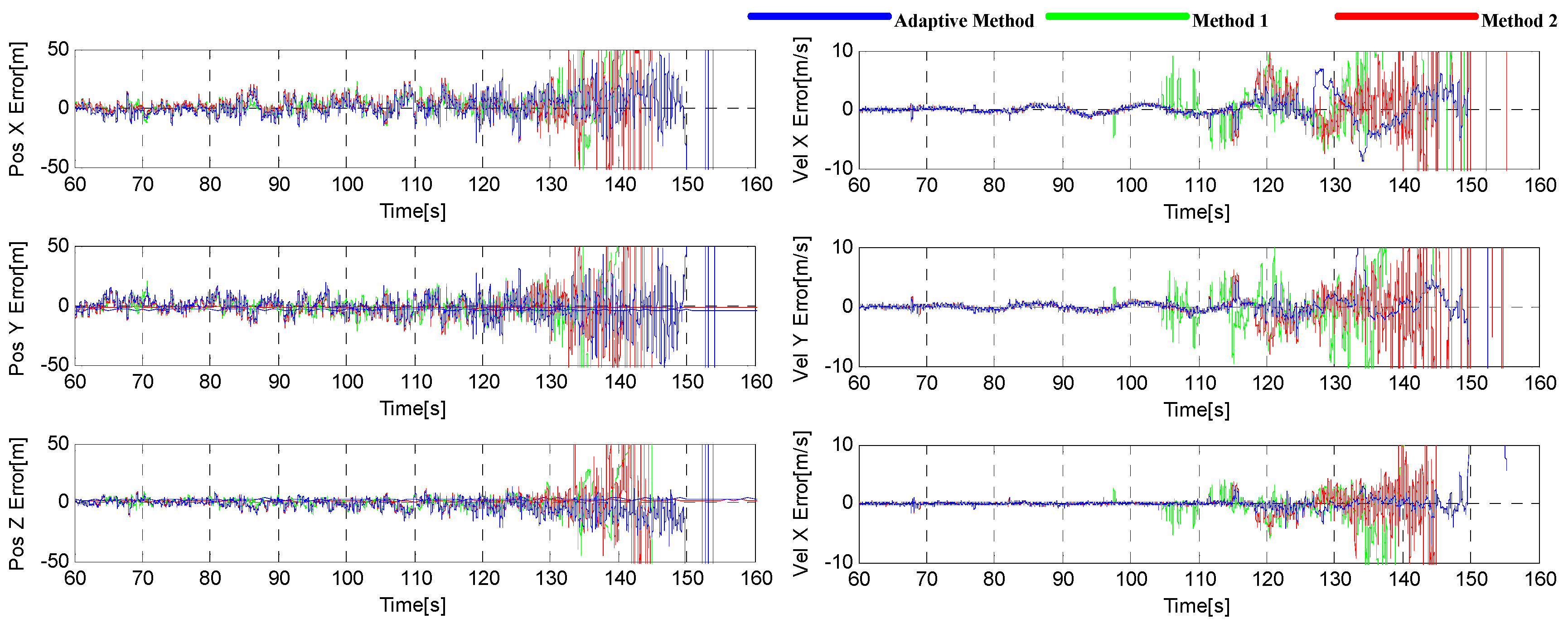
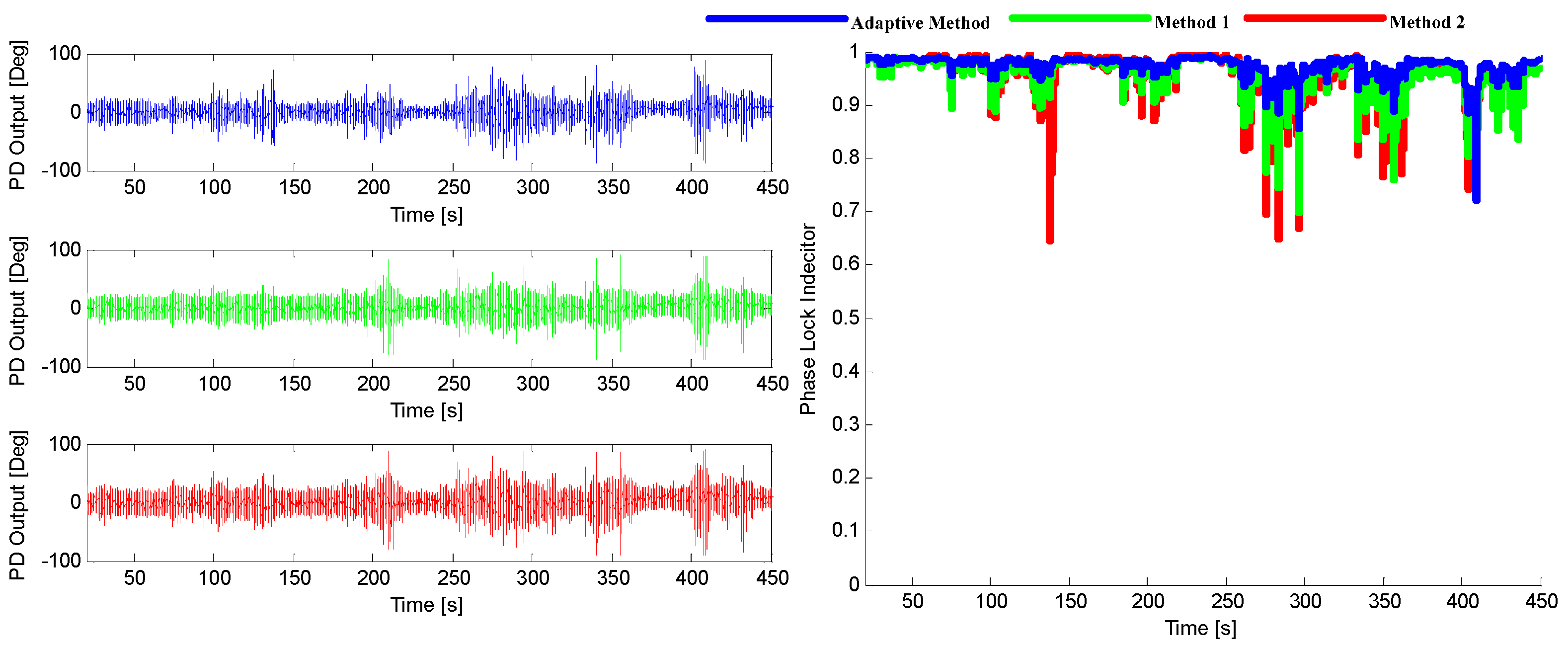
6.2. The Test for the Trajectory with Higher Dynamic Condition


| Position Error (m) | Velocity Error (m/s) | |||||
|---|---|---|---|---|---|---|
| Method | Adaptive Method | Method 1 | Method 2 | Adaptive Method | Method 1 | Method 2 |
| RMS | 8.9449 | 9.5028 | 9.5726 | 0.9431 | 1.9048 | 1.4951 |
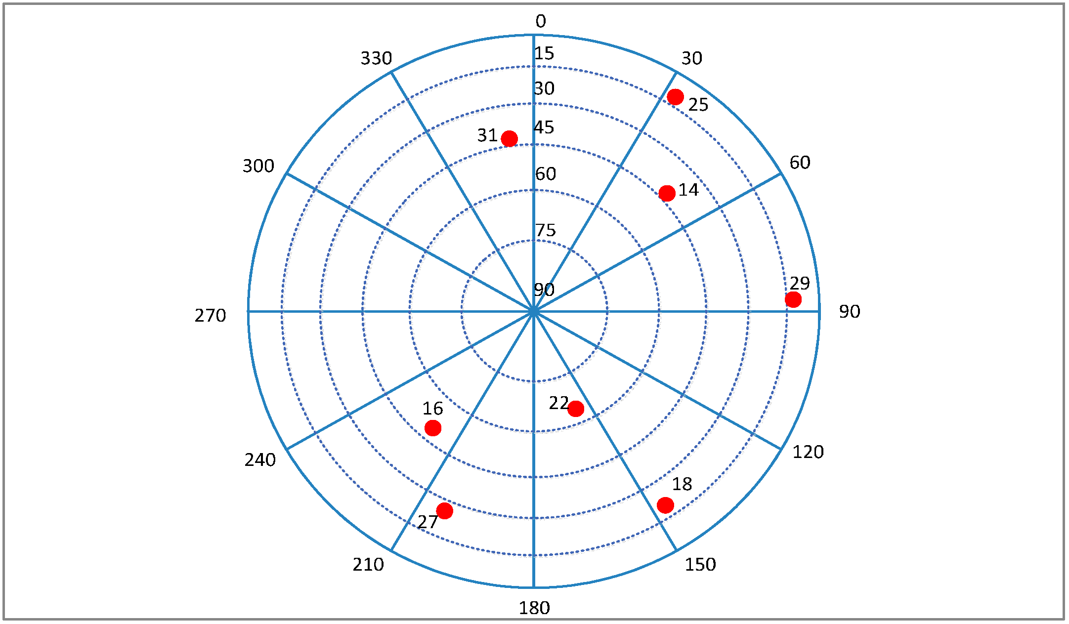
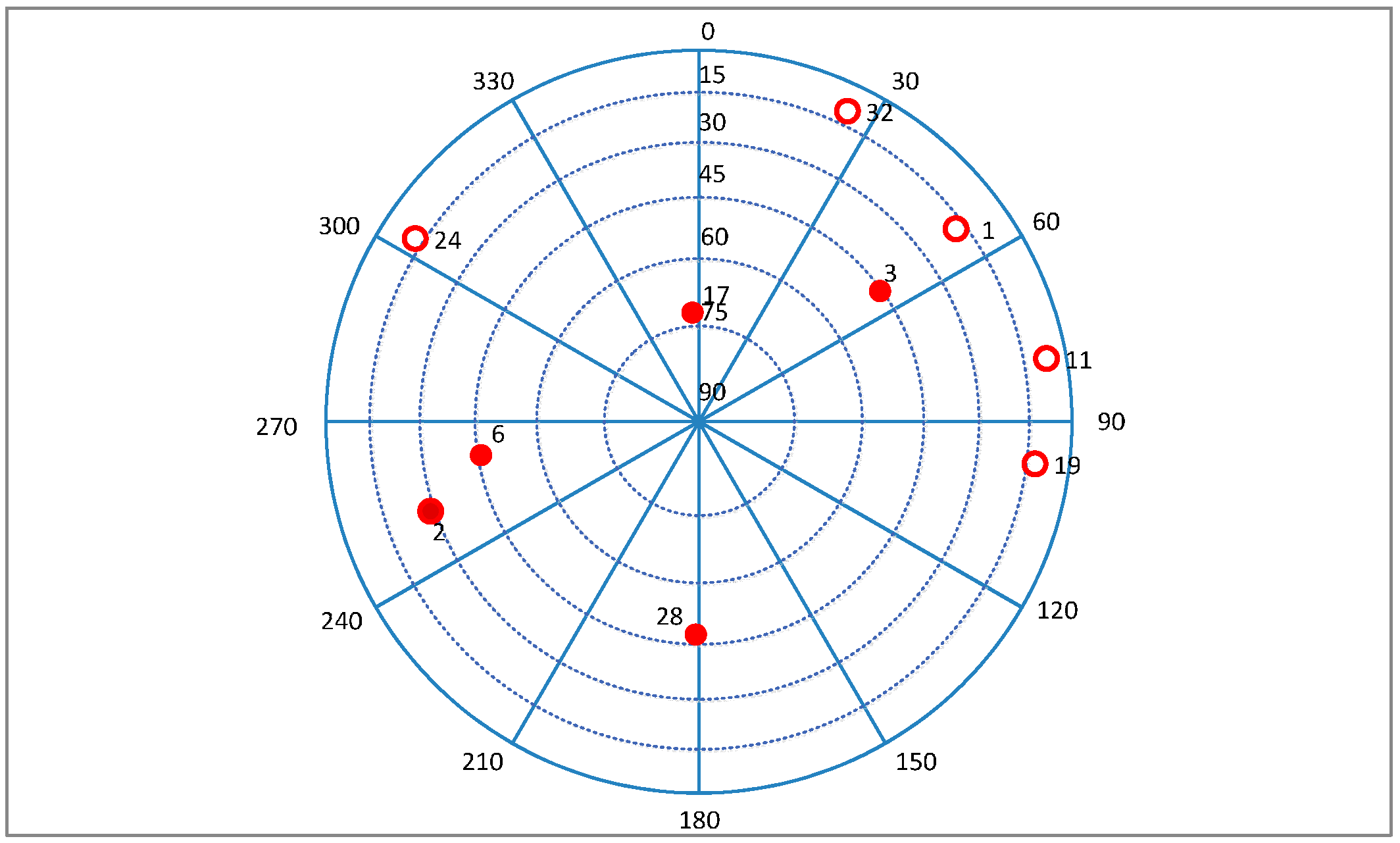
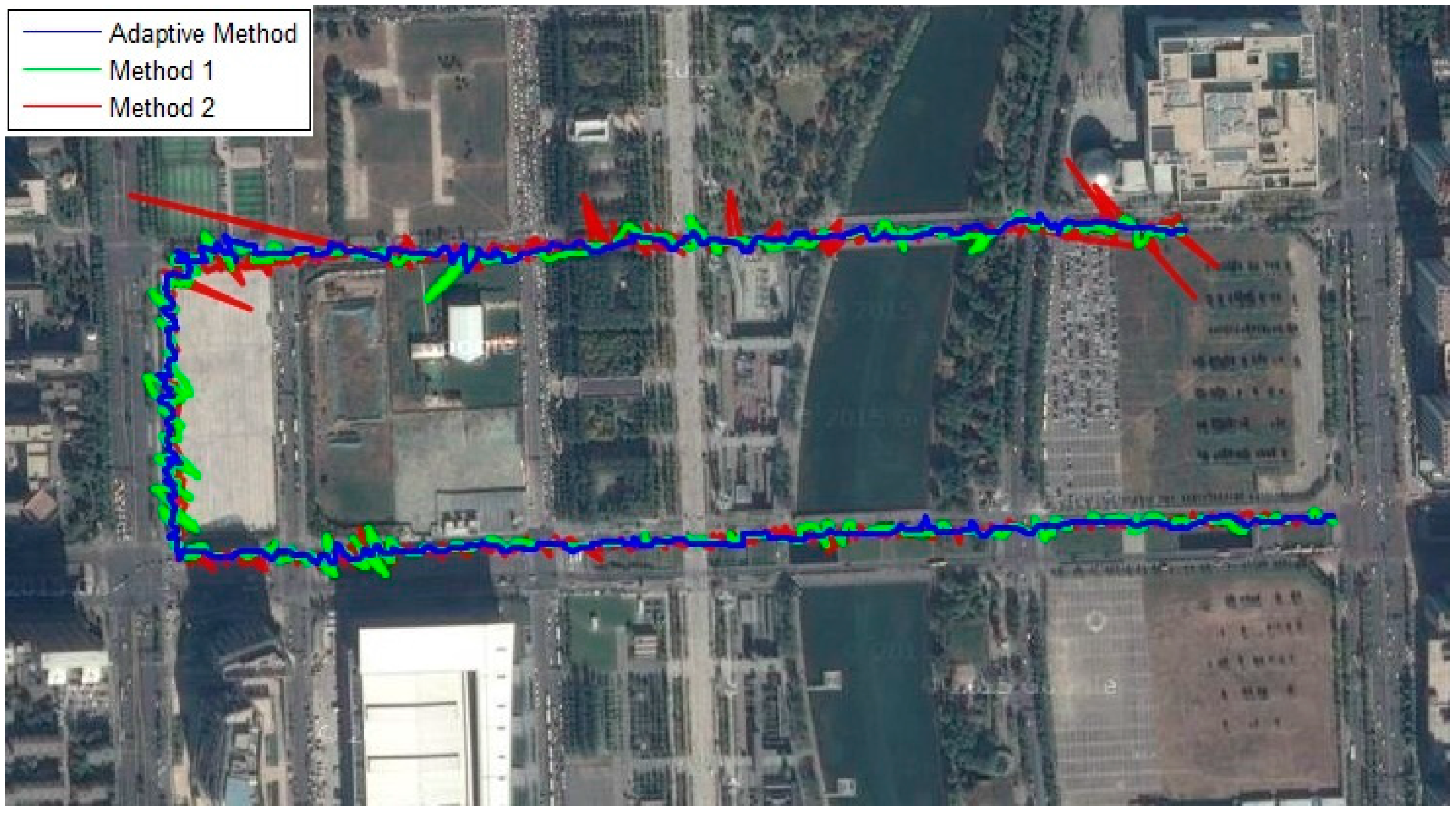
7. Field Test


8. Conclusions
Acknowledgments
Author Contributions
Conflicts of Interest
References
- El-Rabbany, A. Introduction to GPS: The Global Positioning System; Artech House: Boston, MA, USA, 2002. [Google Scholar]
- Kaplan, E.; Hegarty, C. Understanding GPS: Principles and Applications; Artech House: Boston, MA, USA, 2005. [Google Scholar]
- Wang, X.; Ji, X.; Feng, S.; Calmettes, V. A high-sensitivity GPS receiver carrier-tracking loop design for high-dynamic applications. GPS Solut. 2015, 19, 225–236. [Google Scholar] [CrossRef]
- Li, W.; Liu, S.; Zhou, C.; Zhou, S.; Wang, T. High Dynamic Carrier Tracking Using Kalman Filter Aided Phase-Lock Loop. In Proceedings of the International Conference on Wireless Communications, Networking and Mobile Computing (WiCom 2007), Shanghai, China, 21–25 September 2007; pp. 673–676.
- Han, H.; Wang, J.; Wang, J.; Tan, X. Performance Analysis on Carrier Phase-Based Tightly-Coupled GPS/BDS/INS Integration in GNSS Degraded and Denied Environments. Sensors 2015, 15, 8685–8711. [Google Scholar] [CrossRef] [PubMed]
- O’Driscoll, C.; Petovello, M.G.; Lachapelle, G. Choosing the coherent integration time for Kalman filter-based carrier-phase tracking of GNSS signals. GPS Solut. 2011, 15, 345–356. [Google Scholar] [CrossRef]
- Petovello, M.; Sun, D.; Lachapelle, G.; Cannon, M. Performance analysis of an ultra-tightly integrated GPS and reduced IMU system. In Proceedings of the 20th International Technical Meeting of the Satellite Division of The Institute of Navigation ION GNSS, Fort Worth, TX, USA, 25–28 September 2007; pp. 1–8.
- Qin, H.; Sun, X.; Cong, L. Using fuzzy logic control for the robust carrier tracking loop in a Global Positioning System/Inertial Navigation System tightly integrated system. Trans. Inst. Meas. Control 2013, 36. [Google Scholar] [CrossRef]
- Qin, F.; Zhan, X.; Du, G. Performance Improvement of Receivers Based on Ultra-Tight Integration in GNSS-Challenged Environments. Sensors 2013, 13, 16406–16423. [Google Scholar] [CrossRef]
- Razavi, A.; Gebre-Egziabher, D.; Akos, D.M. Carrier loop architectures for tracking weak GPS signals. IEEE Trans. Aerosp. Electron. Syst. 2008, 44, 697–710. [Google Scholar] [CrossRef]
- Alban, S.; Akos, D.; Rock, S.M.; Gebre-Egziabher, D. Performance analysis and architectures for INS-Aided GPS tracking loops. In Proceedings of the 2003 National Technical Meeting of The Institute of Navigation 2003, Anaheim, CA, USA, 22–24 January 2003; pp. 611–622.
- Gao, G.; Lachapelle, G. INS-assisted high sensitivity GPS receivers for degraded signal navigation. In Proceedings of the 19th International Technical Meeting of the Satellite Division of The Institute of Navigation, Fort Worth, TX, USA, 26–29 September 2006; pp. 2977–2989.
- Gebre-Egziabher, D.; Razavi, A.; Enge, P.K.; Gautier, J.; Pullen, S.; Pervan, B.S.; Akos, D.M. Sensitivity and Performance Analysis of Doppler-Aided GPS Carrier-Tracking loops. Navigation 2005, 52, 49–60. [Google Scholar] [CrossRef]
- Lian, P. Improving Tracking Performance of PLL in High Dynamic Applications. Master Thesis, University of Calgary, Calgary, AB, Canada, 2004. [Google Scholar]
- Sun, D.; Petovello, M.; Cannon, M. Use of a reduced IMU to aid a GPS receiver with adaptive tracking loops for land vehicle navigation. GPS Solut. 2010, 14, 319–329. [Google Scholar] [CrossRef]
- Patapoutian, A. On phase-locked loops and Kalman filters. IEEE Trans. Commun. 1999, 47, 670–672. [Google Scholar] [CrossRef]
- Pany, T.; Riedl, B.; Winkel, J.; Wörz, T.; Schweikert, R.; Niedermeier, H.; Lagrasta, S.; López-Risueño, G.; Jiménez-Baños, D. Coherent integration time: The longer, the better. Inside GNSS 2009, 4, 52–61. [Google Scholar]
- Tsujii, T.; Fujiwara, T.; Suganuma, Y.; Tomita, H.; Petrovski, I. Development of Ins-aided GPS tracking loop and flight test evaluation. SICE J. Control Meas. Syst. Integr. 2011, 4, 15–21. [Google Scholar] [CrossRef]
- Tawk, Y.; Tomé, P.; Botteron, C.; Stebler, Y.; Farine, P.-A. Implementation and performance of a GPS/INS tightly coupled assisted pll architecture using MEMS inertial sensors. Sensors 2014, 14, 3768–3796. [Google Scholar] [CrossRef] [PubMed]
- Zhuang, W. Performance analysis of GPS carrier phase observable. IEEE Trans. Aerosp. Electron. Syst. 1996, 32, 754–767. [Google Scholar] [CrossRef]
- Stephens, S.; Thomas, J. Controlled-root formulation for digital phase-locked loops. IEEE Trans. Aerosp. Electron. Syst. 1995, 31, 78–95. [Google Scholar] [CrossRef]
- Irsigler, M.; Eissfeller, B. PLL tracking performance in the presence of oscillator phase noise. GPS Solut. 2002, 5, 45–57. [Google Scholar] [CrossRef]
- Bhaskar, S. Exploiting quasi-periodicity in receiver dynamics to enhance GNSS carrier phase tracking. In Proceedings of the 27th International Technical Meeting of the Satellite Division of the Institute of Navigation 2014, Tampa, FL, USA, 8–12 September 2014; pp. 2563–2578.
- Jovanovic, A.; Tawk, Y.; Botteron, C.; Farine, P.-A. Multipath mitigation techniques for CBOC, TMBOC and ALTBOC signals using advanced correlators architectures. In Proceedings of the 2010 IEEE/ION Position Location and Navigation Symposium (PLANS), Indian Wells, CA, USA, 4–6 May 2010; pp. 1127–1136.
- GSS8000 Multi-GNSS Constellation Simulator. Available online: http://www.spirent.com/Solutions-Directory/GSS8000 (accessed on 26 August 2015).
© 2016 by the authors; licensee MDPI, Basel, Switzerland. This article is an open access article distributed under the terms and conditions of the Creative Commons by Attribution (CC-BY) license (http://creativecommons.org/licenses/by/4.0/).
Share and Cite
Cong, L.; Li, X.; Jin, T.; Yue, S.; Xue, R. An Adaptive INS-Aided PLL Tracking Method for GNSS Receivers in Harsh Environments. Sensors 2016, 16, 146. https://doi.org/10.3390/s16020146
Cong L, Li X, Jin T, Yue S, Xue R. An Adaptive INS-Aided PLL Tracking Method for GNSS Receivers in Harsh Environments. Sensors. 2016; 16(2):146. https://doi.org/10.3390/s16020146
Chicago/Turabian StyleCong, Li, Xin Li, Tian Jin, Song Yue, and Rui Xue. 2016. "An Adaptive INS-Aided PLL Tracking Method for GNSS Receivers in Harsh Environments" Sensors 16, no. 2: 146. https://doi.org/10.3390/s16020146