
Fusion of Multispectral Imagery and Spectrometer Data in UAV Remote Sensing


1
Department of Geography and Environmental Studies, Carleton University, 1125 Colonel By Dr., Ottawa, ON K1S 5B6, Canada
2
A&L Canada Laboratories, 2136 Jetstream Rd., London, ON N5V 3P5, Canada
*
Author to whom correspondence should be addressed.
Remote Sens. 2017, 9(7), 696; https://doi.org/10.3390/rs9070696
Submission received: 24 April 2017
/
Revised: 13 June 2017
/
Accepted: 2 July 2017
/
Published: 6 July 2017
Abstract
:High spatial resolution hyperspectral data often used in precision farming applications are not available from current satellite sensors, and difficult or expensive to acquire from standard aircraft. Alternatively, in precision farming, unmanned aerial vehicles (UAVs) are emerging as lower cost and more flexible means to acquire very high resolution imagery. Miniaturized hyperspectral sensors have been developed for UAVs, but the sensors, associated hardware, and data processing software are still cost prohibitive for use by individual farmers or small remote sensing firms. This study simulated hyperspectral image data by fusing multispectral camera imagery and spectrometer data. We mounted a multispectral camera and spectrometer, both being low cost and low weight, on a standard UAV and developed procedures for their precise data alignment, followed by fusion of the spectrometer data with the image data to produce estimated spectra for all the multispectral camera image pixels. To align the data collected from the two sensors in both the time and space domains, a post-acquisition correlation-based global optimization method was used. Data fusion, to estimate hyperspectral reflectance, was implemented using several methods for comparison. Flight data from two crop sites, one being tomatoes, and the other corn and soybeans, were used to evaluate the alignment procedure and the data fusion results. The data alignment procedure resulted in a peak R2 between the spectrometer and camera data of 0.95 and 0.72, respectively, for the two test sites. The corresponding multispectral camera data for these space and time offsets were taken as the best match to a given spectrometer reading, and used in modelling to estimate hyperspectral imagery from the multispectral camera pixel data. Of the fusion approaches evaluated, principal component analysis (PCA) based models and Bayesian imputation reached a similar accuracy, and outperformed simple spline interpolation. Mean absolute error (MAE) between predicted and observed spectra was 17% relative to the mean of the observed spectra, and root mean squared error (RMSE) was 0.028. This approach to deriving estimated hyperspectral image data can be applied in a simple fashion at very low cost for crop assessment and monitoring within individual fields.

1. Introduction
Hyperspectral sensors with many narrow spectral bands have been shown to be able to characterize vegetation type, health, and function [1,2,3,4]. Compared with multispectral imagery, hyperspectral data were reported to perform better in modelling vegetation chlorophyll content [5]. They can also be used to calculate narrow band indices for modelling crown temperature, carotenoids, fluorescence, and plant disease [6,7], as well as crop growth period [8], soil status [9], net photosynthesis, and crop water stress [10], amongst other vegetation parameters. In precision farming applications, hyperspectral data with high spatial resolution are required [4,11], but such data are currently not available from satellite sensors. Hyperspectral sensors designed for standard aircraft are generally expensive, and such aircraft require significant infrastructure, maintenance, and personnel resources.
Unmanned aerial vehicles (UAVs) are a rapidly evolving and flexible platform for remote sensing. They offer a promising alternative to standard aircraft in terms of timing flexibility and capability to fly at very low altitudes, thereby acquiring imagery of very high spatial resolution. Small, low cost UAVs are particularly advantageous for applications in small individual farm management. The improvement of such UAV platforms and the miniaturization of sensors have stimulated much remote sensing research and the development of new systems [12]. For example, Jaakkola, et al. [13] developed a multiple sensor platform, with the spectrometer and GPS units weighing 3.9 kg. More recently, hyperspectral sensors of about 2 kg or less have been developed for small UAVs [14,15].
When the total system requirements are considered, however, hyperspectral imaging systems are often too expensive and complicated for small applications-based companies or individual farmers without aviation and remote sensing systems expertise. Besides the sensor itself, the payload requirements also generally include accurate GPS/IMU instrumentation, and an on-board computer for effective data collection. These, combined with other sensors such as a standard RGB camera, may necessitate a larger and more expensive UAV platform, driving up system costs. In addition, hyperspectral sensors acquire data in pushbroom or whiskbroom mode, one image line at a time. The image geometry is therefore more affected by UAV rotations than for a frame camera, which acquires imagery over a two dimensional space in each exposure. The post-acquisition data processing and cost to correct such line-by-line geometric distortions is therefore significant with hyperspectral sensors.
To develop a means for low cost and simplified acquisition of hyperspectral data, this study took an alternative approach. The goal was to fuse the high spectral information content of a low cost miniature spectrometer with the high spatial information content of a low cost multispectral camera system. Using a spectrometer alone in a UAV can provide excellent spectral information [16], but it can only collect samples of a limited number of ground locations, and the footprint in which radiance is collected does not contain explicit spatial information as in a raster image. By exploiting the relationship between such sample-based spectrometer measured spectra, and image data from a frame-based multispectral sensor, hyperspectral data can be estimated at all locations (pixels) in the image where spectrometer data do not exist, thereby deriving an estimated hyperspectral image. The estimated hyperspectral image is in a 2D frame format, which eliminates the need for the geometric processing required for standard hyperspectral line sensors. Moreover, such a system has the potential to cost a fraction of current UAV-based hyperspectral systems and reuse existing cameras and equipment.
Challenges of data collection via multiple low cost sensors include sensor calibration, alignment and data processing. Calibration of UAV hyperspectral sensor data has been conducted using calibration targets in the field [17,18], and lab-based spectrometry with lamp reference sources [19], to evaluate the accuracy of observed hyperspectral data and the dominant noise sources, such as dark current, sensor temperature, atmosphere, and weather [20]. Sensor alignment has been a consideration for multiple sensors of the same type [21], and for different sensors [22]. In low cost UAV multiple sensor systems, it is not easy, or possible, to optically align sensors in a mount that will maintain the precise alignment in the field over multiple flight hours. Thus, matching data from multiple sensors requires post-flight consideration of their spatial misalignment, as well as their data–rate timing differences. Once data alignment from the two sensors has been achieved, fusion can be accomplished by using coincident data from both sensors (i.e., data acquired at the same locations) as training data to build a model. Subsequently, the model can be used to estimate hyperspectral reflectance at other locations where only the multispectral camera has acquired data.
The objectives of this research were to develop methods for (1) alignment of data collected from a spectrometer and a multispectral camera system, (2) fusion of these two data types to provide estimated hyperspectral data at each pixel in the multispectral camera imagery.
2. Methodology
2.1. The Conceptual Framework of Data Acquisition and Fusion
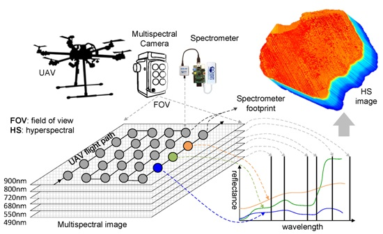
The remote sensing system for the proposed data fusion process includes a multispectral imaging sensor and a spectrometer; for our purposes, they are mounted on a small UAV as shown in Figure 1, but they could be mounted on any in situ or airborne platform. Mounting the two sensors is conducted to visually achieve alignment of their optical axes (e.g., with the spectrometer and camera housings parallel). The multispectral sensor acquires 2D multiple band images from separate cameras, each with a specific bandpass filter, while the spectrometer collects one full spectrum sample per measurement within a near circular footprint determined by the angle of view (optics) and the platform altitude and orientation. The details of our experimental UAV system, settings and camera configuration are further described in Section 3. Given an appropriate frame rate or GPS-controlled camera triggering is used, the multispectral camera images should cover the required area; for most applications a mosaic must be produced from multiple images. The spectrometer samples will cover a set of footprints, each being much larger than the multispectral image pixels, and these footprints may not cover the whole study area, due to the spectrometer data rate and UAV velocity. The goal is to associate individual reflectance measurements from the 1D spectrometer, with pixels in the 2D multispectral images that fall within the field of view of the spectrometer. The approach taken in this study was to develop post-acquisition processing methods to optimize the alignment of the data from the two sensors, by evaluating their timing and spatial correlations. Details are provided in Section 2.2.
Once data alignment has been optimized, fusion of the two data types is conducted by cross calibrating coincident sample points of full spectrum spectrometer data and multispectral image data, and using that relationship to estimate full spectrum reflectance at all pixels in the multispectral camera images. Many spectra acquired by the spectrometer are selected to build a training dataset of representative ground features (e.g., soil, corn, wheat). A small proportion of the measured spectra can be set aside as independent reference data to assess the accuracy of the estimated hyperspectral imagery. More details about the data fusion methods are explained in Section 2.3.
2.2. Alignment of Spectrometer and Multispectral Camera Data
The data from the two sensors need to be aligned before fusion is implemented, due to misalignment caused by sensor timing differences and inclined optical axes. This study assumes that the highest data correlation should be found when the multispectral camera and spectrometer data are optimally aligned. Since data misalignment occurs in both the time domain and spatial domain, this study employs a global alignment procedure that considers both time and space offsets simultaneously.
Spectrometer data are acquired in raw format as arbitrary intensity units. A white barium sulfate disc representing close to 100% Lambertian reflectance is used before and after flights to measure reference intensity. Reflectance of ground targets is calculated as
where is nominal surface reflectance, is wavelength, I is the radiance intensity recorded by the spectrometer for ground target surfaces (S) and the white reference (R), respectively. Dark noise (measured with the lens cap on) is subtracted from all intensity readings I at each wavelength before reflectance is calculated. A second skyward pointing spectrometer attached with cosine corrector (180° field of view or “FOV”) that can be on the UAV or on the ground (to minimize UAV weight) measures downwelling irradiance. Nominal reflectance is further adjusted for illumination conditions as measured by the skyward pointing spectrometer:
where E is the downwelling irradiance [23] measured by the skyward spectrometer. E(S) and E(R) are measured at the same time as the air-unit intensity (I) measurements of the target surfaces (S) and white reference (R), respectively. The sum of irradiance over all wavelengths as a coefficient is used to represent the total sun irradiance at a given moment.
For the multispectral sensor, each spectral band has a transmittance function over a wider range of wavelengths than the spectrometer bands. For instance, the red band of the camera used in this study is centered at 680 nm, with a Gaussian transmittance distribution between 660 and 700 nm [24]. To make the reflectance of the multispectral data comparable to the spectrometer data, a convolution of the spectrometer reflectance over the wavelength range of each multispectral band is required:
where is the nominal convoluted reflectance corresponding to multispectral band b, and Tb(λ) is the transmittance function over band b within the wavelength range λmin to λmax.
In addition, the spectrometer footprint approximates a circle on the ground that covers multiple pixels of the multispectral image, as illustrated in Figure 2. To produce spatially comparable data, the mean of the multispectral imagery pixel intensity values (V) within the spectrometer footprint is calculated:
where V is the multispectral image pixel value (intensity), (x, y) and (i, j) are image coordinates using the multispectral image center as the origin, dist is the 2D distance based on X and Y directions, and n is the number of pixels within the given footprint area of radius r. In nadir view, assuming UAV rotations are negligible, r is constant for a given flight where the sensors are mounted at fixed positions on the UAV.
Following the above steps, the acquired signals from the multispectral camera and spectrometer are comparable spectrally and spatially. The correlation (determination coefficient, R2) between the two data sets is then calculated to determine the best alignment; i.e., the alignment for which the R2 between the datasets is maximized (Equation (5)).
where the f is the linear correlation with its coefficient of determination R2, ρb and V were as previously defined. Note that while ρb is reflectance and V intensity, their relationship is linear, so V does not have to be converted to reflectance to be correlated against ρb. Δt is the misalignment due to time offset of the sensors, and Δθ is the view angle misalignment between the sensors. Both contribute to the offset of the spectrometer footprint in the horizontal and vertical directions (Δx, Δy) from the multispectral image center. This misalignment in both time and spatial domains (Δt, Δθ), expressed as (Δt, Δx, Δy), is optimized simultaneously.
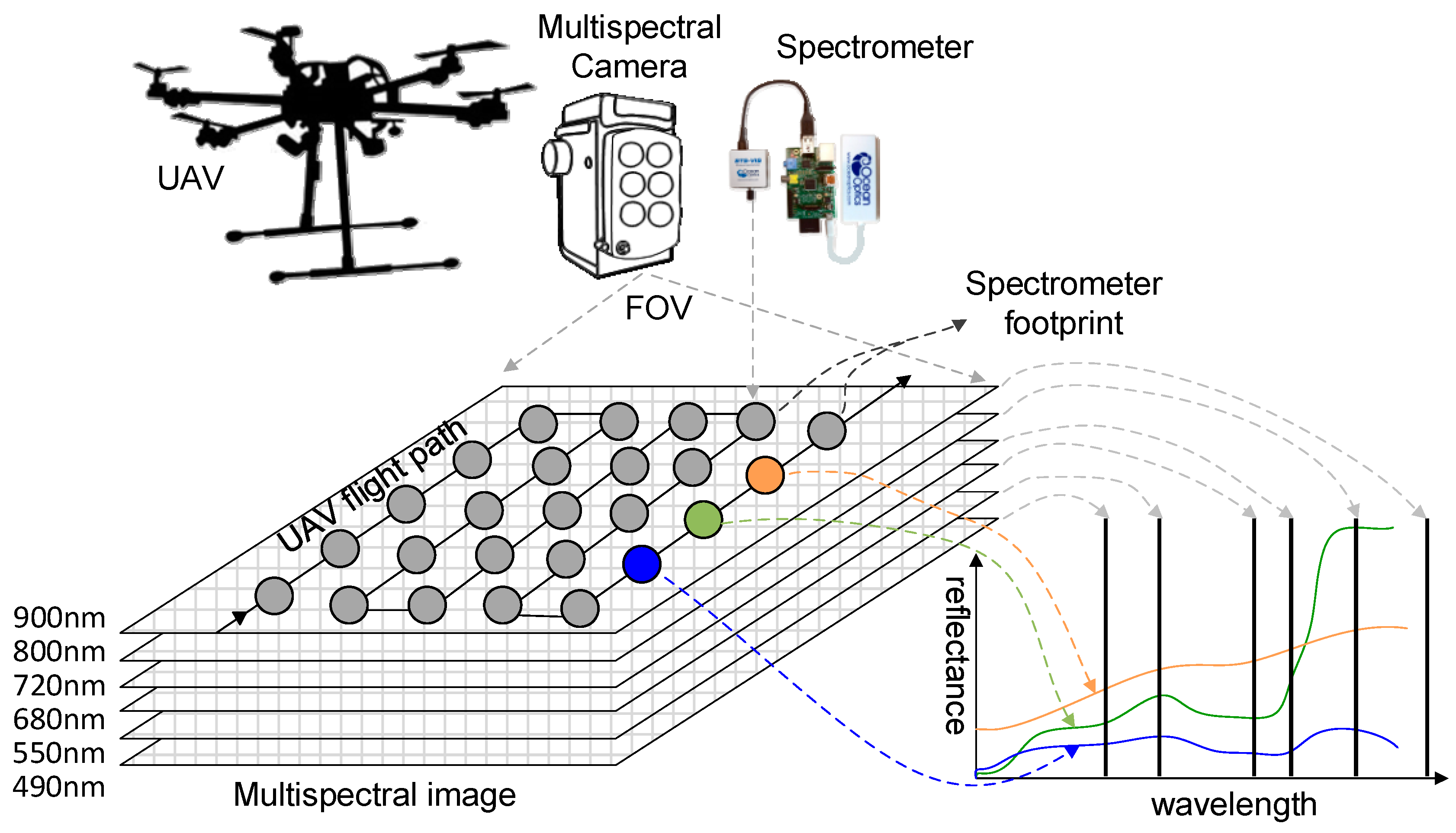
Reasonable search ranges for both the time and space domains are initially set for the optimization. The time domain search range is defined as the time shift from the initial multispectral camera–spectrometer data match according to their nominal time tags; 10 s before and after this initial match was used in this study. As illustrated in Figure 2, the method uses the time of multispectral images as the base, while shifting the timeline of spectrometer data in steps equal to the spectrometer data collection interval (0.2 s). In the space domain, the search range is defined around the multispectral camera image center. A search range at an interval of 5 pixels (about 8 cm) in both the X and Y directions out to ±100 pixels from the multispectral image center was defined. For each interval in the search ranges of both the time and space domains, R2 was calculated; the maximum R2 within the searching range according to Equation (5) corresponds to the optimized time offset from its initial matched time (Δt) and the optimized spatial offset from the multispectral camera image center (Δx, Δy).
2.3. Fusion of Spectrometer and Multispectral Camera Data
Suppose represents the intensity recorded by the multispectral camera in m spectral bands, and represents the reflectance recorded by the spectrometer in n bands; observation of a given location with both the multispectral camera and the spectrometer can be expressed as
After a flight, each location on the ground is covered by a multispectral camera pixel, thus is known for all l ground locations. However, there is only a limited number of k locations represented by the spectrometer measurements. The measurement matrix for a flight Obs, is therefore comprised of pairs of measurement locations to , as well as multispectral camera measurements to , for which there are no spectrometer measurements, as shown in Equation (7):
The first k measurements from both sensors can be used as training data to predict the unknown spectral reflectance in the remaining (l − k) ground (pixel) locations, where only exists. Methods to estimate hyperspectral reflectance at unknown locations in recent studies include spline interpolation [25,26], Bayesian imputation [8,27], missing data imputation methods [28,29] based on principal component analysis (PCA), and others. Spline interpolation simply exploits the high correlation between spectral bands to interpolate the hyperspectral band reflectance from the limited number of multispectral bands. Bayesian estimation [8,27] assumes that, given the a priori covariance of the hyperspectral bands, a full spectra can be inferred from the multispectral imagery using Bayesian imputation. Bayesian imputation estimates a missing hyperspectral value as the mean value of the predictive based on a posterior conditional distribution (hyperspectral conditional on multispectral). The PCA-based data imputation method selected for this study, compresses the data into a few explanatory latent variables, and imputes unknown hyperspectral reflectance based on the latent structure of the data set [28,29,30]. Specifically, PCA-based imputation methods first calculate a PCA model from both multispectral and hyperspectral data (unknown hyperspectral data are filled with zeros in this stage); this PCA will then be employed to impute and replace unknown hyperspectral bands with known multispectral data as input. Iteration is then carried out until the difference between the newly imputed hyperspectral data and the previous ones are smaller than a specified tolerance, thus indicating convergence.
This study implemented these three groups of fusion methods. In the PCA methods, we tested slightly different methods as defined in [29], including trimmed scores regression (TSR), known data regression (KDR), known data regression with principal component regression (KDR–PCR), KDR with partial least squares regression (KDR–PLS), projection to the model plane (PMP), filling in the missing data with the predictions obtained from previous PCA models iterated recursively until convergence (IA), modified nonlinear iterative partial least squares regression algorithm (NIPALS), and data augmentation (DA). In the Bayesian methods, three different approaches to perform stochastic sampling: Gibbs, expectation maximization (EM), and iterative conditional modes (ICM), were employed to estimate hyperspectral data based on multivariate normal distribution and maximum likelihood estimation [27].
Apart from these three categories of hyperspectral prediction approaches, there have been many studies on the data fusion of hyperspectral imagery and multispectral imagery (e.g., [31,32]). Hyperspectral–multispectral (HS–MS) image fusion, however, is a different problem from the hyperspectral prediction studied here. In HS–MS data fusion, and are both known for all locations in the image but with different spatial resolution. By contrast, in this study, is known at all pixels, but exists only at a set of sample locations within the image (Figure 1 and Figure 2).
3. Study Site, UAV System, and Flight Design
3.1. Study Site
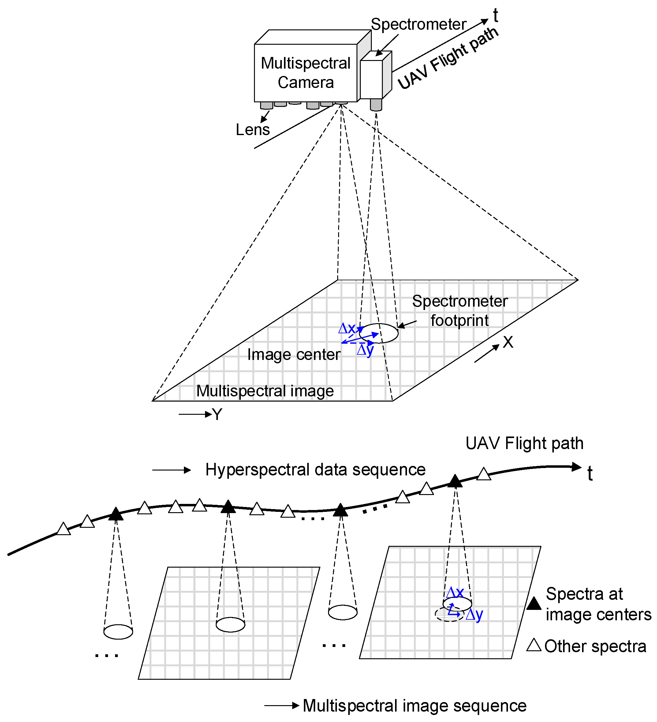
In the application and evaluation of the data fusion approach, UAV flights were conducted over an experimental farm on 21 July 2016, near London Ontario, Canada. A hexa-copter (DJI Spreading Wings S800) was used with take-off weight (including sensors) of 6 kg. For the lightweight sensors used in this study (Section 3.2), an even smaller and lower cost UAV could be used. The major ground cover types were crops, bare soil, and gravel roads, with smaller extents of other short vegetation, trees and buildings. The planned and actual UAV flight paths are shown in Figure 3a,b, where two flights were conducted over a tomato field (Site 1), and a larger field of corn and soybean (Site 2), respectively. The flight speed was 5 m/s, and the flight altitude was 30 m and 50 m above ground for Site 1 for Site 2, respectively. The sky was clear during the flights with negligible sun illumination variation.
3.2. UAV Spectrometer and Multispectral Camera Systems
The UAV spectrometer was an Ocean Optics STS–VIS model, which is 40 mm × 42 mm × 24 mm and weighs 60 g. It has a 1024 bands, each of 0.46 nm full bandwidth, over the spectral range from about 350 nm to 800 nm. The FOV was 1.5° using a fiber optic cable (length: 25 cm, core size: 400 μm) and collimating lens. The integration time is manually set between 100 ms and 1000 ms (1 s), depending on illumination conditions; for this flight under sunny summer conditions, it was set to 200 ms. A full radiance spectrum was recorded every 0.2 s during the flight. The spectrometer was controlled by a Raspberry PI 3 Model B microcomputer (22.9 cm × 17.5 cm × 4.8 cm), which was remotely operated through a 2.4 GHz wireless network when the UAV was on the ground, to input the appropriate spectrometer settings before the flight. A 3000 mAh Lithium ion battery was used to power the spectrometer system, which lasts about 3.0 h. As the Raspberry PI computer could not log real world time in its default settings, an external DS3231 Real Time Clock was connected to it to keep time to a precision of one second. Each spectrum recorded included a local time (millisecond accuracy) relative to the time the PI computer was powered on. The whole spectrometer system weighs about 180 g.
The multispectral camera (TetraCAM miniMCA) is comprised of an array of six 1280 × 1024 pixel 10-bit cameras mounted in a case with dimensions of 131.4 mm × 78.3 mm × 87.6 mm, and a weight of 700 g. It was configured with spectral bands at 490 nm, 550 nm, 680 nm, 720 nm, 800 nm and 900 nm. The bandwidth for all spectral bands was 10 nm (full-width at half maximum). The 900 nm band was not used in this study, since the spectrometer sensitivity does not extend beyond 800 nm. The lens focal length was 9.6 mm, providing a FOV of 38.26° and 30.97°, horizontally and vertically, respectively, which corresponded to 20.8 m × 16.6 m image extent when flying at 30 m above ground, and 34.7 m × 27.7 m at 50 m altitude. The nominal ground pixel size was approximately 1.6 cm × 1.6 cm at 30 m altitude and 2.7 cm × 2.7 cm at 50 m altitude. The aperture setting was f/3.2. The spectrometer footprint was 0.78 m diameter at 30 m altitude and 1.3 m at 50 m altitude, corresponding to a diameter of 48 multispectral pixels, and an area of about 1810 pixels. Camera images were acquired every 2 s. Once acquired, all six bands were simultaneously transferred to each camera’s compact flash memory card, and then spatially aligned through its default software (PixelWrench 2), based on a pre-defined alignment file. The camera system tags a nominal time to each image, which is inaccurate unless the camera is linked to an external GPS. There is also a relative millisecond level internal clock record (as for the spectrometer) for each image with time set to zero at camera power on.
On the ground, Datalink (900 Mhz) and GroundStation 4.0 software served as the flight control system, which provided real time monitoring of the UAV status such as flight speed, altitude, and battery. The hexa-copter was operated in automatic pilot mode with pre-defined waypoints. A second Ocean Optics STS–VIS spectrometer with cosine corrector was pointed skyward to record downwelling sun and sky irradiance, as stated earlier. This, and the UAV spectrometer, were configured pre-flight through a wireless network and web page where integration time and other acquisition parameters were manually set.
To calibrate the data radiometrically and geometrically, ground reference objects and targets were used. The white reference disc (ASD Spectralon, 9.2 cm diameter, U.S. Pharmacopeial Convention (USP) for USP 1119) was used to calibrate the spectrometers before and after each flight, and to calculate reflectance (Equation (1)). Around 10 other targets, consisting of white background with black strips across the diagonals, were distributed evenly throughout the study site. Their locations were measured using a GPS to assist in geo-referencing, and mosaicking of the multispectral images.
4. Results: Data Alignment and Fusion to Produce Estimated Hyperspectral Imagery
A sequence of 128 multispectral images (multispectral image ID: 2573–2700) obtained in Site 1, and a similar sequence of 228 images (ID: 2873–3100) obtained at Site 2 together with their corresponding hyperspectral data as “samples”, were employed to analyze the performance of the data alignment and fusion. The multispectral camera and spectrometer data were processed using the method described in Section 2. According to Equation (5), correlations were calculated for samples from the multispectral camera and spectrometer data. The alignment was conducted in both time and space domains (Δt, Δx, Δy), which produced a four-dimensional R2 matrix. R2 was calculated separately for each spectral band, and the maximum average R2 within the search range was taken as the optimized time alignment.
Both the multispectral camera and spectrometer write a millisecond level timestamp into their acquired data files, and at the same time, acquire data files with a real world time tag (in seconds), provided by the operating system. The time of the two sensors was initially matched using their real world time tags, with an accuracy of about 1 s. Then, the more accurate local millisecond timestamps were used in the optimization. In the spatial domain, the mean value of the multispectral image bands according to Equation (4), was calculated for each offset within the search range. Specifically, the image–spectrometer data pairs were used to calculate R2 between the two data types, by iteratively shifting the spectrometer timeline by 0.2 s within a range ±10 s and an interval of 5 pixels, in both the X and Y directions, out to ±100 pixels of the multispectral image center, as illustrated in Figure 2. Multiple groups of methods as described in Section 2.3 were employed to fuse the hyperspectral data and multispectral imagery.
4.1. The Data Alignment Procedure
4.1.1. Profile of Time Domain Alignment
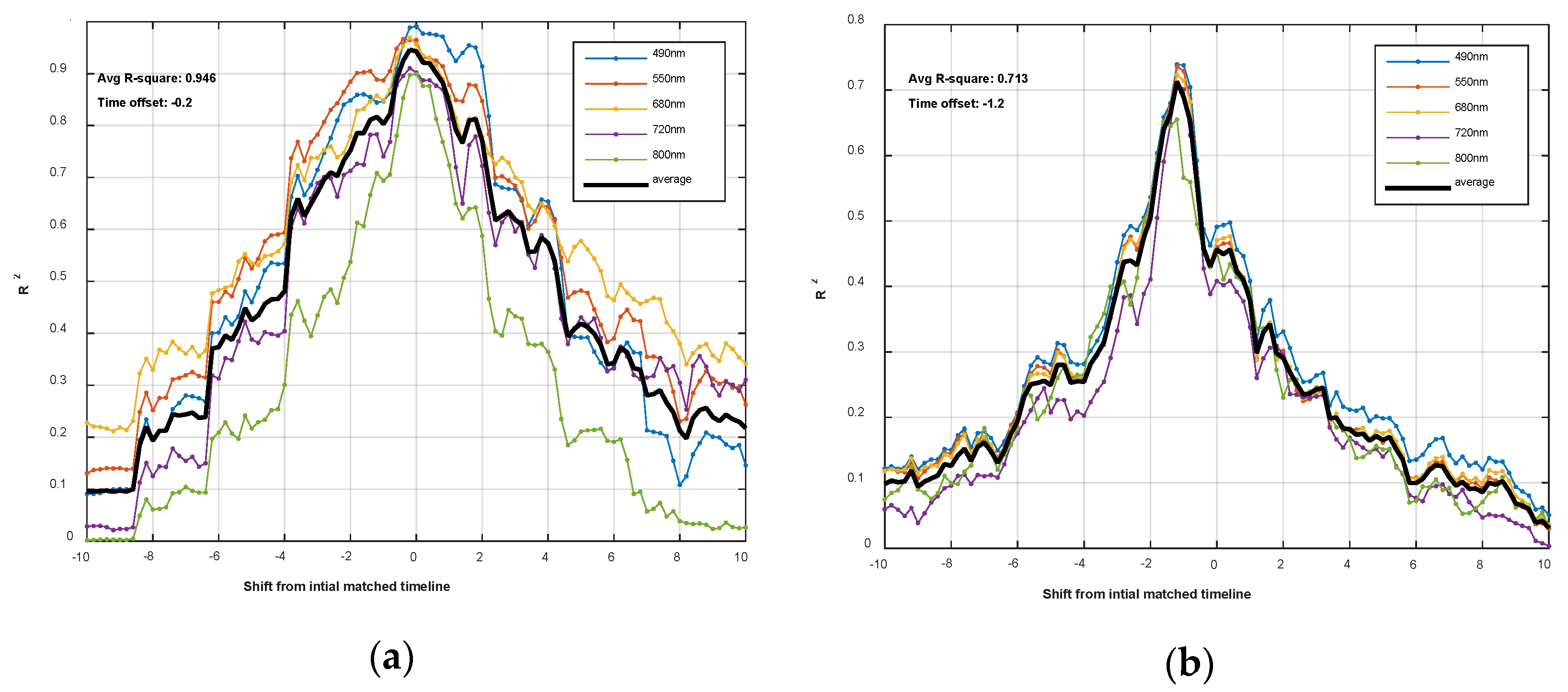
The profiles of R2 of multispectral–spectrometer data pairs at the ideal alignment (Δt = −0.2, Δx = 45, Δy = 5) at Site 1, and (Δt = −1.2, Δx = 85, Δy = −20) at Site 2, along the time domain, are given in Figure 4.
According to Figure 4, the best correlation for both sites was obtained for small time shifts of 1.2 s or less from their initial timeline match based on the nominal time tags; the time shift was not constant between the two sites because the sensors were reset or restarted before each flight. Furthermore, in cases where sensors have inaccurate clocks (more common for low-cost sensors), or they stay offline for a long time, their clocks may diverge from real world time, thereby rendering time alignment critical.
Either the individual bands, or their average at both sites, provides a clear unimodal R2 distribution over the time offset range. Site 2 has a lower R2 compared with Site 1, but still exhibits an obvious peak value. An explanation for the lower Site 2 correlations is that it had a larger population and more cover types (soybean, corn, soil, etc.), compared with Site 1. An analysis using a subset of samples in Site 1 (start, end, and the entirety of the flight) also reveals a similar trend, where lower sample numbers produced higher R2.
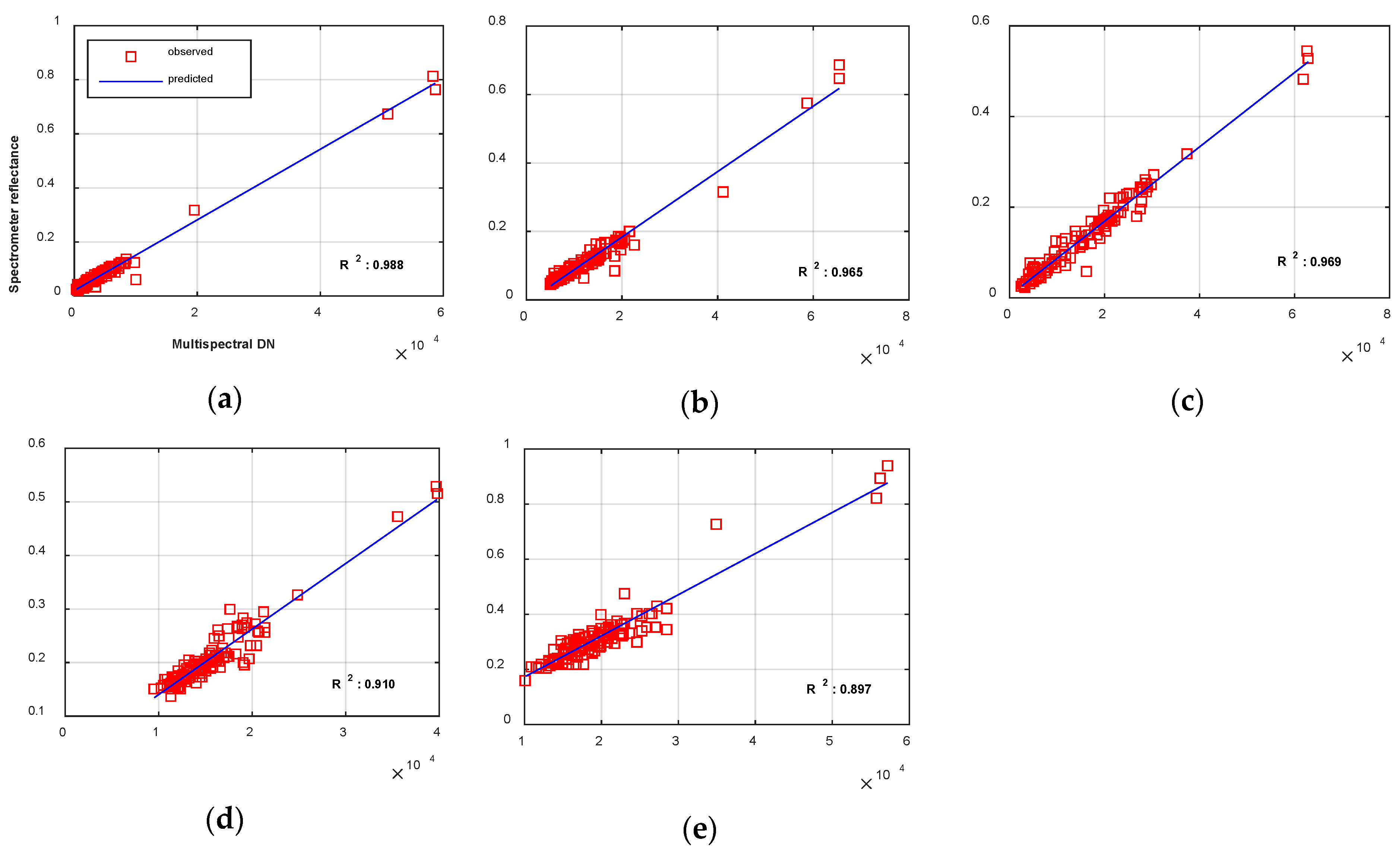
The correlation scatterplot for each spectral band with samples from the entire Site 1 flight at −0.2 s time offset, is provided in Figure 5. The distribution of samples in each band is quite similar, with R2 values ranging from 0.90 to 0.99.
4.1.2. Profile of Spatial Domain Alignment
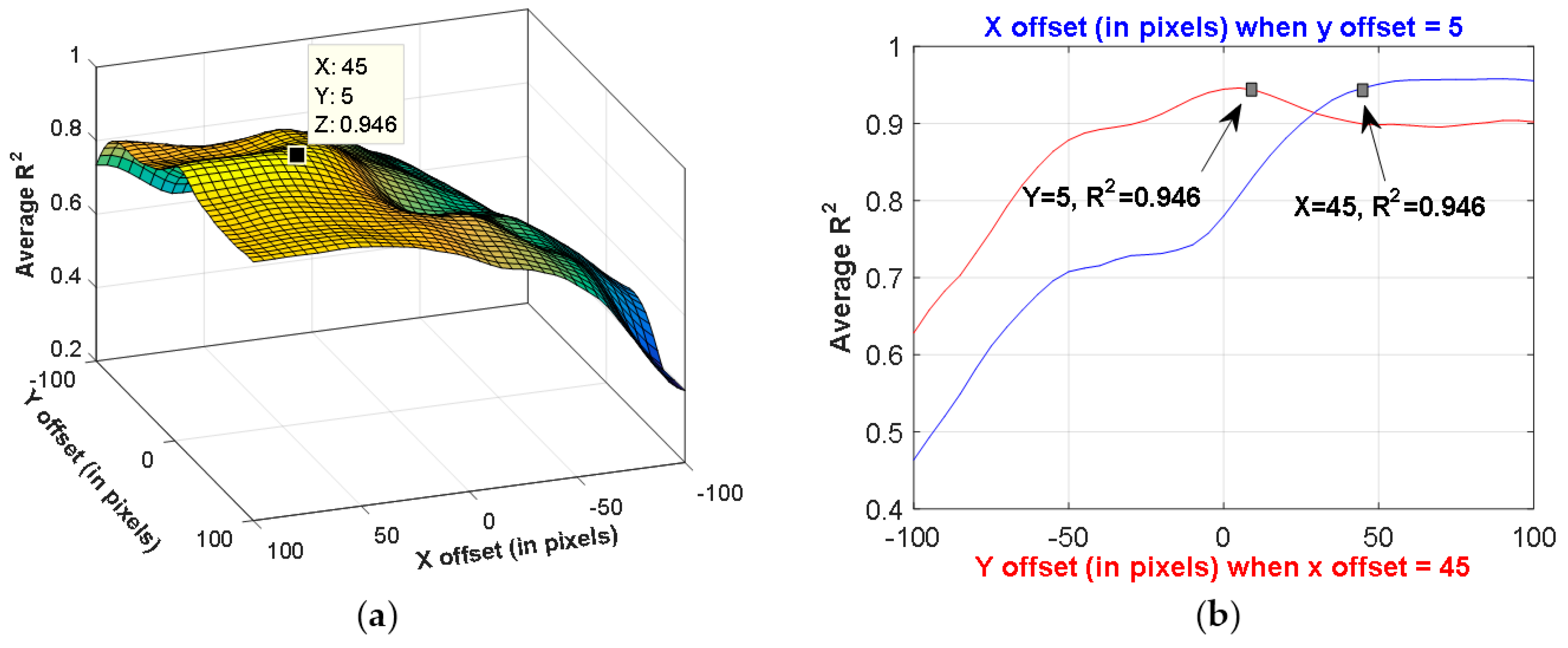
The profile of R2 distribution along the spatial domain at the ideal time offset (−0.2 s) in Site 1, is shown in Figure 6a, and the profiles over the X and Y directions are given in Figure 6b. A peak R2 value that was closest to the multispectral image center was selected; the resulting offset was Δx = +45, Δy = +5 pixels with R2 = 0.946 as shown in Figure 6a.
For Site 1, since the spectrometer footprint in the multispectral images for Site 1 was a circle with diameter of 48 pixels, a Y offset of 5 pixels is minor, especially considering the search interval was 5 pixels. This almost negligible offset probably resulted from fixing the spectrometer against the camera housing; rotational misalignment in the Y direction more than this small amount was not possible. In the X (flight) direction, however, the spectrometer was mounted by visually aligning the fiber optic cable and head with the vertically oriented edges of the camera body. The resulting 45 pixel offset in the X direction is not unexpected, and almost the same length as the footprint diameter. This spatial offset corresponds to 1.4° angular difference in the X direction between the multispectral camera and the spectrometer. Furthermore, Figure 6b shows an obvious R2 peak in the Y direction, but a plateau in R2 in the X direction. A possible explanation is that the flight lines (X direction) were parallel to rows of tomato plants in the site, causing R2 to be unchanged for certain offsets as both sensors detected radiance from the same row(s), but with a slight offset.
After data alignment in Site 1, an optimized parameter set, (Δt = −0.2, Δθ = 1.4°) or (Δt = −0.2, Δx = 45, Δy = 5) was obtained, with R2 of 0.946 between the multispectral camera image brightness and convoluted spectrometer reflectance. A similar trend of smaller Y offset was also found for the Site 2 data (Δx = 85, Δy = −20). Results from both sites show the need for the time and spatial domain alignment procedure. The resulting well-aligned data from the two sensors were then combined in the fusion procedure, as described in the next section.
4.1.3. Global Optimization vs. Two-Step Optimization
The global optimization of both time and space domain simultaneously involves intensive computation. To evaluate time and space offsets separately, the multi-hyperspectral data alignment was also optimized in a two-step process with the time domain processed first followed by the spatial domain. The alternative two-step optimization procedure starts by presuming that the spectrometer and camera are perfectly aligned first as shown in Equation (8).
After the alignment in the time domain where an optimized time offset is retrieved, the second step is alignment in the spatial domain, where () is optimized, as described in Equation (9), to obtain the best spatial shift (). Together with the optimized time offset retrieved in the first step, the alignment in both time and spatial domains is achieved via a combination of ().
This alternative two-step optimization was implemented and compared using the 128 spectrometer/image data samples of Site 1. The two-step optimization approach first reached = −0.2 s in the time domain and then () = (45, 5), which is the same alignment solution as the global optimization. The computation time using both approaches is reported as in Table 1.
The results were generated using a laptop with Intel CoreTM i7-5600U CPU @2.60 GHz, 12 GB RAM, and SSD drive, running a Windows 7 Professional 64-bit operation system. As in Table 1, the pre-processing stage used a large amount of time, because the convoluted multispectral band average values according to Equation (4) were calculated at each possible (Δx, Δy) in the spatial search range. The global optimization consumed 16.9 min while the two step-approach used 16.5 s; i.e., the two-step approach was about 60 times faster than the global optimization. The two-step optimization reported R2 = 0.81 for the first step (time-domain optimization) and then R2 = 0.95 for the second step, which equals that for the global optimization. Finally, a hyperspectral image (556 by 506 pixels after resampling) was generated using the data fusion approach in 8.5 min.
4.2. The Performance of Multispectral-Spectrometer Data Fusion
4.2.1. Accuracy of Data Fusion
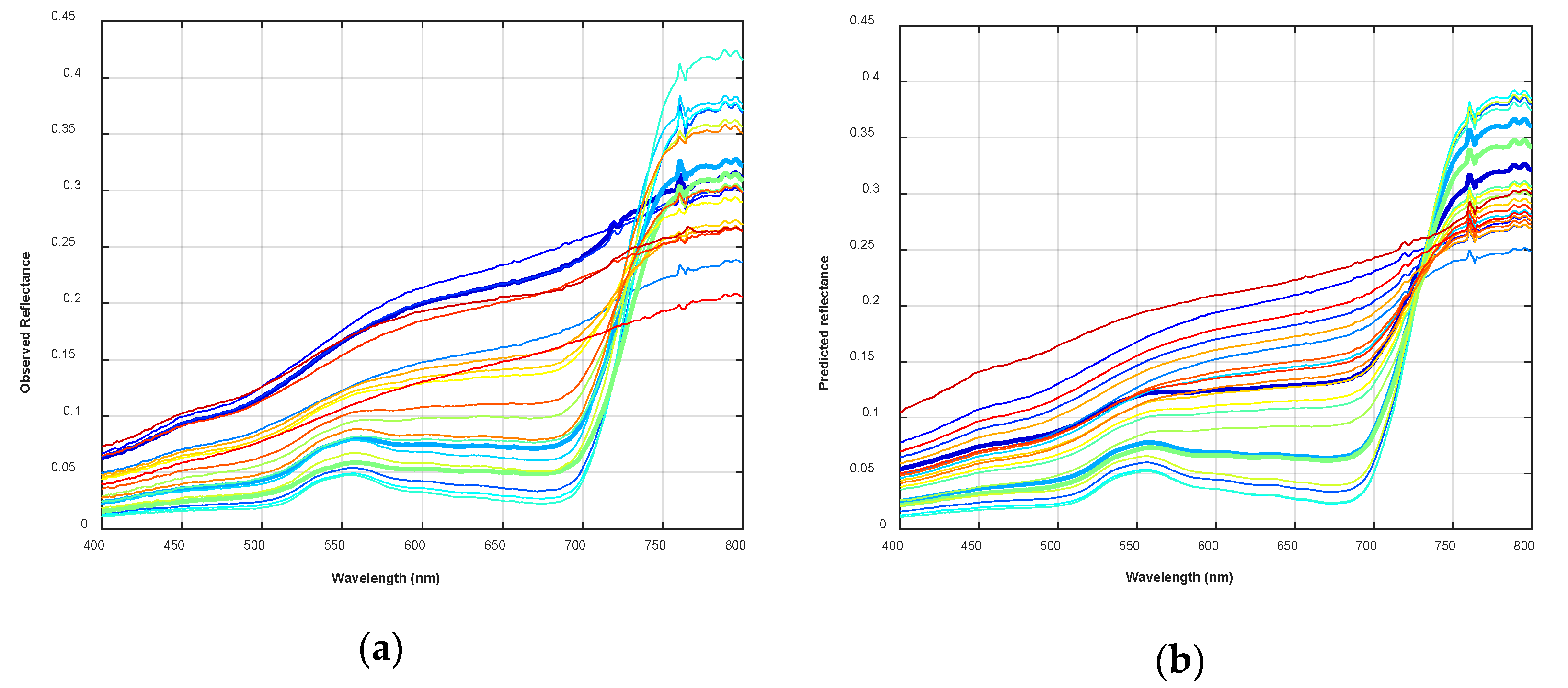
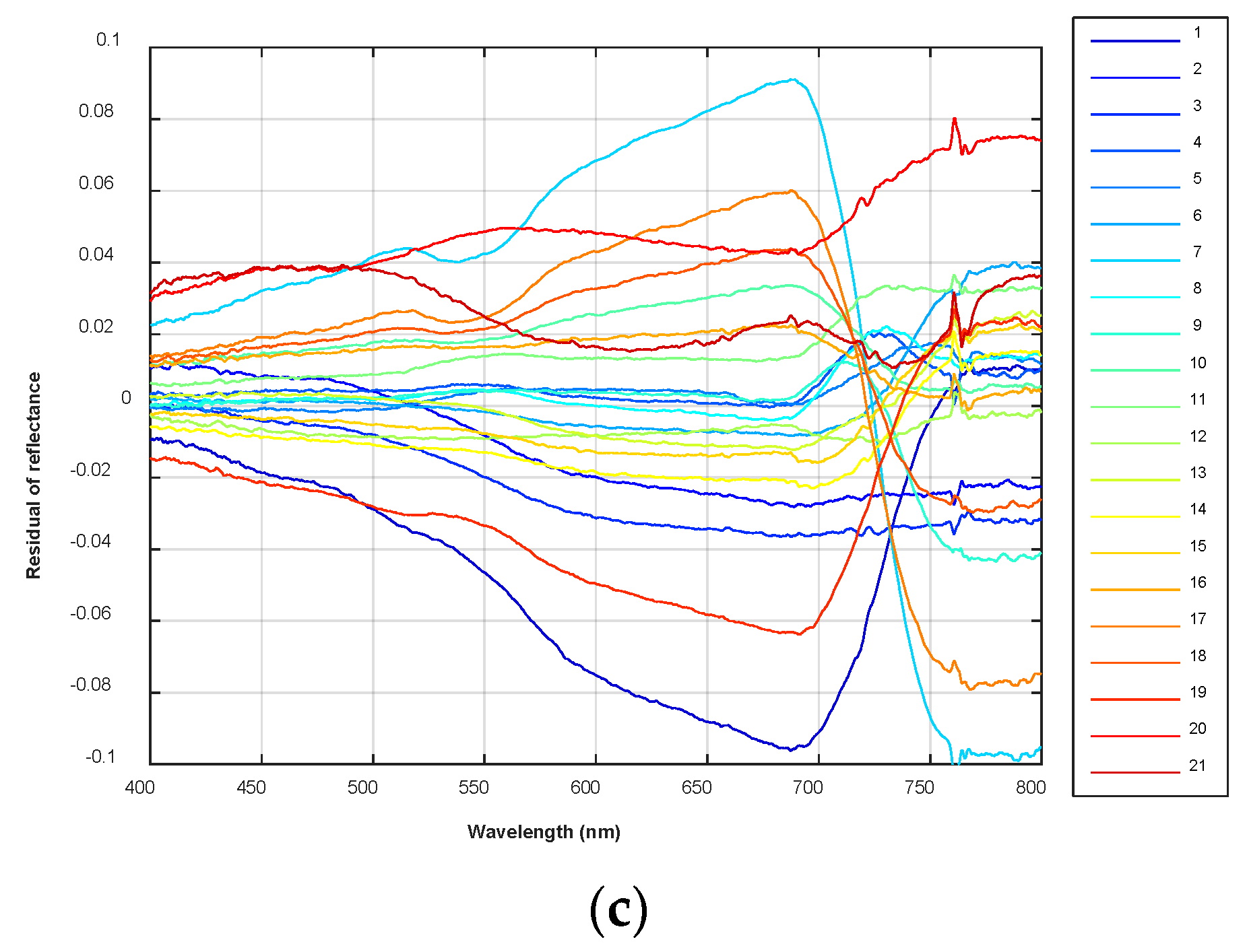
To predict full spectra at locations with only multispectral data, the PCA modelling method was implemented according to Equations (6) and (7), where m = 5 multispectral camera bands and n = 840 spectrometer bands within the wavelength range of 400 nm to 800 nm. The l = 128 samples of spectrometer and multispectral camera data taken from the optimal image location as determined in the previous section, were used as reference data in Equation (7). For validation purposes, 21 random samples of the spectrometer reflectance measurements were set aside, to be compared with predicted spectra. Thus k = 107 training data samples were used in the PCA imputation. Following experimentation with similar PCA methods [27,28,29], trimmed scores regression, based on the PCA method, was adopted in this study, because of its balance between prediction quality and robustness with data structure complexity and computation time [29]. The first three principal components were used in this procedure. According to suggested default values given in [28], the maximum number of iterations was set at 10, and the convergence tolerance was set at 0.0001. The 21 validation (observed) spectra, the corresponding predicted spectra, and the difference between them are shown in Figure 7a–c, respectively.
In Figure 7, the 21 validation spectra include vegetation (crops), soil, and some combined soil–vegetation data. The predicted curves in b have similar shapes and reflectance ranges, when compared with the observation curves in a. The absolute values of the “predicted–observed” residuals shown in c are all less than 0.1. The mean error, as a percentage of the residuals to the corresponding observations for the 21 validation samples is 9.48%, while the mean absolute error is 19.9%. According to Figure 7c, peak residuals usually occur around 680–700 nm, where reflectance of vegetation and soil has large contrast.
4.2.2. Stability of Data Fusion Parameters
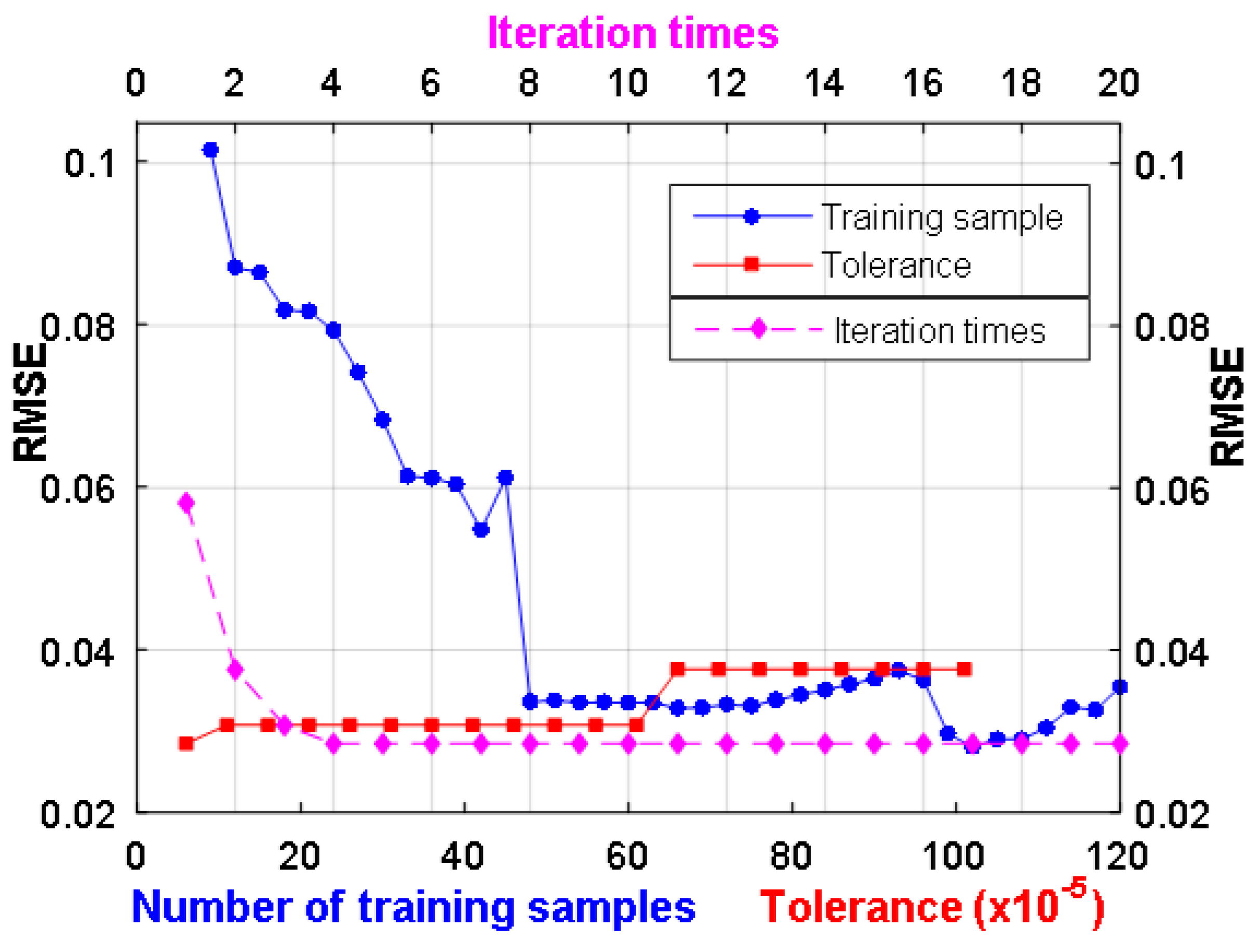
In addition, to test the impact of data fusion method parameters on accuracy, using Site 1 data, the data fusion step was run many times with each parameter changed as a sequence, and the corresponding RMSE of estimated hyperspectral spectra was computed. Specifically, the two PCA-based data fusion parameters were tested: iteration times (5–120, default 10), convergence tolerance (10−5–10−3, default 10−4), and the training sample number was also changed from 10, to 120. Figure 8 shows the impact of variations in converge tolerance on RMSE to be minor, while for RMSE was stable for numbers of iterations above 20. The number of training samples significantly affected RMSE; RMSE dropped after about 50 training samples among the 128 samples tested with the Site 1 data.
4.2.3. Comparison of Data Fusion Methods
To quantitatively compare the different data fusion methods described in Section 2.3, general accuracy evaluation measures, together with ones specifically designed for hyperspectral imagery, were used. In the results presented below, “ME” is the percent Mean Error, (predicted spectra–observed spectra)/observed spectra; “MAE” is the percent Mean Absolute Error; “RMSE” is the Root Mean Square of Error; and “STD_AE” is the Standard Deviation of the percent Absolute Error. For measures used in hyperspectral image quality evaluation [31,32], “SNR” is the signal to noise ratio; “UIQI” is the universal image quality index; “SAM” is spectral angle mapper; “ERGAS” is the relative dimensionless global error in synthesis, which calculates the amount of spectral distortion in the image; and “DD” is the degree of distortion. With the exception of SNR and UIQI, smaller values are better for all measures.
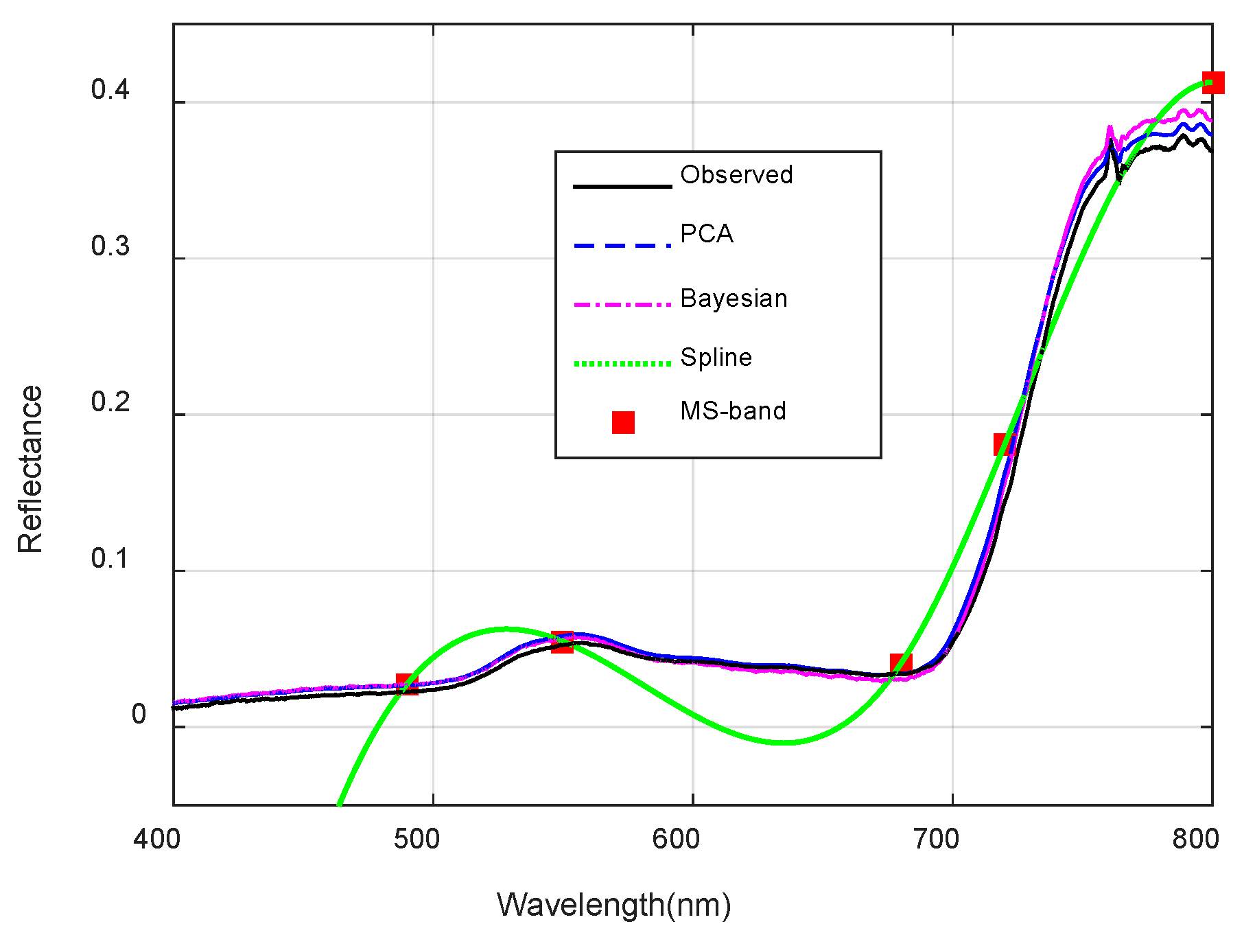
According to Table 2, PCA-based and Bayesian-based data fusion approaches performed similarly, especially the PCA group of methods. The Bayesian imputation with Gibbs sampling reported with the best overall performance, and used a slightly longer time than most other approaches. The spline approach was the simplest, and produced the worst predicted spectra accuracy. An example of a single crop location, estimated using the three fusion methods, Figure 9, illustrates the difference between these approaches. When comparing the data fusion result of the two study sites reported in Table 3, the PCA-based and Bayesian methods performed most consistently. For example, both of them produced MAE of around 17%, which means the absolute difference from predicted hyperspectral curves to the observed curves are around 17%. The ME is ±3% relative to the observed average in both sites in Table 3.
4.3. Fused Hyperspectral Imagery
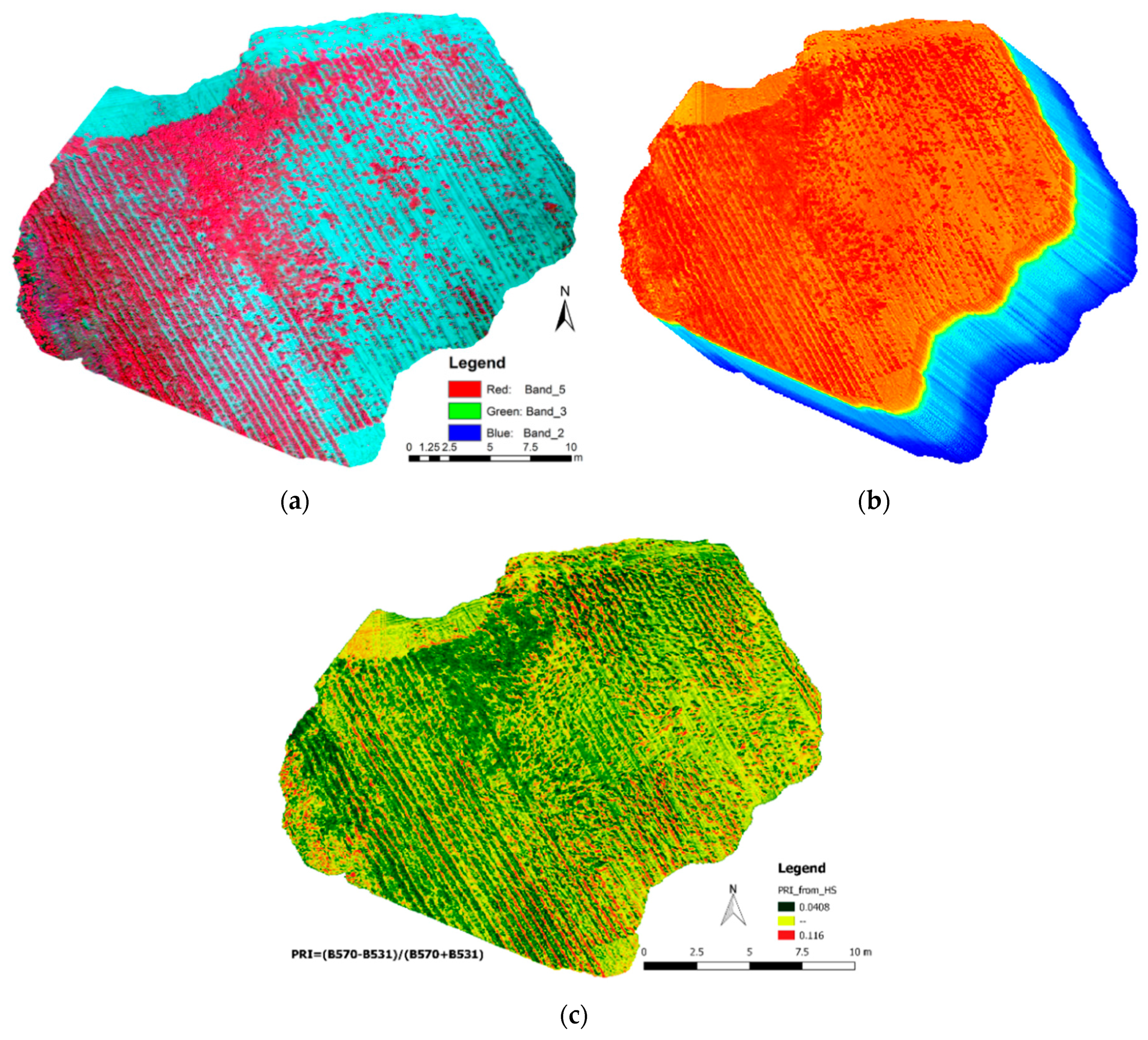
Once this approach to predict the hyperspectral reflectance was developed and evaluated, a subset of the multispectral camera images was mosaicked, and then used as input for hyperspectral image prediction. Agisoft Photoscan was employed to mosaic the multispectral images. The UAV on-board GPS/IMU provided the initial positions of each image center to assist the mosaicking process. Images for each spectral band, which had been calibrated using a Teflon surface, were then combined into a single TIFF file for input to the mosaicking procedure. The red band (680 nm) was set as the master band during mosaicking, as the multispectral camera sensitivity was highest in this region. The images were geocoded using the WGS84 + EGM96 Geoid coordinate system. The mosaic production process was automated; tie points were selected by the software. The default mosaicking approach of the software divides data into several frequency domains, which were then blended independently, with the blending effect decreasing with increasing distance from the seamline. The average control point position error was 1.99 m after bundle adjustment. The resulting false color mosaic, the generated hyperspectral image as an image cube, and a vegetation health index map are given in Figure 10, covering the area shown by the white polygon in Figure 3.
A hyperspectral image was then estimated from the multispectral mosaic using the fusion imputation methods described in Equations (6) and (7). To demonstrate the utility and advantage of such a hyperspectral image, a narrow band index, the Photo-chemical Reflectance Index (PRI) [33] was calculated as: (R570 − R531)/(R570 + R531), where R is reflectance extracted from the estimated hyperspectral imagery. The resulting PRI map is shown in Figure 9c. Red indicates low photosynthetic light use, while green indicates dense vegetation and high light use efficiency. Such an index cannot be calculated from multispectral camera data unless specific very narrowband interference filters are mounted on individual cameras. Such an approach would require changing filters if other indices incorporating different spectral bands were to be derived. In contrast, the estimated hyperspectral images allow derivation of a variety of such index maps from a single multispectral camera and spectrometer data set.
5. Discussion
The spectrometer footprint was assumed to be consistent in size and shape among samples, which is not always true. The UAV platform orientation fluctuated by wind and its own rotation. When the platform was tilted, the spectrometer footprint was an ellipsoid rather than a circle, as in the nadir case. Furthermore, the integration time brought in a considerable footprint shift at full UAV speed. Taking this study as an example, the 0.2 s integration time was equal to 1 m shift at full speed of 5 m/s. Hence, the shape of the footprint under the full speed is not a stationary circle, but a moving circle dragged through 1 m distance. Furthermore, the UAV needs to frequently accelerate and decelerate from one waypoint to another, accumulating the effect of tilt, velocity, and acceleration on the irregular shape of footprints. Despite including these sources of uncertainty, the proposed data alignment method handled the uncertainty quite well, mainly because the platform inclination consistently affects both hyperspectral and multispectral sensors, and the spatial auto-correlation with neighboring areas was carried through the observed data, and mitigated the effect of dragged footprint shapes.
The sources of uncertainty in the data fusion stage were numerous. A major source of uncertainty in the estimated spectra was the number of training samples, where many samples of convolved reflectance corresponded to a very similar multispectral band intensity combination, or vice versa. Figure 5 demonstrated such a trend in a linear regression model. Such an ambiguity of multispectral-hyperspectral sample pairing undermined the effectiveness of multi-hyperspectral data fusion method. Spectral mixing in the spectrometer footprint also complicates the imputation. Spectra prediction was poorer for pixels absent from the training set.
The broader impact of this study is significant. Drone and sensor technology are developing rapidly, with many manufacturers, standards, and products. There are compatibility issues among various sensors and platforms, due to differences in external computers, ports, triggering methods, and data storage methods. It is therefore challenging to operate sensors on a lightweight UAV using a single central control system, and impractical for general users (e.g., farmers) without advanced hardware and software skills. Accordingly, it is valuable that data from various sensors can be aligned post-flight by exploiting the correlations between two or more data types, as proposed in this study. Such a post-flight alignment approach allows farmers to use their existing equipment together with new sensors and platform, without advanced skills.
The proposed system has the advantage of very low cost and simple sensor positional/orientation control and measurement requirements compared to current hyperspectral cameras. It is a software solution that is easy to implement compared to development of a full UAV-based hyperspectral system. Consequently, it is well suited to precision farming applications on individual or small farms by farmers or other users with little remote sensing system expertise or funding. Results of this study can benefit precision farming companies, such as A&L Canada (http://www.alcanada.com/), which collaborated on this research, to offer services to the agriculture industry and farm owners. The system developed and evaluated in this study is expected to enhance capabilities to generate the high resolution information on crop condition and other environmental parameters needed in precision farming, water, and land use management.
6. Conclusions
This study demonstrated that a multispectral camera coupled with a spectrometer on a UAV platform can provide a means to estimate high spatial resolution hyperspectral imagery at very low cost for precision farming applications. The study involved two processes: alignment of data acquired by the two sensors, and fusion of the aligned data from the two sensors to estimate hyperspectral reflectance at all image pixel locations. In the sensor alignment process, as an alternative to more expensive and complex hyperspectral cameras, and as an alternative to complex positional and orientation measurement and processing, the multispectral camera and spectrometer were simply visually aligned in the UAV mount. A software approach was then used to align the datasets by determining the location in the image that corresponded to the spectrometer footprint collected closest to the image center. This data alignment procedure included analysis of correlations between the two data types for samples representing different acquisition timing between the two sensors and data offsets, due to sensor misalignment. The best location match for the spectrometer data was taken as the image pixels that maximized the correlation between the two data types. Empirical testing was conducted using UAV data acquired at 30 m altitude over a tomato farm and 50 m over a soybean/corn field with a mix of soil, vegetation and other land cover types. In a global optimization, a maximum R2 value of 0.95 was found at a −0.2 s time offset and an offset of 5 and 45 pixels in the X and Y directions, respectively, for one test site and −1.2 s, 85 and −20 pixels (X, Y) for the other site. A simplified two-step alignment approached was also tested which reaches the same alignment solution, but 60 times faster.
To fuse the multispectral camera and spectrometer data and produce a hyperspectral image, reflectance measured by the spectrometer was convolved to match the wider multispectral camera bands, and the pixel intensity values in the multispectral images were spatially averaged to match with spectrometer footprint. Three groups of spectra estimation methods were implemented; PCA-based and Bayesian-based estimation reported similar levels of residuals with mean absolute differences around 17% relative to the mean of observed spectra, and RMSE around 0.028 for the predicted spectra. A simple spline interpolation using the multispectral camera data proved to be ineffective in hyperspectral estimation. The tolerance and number of iterations had limited impact on the PCA-based data fusion method, which suggests the fusion method is stable. However, training sample numbers did have an effect; half of the 128 samples were required in training to maintain a stable low RMSE. The results reported for the two different flights over different crop types show consistent accuracy of predicted spectra. Using these results, a mosaic of multispectral images for a subarea was produced and used to predict the corresponding hyperspectral reflectance data at each pixel. The hyperspectral data were then used, as a demonstration, to map of narrowband PRI index, which is not possible using multispectral data unless the required narrowband filters (e.g., ±2 nm) are installed on individual cameras.
Acknowledgments
This project was funded by an NSERC Engage grant and NSERC Discovery funding. The authors are very grateful for the contributions of A&L Canada Laboratories in all phases of this research. We are grateful to the anonymous reviewers who contributed to the improvement of this manuscript.
Author Contributions
Chuiqing Zeng was responsible for the research design, field work plans, UAV flight campaign, data processing, experiments and manuscript drafting. Douglas J. King and Murray Richardson provided guidance and suggestions in the research design and provided important comments to shape this study in further stages. Douglas J. King also largely rewrote and polished the manuscript. Bo Shan carried out most field measurements and organized the equipment and personnel.
Conflicts of Interest
The authors declare no conflict of interest.
References
- Zhang, M.; Qin, Z.; Liu, X.; Ustin, S.L. Detection of stress in tomatoes induced by late blight disease in California, USA, using hyperspectral remote sensing. Int. J. Appl. Earth Obs. Geoinf. 2003, 4, 295–310. [Google Scholar] [CrossRef]
- Goel, P.K.; Prasher, S.O.; Landry, J.A.; Patel, R.M.; Viau, A.A.; Miller, J.R. Estimation of crop biophysical parameters through airborne and field hyperspectral remote sensing. Trans. Am. Soc. Agric. Eng. 2003, 46, 1235–1246. [Google Scholar]
- Lee, W.S.; Alchanatis, V.; Yang, C.; Hirafuji, M.; Moshou, D.; Li, C. Sensing technologies for precision specialty crop production. Comput. Electron. Agric. 2010, 74, 2–33. [Google Scholar] [CrossRef]
- Houborg, R.; Fisher, J.B.; Skidmore, A.K. Advances in remote sensing of vegetation function and traits. Int. J. Appl. Earth Obs. Geoinf. 2015, 43, 1–6. [Google Scholar] [CrossRef]
- Navarro-Cerrillo, R.M.; Trujillo, J.; de la Orden, M.S.; Hernández-Clemente, R. Hyperspectral and multispectral satellite sensors for mapping chlorophyll content in a mediterranean Pinus sylvestris L. Plantation. Int. J. Appl. Earth Obs. Geoinf. 2014, 26, 88–96. [Google Scholar] [CrossRef]
- Calderón, R.; Navas-Cortés, J.A.; Lucena, C.; Zarco-Tejada, P.J. High-resolution airborne hyperspectral and thermal imagery for early detection of verticillium wilt of olive using fluorescence, temperature and narrow-band spectral indices. Remote Sens. Environ. 2013, 139, 231–245. [Google Scholar] [CrossRef]
- Zarco-Tejada, P.J.; Catalina, A.; González, M.R.; Martín, P. Relationships between net photosynthesis and steady-state chlorophyll fluorescence retrieved from airborne hyperspectral imagery. Remote Sens. Environ. 2013, 136, 247–258. [Google Scholar] [CrossRef]
- Gevaert, C.M.; Suomalainen, J.; Tang, J.; Kooistra, L. Generation of spectral—Temporal response surfaces by combining multispectral satellite and hyperspectral uav imagery for precision agriculture applications. IEEE J. Sel. Top. Appl. Earth Obs. Remote Sens. 2015, 8, 3140–3146. [Google Scholar] [CrossRef]
- Roelofsen, H.D.; van Bodegom, P.M.; Kooistra, L.; van Amerongen, J.J.; Witte, J.-P.M. An evaluation of remote sensing derived soil pH and average spring groundwater table for ecological assessments. Int. J. Appl. Earth Obs. Geoinf. 2015, 43, 149–159. [Google Scholar] [CrossRef]
- Zarco-Tejada, P.J.; González-Dugo, M.V.; Fereres, E. Seasonal stability of chlorophyll fluorescence quantified from airborne hyperspectral imagery as an indicator of net photosynthesis in the context of precision agriculture. Remote Sens. Environ. 2016, 179, 89–103. [Google Scholar] [CrossRef]
- Candiago, S.; Remondino, F.; De Giglio, M.; Dubbini, M.; Gattelli, M. Evaluating multispectral images and vegetation indices for precision farming applications from uav images. Remote Sens. 2015, 7, 4026–4047. [Google Scholar] [CrossRef]
- Pajares, G. Overview and current status of remote sensing applications based on unmanned aerial vehicles (uavs). Photogramm. Eng. Remote Sens. 2015, 81, 281–329. [Google Scholar] [CrossRef]
- Jaakkola, A.; Hyyppä, J.; Kukko, A.; Yu, X.; Kaartinen, H.; Lehtomäki, M.; Lin, Y. A low-cost multi-sensoral mobile mapping system and its feasibility for tree measurements. ISPRS J. Photogramm. Remote Sens. 2010, 65, 514–522. [Google Scholar] [CrossRef]
- Suomalainen, J.; Anders, N.; Iqbal, S.; Roerink, G.; Franke, J.; Wenting, P.; Hünniger, D.; Bartholomeus, H.; Becker, R.; Kooistra, L. A lightweight hyperspectral mapping system and photogrammetric processing chain for unmanned aerial vehicles. Remote Sens. 2014, 6, 11013–11030. [Google Scholar] [CrossRef]
- Uto, K.; Seki, H.; Saito, G.; Kosugi, Y.; Komatsu, T. Development of a low-cost, lightweight hyperspectral imaging system based on a polygon mirror and compact spectrometers. IEEE J. Sel. Top. Appl. Earth Obs. Remote Sens. 2016, 9, 861–875. [Google Scholar] [CrossRef]
- Burkart, A.; Cogliati, S.; Schickling, A.; Rascher, U. A novel uav-based ultra-light weight spectrometer for field spectroscopy. IEEE Sens. J. 2014, 14, 62–67. [Google Scholar] [CrossRef]
- Aasen, H.; Burkart, A.; Bolten, A.; Bareth, G. Generating 3d hyperspectral information with lightweight uav snapshot cameras for vegetation monitoring: From camera calibration to quality assurance. ISPRS J. Photogramm. Remote Sens. 2015, 108, 245–259. [Google Scholar] [CrossRef]
- Liu, Y.; Wang, T.; Ma, L.; Wang, N. Spectral calibration of hyperspectral data observed from a hyperspectrometer loaded on an unmanned aerial vehicle platform. IEEE J. Sel. Top. Appl. Earth Obs. Remote Sens. 2014, 7, 2630–2638. [Google Scholar]
- Hruska, R.; Mitchell, J.; Anderson, M.; Glenn, N.F. Radiometric and geometric analysis of hyperspectral imagery acquired from an unmanned aerial vehicle. Remote Sens. 2012, 4, 2736–2752. [Google Scholar] [CrossRef]
- Zeng, C.; Richardson, M.; King, D.J. The impacts of environmental variables on water reflectance measured using a lightweight unmanned aerial vehicle (UAV)-based spectrometer system. ISPRS J. Photogramm. Remote Sens. 2017, 130, 217–230. [Google Scholar] [CrossRef]
- Rau, J.Y.; Jhan, J.P.; Huang, C.Y. Ortho-Rectification of Narrow Band Multi-Spectral Imagery Assisted by Dslr Rgb Imagery Acquired by a Fixed-Wing Uas. Int. Arch. Photogramm. Remote Sens. Spat. Inf. Sci. 2015, 40, 67–74. [Google Scholar] [CrossRef]
- Yahyanejad, S.; Rinner, B. A fast and mobile system for registration of low-altitude visual and thermal aerial images using multiple small-scale uavs. ISPRS J. Photogramm. Remote Sens. 2015, 104, 189–202. [Google Scholar] [CrossRef]
- Mobley, C.D. Light and Water: Radiative Transfer in Natural Waters; Academic Press: San Diego, CA, USA, 1994. [Google Scholar]
- Andover, C. Standard Bandpass Optical Filter. Available online: https://www.andovercorp.com/products/bandpass-filters/standard/600-699nm/ (accessed on 1 June 2016).
- Mello, M.P.; Vieira, C.A.O.; Rudorff, B.F.T.; Aplin, P.; Santos, R.D.C.; Aguiar, D.A. Stars: A new method for multitemporal remote sensing. IEEE Trans. Geosci. Remote Sens. 2013, 51, 1897–1913. [Google Scholar] [CrossRef]
- Villa, G.; Moreno, J.; Calera, A.; Amorós-López, J.; Camps-Valls, G.; Domenech, E.; Garrido, J.; González-Matesanz, J.; Gómez-Chova, L.; Martínez, J.A.; et al. Spectro-temporal reflectance surfaces: A new conceptual framework for the integration of remote-sensing data from multiple different sensors. Int. J. Remote Sens. 2013, 34, 3699–3715. [Google Scholar] [CrossRef]
- Murphy, K. Machine Learning: A Probabilistic Perspective; The MIT Press: Cambridge, MA, USA, 2012; p. 1096. [Google Scholar]
- Folch-Fortuny, A.; Arteaga, F.; Ferrer, A. Missing data imputation toolbox for matlab. Chemom. Intell. Lab. Syst. 2016, 154, 93–100. [Google Scholar] [CrossRef]
- Folch-Fortuny, A.; Arteaga, F.; Ferrer, A. Pca model building with missing data: New proposals and a comparative study. Chemom. Intell. Lab. Syst. 2015, 146, 77–88. [Google Scholar] [CrossRef]
- Grung, B.; Manne, R. Missing values in principal component analysis. Chemom. Intell. Lab. Syst. 1998, 42, 125–139. [Google Scholar] [CrossRef]
- Wei, Q.; Bioucas-Dias, J.; Dobigeon, N.; Tourneret, J.Y. Hyperspectral and multispectral image fusion based on a sparse representation. IEEE Trans. Geosci. Remote Sens. 2015, 53, 3658–3668. [Google Scholar] [CrossRef]
- Yokoya, N.; Grohnfeldt, C.; Chanussot, J. Hyperspectral and multispectral data fusion: A comparative review. IEEE Geosci. Remote Sens. Mag. 2017, in press. [Google Scholar] [CrossRef]
- Gamon, J.A.; Peñuelas, J.; Field, C.B. A narrow-waveband spectral index that tracks diurnal changes in photosynthetic efficiency. Remote Sens. Environ. 1992, 41, 35–44. [Google Scholar] [CrossRef]
Figure 1.
Illustration of unmanned aerial vehicle (UAV) flight system and the concept of data fusion. “FOV” stands for field of view.
Figure 1.
Illustration of unmanned aerial vehicle (UAV) flight system and the concept of data fusion. “FOV” stands for field of view.

Figure 2.
Need for alignment of the multispectral camera and spectrometer data. Δx and Δy are the offsets between the spectrometer data closest to the center of a multispectral image and the pixels at the center of the image. The offsets are caused by timing differences between the two sensors and by misalignment of the sensors’ optical axes. The goal was to determine and correct for Δt, Δx, and Δy before performing fusion of the two data types.

Figure 3.
The study site with the planned flight path (a), and the actual flight path (b) draped over a Google Earth image, taken on a later date (3 September 2016). (Site 1 at bottom left: tomato field; Site 2 in upper right: corn and soybean fields).
Figure 3.
The study site with the planned flight path (a), and the actual flight path (b) draped over a Google Earth image, taken on a later date (3 September 2016). (Site 1 at bottom left: tomato field; Site 2 in upper right: corn and soybean fields).

Figure 4.
Linear correlation between sample pairs of multispectral camera intensity and spectrometer reflectance at Site 1 (a) and Site 2 (b). Each subfigure includes five curves representing the five multispectral bands, plus a thicker line representing the average R2. Each curve is the correlation for the given band at 0.2 s interval time offsets over the ±10 s range. The maximum average R2 and its corresponding time offset are given in the upper left of each graph.

Figure 5.
Per band multispectral camera-spectrometer regression for the optimal time alignment at Site 1 for spectral bands at 490 nm, 550 nm, 680 nm, 720 nm, and 800 nm (a–e), respectively. “DN” is digital number, the intensity units of the multispectral camera signal.
Figure 5.
Per band multispectral camera-spectrometer regression for the optimal time alignment at Site 1 for spectral bands at 490 nm, 550 nm, 680 nm, 720 nm, and 800 nm (a–e), respectively. “DN” is digital number, the intensity units of the multispectral camera signal.

Figure 6.
Site 1 data alignment. (a) The distribution of R2 between the multispectral camera image brightness and spectrometer reflectance for spatial domain offsets (Δx, Δy) up to ±100 pixels at time offset = −0.2 s. (b) the separate X (left) and Y (right) profiles through the optimal location.
Figure 6.
Site 1 data alignment. (a) The distribution of R2 between the multispectral camera image brightness and spectrometer reflectance for spatial domain offsets (Δx, Δy) up to ±100 pixels at time offset = −0.2 s. (b) the separate X (left) and Y (right) profiles through the optimal location.

Figure 7.
The observed (a) and predicted (b) reflectance spectra and the corresponding residuals (c). Each spectrum is given a random color.
Figure 7.
The observed (a) and predicted (b) reflectance spectra and the corresponding residuals (c). Each spectrum is given a random color.


Figure 8.
The impact of data fusion parameters on hyperspectral data fusion.

Figure 9.
An example of the three types of data fusion compared with an observed spectrum over a crop sample at Site 1. The “PCA” is the “PCA_TSR” approach, “trimmed scores regression” defined in Section 3.2; the “Bayesian” is the “Bayesian_Gibbs” (Bayesian method with Gibbs sampling [27]) as defined in Section 3.2. “MS bands” are the spline interpolated reflectances derived directly from the multispectral (MS) camera data.

Figure 10.
Data fusion and hyperspectral imagery generation. (a) A preview of the multispectral subarea mosaic in false color (RGB: 800 nm, 680 nm, 550 nm). (b) The estimated hyperspectral (HS) image cube. (c) An example application of the estimated hyperspectral imagery: mapping a narrowband vegetation index, the Photo-chemical Reflectance Index (PRI).


Table 1.
Computation time consumption in optimization strategies.
| Optimization Methods | Pre-Processing | Time Domain | Space Domain | Data Fusion * |
|---|---|---|---|---|
| Global | 24.3 min | 16.9 min | 8.5 min | |
| Two-step | 1.9 s | 14.6 s | ||
* Data fusion to generate hyperspectral (HS) image used the PCA_TSR method reported later in Table 2.
Table 2.
Detailed comparison of fusion approaches implemented on the Site 1 data (tomato field).
| Category | Method | Time (s) | ME | MAE | RMSE (10−3) | STD_AE | SNR | UIQI | SAM | ERGAS | DD (10−3) |
|---|---|---|---|---|---|---|---|---|---|---|---|
| TSR | 0.46 | 3.63% | 16.83% | 28.947 | 0.137 | 14.97 | 0.960 | 12.37 | 22.10 | 20.751 | |
| KDR | 0.50 | 5.09% | 17.54% | 28.954 | 0.141 | 14.97 | 0.961 | 12.47 | 22.22 | 20.896 | |
| PCA | PCR | 0.49 | 3.63% | 16.83% | 28.947 | 0.137 | 14.97 | 0.960 | 12.37 | 22.10 | 20.751 |
| KDR–PLS | 0.67 | 3.57% | 16.78% | 28.953 | 0.137 | 14.97 | 0.960 | 12.37 | 22.11 | 20.746 | |
| PMP | 0.50 | 3.63% | 16.83% | 28.947 | 0.137 | 14.97 | 0.960 | 12.37 | 22.10 | 20.751 | |
| IA | 0.19 | 3.63% | 16.83% | 28.947 | 0.137 | 14.97 | 0.960 | 12.37 | 22.10 | 20.751 | |
| NIPALS | 0.68 | 4.46% | 16.69% | 29.357 | 0.139 | 14.85 | 0.959 | 12.42 | 22.51 | 21.039 | |
| DA | 124.20 | 3.19% | 17.40% | 28.906 | 0.146 | 14.99 | 0.961 | 12.43 | 22.23 | 20.785 | |
| Bayesian | Gibbs | 38.67 | 2.80% | 17.41% | 28.620 | 0.142 | 15.07 | 0.962 | 12.30 | 22.02 | 20.649 |
| EM | 1.03 | 3.25% | 17.35% | 28.895 | 0.145 | 14.99 | 0.961 | 12.42 | 22.23 | 20.773 | |
| ICM | 0.20 | 3.70% | 17.28% | 28.910 | 0.144 | 14.99 | 0.961 | 12.43 | 22.23 | 20.769 | |
| Spline * | 0.004 | −4.28% | 116.63% | 39.437 | 28.990 | 13.29 | 0.923 | 14.18 | 26.71 | 30.678 |
* Metrics for the spline approach were calculated in the wavelength range that is valid for the multispectral image (490–800 nm) rather than the full 400–800 nm range. The accuracy metrics are defined in the text: “ME” is the percent Mean Error, (predicted spectra–observed spectra)/observed spectra; “MAE” is the percent Mean Absolute Error; “RMSE” is the Root Mean Square of Error; and “STD_AE” is the Standard Deviation of the percent Absolute Error, “SNR” is the signal to noise ratio; “UIQI” is the universal image quality index; “SAM” is spectral angle mapper; “ERGAS” is the relative dimensionless global error in synthesis, which calculates the amount of spectral distortion in the image; and “DD” is the degree of distortion [31,32]. Bold text indicates best performance in a column.
Table 3.
Evaluation of hyperspectral data and multispectral image fusion result over the two agriculture sites.
Table 3.
Evaluation of hyperspectral data and multispectral image fusion result over the two agriculture sites.
| Method | #Image | #Training | #Test | Time (Min) | AvgR2 | Δt (s) | Δx (Pixel) | Δy (Pixel) | |||
|---|---|---|---|---|---|---|---|---|---|---|---|
| Site 1 (tomato) | 128 | 107 | 21 | 40.23 | 0.946 | −0.2 | 45 | 5 | |||
| Site 2 (corn/soybean) | 228 | 185 | 43 | 41.25 | 0.715 | −1.2 | 85 | −20 | |||
| Time (s) | ME | MAE | RMSE (10−3) | STD_AE | SNR | UIQI | SAM | ERGAS | DD (10−3) | ||
| Site 1 | PCA_TSR | 0.46 | 3.63% | 16.83% | 28.947 | 0.137 | 14.97 | 0.9597 | 12.37 | 22.10 | 20.751 |
| Bys_Gibbs | 38.67 | 2.80% | 17.41% | 28.620 | 0.142 | 15.07 | 0.9617 | 12.30 | 22.02 | 20.649 | |
| Spline | 0.004 | −4.28% | 116.63% | 39.437 | 28.990 | 13.29 | 0.9230 | 14.18 | 26.71 | 30.678 | |
| Site 2 | PCA_TSR | 0.54 | −1.37% | 16.99% | 27.244 | 0.284 | 15.34 | 0.9651 | 13.65 | 21.01 | 15.903 |
| Bys_Gibbs | 91.07 | −3.10% | 16.80% | 27.488 | 0.309 | 15.26 | 0.9652 | 13.83 | 20.99 | 15.586 | |
| Spline | 0.05 | −4.32% | 111.52% | 38.474 | 43.272 | 13.37 | 0.9326 | 15.14 | 26.37 | 26.987 | |
Note: “Method” are data fusion methods listed in Table 2. “#Image/Training/Test” are the number of samples for all, training, and test purposes, respectively. “AvgR2” is the average R2 among all the multispectral bands. The optimal alignment, (Δt, Δx, Δy) given as seconds in the time domain and pixels in the space domain. “Time” is the computation time in seconds (s) or minutes (min). “PCA_TSR” approach is “trimmed scores regression” in the PCA group defined in Section 3.2; “Bys_Gibbs” is the Bayesian method with Gibbs sampling [27] as defined in Section 3.2.
© 2017 by the authors. Licensee MDPI, Basel, Switzerland. This article is an open access article distributed under the terms and conditions of the Creative Commons Attribution (CC BY) license (http://creativecommons.org/licenses/by/4.0/).
Share and Cite
MDPI and ACS Style
Zeng, C.; King, D.J.; Richardson, M.; Shan, B. Fusion of Multispectral Imagery and Spectrometer Data in UAV Remote Sensing. Remote Sens. 2017, 9, 696. https://doi.org/10.3390/rs9070696
AMA Style
Zeng C, King DJ, Richardson M, Shan B. Fusion of Multispectral Imagery and Spectrometer Data in UAV Remote Sensing. Remote Sensing. 2017; 9(7):696. https://doi.org/10.3390/rs9070696
Chicago/Turabian StyleZeng, Chuiqing, Douglas J. King, Murray Richardson, and Bo Shan. 2017. "Fusion of Multispectral Imagery and Spectrometer Data in UAV Remote Sensing" Remote Sensing 9, no. 7: 696. https://doi.org/10.3390/rs9070696
Note that from the first issue of 2016, this journal uses article numbers instead of page numbers. See further details here.