Assessment of Approximations in Aerosol Optical Properties and Vertical Distribution into FLEX Atmospherically-Corrected Surface Reflectance and Retrieved Sun-Induced Fluorescence

Abstract

Physically-based atmospheric correction of optical Earth Observation satellite data is used to accurately derive surface biogeophysical parameters free from the atmospheric influence. While water vapor or surface pressure can be univocally characterized, the compensation of aerosol radiometric effects relies on assumptions and parametric approximations of their properties. To determine the validity of these assumptions and approximations in the atmospheric correction of ESA’s FLEX/Sentinel-3 tandem mission, a systematic error analysis of simulated FLEX data within the O${}_2$ absorption bands was conducted. This paper presents the impact of key aerosol parameters in atmospherically-corrected FLEX surface reflectance and the subsequent Sun-Induced Fluorescence retrieval (SIF). We observed that: (1) a parametric characterization of aerosol scattering effects increases the accuracy of the atmospheric correction with respect to the commonly implemented discretization of aerosol optical properties by aerosol types and (2) the Ångström exponent and the aerosol vertical distribution have a residual influence in the atmospherically-corrected surface reflectance. In conclusion, a multi-parametric aerosol characterization is sufficient for the atmospheric correction of FLEX data (and SIF retrieval) within the mission requirements in nearly 85% (70%) of the cases with average aerosol load conditions. The future development of the FLEX atmospheric correction algorithm would therefore gain from a multi-parametric aerosol characterization based on the synergy of FLEX and Sentinel-3 data.

1. Introduction

Atmospheric correction of optical Earth observation data is one of the critical steps in the data processing chain of a satellite mission as it allows deriving surface biogeophysical parameters free from the atmospheric influence [1,2]. Generally, atmospheric correction methods can be classified in two main families [3,4]: (1) empirical and (2) physically-based inversion methods. Empirical methods are based on mathematical approximations of the atmospheric radiative transfer equation and the inversion of surface properties directly from sensor data through empirical assumptions [5,6]. Physically-based methods [7,8,9,10] typically comprise two main steps: (1) derivation of key atmospheric parameters and (2) decoupling of surface properties from atmospheric effects by inversion of a Radiative Transfer Model (RTM). While empirical methods have a lower computation burden than physically-based inversion methods, their accuracy is also generally lower [1,6]. Consequently, when it comes to missions that require an accurate determination of surface properties, then physically-based inversion methods are preferred.

Physically-based atmospheric correction methods either apply an image-based retrieval of key atmospheric parameters, particularly (1) water vapor, (2) surface pressure and (3) aerosol properties, or take those parameters from external reference data [11,12]. Water vapor and surface pressure can be univocally determined, e.g., through differential absorption techniques [13] or meteorological pressure fields [11] and digital elevation models. However, the complete characterization of aerosol optical properties (e.g., extinction, absorption and scattering) can only be determined by instruments that provide multi-angular, multi-spectral and polarimetric capabilities such as the Multi-viewing, Multi-channel, Multi-polarization Imager (3MI) on-board of MetOp-Second Generation [14]. In addition, retrieval of aerosol vertical distribution is limited to active optical instruments such as the Cloud-Aerosol Lidar and Infrared Pathfinder Satellite Observation (CALIPSO) mission [15]. Unfortunately, such capabilities are usually not implemented in most optical satellite missions and thus most atmospheric correction algorithms aim to compensate the net radiometric effects of aerosol properties. In practice, this means that atmospheric correction algorithms typically implement parametric approximations or assume default values for some key aerosol properties. For instance, this is the case for advanced atmospheric correction methods such as applied to MEdium Resolution Imaging Spectrometer (MERIS)/Advanced Along Track Scanning Radiometer (AATSR) [10] where only aerosol optical thickness (AOT) and aerosol type (from a discrete set of standard aerosol types, e.g., [16]) are derived from satellite data by comparison against RTM-simulated Top-of-Atmosphere (TOA) radiances.

The question now arises whether the use of parametric approximations and assumptions about default values are sufficient to describe the impact of aerosol properties at TOA radiance. While approximations are generally implemented in most physically-based atmospheric correction methods [7,8,9,10], some studies remark the importance of typically neglected aerosol properties such as absorption [17] and vertical distribution [18,19] in atmospheric correction and radiative forcing of aerosols. This question is particularly relevant for the atmospheric correction of instruments measuring radiance in deep absorption bands at a high spectral resolution.

The European Space Agency’s (ESA) Fluorescence Explorer (FLEX) mission aims to derive global maps of vegetation Sun-Induced Fluorescence (SIF) from measurements in the deep Oxygen absorption bands at 687 nm and 760 nm [20,21]. FLEX is equipped with the FLuORescence Imaging Spectrometer (FLORIS) [22] that will measure radiance within these O${}_2$ bands at a spectral sampling of 0.1 nm, a spectral resolution of 0.3 nm and a spatial resolution of 300 m. At TOA level, SIF signal is around two orders of magnitude lower than the surface reflected radiance and thus errors appearing in the atmospheric correction can be largely propagated to errors in the retrieved SIF. FLEX will therefore make use of the synergy with Sentinel-3 [23], acquiring data over the same target with 6–15 s time delay at 300 m spatial resolution, to accurately characterize the atmospheric state.

The main objective of this paper, therefore, is to study the accuracy of using parametric approximations to describe the net radiometric effects of aerosol properties through their impact in atmospherically-corrected FLORIS data (i.e., surface reflectance) and subsequent retrieved SIF. Based on modeled data, we quantified how the net radiometric effects caused by a variability of aerosol types and vertical distributions are compensated by approximations in (1) the spectral behavior of the aerosol extinction, (2) the phase function and (3) the single-scattering albedo. These insights will ultimately contribute to support progress in atmospheric correction algorithms for the FLEX/Sentinel-3 tandem mission, and to reduce errors in the retrieval of SIF.

The remainder of the presented work is organized as follows. Section 2 gives an overview of aerosol optical properties and their common parametric approximations. Section 3 presents the materials and methods, specifically a newly developed software tool used to compute multi-dimensional look-up tables based on the execution of atmospheric RTMs. Section 4 focuses on the comparison of two simulated datasets in order to study how the implemented parametric approximations compensate the net radiometric effect of complex aerosol optical properties within the O${}_2$ bands. The analysis is conducted at three levels: (1) in the atmospherically-corrected FLEX data, (2) in the derived key aerosol parameters and (3) in the subsequent SIF retrieval. Finally, we conclude our work with a discussion of the results and their implications into FLEX atmospheric correction algorithm.

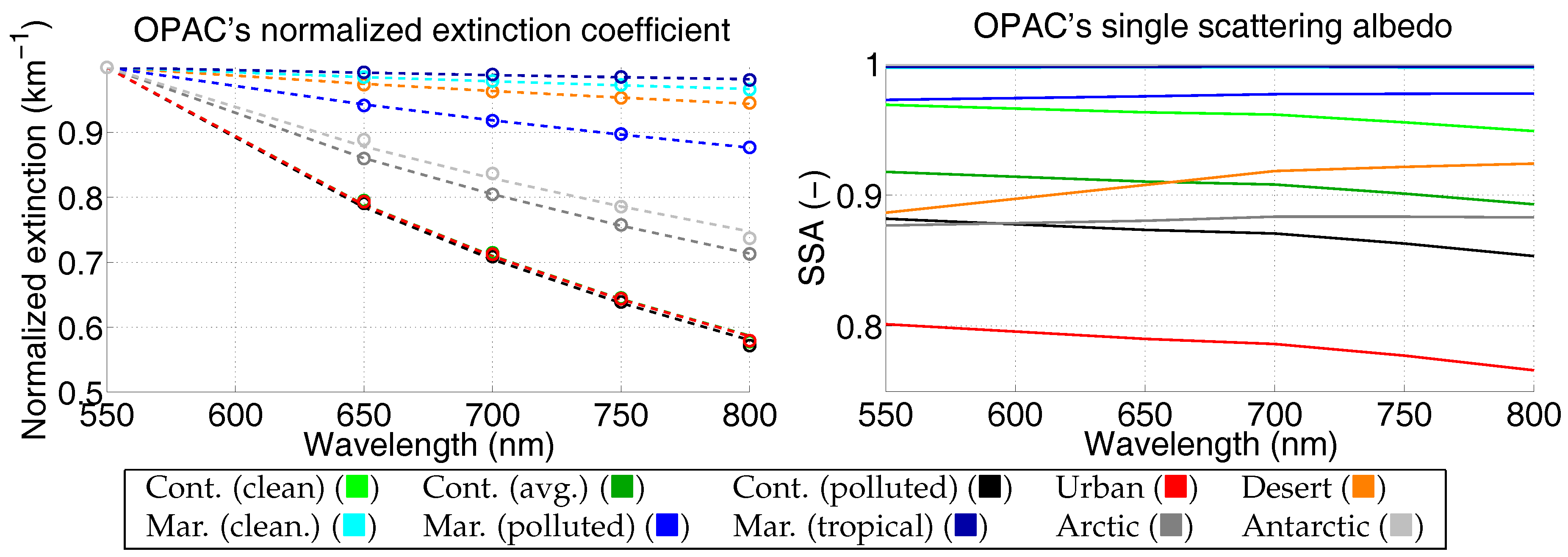
2. Aerosol Optical and Physical Properties

The propagation of an electromagnetic signal in some medium is described by its reflection, refraction, diffraction, absorption, polarization and scattering properties. In the Earth’s atmosphere, suspended matter (i.e., aerosol) is an important contributor to light absorption and scattering; specifically in the visible to short-wave infrared spectral range (from 400 nm to 2500 nm). With respect to their impact in light radiative transfer, aerosols can be described by their optical properties and their particle density vertical distribution in the atmosphere. Aerosol optical properties are typically characterized by their wavelength-dependent extinction coefficient ${\epsilon }_k$, which represents the loss of light per unit of optical path (usually in units of km${}^{-1}$). As shown in Equation (1), two mechanisms are sources of extinction: absorption (${\epsilon }_a$) and scattering (${\epsilon }_s$).

$${\epsilon }_k={\epsilon }_a+{\epsilon }_s$$

(1)

The proportion of scattering with respect the total extinction is represented by the wavelength-dependent single-scattering albedo (SSA), ${\omega }_0={\epsilon }_s/{\epsilon }_k$.

The amount and spectral behavior of the extinction coefficient is respectively driven by the number and proportion of small (0.1–2.5 $\mathsf{\mu }$m radius) and large (>2.5 $\mathsf{\mu }$m radius) particles, also known as fine and coarse modes. Each of these two modes can empirically be modeled by the Ångström law [24] in Equation (2):

$${\epsilon }_k(\lambda )={\epsilon }_k({\lambda }_0){\left(\frac{{\lambda }_0}{\lambda }\right)}^{\alpha }$$

(2)

where ${\lambda }_0$ is a reference wavelength and $\alpha$ is the so-called Ångström exponent, which is also wavelength-dependent [25].

Additionally, the angular distribution of the scattered light with respect to the incident beam depends on the aerosol’s particle shape and size. The aerosol phase function ${\mathrm{\Phi }}_{\lambda }(\theta ,\varphi )$ represents, for a given wavelength $\lambda$, the fraction of scattered light in the direction represented by the scattering and azimuth angles ($\theta$ and $\varphi$ respectively). Typically, azimuthal symmetry is assumed given the random orientation of aerosol particles. The aerosol phase function can be described by the wavelength-dependent asymmetry parameter $g_{\lambda }$, which is the average over all scattering directions of the cosine of the scattering angle as in Equation (3):

$$g_{\lambda }=2\pi {\int }_0^{\pi }{\mathrm{\Phi }}_{\lambda }(\theta )cos\theta sin\theta d\theta$$

(3)

Given this asymmetry parameter, the phase function can then be computed assuming a mathematical formulation such as the Mie theory for spherical particles [26] or the parametric Henyey-Greenstein (HG) approximation [27] (see Equation (4)).

$$\mathrm{\Phi }{(\theta )}_{HG}=\frac{1}{4\pi }\frac{1-g^2}{{(1+g^2-2gcos\theta )}^{3/2}}$$

(4)

With these aerosol optical properties (extinction, absorption and phase function), the effects of aerosols onto radiance detected by a sensor can be further described by considering the vertical distribution (i.e., height profile) of aerosol particle density. Aerosol particle density typically follows a decreasing vertical distribution with, in normal meteorological conditions, higher densities in the boundary layer (0 km to ∼2 km) and troposphere (∼2 km to 10 km) [16]. Among these two layers, variability and mixture of aerosol types is higher in the boundary region [28,29] due to interactions between land surface and atmosphere (e.g., biomass burning, dust storms or urban pollution). The vertical distribution in each layer largely depends on particle density and meteorological conditions, particularly wind, turbulence and vertical profiles of pressure and temperature. The variability of this vertical distribution can be partially calculated with numerical weather prediction models [30]. However, these models are neither practical for simulation of large databases nor for near-real time atmospheric correction algorithms. Instead, aerosol vertical distribution is typically modeled with simple empirical approximations such a decreasing exponential [16] (see Equation (5)):

$${\epsilon }_k(h)\sim exp(-h/Z)$$

(5)

Here, the extinction coefficient at an altitude h (in km), ${\epsilon }_k(h)$, is driven by the scale height parameter Z (in km). The integral of the extinction coefficient over the entire atmospheric column (0–100 km) is known as Aerosol Optical Thickness (AOT), which is also wavelength dependent.

3. Materials and Methods

To facilitate evaluating the impact of introduced approximations and assumptions on aerosol properties in the atmospheric correction of FLORIS TOA radiance and the subsequent SIF retrieval, we developed a new software tool (see Section 3.1) to simulate several surface reflectance datasets (see Section 3.2). The implemented method for the analysis and comparison of these datasets is further presented in Section 3.3.

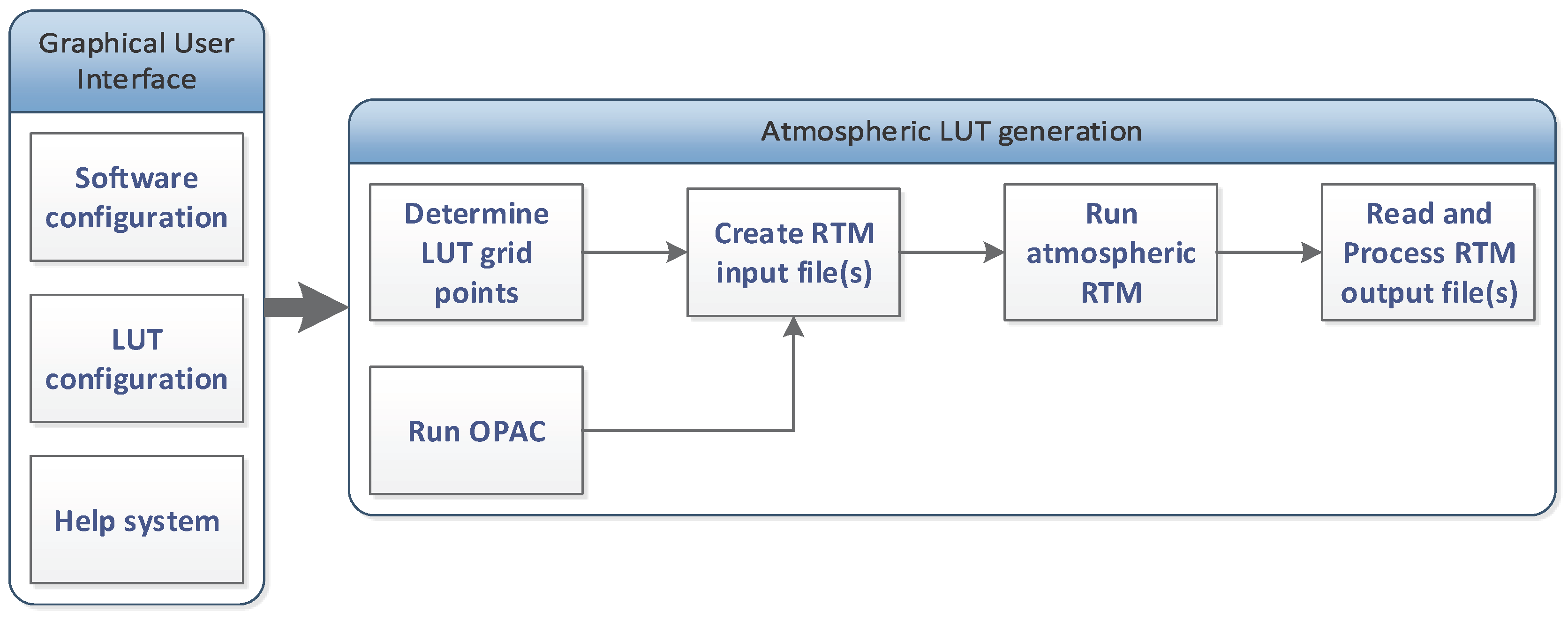
3.1. Atmospheric Look-Up Table Generator

With the purpose of automating the generation of the datasets used in this work, we developed a friendly graphical user interface software tool (Atmospheric Look-up table Generator: ALG, v1.0) that enables executing the MODerate resolution atmospheric TRANsmission (MODTRAN) RTM (v5.2.1) [31] (see Figure 1) and generates large multi-dimensional look-up tables. In addition, similarly to AEROgui [32], ALG integrates the Optical Properties of Aerosols and Clouds (OPAC) (v3.1) database [16]. When coupled with an atmospheric RTM, OPAC expands the pre-defined RTM aerosol models with a large and comprehensive database of complex aerosol optical properties.

ALG also allows users to (see Figure 2):

• Define input key atmospheric variables including among others: aerosol types (default and OPAC user-defined), aerosol vertical distribution in the boundary layer (model default or exponential function), phase function (Mie or HG), spectral dependency of aerosol extinction (model default or Ångström exponent), SSA (model default or spectrally constant).
• Define input geometric conditions such as viewing and illumination zenith/azimuth angles, surface height and sensor altitude.
• Set the spectral range and resolution of the output data at non-contiguous spectral intervals.

As shown in Figure 1, ALG first generates the RTM input files corresponding to: (1) all combinations of input key variables or (2) a near-random sampling of the input variable space based on the Latin Hypercube sampling (LHS) distribution [33]. Second, parallel instances of a RTM are run on a process similar to the implemented in [34]. Last, the output database is computed. It contains the following atmospheric transfer functions for each combination of key input parameters:

• Atmospheric path radiance ($L_0$)
• At-surface direct and diffuse solar irradiance ($E_{dir}$ and $E_{dif}$).
• Target-to-sensor direct and diffuse transmittance ($T_{dir}$ and $T_{dif}$).
• Spherical albedo (S).

The computation of the above atmospheric transfer functions is performed using the MODTRAN5 interrogation technique developed by Guanter et al. (2009) [35].

3.2. Description of Simulated Datasets

We used the ALG tool to produce three MODTRAN5-based datasets for the analysis of aerosol properties in the spectral range around the O${}_2$-B (680–700 nm) and O${}_2$-A (755–775 nm) bands. MODTRAN5 was chosen to generate these three datasets given that it accurately simulates the coupled effects of absorption and scattering through its correlated-k option [36].

The first dataset (further referred to as analysis) functions to evaluate the relative contribution into TOA radiance of various aerosol optical properties and vertical distribution thanks to the versatility in MODTRAN5 to introduce user-defined aerosol properties. Thus, this dataset (see

Table 1. Key input aerosol variables for the analysis dataset. This dataset consists of 2000 samples with a LHS distribution.

Variable Name	Min	Max
Ångström exponent ($\alpha$) (-):	0.05	2
HG parameter (g) (-):	0.6	1
AOT${}_{550}$ (-):	0.05	0.4
SSA (-):	0.85	1
Aerosol scale height (Z) (km):	2	99
Aerosol top height ($H_{max}$) (km):	1	3

) includes typical variability [12,16,17] in: (1) the AOT at 550 nm (AOT${}_{550}$); (2) the spectral dependency of the extinction coefficient, through the Ångström exponent; (3) the phase function, through the HG asymmetry parameter; (4) the single scattering albedo; and (5) the vertical distribution, through the scale height Z and top height of the boundary layer $H_{max}$. The analysis dataset consists of 2000 samples with a LHS distribution at a spectral resolution of 5 cm${}^{-1}$ (approx. 0.3 nm at 760 nm).

The second dataset (further referred to as reference) aims to reproduce a realistic set of FLORIS TOA radiances observations. The OPAC aerosol database is used to provide a realistic and varied set of wavelength-dependent aerosol optical properties (e.g., extinction, absorption and asymmetry parameter) in the boundary layer. Furthermore, this dataset varies the aerosol vertical distribution by considering several values of the aerosol scale height and top height in the boundary layer.

Table 2. Key input aerosol parameters for the reference dataset.

Variable Name	Values
Aerosol types (in the boundary layer):	MODTRAN: Rural, Maritime, Urban, Desert, Tropospheric. OPAC: Continental (clean, average, polluted), Urban, Desert, Maritime (clean, polluted, tropical), Arctic, Antarctic
AOT${}_{550}$ (-):	0.05, 0.12, 0.21, 0.3, 0.4
Aerosol scale height (Z) (km):	2, 3.5, 8, 15, 99
Aerosol top height ($H_{max}$) (km):	1, 1.5, 1.75, 2, 2.25, 2.5, 3

summarizes the values of the key aerosol variables for the reference dataset, with a total of N${}_{ref}$ = 2625 combinations.

The third dataset (further referred to as retrieval) implements parametric approximations and assumptions on the aerosol optical properties and vertical distribution. Therefore, the retrieval dataset aims to represent the data used in an atmospheric correction algorithm. We consider the following approximations and assumptions on the aerosol optical properties and vertical distribution:

• A single Ångström Law with spectrally-invariant Ångström exponent reproduces the effective spectral dependency of the extinction coefficient of both fine and coarse modes in the boundary layer and troposphere.
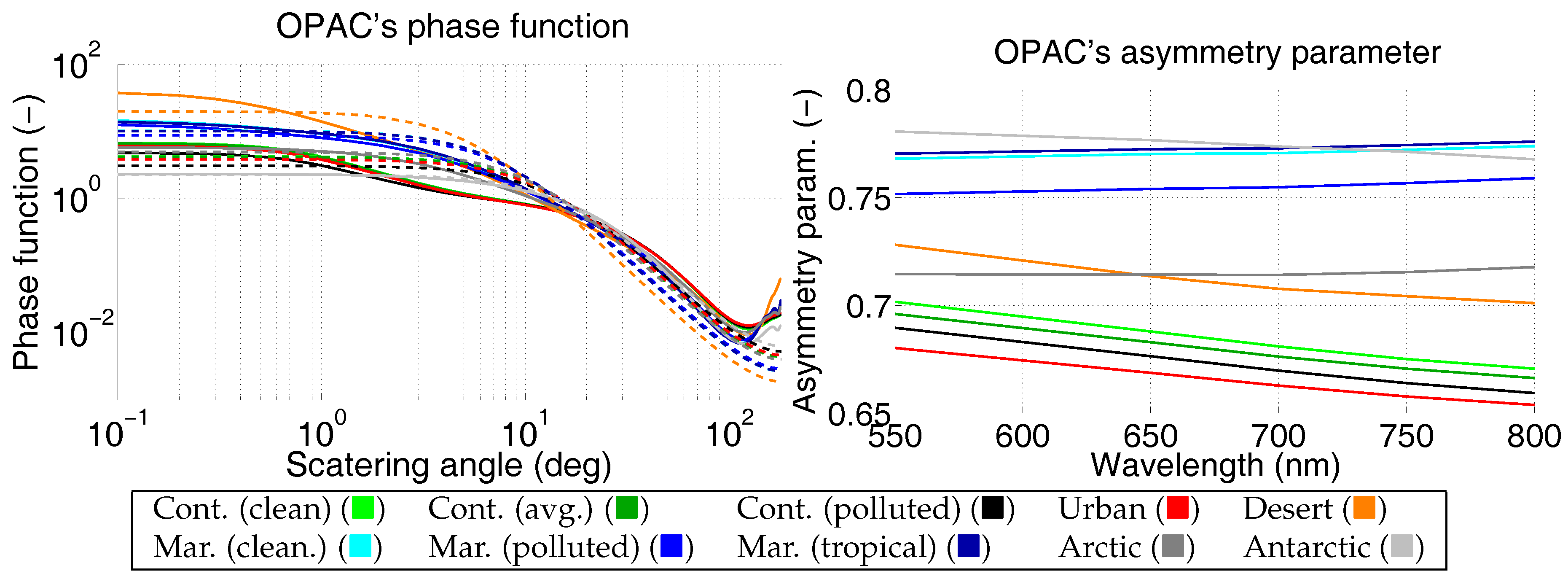
• The aerosol scattering phase function is modeled by the HG approximation with a spectrally-invariant asymmetry parameter.
• Different aerosol types have a low variability of values and spectral dependency of the SSA [17] and, therefore, it is considered to be spectrally-invariant in the 680–775 nm region.
• For spaceborne measurements, it is considered that the aerosol vertical distribution has a lower impact in TOA radiance than the caused by the variability of AOT${}_{550}$, Ångström exponent, asymmetry parameter and SSA. Thus, we assume that a predefined aerosol vertical distribution is representative of the net radiometric effect of most vertical distributions.

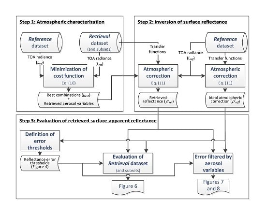
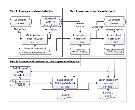
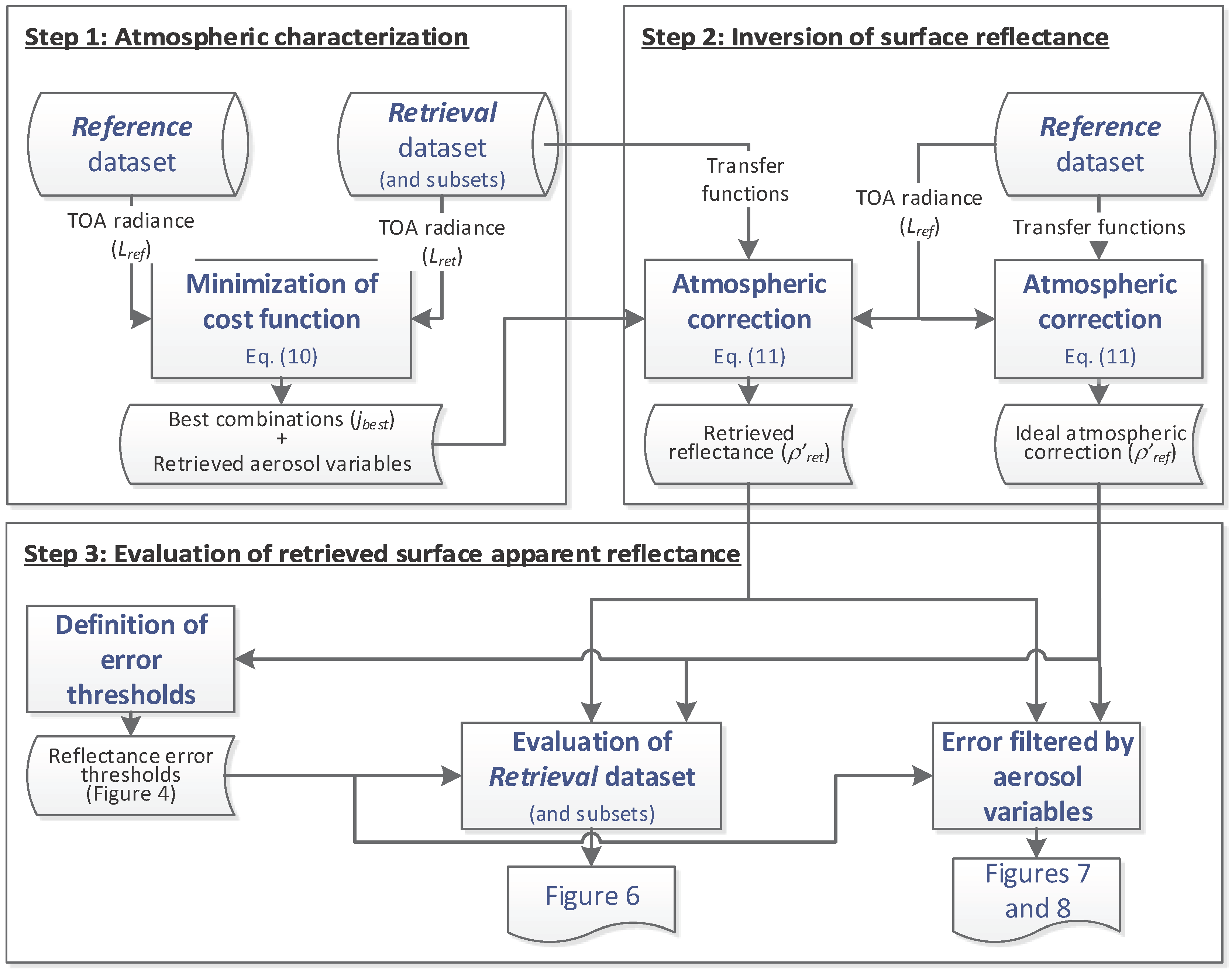
In order to sample the full key input parameter space, we used a LHS distribution with a total of N${}_{ret}$ = 3500 samples.

Table 3. Key input aerosol parameters for the retrieval dataset. This dataset consists of 3500 samples with a LHS distribution.

Variable Name	Min	Max
Ångström exponent ($\alpha$) (-):	0.05	2
HG parameter (g) (-):	0.6	1
AOT${}_{550}$ (-):	0.03	0.43
SSA (-):	0.75	1
Aerosol vertical distribution:	MODTRAN mid-latitude summer

summarizes the minimum/maximum values of each key aerosol variables for the retrieval dataset.

Further, in order to evaluate the impact of additional simplifications and assumptions, the retrieval dataset was divided into four subsets as shown in

Table 4. Fixed and ranging variables for each subset of the retrieval dataset.

Subset ID	Ranging Variables	Fixed Variables and Values	Comment
#1	AOT${}_{550}$	$\alpha$ (1 ± 0.2), g (0.82 ± 0.02), SSA (0.93 ± 0.015)	Represents a typical atmospheric correction strategy fixing the aerosol type
#2	AOT${}_{550}$, g, $\alpha$	SSA (0.93 ± 0.015)	Varying atmosphere with fixed SSA
#3	AOT${}_{550}$, g, SSA	$\alpha$ (1 ± 0.2)	Varying atmosphere with fixed spectral dependency of aerosol extinction
#4	AOT${}_{550}$, $\alpha$, SSA	g (0.82 ± 0.02)	Varying atmosphere with fixed phase function

:

Both the reference and the retrieval datasets were generated at high spectral resolution with a spectral sampling of 0.1 cm${}^{-1}$ (approx. 0.006 nm at 760 nm).

For each sample in the analysis, reference and retrieval datasets, we calculated the corresponding TOA radiance spectra by coupling the generated atmospheric transfer functions with a reference Lambertian surface reflectance ($\rho$) and isotropic SIF (F) spectra (see Figure 3) following Equation (6):

$$L=L_0+\frac{T(E_{tot}\rho +\pi F)}{\pi (1-S\rho )}$$

(6)

where T = T${}_{dir}$ + T${}_{dif}$ is the total target-to-sensor transmittance and E${}_{tot}$ = E${}_{dir}cos{\theta }_{il}$ + E${}_{dif}$ is the total at-surface irradiance for a solar zenith angle of ${\theta }_{il}$ (55${}^{\circ }$ in our case). The Lambertian surface reflectance assumption is considered to be valid due to the coarse resolution of the FLEX data (300 m) [9] and since the near-nadir observation geometry is not in hot spot direction [37,38].

We simulated synthetic FLORIS TOA radiance data for each sample of the reference and the retrieval datasets. The high spectral resolution TOA radiance from Equation (6) was resampled to a lower spectral resolution data to mimic FLORIS data. This was achieved through convolution with FLORIS spectral response function, modelled with a double error function (see Equation (7)):

$$f_{\lambda }=\frac{1}{2}\left[erf\left(\lambda ;s,c,b\right)-erf\left(\lambda ;s,c,-b\right)\right]$$

(7)

Here $erf(\lambda ;s,c\pm b)$ represents an error function (see Equation (8)) evaluated in the high resolution wavelength domain $\lambda$ at the spectral channel centered at the wavelength c:

$$erf(\lambda ;s,c,\pm b)=\frac{2}{\sqrt{\pi }}{\int }_0^{-s(\lambda -c\mp b/2)}exp(-t^2)dt$$

(8)

The parameters s = 17.5 and b = 0.3 nm represent respectively the slope of the error function and the full-width at half maximum of FLORIS spectral response function. The synthetic FLORIS TOA radiance, $\langle L\rangle$, was therefore obtained by the convolution in Equation (9) for a set of spectral channels c in the range around the O${}_2$-B and O${}_2$-A absorptions and with a spectral sampling of 0.1 nm.

$$\langle L\rangle =\frac{\int f_{\lambda }Ld\lambda }{\int f_{\lambda }d\lambda }$$

(9)

3.3. Data Analysis

In order to identify the aerosol properties in FLORIS data variables, we first conducted a global sensitivity analysis (GSA) of the TOA radiance simulations from the analysis dataset. GSA explores the full input variable space and evaluates the relative importance of each input variable in a model [39]. The method can be used to identify the most influential variables affecting model outputs. In variance-based GSA, the contribution of each input variable to the variation in outputs is averaged over the variation of all input variables, i.e., all input variables are changed together. In a related study [40,41], the method of Satelli et al. (2010) [42] was applied to the SCOPE model [43,44] to identify the driving variables that shape the variability of canopy-leaving SIF spectrum across its full spectral range. The method has been demonstrated to be effective in identifying both the main sensitivity effects (first-order effects, i.e., the contribution to the variance of the model output by each input variables) and total sensitivity effects (the first-order effects plus interactions with other input variables, $S_{Ti}$) of input variables. However, as many simulations are required, i.e., typically about 1000 per input variable, GSA is a computationally expensive method and thus limited by the processing speed of the model under study. In order to bypass the computational burden of costly RTMs, a computationally effective technique has recently been proposed by only using a limited number of RTM executions. The technique consists of approximating the RTM by a surrogate model with low computation time, also referred to as meta-model or emulator [45]. Once having a successful emulator developed, the idea is that it can replace the original RTM and be readily applied to perform sensitivity analysis. Accordingly, emulators can provide an efficient mean for applying a GSA to large and expensive models, including the computationally expensive MODTRAN model. An earlier study over the full 400–2500 nm MODTRAN spectral range confirms the applicability of the proposed method [46]. Here, we extended this method for the GSA of TOA radiance within the O${}_2$-B (680–700 nm) and O${}_2$-A (755–775 nm) bands at a spectral resolution of 5 cm${}^{-1}$ (approx. 0.3 nm at 760 nm). The residuals of the emulator used for GSA were first analyzed on their accuracy; the residuals are a factor ∼20 lower than variations in TOA radiance caused by errors of 1% in key input aerosol parameters, and can thus be considered as accurate for the GSA.

Secondly, we analyzed the impact of approximations in aerosol properties in FLORIS atmospherically-corrected surface reflectance. To do so, we applied the approach shown in the flow chart illustrated in Figure 4, and described in the following paragraphs.

The first step aims to reproduce the atmospheric characterization step of a physically-based atmospheric correction algorithm. This step consists on finding the sample ($j_{best}$) in the retrieval dataset that best matches each sample (i) in the reference dataset by minimizing the cost function in Equation (10) as proposed in [9,10]:

$$j_{best}=\underset{j}{min}e(i,j)=\underset{j}{min}\sqrt{\frac{1}{n}\sum _{c=1}^n{({\widehat{L}}_{ref}^i-{\widehat{L}}_{ret}^j)}^2},$$

(10)

where the subindex $ref$ and $ret$ refer respectively to the reference and the retrieval datasets. The cost function $e(i,j)$ only considers the n spectral channels, c, outside the O${}_2$ absorption bands.

The second step performs the atmospheric correction, inverting the apparent reflectance ($\overline{\rho }$) of each reference dataset spectra from the first order Taylor expansion of Equation (6) [20] (see Equation (11)).

$$\langle L_{ref}^i\rangle =\langle L_0\rangle +\frac{\langle T·E_{tot}\rangle \overline{\rho }}{\pi }+\frac{\langle T·E_{tot}·S\rangle {\overline{\rho }}^2}{\pi }$$

(11)

Here, the apparent reflectance ($\overline{\rho }$) couples the effect of surface emitted SIF and Sun-reflected radiance, i.e., E${}_{tot}\overline{\rho }$ = E${}_{tot}\rho$ + $\pi$ F. The brackets $\langle ·\rangle$ represent the result of convolving the high spectral resolution atmospheric transfer functions by FLORIS spectral response function following Equations (7)–(9).

The atmospheric correction is applied to the reference and retrieval datasets:

• In the reference dataset, the retrieved surface apparent reflectance ${\overline{\rho }}_{ref}$ corresponds to an ideal atmospheric correction algorithm from perfectly known atmospheric conditions.
• In the retrieval dataset, the retrieved surface apparent reflectance ${\overline{\rho }}_{ret}$ corresponds to the actual product of an atmospheric correction algorithm. The best matching combinations (j${}_{best}$) are taken from the estimated atmospheric conditions from the first step (i.e., atmospheric characterization). The apparent reflectance will be later used to retrieve SIF emission through spectral decomposition techniques ([47]).

In the third step, we evaluate the accuracy of the approximations in aerosol properties through the accuracy of the retrieved surface apparent reflectance. To do so, we compute the relative error between ${\overline{\rho }}_{ref}$ and ${\overline{\rho }}_{ret}$ and its average in each O${}_2$ absorption band (i.e., 686.6–699.5 nm for the O${}_2$-B and 759.3–767.5 nm for the O${}_2$-A). The relative error in surface apparent reflectance is compared against the threshold defined as the relative difference between ${\overline{\rho }}_{ref}$ and ${\overline{\rho }}_{ref+0.2}$ (see Figure 5). Here, ${\overline{\rho }}_{ref+0.2}$ results of an ideal atmospheric correction of a new dataset based on the key input atmospheric parameters in Table 2 and increasing F in Equation (6) by $\Delta F$ = 0.2 mW·m${}^{-2}·$sr${}^{-1}·$nm${}^{-1}$. This $\Delta F$ is the SIF threshold error as defined by FLEX mission requirements [21,48].

Two surface reflectance error assessment were performed to evaluate the accuracy of the atmospheric correction:

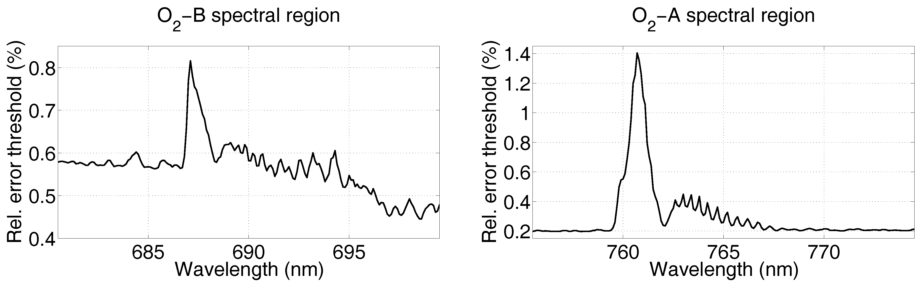
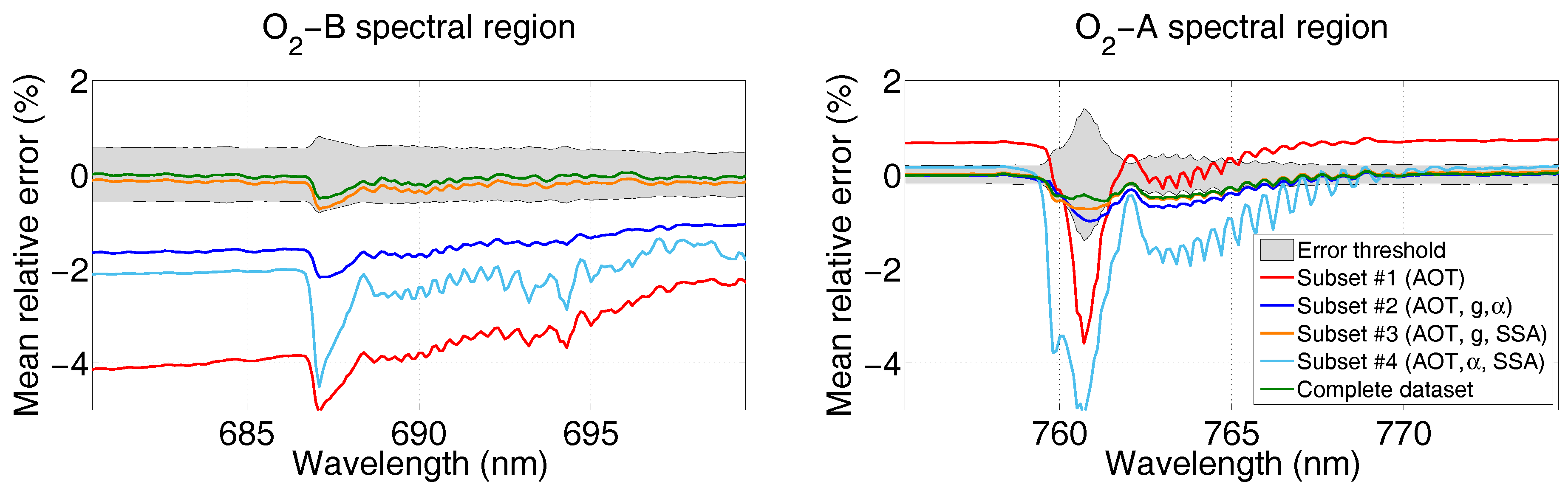
• We calculated the mean relative error, i.e., the average for all the samples in the reference dataset, after the atmospheric correction and compared it with the relative error threshold shown in Figure 5. This mean relative error is calculated for the surface apparent reflectance retrieved using the complete retrieval dataset and its four subsets (see Table 4). Through this analysis, we evaluated the overall impact of the various aerosol properties on the atmospheric correction.
• We filtered the relative error in apparent reflectance, averaged within each O${}_2$ absorption, as a function of the key input variables of the reference dataset. Through this analysis, we determined in more detail the source of errors in the atmospheric correction of the reference dataset using the complete retrieval dataset.

Thirdly, we analyzed the retrieved values (average and standard deviation) of the key aerosol variables against the reference values derived from OPAC aerosols in [16]. The reference values of Ångström exponent and HG asymmetry parameter were obtained from the best fitting of the extinction coefficient and the phase function (at 700 nm) respectively with the Ångström law and the HG phase function. The reference value of the SSA was calculated by averaging the SSA in the 650–800 nm spectral range.

Finally, we analyzed the impact of approximations in aerosol properties in the retrieved SIF after the atmospheric correction. For each retrieved apparent reflectance ${\overline{\rho }}_{ret}^i$ (i from 1 to N${}_{ref}$) and in each O${}_2$ region, SIF${}_{ret}^i$ was retrieved based on the Spectral Fitting Method described in [47]. We selected the wavelength range 686.7–688.3 nm for the O${}_2$-B and 757.3–765.5 nm for the O${}_2$-A. In order to analyze the error propagation from atmospheric correction to the retrieved SIF, and to minimize the errors associated with the Spectral Fitting Method, we assumed a known real reflectance and applied a linear polynomial for the retrieved SIF. For the complete reference dataset, we then computed the root-mean-square error between the reference and retrieved SIF, filtered by AOT${}_{550}$, and calculated the error statistic. The SIF error threshold was set to 0.2 mW·m${}^{-2}·$sr${}^{-1}·$nm${}^{-1}$ according to FLEX mission requirements [21,48].

4. Results

Following the method described in Section 3.3, we now show the results corresponding to: (1) the conducted GSA applied to FLORIS TOA radiance (Section 4.1), (2) the effect of approximated aerosol properties on the inversion of surface apparent reflectance (Section 4.2), (3) the accuracy of retrieved key aerosol optical properties (Section 4.3), and (4) the propagation of atmospheric correction errors on the retrieved SIF (Section 4.4).

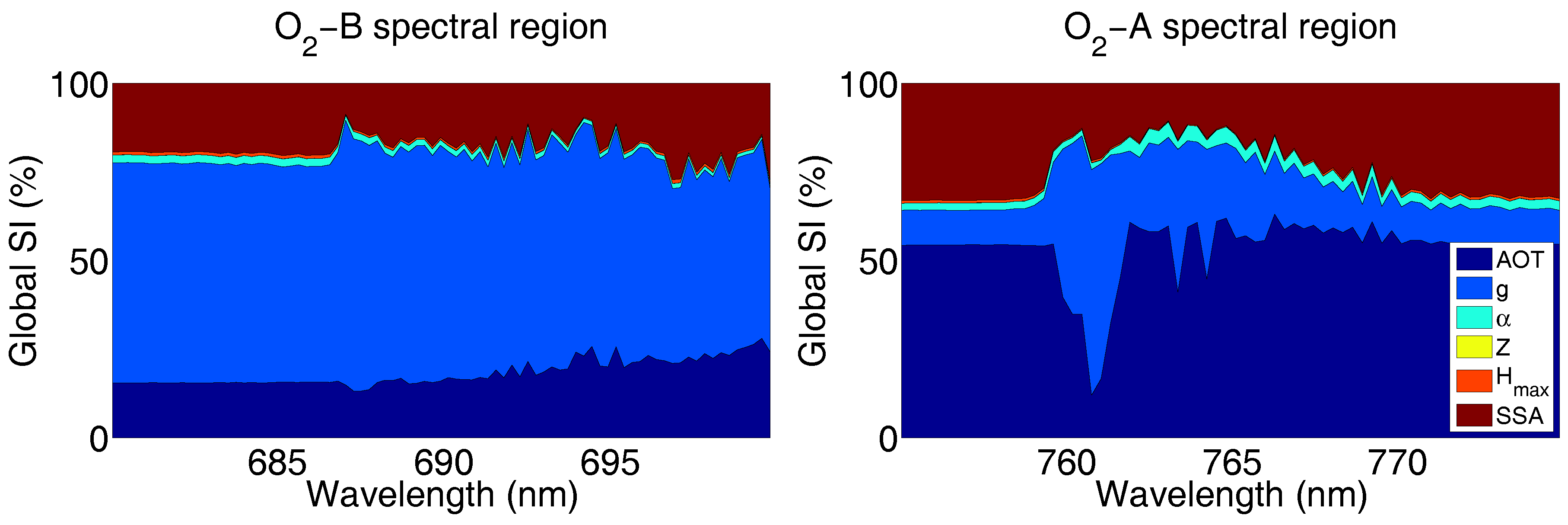
4.1. Relative Contribution of Aerosol Parameters in FLORIS TOA Radiance

The total sensitivity index ($S_{Ti}$) over the analysis dataset allows us studying the relative contribution of each aerosol variable, thus determining which of the key variables should be retrieved in an atmospheric correction algorithm for FLEX. Figure 6 shows this relative contribution evaluated by $S_{Ti}$ for each spectral channel in the O${}_2$-B (left) and O${}_2$-A (right). Each aerosol variable is represented with a different color: AOT${}_{550}$ in dark blue, HG asymmetry parameter (g) in blue, Ångström exponent ($\alpha$) in cyan, scale height (Z) in yellow, top height of the boundary layer ($H_{max}$) in orange and single scattering albedo (SSA) in dark red.

In general terms, it can be noted that TOA radiance is mainly driven by atmospheric variables related to scattering processes (i.e., the HG asymmetry parameter (G), the SSA and the AOT${}_{550}$) but some points must be outlined:

• The non-isotropy of the aerosol phase function (evaluated through the HG asymmetry parameter) has indeed the largest contribution (50–60%) in the TOA radiance. Particularly, since aerosol scattering is higher at shorter wavelengths, the contribution of the aerosol phase function is higher in all spectral channels within the O${}_2$-B and at the bottom of the O${}_2$-A band (∼761 nm).
• The AOT${}_{550}$ is the second driving variable, particularly outside the O${}_2$-A absorption band and on the secondary absorptions (762–770 nm).
• The remaining sensitivity is dominated by the SSA with an influence of 20% in the O${}_2$-B and 40% in the O${}_2$-A spectral regions outside the absorption bands. The influence of the SSA is reduced to 10–20% inside the absorption bands.
• The spectral dependency of the extinction coefficient (evaluated through the Ångström exponent) has lower impact than AOT${}_{550}$, SSA and g in both O${}_2$ regions, particularly inside the O${}_2$-B absorption band.
• The aerosol vertical distribution, evaluated through the Z and $H_{max}$ parameters, has a residual influence on the TOA radiance.

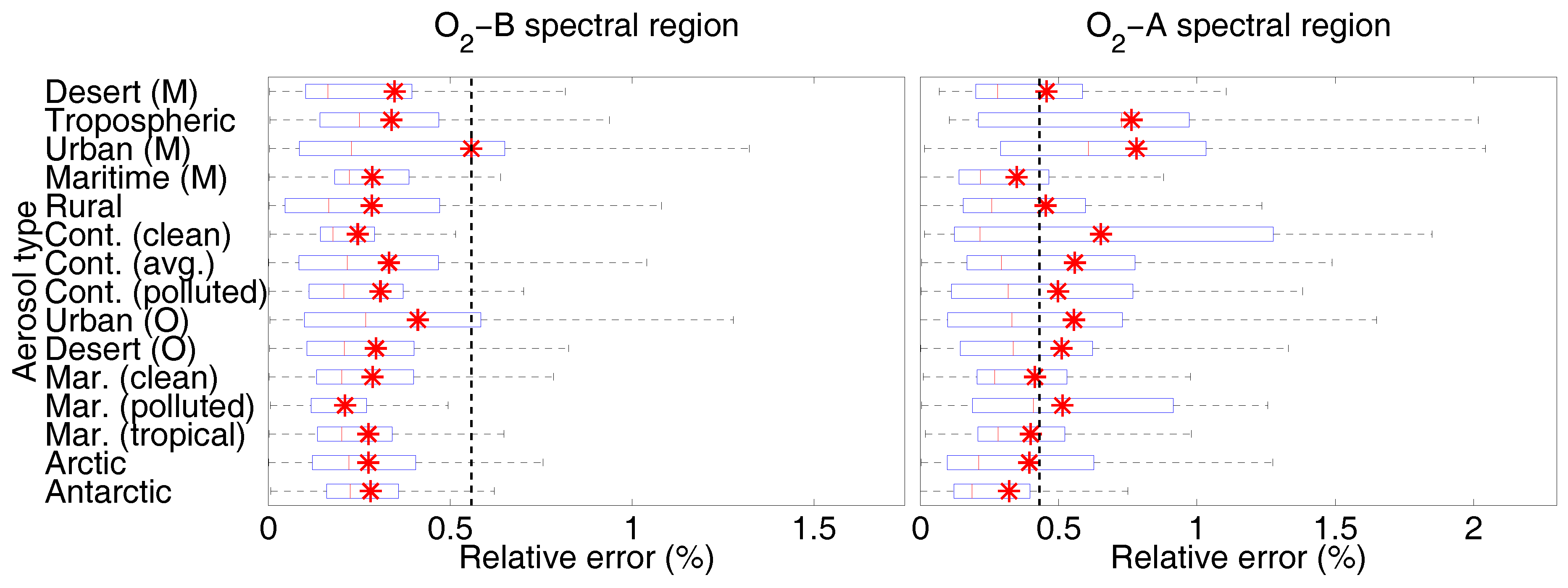
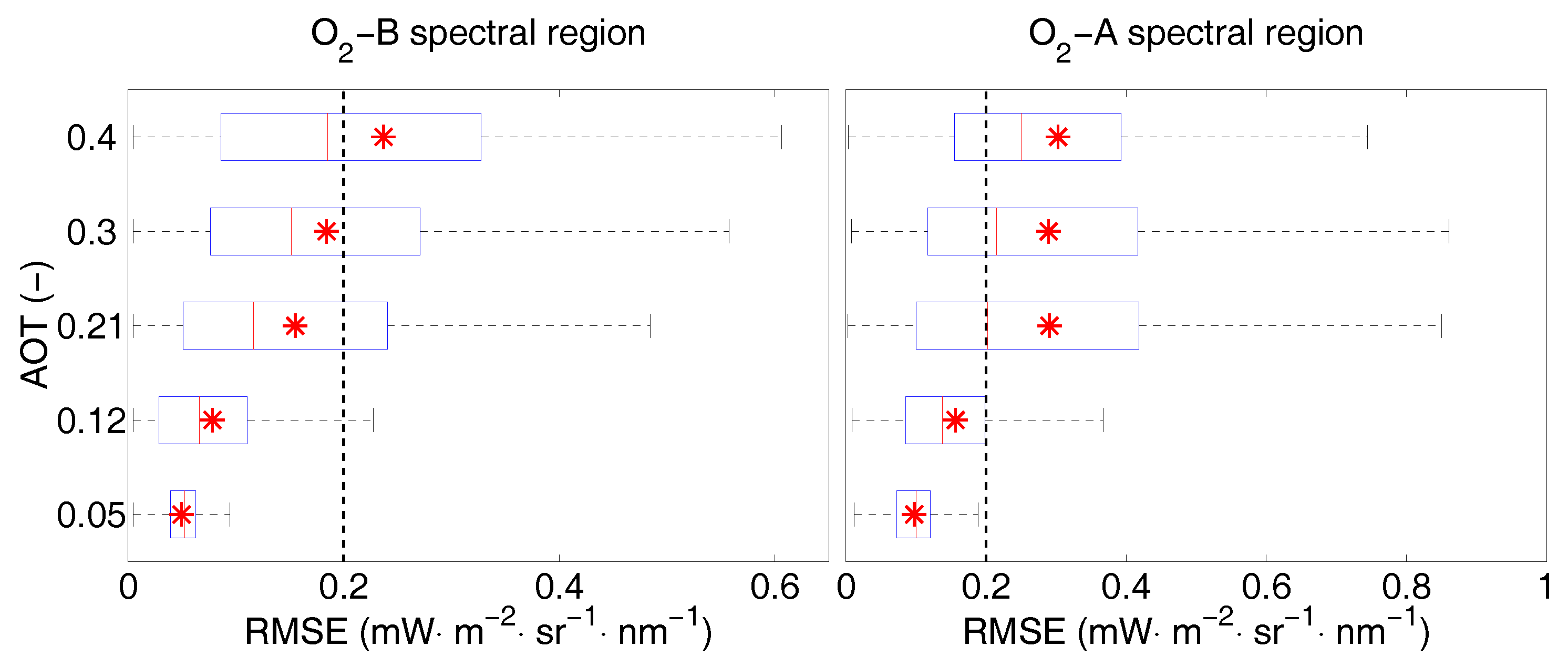
4.2. Apparent Reflectance Error Analysis Within Each O${}_2$ Absorption Band

Next, we evaluate the impact of approximations and assumptions on aerosol optical properties in atmospherically-corrected surface apparent reflectance. After the atmospheric correction using the complete retrieval dataset and its four subsets (see Table 4), we evaluate the mean relative error, averaged for all samples in the reference dataset (see Figure 7).

An aerosol characterization based solely on the variable AOT${}_{550}$ (subset #1, red line) does not compensate the variability in TOA radiance caused by all aerosol optical properties. The errors in surface apparent reflectance occur both inside and outside the O${}_2$ absorptions and particularly in the O${}_2$-B spectral region, where the scattering processes (and thus the phase function) have a larger influence. In agreement with the above GSA, the importance of ignoring the aerosol phase function can also be observed when using subset #4 (light blue line), which despite of considering 3 key aerosol parameters (i.e., AOT${}_{550}$, Ångström exponent and SSA), also results in high errors.

The influence of considering a spectrally-invariant SSA is also observed when comparing the errors obtained in the subset #2 (in dark blue, fixing the SSA) with those lower errors in the subset #3 (in orange, fixing the Ångström exponent). Again, the importance of scattering (through the SSA) is more prominent in shorter wavelengths, i.e., the difference between dark blue and orange lines is higher within the O${}_2$-B spectral region than within the O${}_2$-A.

Comparing the complete dataset (in green line) with subset #3 (fixing the Ångström exponent, in orange line), it seems that considering the Ångström exponent for the atmospheric characterization and retrieval hardly reduce the errors in the retrieved apparent reflectance.

The same trend appears when evaluating the number of samples in the reference dataset that are atmospherically-corrected within the error threshold (see

Table 5. Percentage of samples in the reference dataset with a retrieved surface apparent reflectance below the error threshold within the O${}_2$-B and O${}_2$-A bands.

	Subset #1	Subset #2	Subset #3	Subset #4	Complete
O${}_2$-B	19%	51%	63%	11%	85%
O${}_2$-A	22%	47%	53%	13%	59%

). The impact of ignoring the asymmetry parameter is observed in the lower accuracy of the retrievals in subsets #1 and #4 when compared against the other subsets (i.e., those including the HG parameter). While including the Ångström exponent hardly improves the results within the O${}_2$-A spectral range, it seems to improve the results within the O${}_2$-B spectral range, thereby increasing the percentage of samples atmospherically-corrected within the error threshold from 63% (with subset #3) up to 85% (with the complete retrieval dataset).

Next, in order to further determine the source of errors in the atmospheric correction, we show the relative errors propagated in apparent reflectance filtered by aerosol type (see Figure 8) and by AOT${}_{550}$ value (see Figure 9). We have calculated the error statistics for each of the filtered relative error values through box plots.

When filtered by aerosol type, it can be observed that the higher errors within the O${}_2$-B absorption region are given in both OPAC and MODTRAN urban aerosols, i.e., in highly absorbent aerosols with low SSA. However, the errors in this spectral region are on average below the threshold, which implies that the approximations and assumptions considered in the retrieval dataset are suitable for the atmospheric correction within the O${}_2$-B band.

As for the errors in the O${}_2$-A absorption region, again MODTRAN’s urban aerosol type shows the largest average error and the second largest 75th percentile. However, and opposite to the errors in the O${}_2$-B absorption, OPAC’s urban aerosol does not particularly lead to high error statistics. In addition, MODTRAN’s tropospheric and OPAC’s continental clean aerosols show high dispersion between low and high errors.

When filtered by AOT${}_{550}$, it can be observed that the errors in both O${}_2$ bands increase with higher aerosol loads (see Figure 9). Errors in the characterization and parameterization of key aerosol optical properties start to be propagated to the retrieved apparent reflectance at higher aerosol concentrations. However, nearly 85% of the reference dataset is atmospherically-corrected within the error threshold for typical AOT${}_{550}$ values of 0.05–0.21 [49,50].

Similar error statistics have been analyzed (box plots not presented) for the apparent reflectance errors filtered by the vertical aerosol distribution, however, in agreement with the GSA results in Section 4.1, vertical aerosol distribution does not play a significant role.

4.3. Retrieved Key Aerosol Optical Properties

Here we assess the accuracy of the implemented approximations on the retrieved key aerosol optical properties. We have first evaluated the errors in the retrieved AOT${}_{550}$ (see

Table 6. Evaluation of retrieved AOT${}_{550}$ against each reference dataset value.

Reference AOT${}_{\mathbf{550}}$ (-):	0.05	0.12	0.21	0.30	0.40
Retrieved AOT${}_{\mathbf{550}}$ (-):	0.04 ± 0.01	0.12 ± 0.03	0.24 ± 0.06	0.32 ± 0.06	0.38 ± 0.04

). These results indicate that, in average and despite the assumptions considered in the retrieval dataset, the AOT${}_{550}$ can be retrieved with a precision below 0.06 and with an error below 0.03 for all reference AOT${}_{550}$ values.

Secondly, as for the optical properties of OPAC aerosols implemented in the reference dataset, Figure 10 and Figure 11 show their spectral or angular dependency. In Figure 10 (left) we can observe that the extinction coefficients (normalized by their values at 550 nm) (circles) are well fitted (mean $R^2$ of 0.9973) by the Ångström law. In Figure 10 (right), the SSA shows a nearly constant spectral dependency in the 650–800 nm spectral range with maximum variations of 3% (for urban and desert aerosols).

The angular dependency of the various phase functions (at 700 nm) and their best fittings to a HG phase function is displayed in Figure 11 (left). Despite of the good parametric fitting (mean $R^2$ of 0.9854), the log-log scale shows that at forward scattering angles (0–10 deg), where the phase function is higher, the fitting is poorer, particularly for OPAC’s desert aerosol (in orange). Also, the spectral dependency of the asymmetry parameters shows variations below 2.5% in the 650–800 nm range (see Figure 11 (right)), which indicates that the asymmetry parameter can be considered spectrally invariant.

The retrieved aerosol optical properties are given in

Table 7. Evaluation of mean and standard deviation retrieved Ångström exponent, HG asymmetry parameter and SSA on OPAC aerosols. Reference values are given in bold font. Color code in the square symbols corresponds to those in Figure 10 and Figure 11.

Aerosol Type	Ångström Exponent	HG Asymmetry Parameter	SSA
Cont. (clean) ($\blacksquare$)	0.8 ± 0.3 (1.42)	0.67 ± 0.05 (0.82)	0.94 ± 0.06 (0.96)
Cont. (avg.) ($\blacksquare$)	0.8 ± 0.4 (1.42)	0.68 ± 0.04 (0.82)	0.92 ± 0.04 (0.90)
Cont. (polluted) ($\blacksquare$)	0.9 ± 0.6 (1.45)	0.67 ± 0.04 (0.79)	0.88 ± 0.04 (0.87)
Urban ($\blacksquare$)	0.9 ± 0.6 (1.43)	0.69 ± 0.05 (0.81)	0.84 ± 0.05 (0.78)
Desert ($\blacksquare$)	0.8 ± 0.5 (0.15)	0.69 ± 0.04 (0.91)	0.91 ± 0.05 (0.92)
Mar. (clean.) ($\blacksquare$)	0.9 ± 0.5 (0.09)	0.67 ± 0.04 (0.88)	0.96 ± 0.06 (0.997)
Mar. (polluted) ($\blacksquare$)	0.9 ± 0.4 (0.35)	0.68 ± 0.05 (0.87)	0.95 ± 0.06 (0.98)
Mar. (tropical) ($\blacksquare$)	0.9 ± 0.5 (0.05)	0.66 ± 0.04 (0.88)	0.96 ± 0.06 (0.998)
Arctic ($\blacksquare$)	0.8 ± 0.6 (0.9)	0.68 ± 0.04 (0.83)	0.87 ± 0.04 (0.88)
Antarctic ($\blacksquare$)	1.2 ± 0.5 (0.78)	0.66 ± 0.04 (0.75)	0.97 ± 0.05 (1)

. Each column displays the average and the standard deviation of the retrieved values for each OPAC aerosol within the reference dataset. The following observations can be made:

• Ångström exponent: the poor accuracy (0.6 average error) and the high dispersion (precision between 0.3 and 0.6) of the retrieved Ångström exponent for all aerosol types are noteworthy. This supports the results of the conducted GSA, i.e., that the Ångström exponent has a secondary order influence on the variability of the TOA radiance in the O${}_2$ wavelength range and thus the difficulty to derive its value just using FLORIS instrument. The low precision of the retrieved Ångström exponent indicates that this parameter has been used to compensate for variations on other aerosol optical properties (e.g., phase function and SSA).
• HG asymmetry parameter: we observe that an effective and spectrally-invariant HG asymmetry parameter of 0.68 ± 0.04 reproduces, overall, the main scattering processes related to the phase function. This indicates that the effect of aerosol scattering in the at-sensor TOA radiance is more related to illumination and observation geometry than to the aerosol type. Consequently, the variability of Mie phase functions implemented in the reference dataset can be compensated with an effective value of the HG asymmetry parameter for the given observation/illumination geometry. Though the HG approximation with an effective spectrally-invariant asymmetry parameter might be suitable within the O${}_2$-B spectral region, it plays a more important role inside the O${}_2$-A absorption band, which causes higher errors in apparent reflectance.
• Single scattering albedo: as with the retrieved AOT${}_{550}$, the retrieved values of SSA are in agreement (within the standard deviation) with the reference SSA values. This is true except for OPAC’s urban aerosol, which overestimates the SSA with an error of 0.06 ± 0.05, in agreement with the higher apparent reflectance error values within the O${}_2$-B spectral region seen in Figure 8 (left).

4.4. Propagation of Atmospheric Correction Errors Into Retrieved SIF within Each O${}_2$ Absorption Band

Finally, we have evaluated the error propagation of approximations and assumptions on aerosol optical properties into the retrieved SIF. Figure 12 evaluates, with a box plot diagram, the SIF error statistics, filtered by AOT${}_{550}$, after using the complete retrieval dataset for the atmospheric correction.

It can be observed that SIF can be retrieved with an error below 0.2 mW·m${}^{-2}·$sr${}^{-1}·$nm${}^{-1}$ in nearly 70% of the reference dataset for typical AOT${}_{550}$ values of 0.05–0.21. These results are in agreement with the errors derived in the surface apparent reflectance shown in Figure 9.

5. Discussion

The most important messages conveyed in this work, and the implications for the ESA’s FLEX/Sentinel-3 tandem mission data processing and further studies for atmospheric simulation can be summarized as follows.

5.1. Interpreting Atmospheric Correction Results: Implications for FLEX/Sentinel-3 Tandem Mission

A multi-parametric description of aerosol properties was applied in order to study its accuracy in the atmospheric correction of ESA’s FLEX/Sentinel-3 tandem mission. Overall, the results from the GSA reveal the importance of the scattering processes, particularly through the larger influence of aerosol phase function and SSA on the TOA radiance. These results are in agreement with our previous analysis in [46], where it was observed the high influence of the aerosol phase function, particularly on the diffuse terms of the TOA radiance in Equation (6) (i.e., $E_{dif}$, $T_{dif}$ and S). Previous studies such as [51,52] also indicate an increase of uncertainty in atmospheric correction due to errors related to a poor characterization of the aerosol phase function and SSA. A possible atmospheric correction strategy, e.g., as used in the Sentinel-3 SYN atmospheric correction algorithm [53], is to include a discrete set of aerosol types with predefined optical properties. However, various studies observed important discrepancies in aerosol optical properties between OPAC database and ground measurements ([54,55,56]), which indicate that discretization might not be accurate enough for an atmospheric correction. Instead, our atmospheric correction approach considers a multi-parametric approximation of aerosol properties with the assumption that effective aerosol variables can be mutually compensated to match the instrument TOA radiance data. We demonstrated that this approach achieves the required accuracy for FLEX atmospheric correction (SIF retrieval) in 85% (70%) of the considered cases for typical aerosol load conditions [49,50]. The analysis of the atmospheric correction results derive the following observations:

• Retrieving the aerosol phase function is important for an atmospheric correction scheme to enable compensating the variability of aerosol scattering in at-sensor TOA radiance. However, our results show that the spectrally-invariant HG approximation is adequate for the atmospheric correction of FLEX. Indeed, an effective HG asymmetry parameter describes the main scattering effects in TOA radiance associated to the phase function for aerosols of different type, which are mainly driven by the illumination/observation geometry.
• Our results indicate that only high SSA errors in highly absorbent aerosols (low SSA) might lead to an increase of the apparent reflectance error in the O${}_2$-B spectral region but not in the O${}_2$-A spectral region. In fact, as observed in the GSA results, the SSA has less influence inside of the O${}_2$-A absorption band and thus errors in the estimation of SSA will also have less impact in the atmospheric correction and on the SIF retrieval.
• The AOT${}_{550}$ is retrieved with a low error despite the implemented multi-parametric atmospheric correction. This is important in view of the possibility to evaluate the quality of FLEX atmospheric correction through the comparison of retrieved AOT${}_{550}$ against reference values (e.g., from the Aerosol Robotic Network (AERONET) [1,12]).
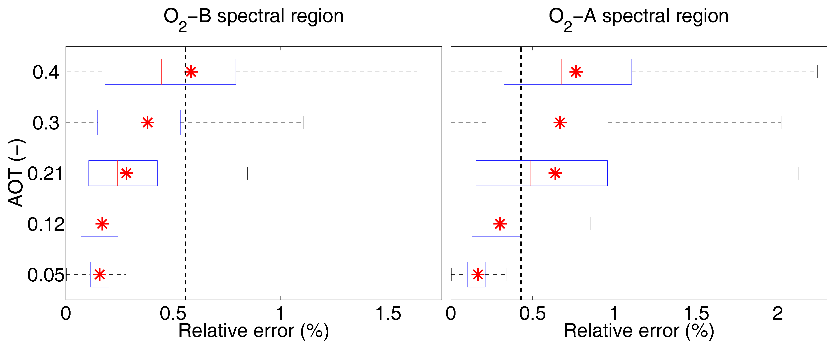
• When filtered by aerosol type, the errors on the retrieved apparent reflectance indicate that the assumption of spectrally-invariant asymmetry parameter and SSA might not be fully sufficient for all aerosol types. This is particularly relevant at aerosol concentrations with an AOT${}_{550}$ > 0.2, where errors in the characterization and the parameterization of key aerosol optical properties are propagated to the retrieved apparent reflectance and SIF within the O${}_2$-A spectral region.
• The error of atmospherically-corrected apparent reflectance is less affected by the variability of aerosol vertical profiles than the variability of aerosol optical properties. This was already observed in previous research [57] where, for nadir observations within the O${}_2$-A absorption region, aerosol vertical distribution was only retrieved over targets with low surface reflectance and at aerosol load conditions of AOT${}_{550}$ > 0.3. We can therefore conclude that assuming a predefined aerosol vertical distribution in FLEX atmospheric correction will not lead to a large error contribution to the retrieved apparent reflectance and subsequent SIF retrieval.
• The low precision of the retrieved Ångström exponent indicates that, on the one hand, this parameter cannot be retrieved from the short spectral range of FLORIS data. It justifies the use of the wider spectral range covered by Sentinel-3 instruments in this part. On the other hand, we observed that fixing the Ångström exponent (e.g., by inversion from Sentinel-3 data) will not have a large impact on the atmospheric correction accuracy within the O${}_2$ absorption region. However, an error in the Ångström exponent may lead to errors in surface reflectance in a wider spectral range that will be propagated to errors in retrieved SIF, especially when using Spectral Fitting Methods [58].

Based on these observations, we are developing a multi-parametric atmospheric characterization step for FLEX atmospheric correction algorithm that exploits the synergy of FLORIS, Ocean and Land Colour Instrument (OLCI) and Sea and Land Surface Temperature Radiometer (SLSTR) data.

5.2. New Opportunities for Atmospheric Simulation

To facilitate the simulation of large MODTRAN-based multi-dimensional look-up tables, we developed a software package called Atmospheric Look-up Table Generator (ALG). Although the generation of these multi-dimensional atmospheric look-up tables has been partially described in the past [35,59], tools are missing that allow their generation in a simple manner. For example, existing tools such as ONTAR’s PcModWin [60] or the official MODTRAN6 website [61] are limited to the execution of MODTRAN for a single combination of key input parameters. The generation of a multi-dimensional dataset would therefore require the impractical task of manually editing and running hundreds or thousands MODTRAN input files and process their generated output files into the final multi-dimensional dataset. Other commercial tools such as ReSe’s MODO [62] offer capabilities for sensitivity analysis through parameter series but the generation of multi-dimensional datasets is not easily achieved through its interface. The introduction of ALG allows users to: (1) define easily a wide variety of multiple combinations of key input parameters for the dataset, (2) run efficiently parallel execution of multiple instances of an atmospheric RTM as a third-party software and (3) process automatically the atmospheric RTM output data files and generating the final look-up table. The broader scientific community can subsequently use ALG (downloaded at http://ipl.uv.es/artmo/index.php/tools/80-tools/24-alg) for a wide variety of applications such as:

• Atmospheric correction: ALG facilitates users with the definition of atmospheric datasets that can be used for a physically-based atmospheric correction of satellite passive optical instruments [7,8,9,10].
• Cross-comparison of atmospheric RTMs: The modular design of the ALG tool allows expanding with additional atmospheric RTMs such as Second Simulation of a Satellite Signal in the Solar Spectrum-Vector (6SV) [63,64], which facilitates the cross-comparison of various atmospheric RTMs [65,66,67].
• Forward simulation: The generation of synthetic satellite data has been an active research field since the late 80 s [68]. As shown in recent satellite mission simulators ([69,70,71]), the generation of synthetic TOA radiance scenes play an important role to assess a mission performance. Through its datasets, ALG can extend the current simulation capabilities of satellite mission simulators to generate synthetic scenes in a large variety of atmospheric conditions. In combination with satellite mission simulators, ALG would allow scientists and engineers validating and optimizing satellite data processing schemes.
• Sensitivity analysis: As demonstrated in our previous study [46] and exploited in this paper, ALG and global sensitivity analysis can be used to identify the most influential atmospheric variables affecting satellite radiance data, which would serve as a tool to design new passive optical instruments.

6. Conclusions

Characterization of aerosol optical properties and vertical distribution are the main sources of error in the atmospheric correction of any satellite optical mission. Physically-based atmospheric correction algorithms rely on the implementation of assumptions or approximations with respect these aerosol characteristics. In this paper, we studied the accuracy of using approximations and assumptions related to aerosol properties to describe their net radiometric effects through their impact in synthetic atmospherically-corrected FLORIS data and subsequent retrieved Sun-induced Fluorescence (SIF). To do that, we used a newly developed Atmospheric Look-up Table Generator (ALG) tool to simulate three synthetic datasets based on the execution of MODTRAN RTM coupled with OPAC aerosol database. Unlike the commonly used strategy of discretizing aerosol optical properties by aerosol types, we demonstrated that a multi-parametric aerosol characterization based on effective variables is sufficient for the atmospheric correction of ESA’s FLEX mission data. Especially, characterizing scattering effects can play an important role in an accurate atmospheric correction algorithm. However, the approximations of (1) a spectrally-invariant Henyey-Greenstein asymmetry parameter and (2) a spectrally-invariant single scattering albedo already account for the main scattering processes in the 650–780 nm range. We also demonstrated that errors in the effective Ångström exponent retrieved from the wider spectral range covered by Sentinel-3 OLCI and SLSTR instruments, flying in tandem with FLEX, has negligible impact within the O${}_2$ regions. In addition, we found that the aerosol vertical distribution has a marginal influence on the TOA radiance for this type of satellite observations. This suggests that a predefined standard aerosol vertical distribution is appropriate to realize an accurate atmospheric correction of FLEX data. Altogether, the implemented approximations reach the required accuracy in the atmospheric correction of ESA’s FLEX mission (and SIF retrieval) in nearly 85% (70%) of the considered cases with typical aerosol load conditions (i.e., AOT${}_{550}$ < 0.2).

References

1. Kokhanovsky, A.; Breon, F.M.; Cacciari, A.; Carboni, E.; Diner, D.; Di Nicolantonio, W.; Grainger, R.; Grey, W.; Höller, R.; Lee, K.H.; et al. Aerosol remote sensing over land: A comparison of satellite retrievals using different algorithms and instruments. Atmos. Res. 2007, 85, 372–394. [Google Scholar] [CrossRef]
2. Schaepman, M.; Ustin, S.; Plaza, A.; Painter, T.; Verrelst, J.; Liang, S. Earth system science related imaging spectroscopy-An assessment. Remote Sens. Environ. 2009, 113, S123–S137. [Google Scholar] [CrossRef]
3. Gao, B.C.; Montes, M.; Davis, C.; Goetz, A. Atmospheric correction algorithms for hyperspectral remote sensing data of land and ocean. Remote Sens. Environ. 2009, 113, S17–S24. [Google Scholar] [CrossRef]
4. Verrelst, J.; Camps-Valls, G.; Muñoz-Marí, J.; Rivera, J.; Veroustraete, F.; Clevers, J.; Moreno, J. Optical remote sensing and the retrieval of terrestrial vegetation bio-geophysical properties—A review. ISPRS J. Photogramm. Remote Sens. 2015, 108, 273–290. [Google Scholar] [CrossRef]
5. Chavez, P., Jr. Image-based atmospheric corrections—Revisited and improved. Photogramm. Eng. Remote Sens. 1996, 62, 1025–1036. [Google Scholar]
6. Bernstein, L.; Jin, X.; Gregor, B.; Adler-Golden, S. Quick atmospheric correction code: Algorithm description and recent upgrades. Opt. Eng. 2012, 51, 111719. [Google Scholar] [CrossRef]
7. Cooley, T.; Anderson, G.; Felde, G.; Hoke, M.; Ratkowski, A.; Chetwynd, J.; Gardner, J.; Adler-Golden, S.; Matthew, M.; Berk, A.; et al. FLAASH, a MODTRAN4-based atmospheric correction algorithm, its applications and validation. In Proceedings of the IEEE International Coference on Geoscience and Remote Sensing Symposium, Toronto, ON, Canada, 24–28 June 2002; Volume 3, pp. 1414–1418. [Google Scholar]
8. Richter, R.; Schläpfer, D. Geo-atmospheric processing of airborne imaging spectrometry data. Part 2: Atmospheric/topographic correction. Int. J. Remote Sens. 2002, 23, 2631–2649. [Google Scholar] [CrossRef]
9. Guanter, L.; González-Sanpedro, M.D.C.; Moreno, J. A method for the atmospheric correction of ENVISAT/MERIS data over land targets. Int. J. Remote Sens. 2007, 28, 709–728. [Google Scholar] [CrossRef]
10. North, P.; Brockmann, C.; Fischer, J.; Gomez-Chova, L.; Grey, W.; Heckel, A.; Moreno, J.; Preusker, R.; Regner, P. Meris/AATSR Synergy Algorithms for Cloud Screening, Aerosol Retrieval and Atmospheric Correction. In Proceedings of the 2nd MERIS/AATSR User Workshop, ESA, Frascati, Italy, 22–26 September 2008. [Google Scholar]
11. Inness, A.; Baier, F.; Benedetti, A.; Bouarar, I.; Chabrillat, S.; Clark, H.; Clerbaux, C.; Coheur, P.; Engelen, R.; Errera, Q.; et al. The MACC reanalysis: An 8 yr data set of atmospheric composition. Atmos. Chem. Phys. 2013, 13, 4073–4109. [Google Scholar] [CrossRef]
12. Holben, B.; Eck, T.; Slutsker, I.; Tanré, D.; Buis, J.; Setzer, A.; Vermote, E.; Reagan, J.; Kaufman, Y.; Nakajima, T.; et al. AERONET—A federated instrument network and data archive for aerosol characterization. Remote Sens. Environ. 1998, 66, 1–16. [Google Scholar] [CrossRef]
13. Schläpfer, D.; Borel, C.; Keller, J.; Itten, K. Atmospheric precorrected differential absorption technique to retrieve columnar water vapor. Remote Sens. Environ. 1998, 65, 353–366. [Google Scholar] [CrossRef]
14. Marbach, T.; Phillips, P.; Lacan, A.; Schlüssel, P. The Multi-Viewing, -Channel, -Polarisation Imager (3MI) of the EUMETSAT Polar System—Second Generation (EPS-SG) Dedicated to Aerosol Characterisation. In Proceedings of the SPIE 8889, Sensors, Systems, and Next-Generation Satellites XVII, 88890, Dresden, Germany, 16 October 2013; Volume 8889. [Google Scholar]
15. Young, S.; Vaughan, M. The retrieval of profiles of particulate extinction from cloud-aerosol lidar infrared pathfinder satellite observations (CALIPSO) data: Algorithm description. J. Atmos. Ocean. Technol. 2009, 26, 1105–1119. [Google Scholar] [CrossRef]
16. Hess, M.; Koepke, P.; Schult, I. Optical Properties of Aerosols and Clouds: The Software Package OPAC. Bull. Am. Meteorol. Soc. 1998, 79, 831–844. [Google Scholar] [CrossRef]
17. Dubovik, O.; Holben, B.; Eck, T.; Smirnov, A.; Kaufman, Y.; King, M.; Tanré, D.; Slutsker, I. Variability of absorption and optical properties of key aerosol types observed in worldwide locations. J. Atmos. Sci. 2002, 59, 590–608. [Google Scholar] [CrossRef]
18. Mishra, A.; Koren, I.; Rudich, Y. Effect of aerosol vertical distribution on aerosol-radiation interaction: A theoretical prospect. Heliyon 2015, 1. [Google Scholar] [CrossRef] [PubMed]
19. Duforêt, L.; Frouin, R.; Dubuisson, P. Importance and estimation of aerosol vertical structure in satellite ocean-color remote sensing. Appl. Opt. 2007, 46, 1107–1119. [Google Scholar] [CrossRef] [PubMed]
20. European Space Agency (ESA). Report for Mission Selection: FLEX; ESA SP-1330/2 (2 Volume Series); European Space Agency: Noordwijk, The Netherlands, 2015. [Google Scholar]
21. Drusch, M.; Moreno, J.; Del Bello, U.; Franco, F.; Goulas, Y.; Huth, A.; Kraft, S.; Middleton, E.M.; Miglietta, F.; Mohammed, G.; et al. The FLuorescence EXplorer Mission Concept-ESA’s Earth Explorer 8. IEEE Trans. Geosci. Remote Sens. 2016, 55, 1–12. [Google Scholar] [CrossRef]
22. Kraft, S.; Bézy, J.L.; Del Bello, U.; Berlich, R.; Drusch, M.; Franco, R.; Gabriele, A.; Harnisch, B.; Meynart, R.; Silvestrin, P. FLORIS: Phase A status of the fluorescence imaging spectrometer of the earth explorer mission Candidate FLEX. Proc. SPIE Int. Soc. Opt. Eng. 2013, 8889. [Google Scholar] [CrossRef]
23. Donlon, C.; Berruti, B.; Buongiorno, A.; Ferreira, M.H.; Féménias, P.; Frerick, J.; Goryl, P.; Klein, U.; Laur, H.; Mavrocordatos, C.; et al. The Global Monitoring for Environment and Security (GMES) Sentinel-3 mission. Remote Sens. Environ. 2012, 120, 37–57. [Google Scholar] [CrossRef]
24. Angström, A. On the Atmospheric Transmission of Sun Radiation and on Dust in the Air. Geogr. Ann. 1929, 11, 156–166. [Google Scholar] [CrossRef]
25. Eck, T.; Holben, B.; Reid, J.; Dubovik, O.; Smirnov, A.; O’Neill, N.; Slutsker, I.; Kinne, S. Wavelength dependence of the optical depth of biomass burning, urban, and desert dust aerosols. J. Geophys. Res. Atmos. 1999, 104, 31333–31349. [Google Scholar] [CrossRef]
26. Mie, G. Beiträge zur Optik trüber Medien, speziell kolloidaler Metallösungen. Annal. Phys. 1908, 330, 377–445. [Google Scholar] [CrossRef]
27. Henyey, L.; Greenstein, J. Diffuse radiation in the galaxy. Astrophys. J. 1941, 93, 70–83. [Google Scholar] [CrossRef]
28. Toon, O.; Pollack, J. A Global Average Model of Atmospheric Aerosols for Radiative Transfer Calculations. J. Appl. Meteorol. 1976, 15, 225–246. [Google Scholar] [CrossRef]
29. Léon, J.F.; Derimian, Y.; Chiapello, I.; Tanré, D.; Podvin, T.; Chatenet, B.; Diallo, A.; Deroo, C. Aerosol vertical distribution and optical properties over M’Bour (16.96 W;14.39 N), Senegal from 2006 to 2008. Atmos. Chem. Phys. 2009, 9, 9249–9261. [Google Scholar] [CrossRef]
30. Christensen, J. The Danish eulerian hemispheric model—A three-dimensional air pollution model used for the arctic. Atmos. Environ. 1997, 31, 4169–4191. [Google Scholar] [CrossRef]
31. Berk, A.; Anderson, G.; Acharya, P.; Bernstein, L.; Muratov, L.; Lee, J.; Fox, M.; Adler-Golden, S.; Chetwynd, J.; Hoke, M.; et al. MODTRANTM 5: 2006 Update. In Proceedings of the SPIE 6233, Algorithms and Technologies for Multispectral, Hyperspectral, and Ultraspectral Imagery XII, 62331F, Orlando (Kissimmee), FL, USA, 8 May 2016; Volume 6233 II. [Google Scholar]
32. Pedrós, R.; Gómez-Amo, J.; Marcos, C.; Utrillas, M.; Gandía, S.; Tena, F.; Lozano, J. AEROgui: A graphical user interface for the optical properties of aerosols. Bull. Am. Meteorol. Soc. 2014, 95, 1863–1871. [Google Scholar] [CrossRef]
33. McKay, M.; Beckman, R.; Conover, W. Comparison of three methods for selecting values of input variables in the analysis of output from a computer code. Technometrics 1979, 21, 239–245. [Google Scholar] [CrossRef]
34. Huang, F.; Zhou, J.; Tao, J.; Tan, X.; Liang, S.; Cheng, J. PMODTRAN: A parallel implementation based on MODTRAN for massive remote sensing data processing. Int. J. Dig. Earth 2016, 9, 819–834. [Google Scholar] [CrossRef]
35. Guanter, L.; Richter, R.; Kaufmann, H. On the application of the MODTRAN4 atmospheric radiative transfer code to optical remote sensing. Int. J. Remote Sens. 2009, 30, 1407–1424. [Google Scholar] [CrossRef]
36. Berk, A.; Bernstein, L.; Anderson, G.; Acharya, P.; Robertson, D.; Chetwynd, J.; Adler-Golden, S. MODTRAN cloud and multiple scattering upgrades with application to AVIRIS. Remote Sens. Environ. 1998, 65, 367–375. [Google Scholar] [CrossRef]
37. Thome, K.; Palluconi, F.; Takashima, T.; Masuda, K. Atmospheric correction of ASTER. IEEE Trans. Geosci. Remote Sens. 1998, 36, 1199–1211. [Google Scholar] [CrossRef]
38. Settle, J. On the dimensionality of multi-view hyperspectral measurements of vegetation. Remote Sens. Environ. 2004, 90, 235–242. [Google Scholar] [CrossRef]
39. Saltelli, A.; Tarantola, S.; Chan, K.S. A quantitative model-independent method for global sensitivity analysis of model output. Technometrics 1999, 41, 39–56. [Google Scholar] [CrossRef]
40. Verrelst, J.; Rivera, J.; Van Der Tol, C.; Magnani, F.; Mohammed, G.; Moreno, J. Global sensitivity analysis of the SCOPE model: what drives simulated canopy-leaving sun-induced fluorescence? Remote Sens. Environ. 2015, 166, 8–21. [Google Scholar] [CrossRef]
41. Verrelst, J.; van der Tol, C.; Magnani, F.; Sabater, N.; Rivera, J.; Mohammed, G.; Moreno, J. Evaluating the predictive power of sun-induced chlorophyll fluorescence to estimate net photosynthesis of vegetation canopies: A SCOPE modeling study. Remote Sens. Environ. 2016, 176, 139–151. [Google Scholar] [CrossRef]
42. Saltelli, A.; Annoni, P.; Azzini, I.; Campolongo, F.; Ratto, M.; Tarantola, S. Variance based sensitivity analysis of model output. Design and estimator for the total sensitivity index. Comput. Phys. Commun. 2010, 181, 259–270. [Google Scholar] [CrossRef]
43. Van Der Tol, C.; Verhoef, W.; Timmermans, J.; Verhoef, A.; Su, Z. An integrated model of soil-canopy spectral radiances, photosynthesis, fluorescence, temperature and energy balance. Biogeosciences 2009, 6, 3109–3129. [Google Scholar] [CrossRef]
44. Van der Tol, C.; Berry, J.A.; Campbell, P.K.E.; Rascher, U. Models of fluorescence and photosynthesis for interpreting measurements of solar-induced chlorophyll fluorescence. J. Geophys. Res. Biogeosci. 2014, 119, 2312–2327. [Google Scholar] [CrossRef] [PubMed]
45. O’Hagan, A. Bayesian analysis of computer code outputs: A tutorial. Reliab. Eng. Syst. Saf. 2006, 91, 1290–1300. [Google Scholar] [CrossRef]
46. Verrelst, J.; Sabater, N.; Rivera, J.; Muñoz Marí, J.; Vicent, J.; Camps-Valls, G.; Moreno, J. Emulation of leaf, canopy and atmosphere radiative transfer models for fast global sensitivity analysis. Remote Sens. 2016, 8, 673. [Google Scholar] [CrossRef]
47. Meroni, M.; Busetto, L.; Colombo, R.; Guanter, L.; Moreno, J.; Verhoef, W. Performance of Spectral Fitting Methods for vegetation fluorescence quantification. Remote Sens. Environ. 2010, 114, 363–374. [Google Scholar] [CrossRef]
48. FLEX MAG; Drusch, M. FLEX Mission Requirements Document (MRD), v1.0; Technical Report; European Space Agency (ESA): Noordwijk, The Netherlands, 2011. [Google Scholar]
49. Lynch, P.; Reid, J.; Westphal, D.; Zhang, J.; Hogan, T.; Hyer, E.; Curtis, C.; Hegg, D.; Shi, Y.; Campbell, J.; et al. An 11-year global gridded aerosol optical thickness reanalysis (v1.0) for atmospheric and climate sciences. Geosci. Model Dev. 2016, 9, 1489–1522. [Google Scholar] [CrossRef]
50. Geogdzhayev, I.; Mishchenko, M.; Li, J.; Rossow, W.; Liu, L.; Cairns, B. Extension and statistical analysis of the GACP aerosol optical thickness record. Atmos. Res. 2015, 164–165, 268–277. [Google Scholar] [CrossRef]
51. Corradini, S.; Cervino, M. Aerosol extinction coefficient profile retrieval in the oxygen A-band considering multiple scattering atmosphere. Test case: SCIAMACHY nadir simulated measurements. J. Quant. Spectrosc. Radiat. Transf. 2006, 97, 354–380. [Google Scholar] [CrossRef]
52. Davies, W.; North, P. Synergistic angular and spectral estimation of aerosol properties using CHRIS/PROBA-1 and simulated Sentinel-3 data. Atmos. Meas. Tech. 2015, 8, 1719–1731. [Google Scholar] [CrossRef]
53. North, P.; Heckel, A. Sentinel-3 Optical Products and Algorithm Definition—SYN Algorithm Theoretical Basis Document; Technical Report; Swanswa University Prifysgol Abertawe: Swansea, UK, 2009. [Google Scholar]
54. Emde, C.; Buras, R.; Mayer, B.; Blumthaler, M. The impact of aerosols on polarized sky radiance: Model development, validation, and applications. Atmos. Chem. Phys. 2010, 10, 383–396. [Google Scholar] [CrossRef]
55. Zieger, P.; Fierz-Schmidhauser, R.; Weingartner, E.; Baltensperger, U. Effects of relative humidity on aerosol light scattering: Results from different European sites. Atmos. Chem. Phys. 2013, 13, 10609–10631. [Google Scholar] [CrossRef]
56. Di Biagio, C.; Boucher, H.; Caquineau, S.; Chevaillier, S.; Cuesta, J.; Formenti, P. Variability of the infrared complex refractive index of African mineral dust: Experimental estimation and implications for radiative transfer and satellite remote sensing. Atmos. Chemis. Phys. 2014, 14, 11093–11116. [Google Scholar] [CrossRef]
57. Dubuisson, P.; Frouin, R.; Dessailly, D.; Duforêt, L.; Léon, J.F.; Voss, K.; Antoine, D. Estimating the altitude of aerosol plumes over the ocean from reflectance ratio measurements in the O2 A-band. Remote Sens. Environ. 2009, 113, 1899–1911. [Google Scholar] [CrossRef]
58. Cogliati, S.; Verhoef, W.; Kraft, S.; Sabater, N.; Alonso, L.; Vicent, J.; Moreno, J.; Drusch, M.; Colombo, R. Retrieval of sun-induced fluorescence using advanced spectral fitting methods. Remote Sens. Environ. 2015, 169, 344–357. [Google Scholar] [CrossRef]
59. Brazile, J.; Richter, R.; Schläpfer, D.; Schaepman, M.; Itten, K. Cluster versus grid for operational generation of ATCOR’s modtran-based look up tables. Parallel Comput. 2008, 34, 32–46. [Google Scholar] [CrossRef]
60. Coorporation, O. PcModWin Official Webpage. Available online: http://www.ontar.com/Software/ProductDetails.aspx?item=PcModWin. (accessed on 27 December 2016).
61. Spectral Sciences Incorporated. Official MODTRAN6 Webpage. Available online: http://modtran.spectral.com/ (accessed on 27 December 2016).
62. ReSe Applications Schläpfer. MODO Official Webpage. Available online: http://www.rese.ch/products/modo/ ( accessed on 27 December 2016).
63. Kotchenova, S.; Vermote, E.; Matarrese, R.; Klemm, F., Jr. Validation of a vector version of the 6S radiative transfer code for atmospheric correction of satellite data. Part I: Path radiance. Appl. Opt. 2006, 45, 6762–6774. [Google Scholar] [CrossRef] [PubMed]
64. Kotchenova, S.; Vermote, E. Validation of a vector version of the 6S radiative transfer code for atmospheric correction of satellite data. Part II. Homogeneous Lambertian and anisotropic surfaces. Appl. Opt. 2007, 46, 4455–4464. [Google Scholar] [CrossRef] [PubMed]
65. Kotchenova, S.; Vermote, E.; Levy, R.; Lyapustin, A. Radiative transfer codes for atmospheric correction and aerosol retrieval: Intercomparison study. Appl. Opt. 2008, 47, 2215–2226. [Google Scholar] [CrossRef] [PubMed]
66. Seidel, F.; Kokhanovsky, A.; Schaepman, M. Fast and simple model for atmospheric radiative transfer. Atmos. Meas. Tech. 2010, 3, 1129–1141. [Google Scholar] [CrossRef]
67. Callieco, F.; Dell’Acqua, F. A comparison between two radiative transfer models for atmospheric correction over a wide range of wavelengths. Int. J. Remote Sens. 2011, 32, 1357–1370. [Google Scholar] [CrossRef]
68. Kerekes, J.P.; Landgrebe, D.A. Simulation of optical remote sensing systems. IEEE Trans. Geosci. Remote Sens. 1989, 27, 762–771. [Google Scholar] [CrossRef]
69. Dangel, S.; Schaepman, M.; Brazile, J.; Petitcolin, F.; Su, B.; Briottet, X.; Gloor, M.; Moreno, J.; Itten, K. System architecture and design for a SPECTRA mission end-to-end simulator. In Proceedings of SPECTRA Workshop; Noordwijk, Netherlands, October 2003, Volume 1, Available online: http://www.geo.uzh.ch/microsite/rsl-documents/research/publications/other-sci-communications/2004_SPECTRASim_ESA_SD-4044586752/2004_SPECTRASim_ESA_SD.pdf.
70. Segl, K.; Guanter, L.; Rogass, C.; Kuester, T.; Roessner, S.; Kaufmann, H.; Sang, B.; Mogulsky, V.; Hofer, S. EeteS—The EnMAP end-to-end simulation tool. IEEE J. Sel. Top. Appl. Earth Obs. Remote Sens. 2012, 5, 522–530. [Google Scholar] [CrossRef]
71. Vicent, J.; Sabater, N.; Tenjo, C.; Acarreta, J.; Manzano, M.; Rivera, J.; Jurado, P.; Franco, R.; Alonso, L.; Verrelst, J.; et al. FLEX End-to-End Mission Performance Simulator. IEEE Trans. Geosci. Remote Sens. 2016, 54, 4215–4223. [Google Scholar] [CrossRef]
Figure 1. Modular architecture of the developed ALG software tool.
Remotesensing 09 00675 g001
Figure 2. Screen-capture of the ALG (v1.0) tool at the LUT key input parameters configuration step.
Remotesensing 09 00675 g002
Figure 3. Reference Lambertian surface reflectance (left) and isotropic SIF emission (right).
Remotesensing 09 00675 g003
Figure 4. Approach for evaluating the impact of approximations in aerosol properties in FLORIS atmospherically-corrected surface reflectance.
Remotesensing 09 00675 g004
Figure 5. Relative error threshold in apparent reflectance in the O 2 -B (left) and O 2 -A (right) regions based on an increase of fluorescence of 0.2 mW·m 2 · sr 1 · nm 1 .
Remotesensing 09 00675 g005
Figure 6. Global sensitivity analysis for the O 2 -B (left) and O 2 -A (right) spectral regions.
Remotesensing 09 00675 g006
Figure 7. Mean relative error in surface apparent reflectance derived from the retrieval dataset and its four subsets (see Table 4) within the O 2 -B (left) and O 2 -A (right) spectral regions. The figure legend includes the ranging key input aerosol variables within each subset.
Remotesensing 09 00675 g007
Figure 8. Relative error in apparent reflectance, filtered by aerosol type, derived from the complete retrieval dataset within the O 2 -B (left) and O 2 -A (right) spectral regions. The following error statistic are provided: median ( | ), average ( ), 25th and 75th percentiles (blue boxes) and extreme min/max values (horizontal dashed lines). The vertical dashed line indicates the error threshold in apparent reflectance within each O 2 absorption. Notice that aerosol types with same name are indentified as MODTRAN (M) or OPAC (O).
Remotesensing 09 00675 g008
Figure 9. Relative error in apparent reflectance, filtered by AOT 550 , derived from the complete retrieval dataset within the O 2 -B (left) and O 2 -A (right) spectral regions. The following error statistics are provided: median ( | ), average ( ), 25th and 75th percentiles (blue boxes) and extreme min/max values (horizontal dashed lines). The vertical dashed line indicates the error threshold in apparent reflectance within each O 2 absorption.
Remotesensing 09 00675 g009
Figure 10. Default OPAC aerosols’ optical properties. (Left) normalized extinction coefficient (circles) and best fitting to Ångström law (dashed lines). (Right) wavelength dependency of SSA.
Remotesensing 09 00675 g010
Figure 11. (Left) phase function at 700 nm (solid lines) and best fitting to HG approximation (dashed lines). (Right) wavelength dependency of asymmetry parameter.
Remotesensing 09 00675 g011
Figure 12. Mean error statistic in retrieved SIF, filtered by AOT 550 , after the atmospheric correction of the reference dataset derived from the complete retrieval dataset within the O 2 -B (left) and O 2 -A (right) spectral regions. The following error statistic are provided: median ( | ), average ( ), 25th and 75th percentiles (blue boxes) and extreme min/max values (horizontal dashed lines). The vertical dashed line indicates the error threshold in SIF.
Remotesensing 09 00675 g012