Article

Estimating Chlorophyll Fluorescence Parameters Using the Joint Fraunhofer Line Depth and Laser-Induced Saturation Pulse (FLD-LISP) Method in Different Plant Species

by
Parinaz Rahimzadeh-Bajgiran
1,2,
Bayaer Tubuxin
1 and
Kenji Omasa
1,*
1
Graduate School of Agricultural and Life Sciences, The University of Tokyo, 1-1-1 Yayoi, Bunkyo-ku, Tokyo 113-8657, Japan
2
School of Forest Resources, University of Maine, 5755 Nutting Hall, Orono, ME 04469, USA
*
Author to whom correspondence should be addressed.
Remote Sens. 2017, 9(6), 599; https://doi.org/10.3390/rs9060599
Submission received: 5 January 2017 / Revised: 7 June 2017 / Accepted: 9 June 2017 / Published: 13 June 2017

Abstract

:
A comprehensive evaluation of the recently developed Fraunhofer line depth (FLD) and laser-induced saturation pulse (FLD-LISP) method was conducted to measure chlorophyll fluorescence (ChlF) parameters of the quantum yield of photosystem II (ΦPSII), non-photochemical quenching (NPQ), and the photosystem II-based electron transport rate (ETR) in three plant species including paprika (C3 plant), maize (C4 plant), and pachira (C3 plant). First, the relationships between photosynthetic photon flux density (PPFD) and ChlF parameters retrieved using FLD-LISP and the pulse amplitude-modulated (PAM) methods were analyzed for all three species. Then the relationships between ChlF parameters measured using FLD-LISP and PAM were evaluated for the plants in different growth stages of leaves from mature to aging conditions. The relationships of ChlF parameters/PPFD were similar in both FLD-LISP and PAM methods in all plant species. ΦPSII showed a linear relationship with PPFD in all three species whereas NPQ was found to be linearly related to PPFD in paprika and maize, but not for pachira. The ETR/PPFD relationship was nonlinear with increasing values observed for PPFDs lower than about 800 μmol m−2 s−1 for paprika, lower than about 1200 μmol m−2 s−1 for maize, and lower than about 800 μmol m−2 s−1 for pachira. The ΦPSII, NPQ, and ETR of both the FLD-LISP and PAM methods were very well correlated (R2 = 0.89, RMSE = 0.05), (R2 = 0.86, RMSE = 0.44), and (R2 = 0.88, RMSE = 24.69), respectively, for all plants. Therefore, the FLD-LISP method can be recommended as a robust technique for the estimation of ChlF parameters.

Graphical Abstract

1. Introduction

Chlorophyll (Chl) fluorescence (ChlF) measurement is a powerful non-destructive technique used to assess the photosynthetic performance of plants [1,2,3,4,5,6]. Various studies were conducted on the active measurement of ChlF signals using single point measurements [7,8,9,10,11,12] or ChlF imaging [13,14,15,16,17,18,19,20,21,22,23]. The ChlF principle is based on how light energy, which is absorbed by photosynthetic pigments such as chlorophylls and cartenoids is distributed [10]. Light energy received by Chl a has three main alternative fates; being used in photochemistry, being lost as non-radiative heat dissipation, or being emitted as fluorescence. By measuring ChlF, the efficiency of photochemistry and heat dissipation can be assessed [24]. ChlF offers a direct approach for actual plant photosynthetic activity measurement compared to reflectance measurements of vegetation captured by passive remote sensing sensors. In addition, plant stresses can be detected before visible signs of plant tissue deterioration or significant reduction in Chl content occurs [25,26,27].
The red and near-infrared (NIR) emissions by Chl coupled with quenching mechanisms have been used to estimate photosynthetic levels for decades. The process of “quenching”, occurs through photochemical and non-photochemical mechanisms. The active and passive remote sensing of ChlF was also frequently applied to detect plant stress on both leaf and canopy scales [16,28,29,30,31,32,33,34,35].
By the development of active techniques based on the pulse amplitude-modulated (PAM) method, effective measurement of ChlF outside the laboratory became possible [12]. The PAM technique with saturating light pulses allows the estimation of several ChlF parameters such as dark-adapted and light-adapted peak fluorescence (Fm and Fm’, respectively) and steady-state ChlF (Fs) to estimate the quantum yield of photosystem II (ΦPSII), the non-photochemical quenching (NPQ), and the photosystem II-based electron transport rate (ETR). ΦPSII, NPQ, and ETR are three widely used ChlF parameters, which are employed to measure photochemistry and the overall photosynthetic capacity of plants [9,24].
However, the PAM fluorometry method is limited to short-distance applications for individual leaves and small plants attributed to the need for an artificial saturation light pulse and accurate pulse-synchronized and modulated fluorimetric techniques. A method based on the laser induced Chl fluorescence transients (LIFT) was introduced as a tool to expand the application of active ChlF measurement methods to long-distance, canopy-scale studies [36,37]. In this approach, low-intensity pulses, instead of a saturating pulse, are used to measure the fluorescence transient, which is interpolated to a maximum fluorescence level using a fluorescence model. Using LIFT, ChlF can be measured up to a distance of 50 m but there are still challenges for longer distance remote sensing applications using this method [36,38,39].
To address ChlF measurement shortcomings on larger scales, passive remote sensing of steady-state solar-induced ChlF (SIF) has recently attracted more attention [27]. The advantage of the SIF method is that the technique does not require accurate pulse-synchronized and modulated fluorimetric techniques as needed in the PAM and LIFT methods. The Fraunhofer line depth (FLD) method [40] is the most widely used SIF technique to measure ChlF emission under solar light. Using the FLD method, absolute variations in steady-state ChlF can be estimated but ChlF parameters cannot be retrieved and consequently ETR cannot be estimated. At the ground level, two broad oxygen absorption bands of terrestrial atmosphere at 760 nm (O2A) and 686 nm (O2B) are usually used to estimate the steady-state SIF. These wavelengths can be used for SIF measurement on the ground and for low flying aircraft. For satellite observation, other wavelengths in the near-infrared region are recommended [41]. SIF signals can be measured as a proxy of photosynthesis from air-borne devices for canopy and larger scale applications [27,34,42,43,44,45,46,47,48,49,50,51]. More recently, the development of space-borne SIF remote sensing capability of the GOSAT (Greenhouse gases Observing SATellite) has provided the opportunity for SIF measurement from space [26,52] and for global mapping of SIF in the far-red region from satellites [41,53,54,55,56]. The application of SIF to assess the global terrestrial carbon cycle through the gross primary production (GPP) estimation has increasingly drawn attention and several research efforts have been made over the recent years to study the mechanisms that link SIF to GPP [57,58,59,60] and photosynthesis [61,62,63]. A new FLEX (Flourescence Explorer) carrying the FLORIS (FLuORescence Imaging Spectrometer) has already been planned to be launched in 2022 to provide high spectral (0.3 to 3 nm) and fine spatial resolution (300 m) SIF imagery [64].
Different plant species have different SIF magnitudes in both the red (O2B) and the far-red (O2A) regions. SIF signals in these regions depend on variations in leaf characteristics such as Chl content and leaf area index (LAI). Therefore, the effects of Chl content and LAI on SIF signals need to be identified and removed [48,49,58,65]. Rascher et al. (2015) argued that SIF emission is related to the total absorbed radiation by Chl, the functional status of photosynthesis, and stress in the plants [48]. Tubuxin et al. (2015) also confirmed that the SIF signal largely depends on apparent Chl content in both the O2A and O2B bands, especially the latter [65].
Mechanisms that control ChlF signals over the short-term are well known, however seasonal interactions of ChlF signals and photosynthesis are less understood. Still more research is required on both leaf and canopy scales to understand seasonal interplay of ChlF and photosynthesis using both active and passive methods especially when the aim is to relate the knowledge acquired using active techniques to passive techniques [6,66].
Both the PAM and FLD methods provide information on ChlF, however their measurement principles are different in wavelength and intensity. The ordinary FLD method is a method for steady-state ChlF measurement, and therefore it depends on wavelength and Chl content. In the FLD method, ChlF parameters cannot be measured and this makes the comparison of active and passive methods difficult [34,47]. Seasonal steady-state ChlF measurement comparison of PAM and FLD methods using outdoor wheat plants in three different treatments showed a weak but statistically significant relationship between active and passive methods, but the FLD measurement presented higher seasonal variability compared to PAM [66]. The authors suggest that these results indicate the complexity of measuring ChlF using passive techniques (FLD) as compared with active methods.
In our previous research [65], a new technique was introduced to estimate ΦPSII by joining the FLD method and the laser induced saturation pulse method in order to directly retrieve information on photosynthesis from SIF signals. We have named this method the Fraunhofer line depth and laser-induced saturation pulse (FLD-LISP). The advantages of the suggested method are: (i) ChlF parameters can be estimated using the SIF method under sunlight by the combined application of the FLD technique and the saturation pulse laser illumination; (ii) FLD-LISP signals and PAM retrieved ChlF signals can be better compared; and (iii) unlike PAM, the suggested method does not require synchronization with the measuring pulse because the measuring pulse for fluorescence measurement is not needed. Therefore, there is good potential for the application of this method for longer distance measurements in a new type of portable instrument.
In this paper, a more comprehensive study of the methodology suggested by Tubuxin et al. (2015) at the leaf level is presented. In the current study, we evaluated the performance of the FLD-LISP method to measure ChlF parameters of ΦPSII, NPQ, and ETR under different actinic photosynthetic photon flux densities (PPFD). These measurements were made in three plant species including paprika (C3 plant), maize (C4 plant), and pachira (C3 plant) at different growth stages of leaves using the O2A band (760 nm). The PAM method was used to verify and understand the FLD-LISP method. First the relationships between actinic PPFD and ChlF parameters retrieved from FLD-LISP and PAM methods were studied. Then the ChlF parameters measured using FLD-LISP were compared with those retrieved from the PAM method in the three plant species in different growth stages of leaves from mature to aging conditions.

2. Materials and Methods

2.1. Plant Materials and Growth Conditions

In this experiment, paprika (Capsicum annuum cv., a C3 plant), maize (Zea mays L., a C4 plant), and pachira (Pachira aquatic Aubl, an indoor C3 plant) were used as plant materials. Paprika and maize were grown in an environmentally controlled growth chamber for 8–15 weeks. The plants were illuminated for 12 h each day with fluorescent and LED lights at a PPFD of 350 μmol m−2 s−1. The air temperature of the growth chamber was 25.0 °C during the day and 20.0 °C at night with relative humidity set at ~70%. The seeds were planted in artificial soil (a mixture of vermiculite and perlite, 2:1, v/v) and were watered daily with a nutrient solution (1:1000 dilution of HYPONeX). Fully expanded mature and aging leaves at different growth stages were used in the experiments. Unlike the other two plants, the pachira plant was purchased and placed under indoor luminescent lamps at very low PPFD of ~50 μmol m−2 s−1.

2.2. Measurement of ChlF Parameters Using the PAM Method

A JUNIOR PAM (Heinz Walz GmbH, Effeltrich, Germany) was used to measure the ChlF parameters of ΦPSII, NPQ, and ETR. Comparable vein-less sites of attached leaves were set vertically to incident light using a JUNIOR-B leaf clip. The glass fibre (fibre-PAM) was set at a 1 mm distance from the leaf and the blue LED (460 nm) saturation pulse PPFD was set at 10,000 μmol m−2 s−1 for 0.8 s. The PPFD measurement was performed at the 6th of the 12 steps (5 Hz). The leaf temperature and PPFD were recorded by sensors attached to a JUNIOR-B leaf clip and the corresponding data were transferred to a computer via a USB port using WinControl operating software.

2.3. Measurement of Spectral Radiant Intensity under Solar Light

An HR2000+ spectrometer (Ocean Optics, Dunedin, FL, USA) with spectral resolution of 0.065 nm at full-width at half-maximum (FWHM) was used for spectral radiant intensity measurement. The fibre optic (fibre-HR2000+) diffuser of the HR2000+ spectrometer was set at a 5 mm distance from the leaf surface, and it was held at 45° to the fibre-PAM to reduce specular reflection from the leaf surface. The focal point of the fibre-HR2000+ was set at a distance of 2 mm from that of the fibre-PAM to avoid the influence of saturation pulse light and the shadow of the fibre-PAM. The integration time of the HR2000+ spectrometer was set at 0.2 s; more technical information is described in Tubuxin et al. (2015) [65]. After the leaf spectral radiant measurement, a 90% White Card (Kodak, USA) set at the same angle and position as the leaf was used as the non-fluorescent reference standard. Both the spectra of the leaf and the non-fluorescent reference were recorded and transferred to a computer via a USB port using the OPwave+ operating software. A red laser (KaLaser, 660 nm, 200–250 mW) was used as the saturation pulse light, illuminating for 0.8 s at 60° on the leaf from a distance of 40 cm and was set to have about a 3 cm diameter footprint.

2.4. Solar-Induced Chl Fluorescence Estimation Using FLD

Following Plascyk and Gabriel (1975) [40] and Moya et al. (2004) [46], the reflectance coefficient (R) and the solar-induced fluorescence intensity (F) were derived using the following equations:
R = (Mc − Md)/(Ma − Mb)
F = Md − R × Mb
where M is the mean value of radiant intensity (digital number, DN) measured by the HR2000+ spectrometer, and the subscripts a and c mean the bands of the border (758.76 to 759.17 nm) and b and d mean the bands of the bottom (760.24 to 760.64 nm) of the O2A well (Fraunhofer line) from the non-fluorescent reference (a and b) and the leaf (c and d), respectively (see [65]). When the saturation laser pulse induced fluorescence intensity (Fm’) under solar light is calculated by Equations (1) and (2), the radiant intensities Ma and Mb from the non-fluorescent reference under only solar light are used because the radiant intensities in the a and b bands of the O2A are not affected by the red laser pulse. In this context, the radiant intensities Mc and Md apply to those from the leaf under both solar and laser lights. In the dark-adapted plants, the saturation laser pulse induced fluorescence intensity (Fm) was estimated from direct measurement at 760 nm using the spectrometer.

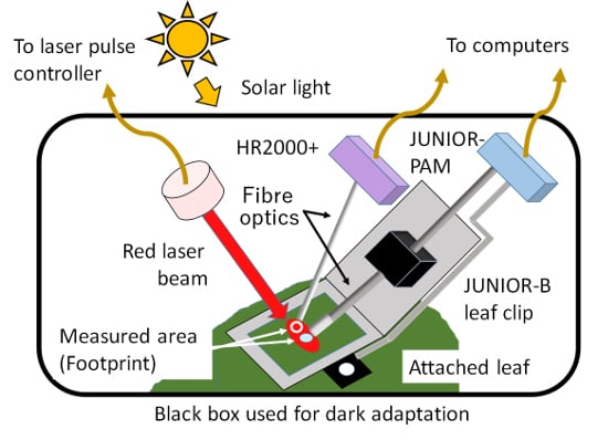
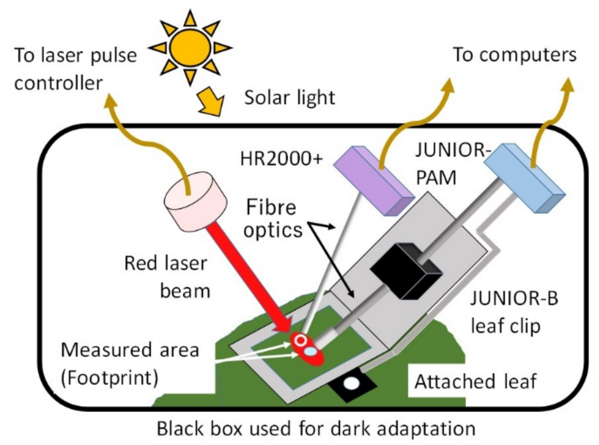
2.5. Simultaneous Measurement Using Both PAM and FLD-LISP Methods

Figure 1 shows a schematic diagram of the setup for the measurement of ChlF parameters using PAM and FLD-LISP. The experiments were carried out from 10 a.m. to 3 p.m. from August to October in an experimental room. Plants were moved from the growth chamber to the experimental room for adaptation at least one week before the experiments and were kept in the experimental room during the experiments. Air temperature in the experimental room was controlled but not recorded, however the leaf temperature was monitored by sensors attached to the JUNIOR-B leaf clip. The solar light entered through glass where its PPFD could have been variable by incident conditions via glass and cloudiness. In summer in Japan, the maximum solar light at a right-angled surface to the incident light can exceed 2000 μmol m−2 s−1, so the incident light via glass reached about 2000 μmol m−2 s−1 in this experiment. The change from dark to light was carried out by rapid movement of a black box shown in Figure 1. The focal point (measurement area, white circle on the leaf) of fibre-HR2000+ was set at a distance of 2 mm from that of the fibre-PAM (light blue filled circle) to avoid the influence of saturation pulse light and shadow of the fibre-PAM.
A time chart of the ChlF measurement using a combination of PAM and FLD-LISP methods is presented in Figure 2A. The set of sequential experiments included (i) dark adaptation of the clipped leaf area of the sample plant for 20 min; (ii) PAM measurement of maximum ChlF (Fm) during dark adaptation through switched on blue LED saturation pulse light (SLPAM); (iii) after 50 s of the PAM measurement, FLD measurement of Fm using a HR2000+ spectrometer on red laser saturation pulse light (SLRL); (iv) exposure to solar light for about 5 min; (v) PAM measurement of steady-state ChlF (Fs) and maximum ChlF (Fm’) during the light adaptation; (vi) after 20 s of the PAM measurement, FLD measurement of Fs and Fm’ using the HR2000+ spectrometer; and (vii) FLD measurement of the non-fluorescent reference (90% White Card) after about 20 s under solar light, immediately. The (v) and (vi) procedures were repeated 3 to 4 times at intervals of 40 s and it was found that the change in solar PPFD was negligible during the experiment. Several measures were taken throughout the FLD measurements to improve the Fm, Fm’, and FS retrieval accuracies. First, optimal wavelength bands were selected for the mean values of radiant intensities (Ma, Mb, Mc, and Md) (See Section 2.4 and [65]). Second, in procedures (iii) and (vi) outlined above, Fm and Fm’ were given by the mean value of three peak points during 0.6 s SLRL illumination and FS was calculated by averaging data during 10 s before the SLRL illumination using a median filter. It is known that the deviation in SIF retrieval using the FLD method is intrinsic to the method (not to the spectral resolution of the instrument, which is very high in this case) and linked to the reflectance spectral shape [67]. However, a sequence of measurements within a day would be consistent (despite the offset) since the chlorophyll content does not substantially vary and the reflectance remains mostly stable. However, there will be deviations from one date to another where the chlorophyll content has changed, thus increasing the variance and inaccuracies. Therefore, the measurements in this paper can be considered appropriate. Nevertheless, more advanced methods [68] that cope with these effects will be necessary to increase the accuracy and reliability of the SIF measurements.
After the measurement, the SPAD value (SPAD-502, Soil and Plant Analyzer Development, Konica Minolta, Tokyo, Japan) at the measured leaf area was estimated as an indicator of Chl content variations. These values were used to monitor leaf growth stages. For PPFD measurements during the experiments, an LI-250 light meter (LI-COR) and the PAM-attached sensor calibrated by LI-250 were used.

2.6. Methods for Calculating the ChlF Yield and Parameters

The ChlF yield (ΦF, the ratio of fluorescence photons to absorbed photons) was approximately calculated by
ΦF = F/(PPFD × 0.84)
where, F is the fluorescence intensity (rel. units), PPFD is the photosynthetic photon flux density (μmol m−2 s−1), and 0.84 is the leaf absorption coefficient. The ΦF can more accurately represent the relationship between the ChlF signal magnitude and PPFD than the ChlF intensity itself [2].
Then ΦPSII and NPQ were calculated by the equations below [7,9,24]:
ΦPSII = (ΦFm’ − ΦFs)/ΦFm’
where ΦFs is the steady-state ChlF yield from the light-adapted leaf (the mean value after median filtering of sequential data measured during 10 s just before the saturation laser pulse) and ΦFm’ is the saturation pulse induced ChlF yield from the light-adapted leaf.
NPQ = (ΦFm − ΦFm’)/ΦFm’
where ΦFm is the saturation pulse induced ChlF yield from the dark-adapted leaf.
ETR was estimated using the equation given by Baker (2008) [1]:
ETR = 0.5 × 0.84 × PPFD × ΦPSII

2.7. Determination of the Saturation Light Pulse Intensity

To determine the saturation pulse intensity needed for this experiment, the ChlF yields (ΦF) in paprika leaves adapted under dark and solar lights at 700 and 1300 μmol m−2 s−1 PPFD were measured at different actinic light pulse intensities using the HR2000+ system. The leaf surface was illuminated by the blue LED of JUNIOR PAM. The fibre-HR2000+ was set at a 3 mm distance from the leaf surface, and it was held at 45° to the fibre-PAM to fully detect the ChlF signal excited by the PAM actinic light. The light pulse intensities of PAM were successively raised from level 1 to 12 (25, 45, 66, 90, 125, 190, 285, 420, 625, 820, 1150, 1500 μmol m−2 s−1, respectively) at a duration of about 2 s for each intensity and an interval of 30 s. The integration time of HR2000+ was set at 0.2 s and ΦF at 760.4 nm was obtained by averaging three peak points measured during 2 s. The number of measurements was three times in 20 min dark-adapted leaves and six times in 20 min light-adapted leaves, in which measurements were done four times at about 1300 μmol m−2 s−1 and two times at about 700 μmol m−2 s−1.

3. Results

3.1. Determination of the Saturation Light Pulse Intensity

We examined the relationships between the actinic PPFDs and ChlF yields in the dark and solar light adaptation periods for paprika leaves (Figure 3) as the saturation PPFD required to saturate the photosynthetic electron transport varies with the intensity of actinic light. Figure 3A,B show the results for a dark-adapted leaf (SPAD: 47.5, measured 3 times) and solar light-adapted leaves of 700 μmol m−2 s−1 (SPAD: 48.2, measured two times: ΦF1 and ΦF2) and 1300 μmol m−2 s−1 (SPAD: 42.6, measured four times: ΦF3, ΦF4, ΦF5, and ΦF6), respectively.
The ChlF yields of the dark-adapted leaf increased dramatically with a slight increase in PPFD and levelled off approximately at a PPFD of 800 μmol m−2 s−1 (dashed line in Figure 3A). The ChlF yields of the solar light-adapted leaf increased more gradually than those of the dark-adapted leaf, leveling off approximately at a PPFD of 1800 μmol m−2 s−1 (dashed line in Figure 3B). As a result, we confirmed the saturation of the photosynthetic electron transport at PPFD values over 1800 μmol m−2 s−1 at constant solar PPFD of 1300 μmol m−2 s−1. Therefore, we decided to use the saturation pulse of the red laser that provides sufficiently strong PPFD of 6000 μmol m−2 s−1 for 0.8 s for paprika, maize, and pachira plants. This result can also be used in the PAM measurement.

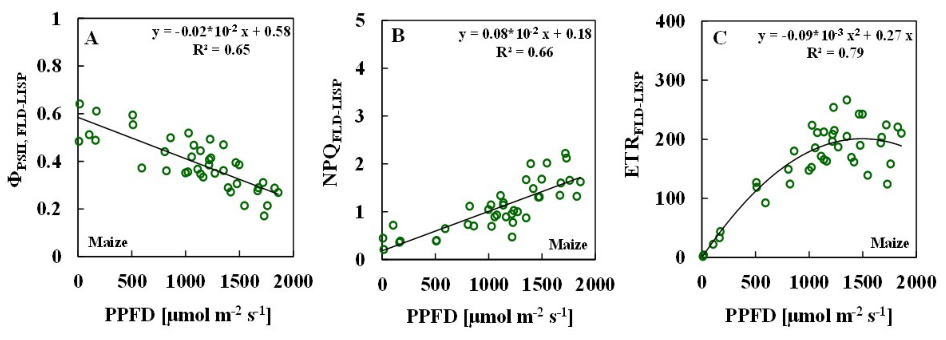
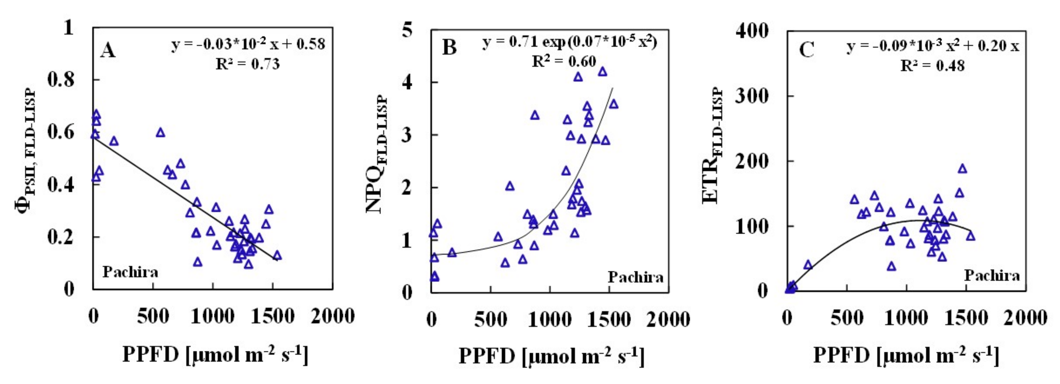
3.2. Relationships between ChlF Parameters and Solar PPFDs

We examined the relationships between the PPFD and ChlF parameters of ΦPSII, NPQ, and ETR using PAM and FLD-LISP methods for paprika, maize, and pachira plants. The details of the measurement conditions, the number of samples, SPAD values, temperature of the abaxial side of the leaf, and solar PPFD are summarized in Table 1. The experiments were performed under steady weather conditions. Figure 4, Figure 5 and Figure 6 present the results for the FLD-LISP measurements. The results of the PAM method exhibited very similar trends hence they were not presented in the plots. We also examined the relationships between SPAD values and ChlF parameters retrieved from FLD-LISP; no significant relationships were found confirming that the ChlF parameters are not affected by Chl content.
For the three plant species of paprika, maize, and pachira, the results of the relationships between ΦPSII, NPQ, and ETR and PPFDs using the FLD-LISP method are presented in Figure 4, Figure 5 and Figure 6, respectively, while the R2 values of the two methods are given in Table 1. As the solar PPFDs increased, ΦPSII decreased whereas NPQ increased exhibiting linear correlations for all three plant species, except that pachira’s NPQ was over 1000 μmol m−2 s−1 (Figure 4A,B, Figure 5A,B and Figure 6A,B, respectively). Compared to paprika, the ΦPSII and NPQ showed less variations for maize. The NPQ/PPFD relationship for pachira was non-linear, experiencing a sharp increase after the PPFD of about 1000 μmol m−2 s−1.
For ETR, increasing trends were observed when the intensities of solar light were lower than about 800 μmol m−2 s−1 for paprika (Figure 4C), lower than about 1200 μmol m−2 s−1 for maize (Figure 5C), and lower than about 800 μmol m−2 s−1 for pachira (Figure 6C). In contrast, at solar light intensities greater than that stated above, ETR showed a lot of dispersions and the regression lines began to deteriorate.

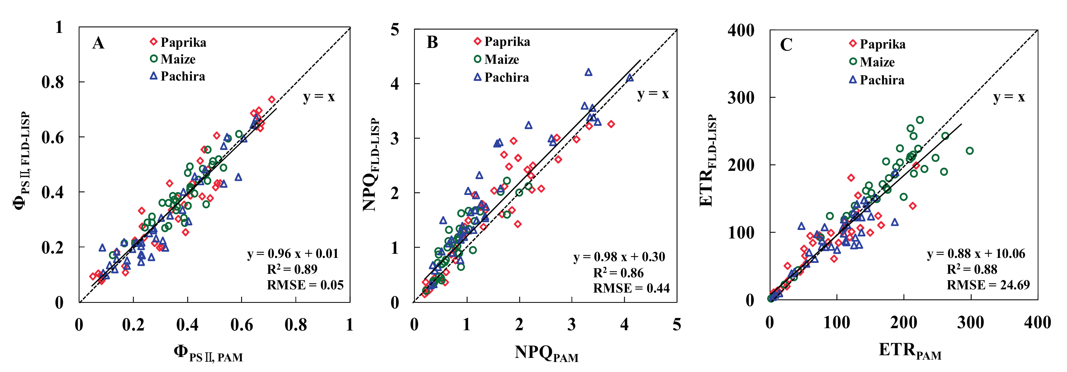
3.3. Relationships between the ChlF Parameters of the Two Methods

For the three plant species, we also examined the relationships between the ChlF parameters of ΦPSII, NPQ, and ETR determined by PAM and FLD-LISP (Figure 7). The results of each plant showed very similar trends as seen in Figure 7 and the R2 and root mean square error (RMSE) values are summarized in Table 2. The ΦPSII, NPQ, and ETR of both methods were very well correlated and the regression lines were y = 0.96x + 0.01 (R2 = 0.89, RMSE = 0.05), y = 0.98x + 0.30 (R2 = 0.86, RMSE = 0.44) and y = 0.88x + 10.06 (R2 = 0.88, RMSE = 24.69), which were approximated by y = x, although the slope for ETR was 0.88, which was smaller than 0.96 for ΦPSII, and 0.98 for NPQ. Overall, the ΦPSII of the two methods showed very small deviations for the three plant species. However, the variations of NPQ increased at higher NPQ values. In addition, the FLD-LISP NPQ estimations were slightly higher than those made by PAM.

4. Discussion

The FLD-LISP method was suggested as an effective method to measure ChlF parameters using the FLD approach. In this research, FLD-LISP was evaluated and the results were compared with ChlF parameters measured by the standard PAM method. First, the FLD-LISP ChlF yield was measured using the O2A band. To determine the saturation light pulse intensity to be used for FLD-LISP, the relationships between the actinic pulse PPFD and ChlF yields in dark-adapted and solar light-adapted paprika leaves were initially studied (Figure 3). The photosynthesis saturation PPFD of many leaves is in the range of 500–1000 μmol m−2 s−1, which is considerably lower than the direct solar PPFD of 2000 μmol m−2 s−1 [69]. Omasa et al. (2009) [18] presented that ChlF yields of the Boston fern leaf abaxial side, leaf mesophyll, and guard cell chloroplasts became constant at the saturation pulse PPFD of 800 μmol m−2 s−1 in dark-adapted conditions and 1300 μmol m−2 s−1 in light-adapted conditions. In this research a saturation pulse of >800 μmol m−2 s−1 in the dark and 1800 μmol m−2 s−1 under solar PPFD of 700 to 1300 μmol m−2 s−1 was sufficient to saturate the photosynthetic electron transport in paprika leaves (Figure 3). This is because adequately photoactivated PSII requires stronger light; the excess light energy is dissipated as heat [7,70]. The relationship between PPFD and ChlF yield at 760.4 nm using FLD-LISP confirms the results of other studies. The saturation pulse of the red laser at the PPFD of 6000 μmol m−2 s−1 for 0.8 s was used for all three plant species in this research, which is considerably larger than the photosynthesis saturation PPFDs of many leaves [69].
The FLD-LISP method was applied to measure the ChlF parameters of ΦPSII, NPQ, and ETR in three plant species, paprika (C3 plant), maize (C4 plant), and pachira (indoor C3 plant), having different carbon fixation mechanisms and light tolerance. The relationships between PPFD and FLD-LISP derived ChlF parameters of ΦPSII, NPQ, and ETR for all three plant species were studied.
In general, under high PPFD, excess light energy is dissipated as heat through the NPQ process that is regulated by the acidification of the thylakoid lumen attributed to the accumulation of protons leading to a ΔpH [4], which results in an increase in NPQ. This is an indicator of the portion of the absorbed radiation not used for electron transport in photosynthesis [4,7,71]. The regulatory protein PsbS and the conversion of violaxanthin to zeaxanthin in the xanthophyll cycle are involved in this process [4]. For both C3 and C4 plants, ΦPSII generally decreases whereas NPQ increases with increasing illumination. Also under the same level of illumination, leaves with a lower photosynthetic capacity exhibit lower ΦPSII and higher NPQ. These facts have been reported previously in various ChlF studies at leaf and cell levels [1,5,72,73,74,75,76,77,78]. The relationships between PPFD and the ChlF parameters of ΦPSII, NPQ, and ETR measured using FLD-LISP in all three plant species (Figure 4, Figure 5 and Figure 6) were similar to the relationships obtained through the PAM measurement. This confirms that the FLD-LISP method is capable of measuring ChlF parameters accurately under different PPFDs.
Both ΦPSII/PPFD and NPQ/PPFD relationships were found to be linear for paprika and maize under ordinary sunlight intensity (Figure 4A,B and Figure 5A,B). For maize, the ΦPSII values were higher and the NPQ values were lower especially in high PPFDs in comparison with paprika. These results are acceptable as paprika is a C3 plant whereas maize is a C4 plant [79,80]. For pachira, more variations were observed for NPQ when the PPFD was higher than 1000 μmol m−2 s−1. Especially, when ΦPSII decreased to smaller values, the NPQ consequently increased to a large extent (Figure 6A,B). These results are expected because pachira is an indoor C3 plant adapted to low light. The ETR/PPFD relationship was nonlinear in all plants. The maximum ETR for maize was about twice as that for paprika and pachira. Increasing trends were observed for PPFD values lower than about 800 μmol m−2 s−1 for paprika and pachira (Figure 4C and Figure 6C) and lower than about 1200 μmol m−2 s−1 for maize (Figure 5C), but the ETR decreased at high PPFD. This phenomenon may be caused by photoinhibition under high solar light because the plant materials were cultured at low PPFD under fluorescent and LED lights. Some of the variations seen in Figure 4, Figure 5 and Figure 6 might have also been related to the effects of temperature and other environmental conditions.
Finally, ChlF parameters measured in different growth stages and light conditions using FLD-LISP and PAM were compared. The ΦPSII, NPQ, and ETR of both methods were very well correlated confirming good accuracy of FLD-LISP to estimate ChlF parameters regardless of differences in plant growth stages (variable Chl content) and in the response of the species to light. The ΦPSII of the two methods were better correlated compared to NPQ (Figure 7A,B). NPQ values derived from FLD-LISP were slightly higher than those obtained from PAM. This can be related to the difference in the method used for ΦFm and ΦFm’ measurements (see Materials and Methods section). The variations of ETR increased at higher ETR values and the slope of regression equation was 0.88 for ETR (Figure 7C). This may have been caused by differences in light calibration between FLD-LISP and PAM.
The results presented in this research confirm the capability of FLD-LISP to measure ChlF parameters and the photosynthesis capacity of plants. The potential sources of error using this method as described by Tubuxin et al. (2015) [65] can be (i) noise in the spectrometer; (ii) solar light fluctuations including incident light variations through the glass during the measurement; (iii) differences in the angle of the uneven leaf surface and non-fluorescent reference; and (iv) the inaccuracy of the PPFD measurement on the leaf. In addition, variations in temperature and environmental conditions may affect the accuracy of the measurements. These sources of error need to be considered for the future applications of the suggested methodology. Several measures were taken in this research to improve the FLD method and to increase the ChlF retrieval accuracy. The results indicated that the applied measures were effective as good relationships were observed between the ChlF parameters measured using FLD-LISP and those retrieved from PAM, provided that they were measured simultaneously within a short time frame. At the same time, the presence of samples with a range of chlorophyll content might have resulted in an increased variance in the results due to the limitations of the standard FLD method. However, techniques such as improved FLD (iFLD) or spectral fitting [67,68,81] can be other improved alternatives for the FLD retrieval and are recommended to be evaluated and used in future applications of the developed FLD-LISP method.

5. Conclusions

To address the shortcomings of the SIF method, including the inability to measure the ChlF parameters and being affected by the plant’s Chl content, we have introduced a new technique using a joint Fraunhofer line depth and laser induced saturation pulse method (FLD-LISP) to measure photosynthesis signals directly [65]. In this paper a more comprehensive study of FLD-LISP was presented to better evaluate the performance of the suggested methodology for the measurement of ChlF parameters. We evaluated the performance of FLD-LISP to measure ΦPSII, NPQ, and ETR under different actinic PPFDs in three C3 and C4 plant species having different responses to light. The PAM method was used to verify and understand the FLD-LISP. The effect of PPFD on ΦPSII, NPQ, and ETR exhibited the same trend regardless of the method used to estimate ChlF parameters in all three plant species. The ΦPSII, NPQ, and ETR values derived using FLD-LISP and PAM were very well correlated, confirming the good accuracy of FLD-LISP to estimate ChlF parameters regardless of growth stages (variable Chl content) and differences in species confirming the usefulness of FLD-LISP to measure ChlF parameters and plant photosynthesis activity.
Finally, the FLD-LISP method does not need accurate pulse-synchronized and modulated fluorimetric techniques as the PAM and LIFT methods do. For long-distance (canopy scale) measurement of ChlF parameters using FLD-LISP, the combination of FLD-LISP and LIFT’s lighting technique, which is interpolated to a maximum fluorescence level using a series of low-intensity laser pulses and a fluorescence model, would be recommended.

Acknowledgments

This work was supported by the Japan Society for the Promotion of Science (Grant No. 24248043).

Author Contributions

Kenji Omasa (K.O.), Parinaz Rahimzadeh-Bajgiran (P.R.-B.) and Bayaer Tubuxin (B.T.) conceived and designed the experiments; B.T and K.O. performed the experiments and analyzed the data; P.R.-B., B.T., and K.O wrote the paper and discussed the results.

Conflicts of Interest

The authors declare no conflict of interest.

References

  1. Baker, N.R. Chlorophyll fluorescence: A probe of photosynthesis in vivo. Annu. Rev. Plant Biol. 2008, 59, 89–113. [Google Scholar] [CrossRef] [PubMed]
  2. Govindjee. 63 years since kautsky—Chlorophyll-a fluorescence. Aust. J. Plant Physiol. 1995, 22, 131–160. [Google Scholar]
  3. Kautsky, H.; Hirsch, A. Neue versuche zur kohlensäureassimilation. Naturwissenschaften 1931, 19, 964. [Google Scholar] [CrossRef]
  4. Murchie, E.H.; Lawson, T. Chlorophyll fluorescence analysis: A guide to good practice and understanding some new applications. J. Exp. Bot. 2013, 64, 3983–3998. [Google Scholar] [CrossRef] [PubMed]
  5. Papageorgiou, G.C.; Govindjee. Chlorophyll a Fluorescence: A Signature of Photosynthesis; Springer: Dordrecht, The Netherlands, 2004; Volume 19. [Google Scholar]
  6. Porcar-Castell, A.; Tyystjarvi, E.; Atherton, J.; Van der Tol, C.; Flexas, J.; Pfundel, E.E.; Moreno, J.; Frankenberg, C.; Berry, J.A. Linking chlorophyll a fluorescence to photosynthesis for remote sensing applications: Mechanisms and challenges. J. Exp. Bot. 2014, 65, 4065–4095. [Google Scholar] [CrossRef] [PubMed]
  7. Bilger, W.; Bjorkman, O. Role of the xanthophyll cycle in photoprotection elucidated by measurement of light-induced absorbency changes, fluorescence and photosynthesis in leaves of Hedera canariensis. Photosynth. Res. 1990, 25, 173–185. [Google Scholar] [CrossRef] [PubMed]
  8. Buschmann, C.; Nagel, E.; Szabo, K.; Kocsanyi, L. Spectrometer for fast measurements of in vivo reflectance, absorption and fluorescence in the visible and near-infrared. Remote Sens. Environ. 1994, 48, 18–24. [Google Scholar] [CrossRef]
  9. Genty, B.; Briantais, J.M.; Baker, N.R. The relationship between the quantum yield of photosynthetic electron-transport and quenching of chlorophyll fluorescence. Biochim. Biophys. Acta 1989, 990, 87–92. [Google Scholar] [CrossRef]
  10. Lichtenthaler, H.K.; Buschmann, C.; Rinderle, U.; Schmuck, G. Application of chlorophyll fluorescence in ecophysiology. Radiat. Environ. Biophys. 1986, 25, 297–308. [Google Scholar] [CrossRef] [PubMed]
  11. Lichtenthaler, H.K.; Rinderle, U. The role of chlorophyll fluorescence in the detection of stress conditions in plants. CRC Crit. Rev. Anal. Chem. 1988, 19, S29–S85. [Google Scholar] [CrossRef]
  12. Schreiber, U.; Schliwa, U.; Bilger, W. Continuous recording of photochemical and non-photochemical chlorophyll fluorescence quenching withe a new type of modulation fluorometer. Photosynth. Res. 1986, 10, 51–62. [Google Scholar] [CrossRef] [PubMed]
  13. Daley, P.F.; Raschke, K.; Ball, J.T.; Berry, J.A. Topography of photosynthetic activity of leaves obtained from video imaged of chlorophyll fluorescence. Plant Physiol. 1989, 90, 1233–1238. [Google Scholar] [CrossRef] [PubMed]
  14. Genty, B.; Meyer, S. Quantitative mapping of leaf photosynthesis using chlorophyll fluorescence imaging. Aust. J. Plant Physiol. 1995, 22, 277–284. [Google Scholar] [CrossRef]
  15. Govindjee; Nedbal, G.L. Seeing is believing. Photosynthetica 2000, 38, 481–482. [Google Scholar]
  16. Lichtenthaler, H.K.; Lang, M.; Sowinska, M.; Heisel, F.; Miehe, J.A. Detection of vegetation stress via a new high resolution fluorescence imaging system. J. Plant Physiol. 1996, 148, 599–612. [Google Scholar] [CrossRef]
  17. Omasa, K.; Hosoi, F.; Konishi, A. 3D lidar imaging for detecting and understanding plant responses and canopy structure. J. Exp. Bot. 2007, 58, 881–898. [Google Scholar] [CrossRef] [PubMed]
  18. Omasa, K.; Konishi, A.; Tamura, H.; Hosoi, F. 3D confocal laser scanning microscopy for the analysis of chlorophyll fluorescence parameters of chloroplasts in intact leaf tissues. Plant Cell Physiol. 2009, 50, 90–105. [Google Scholar] [CrossRef] [PubMed]
  19. Omasa, K.; Shimazaki, K.I.; Aiga, I.; Larcher, W.; Onoe, M. Image analysis of chlorophyll fluorescence transients for diagnosing the photosynthetic system of attached leaves. Plant Physiol. 1987, 84, 748–752. [Google Scholar] [CrossRef] [PubMed]
  20. Omasa, K.; Takayama, K. Simultaneous measurement of stomatal conductance, non-photochemical quenching, and photochemical yield of photosystem ii in intact leaves by thermal and chlorophyll fluorescence imaging. Plant Cell Physiol. 2003, 44, 1290–1300. [Google Scholar] [CrossRef] [PubMed]
  21. Osmond, B.; Park, Y. Field-portable imaging system for measurement of chlorophyll fluorescence quenching. In Air Pollution and Plant Biotechnology; Springer: Tokyo, Japan, 2002; pp. 309–319. [Google Scholar]
  22. Oxborough, K. Imaging of chlorophyll a fluorescence: Theoretical and practical aspects of an emerging technique for the monitoring of photosynthetic performance. J. Exp. Bot. 2004, 55, 1195–1205. [Google Scholar] [CrossRef] [PubMed]
  23. Schreiber, U. Pulse-amplitude-modulation (PAM) fluorometry and saturation pulse method: An overview. In Chlorophyll a Fluorescence. A Signature of Photosynthesis; Papageorgiou, G.C., Govindgee, Eds.; Springer: Dordrecht, The Netherlands, 2004; pp. 279–319. [Google Scholar]
  24. Maxwell, K.; Johnson, G.N. Chlorophyll fluorescence—A practical guide. J. Exp. Bot. 2000, 51, 659–668. [Google Scholar] [CrossRef] [PubMed]
  25. Govender, M.; Dye, P.J.; Weiersbye, I.M.; Witkowski, E.T.F.; Ahmed, F. Review of commonly used remote sensing and ground-based technologies to measure plant water stress. Water SA 2009, 35, 741–752. [Google Scholar] [CrossRef]
  26. Grace, J.; Nichol, C.; Disney, M.; Lewis, P.; Quaife, T.; Bowyer, P. Can we measure terrestrial photosynthesis from space directly, using spectral reflectance and fluorescence? Glob. Chang. Biol. 2007, 13, 1484–1497. [Google Scholar] [CrossRef]
  27. Meroni, M.; Rossini, M.; Guanter, L.; Alonso, L.; Rascher, U.; Colombo, R.; Moreno, J. Remote sensing of solar-induced chlorophyll fluorescence: Review of methods and applications. Remote Sens. Environ. 2009, 113, 2037–2051. [Google Scholar] [CrossRef]
  28. Corp, L.A.; McMurtrey, J.E.; Middleton, E.M.; Mulchi, C.L.; Chappelle, E.W.; Daughtry, C.S.T. Fluorescence sensing systems: In vivo detection of biophysical variations in field corn due to nitrogen supply. Remote Sens. Environ. 2003, 86, 470–479. [Google Scholar] [CrossRef]
  29. Konishi, A.; Eguchi, A.; Hosoi, F.; Omasa, K. 3D monitoring spatio-temporal effects of herbicide on a whole plant using combined range and chlorophyll a fluorescence imaging. Funct. Plant Biol. 2009, 36, 874–879. [Google Scholar] [CrossRef]
  30. Lichtenthaler, H.K. Vegetation stress: An introduction to the stress concept in plants. J. Plant Physiol. 1996, 148, 4–14. [Google Scholar] [CrossRef]
  31. Lichtenthaler, H.K.; Miehe, J.A. Fluorescence imaging as a diagnostic tool for plant stress. Trends Plant Sci. 1997, 2, 316–320. [Google Scholar] [CrossRef]
  32. Schächtl, J.; Huber, G.; Maidl, F.-X.; Sticksel, E.; Schulz, J.; Haschberger, P. Laser-induced chlorophyll fluorescence measurements for detecting the nitrogen status of wheat (triticum aestivum L.) canopies. Precis. Agric. 2005, 6, 143–156. [Google Scholar] [CrossRef]
  33. Sun, Y.; Fu, R.; Dickinson, R.; Joiner, J.; Frankenberg, C.; Gu, L.H.; Xia, Y.L.; Fernando, N. Drought onset mechanisms revealed by satellite solar-induced chlorophyll fluorescence: Insights from two contrasting extreme events. J. Geophys. Res. Biogeosci. 2015, 120, 2427–2440. [Google Scholar] [CrossRef]
  34. Zarco-Tejada, P.J.; Gonzalez-Dugo, V.; Berni, J.A.J. Fluorescence, temperature and narrow-band indices acquired from a UAV platform for water stress detection using a micro-hyperspectral imager and a thermal camera. Remote Sens. Environ. 2012, 117, 322–337. [Google Scholar] [CrossRef]
  35. Omasa, K. Image instrumentation of chlorophyll a fluorescence. In Advances in Laser Remote Sensing for Terrestrial and Hydrographic Applications, Proceedings of the SPIE 3382, Orlando, FL, USA, 13 April 1998; Narayanan, R.M., Kalshoven, J.E., Jr., Eds.; SPIE: Bellingham, WA, USA, 1998; pp. 91–98. [Google Scholar]
  36. Kolber, Z.; Klimov, D.; Ananyev, G.; Rascher, U.; Berry, J.; Osmond, B. Measuring photosynthetic parameters at a distance: Laser induced fluorescence transient (lift) method for remote measurements of photosynthesis in terrestrial vegetation. Photosynth. Res. 2005, 84, 121–129. [Google Scholar] [CrossRef] [PubMed]
  37. Kolber, Z.S.; Prasil, O.; Falkowski, P.G. Measurements of variable chlorophyll fluorescence using fast repetition rate techniques: Defining methodology and experimental protocols. Biochim. Biophys. Acta Bioenerg. 1998, 1367, 88–106. [Google Scholar] [CrossRef]
  38. Pieruschka, R.; Albrecht, H.; Muller, O.; Berry, J.A.; Klimov, D.; Kolber, Z.S.; Malenovsky, Z.; Rascher, U. Daily and seasonal dynamics of remotely sensed photosynthetic efficiency in tree canopies. Tree Physiol. 2014, 34, 674–685. [Google Scholar] [CrossRef] [PubMed]
  39. Pieruschka, R.; Klimov, D.; Berry, J.A.; Osmond, C.B.; Rascher, U.; Kolber, Z.S. Remote chlorophyll fluorescence measurements with the laser-induced fluorescence transient approach. In High-Throughput Phenotyping in Plants: Methods and Protocols; Normanly, J., Ed.; Humana Press: New York, NY, USA, 2012; pp. 51–59. [Google Scholar]
  40. Plascyk, J.A.; Gabriel, F.C. The fraunhofer line discriminator mk ii—An airborne instrument for precise and standardized ecological luminescence measurement. IEEE Trans. Instrum. Meas. 1975, 24, 306–313. [Google Scholar] [CrossRef]
  41. Joiner, J.; Guanter, L.; Lindstrot, R.; Voigt, M.; Vasilkov, A.P.; Middleton, E.M.; Huemmrich, K.F.; Yoshida, Y.; Frankenberg, C. Global monitoring of terrestrial chlorophyll fluorescence from moderate-spectral-resolution near-infrared satellite measurements: Methodology, simulations, and application to GOME-2. Atmos. Meas. Tech. 2013, 6, 2803–2823. [Google Scholar] [CrossRef]
  42. Cogliati, S.; Rossini, M.; Julitta, T.; Meroni, M.; Schickling, A.; Burkart, A.; Pinto, F.; Rascher, U.; Colombo, R. Continuous and long-term measurements of reflectance and sun-induced chlorophyll fluorescence by using novel automated field spectroscopy systems. Remote Sens. Environ. 2015, 164, 270–281. [Google Scholar] [CrossRef]
  43. Corp, L.A.; Middleton, E.M.; McMurtrey, J.E.; Campbell, P.K.E.; Butcher, L.M. Fluorescence sensing techniques for vegetation assessment. Appl. Opt. 2006, 45, 1023–1033. [Google Scholar] [CrossRef] [PubMed]
  44. Julitta, T.; Corp, L.A.; Rossini, M.; Burkart, A.; Cogliati, S.; Davies, N.; Hom, M.; Mac Arthur, A.; Middleton, E.M.; Rascher, U.; et al. Comparison of sun-induced chlorophyll fluorescence estimates obtained from four portable field spectroradiometers. Remote Sens. 2016, 8, 122. [Google Scholar] [CrossRef]
  45. Liu, L.Y.; Zhang, Y.J.; Wang, J.H.; Zhao, C.J. Detecting solar-induced chlorophyll fluorescence from field radiance spectra based on the fraunhofer line principle. IEEE Trans. Geosci. Remote Sens. 2005, 43, 827–832. [Google Scholar]
  46. Moya, I.; Camenen, L.; Evain, S.; Goulas, Y.; Cerovic, Z.G.; Latouche, G.; Flexas, J.; Ounis, A. A new instrument for passive remote sensing 1. Measurements of sunlight-induced chlorophyll fluorescence. Remote Sens. Environ. 2004, 91, 186–197. [Google Scholar] [CrossRef]
  47. Rascher, U.; Agati, G.; Alonso, L.; Cecchi, G.; Champagne, S.; Colombo, R.; Damm, A.; Daumard, F.; De Miguel, E.; Fernandez, G.; et al. Cefles2: The remote sensing component to quantify photosynthetic efficiency from the leaf to the region by measuring sun-induced fluorescence in the oxygen absorption bands. Biogeosciences 2009, 6, 1181–1198. [Google Scholar] [CrossRef]
  48. Rascher, U.; Alonso, L.; Burkart, A.; Cilia, C.; Cogliati, S.; Colombo, R.; Damm, A.; Drusch, M.; Guanter, L.; Hanus, J.; et al. Sun-induced fluorescence—A new probe of photosynthesis: First maps from the imaging spectrometer hyplant. Glob. Chang. Biol. 2015, 21, 4673–4684. [Google Scholar] [CrossRef] [PubMed]
  49. Rossini, M.; Meroni, M.; Celesti, M.; Cogliati, S.; Julitta, T.; Panigada, C.; Rascher, U.; Van der Tol, C.; Colombo, R. Analysis of red and far-red sun-induced chlorophyll fluorescence and their ratio in different canopies based on observed and modeled data. Remote Sens. 2016, 8, 412. [Google Scholar] [CrossRef]
  50. Rossini, M.; Panigada, C.; Cilia, C.; Meroni, M.; Busetto, L.; Cogliati, S.; Amaducci, S.; Colombo, R. Discriminating irrigated and rainfed maize with diurnal fluorescence and canopy temperature airborne maps. ISPRS Int. J. Geo-Inf. 2015, 4, 626–646. [Google Scholar] [CrossRef]
  51. Zarco-Tejada, P.J.; Berni, J.A.J.; Suarez, L.; Sepulcre-Canto, G.; Morales, F.; Miller, J.R. Imaging chlorophyll fluorescence with an airborne narrow-band multispectral camera for vegetation stress detection. Remote Sens. Environ. 2009, 113, 1262–1275. [Google Scholar] [CrossRef]
  52. Hilker, T.; Coops, N.C.; Wulder, M.A.; Black, T.A.; Guy, R.D. The use of remote sensing in light use efficiency based models of gross primary production: A review of current status and future requirements. Sci. Total Environ. 2008, 404, 411–423. [Google Scholar] [CrossRef] [PubMed]
  53. Frankenberg, C.; Fisher, J.B.; Worden, J.; Badgley, G.; Saatchi, S.S.; Lee, J.E.; Toon, G.C.; Butz, A.; Jung, M.; Kuze, A.; et al. New global observations of the terrestrial carbon cycle from gosat: Patterns of plant fluorescence with gross primary productivity. Geophys. Res. Lett. 2011, 38, 351–365. [Google Scholar] [CrossRef]
  54. Guanter, L.; Zhang, Y.G.; Jung, M.; Joiner, J.; Voigt, M.; Berry, J.A.; Frankenberg, C.; Huete, A.R.; Zarco-Tejada, P.; Lee, J.E.; et al. Global and time-resolved monitoring of crop photosynthesis with chlorophyll fluorescence. Proc. Natl. Acad. Sci. USA 2014, 111, E1327–E1333. [Google Scholar] [CrossRef] [PubMed]
  55. Joiner, J.; Yoshida, Y.; Vasilkov, A.P.; Yoshida, Y.; Corp, L.A.; Middleton, E.M. First observations of global and seasonal terrestrial chlorophyll fluorescence from space. Biogeosciences 2011, 8, 637–651. [Google Scholar] [CrossRef]
  56. Kohler, P.; Guanter, L.; Frankenberg, C. Simplified physically based retrieval of sun-induced chlorophyll fluorescence from gosat data. IEEE Geosci. Remote Sens. Lett. 2015, 12, 1446–1450. [Google Scholar] [CrossRef]
  57. Koffi, E.N.; Rayner, P.J.; Norton, A.J.; Frankenberg, C.; Scholze, M. Investigating the usefulness of satellite-derived fluorescence data in inferring gross primary productivity within the carbon cycle data assimilation system. Biogeosciences 2015, 12, 4067–4084. [Google Scholar] [CrossRef]
  58. Liu, L.Y.; Guan, L.; Liu, X. Directly estimating diurnal changes in GPP for C3 and C4 crops using far-red sun-induced chlorophyll fluorescence. Agric. For. Meteorol. 2017, 232, 1–9. [Google Scholar] [CrossRef]
  59. Wagle, P.; Zhang, Y.G.; Jin, C.; Xiao, X.M. Comparison of solar-induced chlorophyll fluorescence, light-use efficiency, and process-based GPP models in maize. Ecol. Appl. 2016, 26, 1211–1222. [Google Scholar] [CrossRef] [PubMed]
  60. Yang, X.; Tang, J.W.; Mustard, J.F.; Lee, J.E.; Rossini, M.; Joiner, J.; Munger, J.W.; Kornfeld, A.; Richardson, A.D. Solar-induced chlorophyll fluorescence that correlates with canopy photosynthesis on diurnal and seasonal scales in a temperate deciduous forest. Geophys. Res. Lett. 2015, 42, 2977–2987. [Google Scholar] [CrossRef]
  61. Van der Tol, C.; Berry, J.A.; Campbell, P.K.E.; Rascher, U. Models of fluorescence and photosynthesis for interpreting measurements of solar-induced chlorophyll fluorescence. J. Geophys. Res. Biogeosci. 2014, 119, 2312–2327. [Google Scholar] [CrossRef] [PubMed]
  62. Verrelst, J.; Van der Tol, C.; Magnani, F.; Sabater, N.; Rivera, J.P.; Mohammed, G.; Moreno, J. Evaluating the predictive power of sun-induced chlorophyll fluorescence to estimate net photosynthesis of vegetation canopies: A scope modeling study. Remote Sens. Environ. 2016, 176, 139–151. [Google Scholar] [CrossRef]
  63. Zarco-Tejada, P.J.; Gonzalez-Dugo, M.V.; Fereres, E. Seasonal stability of chlorophyll fluorescence quantified from airborne hyperspectral imagery as an indicator of net photosynthesis in the context of precision agriculture. Remote Sens. Environ. 2016, 179, 89–103. [Google Scholar] [CrossRef]
  64. Kraft, S.; Bezy, J.L.; Del Bello, U.; Berlich, R.; Drusch, M.; Franco, R.; Gabriele, A.; Harnisch, B.; Meynart, R.; Silvestrin, P. FLORIS: Phase A status of the fluorescence imaging spectrometer of the earth explorer mission candidate FLEX. In Proceedings of SPIE 8889, Dresden, Germany, 23 September 2013; Sensors, Systems, and Next-Generation Satellites XVII; Meynart, R., Neeck, S.P., Shimoda, H., Eds.; SPIE: Bellingham, WA, USA, 2013; p. 88890T. [Google Scholar]
  65. Tubuxin, B.; Rahimzadeh-Bajgiran, P.; Ginnan, Y.; Hosoi, F.; Omasa, K. Estimating chlorophyll content and photochemical yield of photosystem ii (φpsii) using solar-induced chlorophyll fluorescence measurements at different growing stages of attached leaves. J. Exp. Bot. 2015, 66, 5595–5603. [Google Scholar] [CrossRef] [PubMed]
  66. Cendrero-Mateo, M.P.; Moran, M.S.; Papuga, S.A.; Thorp, K.R.; Alonso, L.; Moreno, J.; Ponce-Campos, G.; Rascher, U.; Wang, G. Plant chlorophyll fluorescence: Active and passive measurements at canopy and leaf scales with different nitrogen treatments. J. Exp. Bot. 2016, 67, 275–286. [Google Scholar] [CrossRef] [PubMed]
  67. Alonso, L.; Gomez-Chova, L.; Vila-Frances, J.; Amoros-Lopez, J.; Guanter, L.; Calpe, J.; Moreno, J. Improved Fraunhofer Line Discrimination Method for Vegetation Fluorescence Quantification. IEEE Geosci. Remote Sens. Lett. 2008, 5, 620–624. [Google Scholar] [CrossRef]
  68. Damm, A.; Erler, A.; Hillen, W.; Meroni, M.; Schaepman, M.E.; Verhoef, W.; Rascher, U. Modeling the impact of spectral sensor configurations on the FLD retrieval accuracy of sun-induced chlorophyll fluorescence. Remote Sens. Environ. 2011, 115, 1882–1892. [Google Scholar] [CrossRef]
  69. Taiz, L.; Zeiger, E. Plant Physiology; Sinauer Associates Inc.: Sunderland, MA, USA, 2002. [Google Scholar]
  70. Noctor, G.; Horton, P. Uncoupler titration of energy-dependent chlorophyll fluorescence quenching and photosystem ii photochemical yield in intact pea chloroplasts. Biochim. Biophys. Acta 1990, 1016, 228–234. [Google Scholar] [CrossRef]
  71. Demmig-Adams, B.; Adams, W.W. Photoprotection and other responses of plants to high light stress. Annu. Rev. Plant Physiol. Plant Mol. Biol. 1992, 43, 599–626. [Google Scholar] [CrossRef]
  72. Demmig, B.; Bjorkman, O. Comparison of the effect of excessive light on chlorophyll fluorescence (77k) and photon yield of O2 evolution in leaves of higher plants. Planta 1987, 171, 171–184. [Google Scholar] [CrossRef] [PubMed]
  73. Demmig-Adams, B.; Adams, W.W.; Barker, D.H.; Logan, B.A.; Bowling, D.R.; Verhoeven, A.S. Using chlorophyll fluorescence to assess the fraction of absorbed light allocated to thermal dissipation of excess excitation. Physiol. Plant. 1996, 98, 253–264. [Google Scholar] [CrossRef]
  74. Goh, C.H.; Schreiber, U.; Hedrich, R. New approach of monitoring changes in chlorophyll a fluorescence of single guard cells and protoplasts in response to physiological stimuli. Plant Cell Environ. 1999, 22, 1057–1070. [Google Scholar] [CrossRef]
  75. Kato, M.C.; Hikosaka, K.; Hirotsu, N.; Makino, A.; Hirose, T. The excess light energy that is neither utilized in photosynthesis nor dissipated by photoprotective mechanisms determines the rate of photoinactivation in photosystem ii. Plant Cell Physiol. 2003, 44, 318–325. [Google Scholar] [CrossRef] [PubMed]
  76. Lawson, T.; Oxborough, K.; Morison, J.I.L.; Baker, N.R. Responses of photosynthetic electron transport in stomatal guard cells and mesophyll cells in intact leaves to light, CO2, and humidity. Plant Physiol. 2002, 128, 52–62. [Google Scholar] [CrossRef] [PubMed]
  77. Lawson, T.; Oxborough, K.; Morison, J.I.L.; Baker, N.R. The responses of guard and mesophyll cell photosynthesis to CO2, O2, light, and water stress in a range of species are similar. J. Exp. Bot. 2003, 54, 1743–1752. [Google Scholar] [CrossRef] [PubMed]
  78. Oliveira, G.; Penuelas, J. Allocation of absorbed light energy into photochemistry and dissipation in a semi-deciduous and an evergreen mediterranean woody species during winter. Aust. J. Plant Physiol. 2001, 28, 471–480. [Google Scholar]
  79. Krall, J.P.; Edwards, G.E.; Ku, M.S.B. Quantum yield of photosystem-II and efficiency of CO2 fixation in flaveria (asteraceae) species under varying light and CO2. Aust. J. Plant Physiol. 1991, 18, 369–383. [Google Scholar] [CrossRef]
  80. Peterson, R.B. Regulation of electron-transport in photosystem-I and photosystem-Ii in C3, C3-C4, and C4 species of panicum in response to changing irradiance and O2 levels. Plant Physiol. 1994, 105, 349–356. [Google Scholar] [CrossRef] [PubMed]
  81. Cogliati, S.; Verhoef, W.; Kraft, S.; Sabater, N.; Alonso, L.; Vicent, J.; Moreno, J.; Drusch, M.; Colombo, R. Retrieval of sun-induced fluorescence using advanced spectral fitting methods. Remote Sens. Environ. 2015, 169, 344–357. [Google Scholar] [CrossRef]
Figure 1. Schematic diagram for the measurement of ChlF (Chlorophyll Fluorescence) parameters using PAM (Pulse Amplitude-Modulated) and FLD-LISP (Fraunhofer Line Depth and Laser-Induced Saturation Pulse) methods. The focal point (measurement area, white circle on leaf) of fibre-HR2000+ was set at a distance of 2 mm from that of the fibre-PAM (light blue filled circle) to avoid the influence of saturation pulse light and shadow of the fibre-PAM. Red filled area on the leaf is the footprint of the red laser beam. A black box was used to switch between dark condition and solar light. The timing and duty ratio of the red laser radiation were maintained by a laser pulse controller.
Remotesensing 09 00599 g001
Figure 2. Typical measurement diagrams of ChlF parameters using PAM and FLD-LISP. (A) a time sequence of lighting for leaf radiance spectral measurements using a HR2000+ spectrometer and PAM measurement during the dark and solar light adaptation periods. SLRL is the saturation light pulse (PPFD, Photosynthetic Photon Flux Density): 6000 μmol m−2 s−1) using a red laser (660 nm) for measurement using HR2000+ and SLPAM is the saturation light pulse (blue LED, PPFD about 10,000 μmol m−2 s−1) for measurement using JUNIOR PAM (Heinz Walz GmbH, Effeltrich. Germany); (B) temporal changes in ChlF yield (ΦF: near 760.4 nm) estimated by FLD-LISP, where ΦFm and ΦFm’ are the laser saturation pulse-induced ChlF yields in dark-adapted and light-adapted leaves, respectively. The thick line is the mean value after median filtering during 10 s before the SLRL illumination for estimating the steady-state ChlF yield (ΦFs).
Remotesensing 09 00599 g002
Figure 3. Relationships between light pulse PPFD and ChlF yield (ΦF: near 760.4 nm) of paprika leaves. (A) results in the dark-adapted leaf (SPAD value of 47.5, measured by SPAD-502, Soil and Plant Analyzer Development, Konica Minolta, Tokyo, Japan) measured three times (ΦF1 to ΦF3); (B) results in the light-adapted leaf (SPAD value of 42.6) measured twice (ΦF1 and ΦF2) at solar PPFD of 700 μmol m−2 s−1 and four times (ΦF3 to ΦF6) at 1300 μmol m−2 s−1. The JUNIOR PAM actinic light system was used as the light pulse source. Dashed lines represent the minimal PPFD for the saturation light pulse.
Remotesensing 09 00599 g003
Figure 4. Relationships between solar PPFD and ChlF parameters (A) ΦPSII; (B) NPQ; and (C) ETR of paprika leaves estimated by the FLD-LISP method. The results of the PAM method were very similar and the details are given in Table 1.
Remotesensing 09 00599 g004
Figure 5. Relationships between the solar PPFD and the ChlF parameters (A) ΦPSII; (B) NPQ; and (C) ETR of maize leaves estimated by the FLD-LISP method. The results of the PAM method were very similar and the details are given in Table 1.
Remotesensing 09 00599 g005
Figure 6. Relationships between the solar PPFD and ChlF parameters (A) ΦPSII; (B) NPQ; and (C) ETR of pachira leaves estimated by the FLD-LISP method. The results of the PAM method were very similar and the details are given in Table 1.
Remotesensing 09 00599 g006
Figure 7. Relationships between the ChlF parameters estimated by the two methods (PAM and FLD-LISP) (A) ΦPSII; (B) NPQ; and (C) ETR. The diamonds, circles, and triangles represent the results of paprika, maize, and pachira, respectively. R2 and RMSE of all samples are shown in the figures and the results are summarized in Table 2.
Remotesensing 09 00599 g007
Table 1. Experimental conditions of the three plant species and the coefficients of determination (R2) between ChlF parameters (ΦPSII, photochemical yield of photosystem II; NPQ, non-photochemical quenching; and ETR, photosystem II-based electron transport rate) and solar PPFD using the PAM and FLD-LISP methods.
Measurement MethodsNumber of SamplesSPADTemperature (°C)Solar Light
PPFD (µmol m−2 s−1)
R2
ɸPSII/PPFD
R2
NPQ/PPFD
R2
ETR/PPFD
Paprika3937.5–52.920.8–35.211–1726
PAM0.740.690.55
FLD-LISP0.760.690.59
Maize4022.7–36.621.1–32.79–1860
PAM0.580.430.71
FLD-LISP0.650.660.79
Pachira4023.2–56.120.1–27.617–1537
PAM0.750.540.46
FLD-LISP0.730.600.48
Table 2. Coefficients of determination (R2) and RMSE between the ChlF parameters (ΦPSII, NPQ, and ETR) measured by the PAM and FLD-LISP methods for the three plant species. This table is a summary of Figure 7.
MaterialsɸPSIINPQETR
R2RMSER2RMSER2RMSE
Paprika0.900.060.850.400.8124.82
Maize0.840.050.780.340.8725.80
Pachira0.900.060.880.560.7923.38
Total0.890.050.860.440.8824.69

