
Intercomparison of Ozone Vertical Profile Measurements by Differential Absorption Lidar and IASI/MetOp Satellite in the Upper Troposphere–Lower Stratosphere

 , and
, and
Abstract
:
1. Introduction
2. Methods
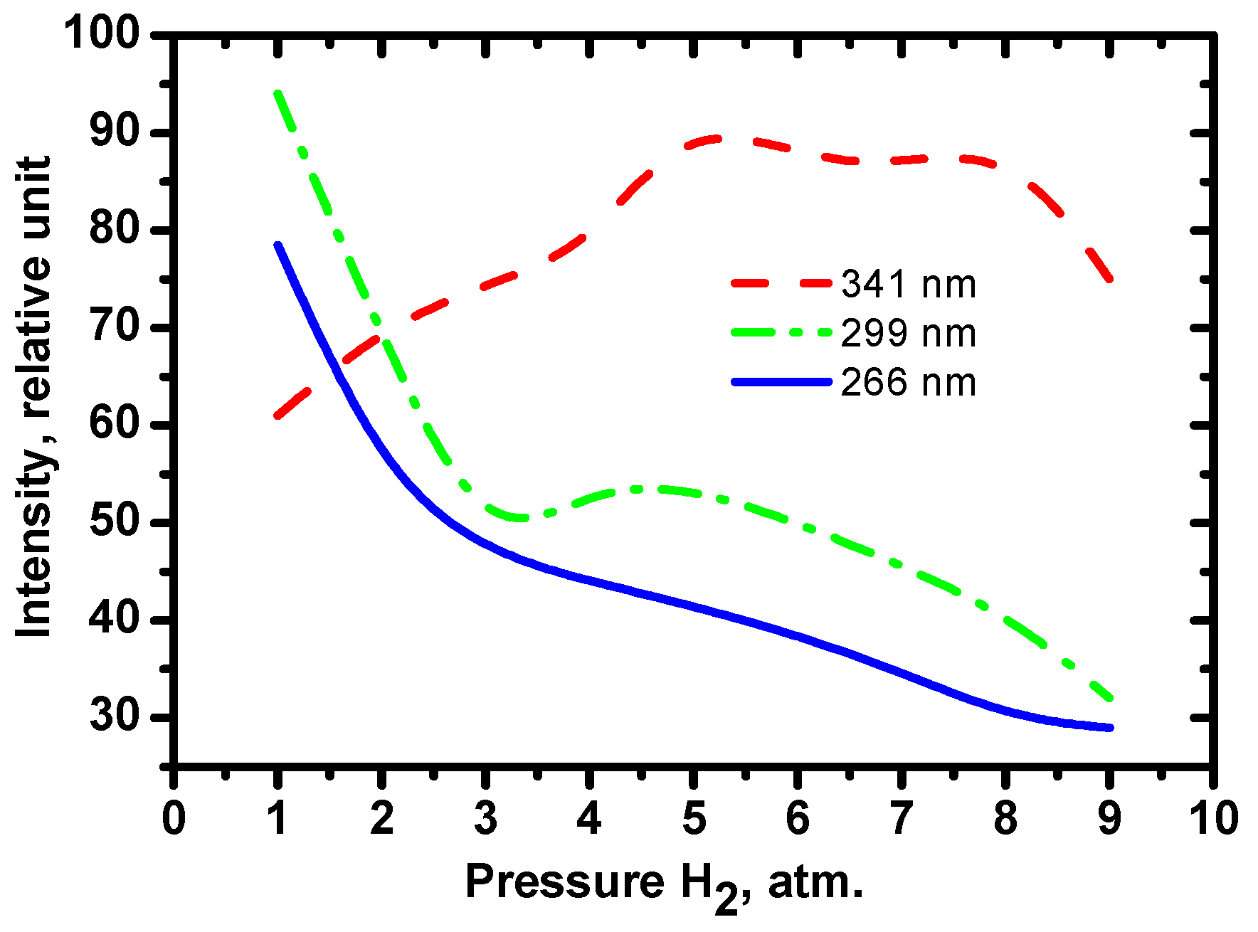
2.1. Selection of Wavelengths
2.2. Theoretical Base of the VDO Retrieval
+ (9.0281Е−20)·(Т(Н) − 273)2 − (3.5194Е−22)·(Т(Н) − 273)3
+ (6.8356Е−25)·(Т(Н) − 273)4 − (5.2918Е−8)·(Т(Н) − 273)5,
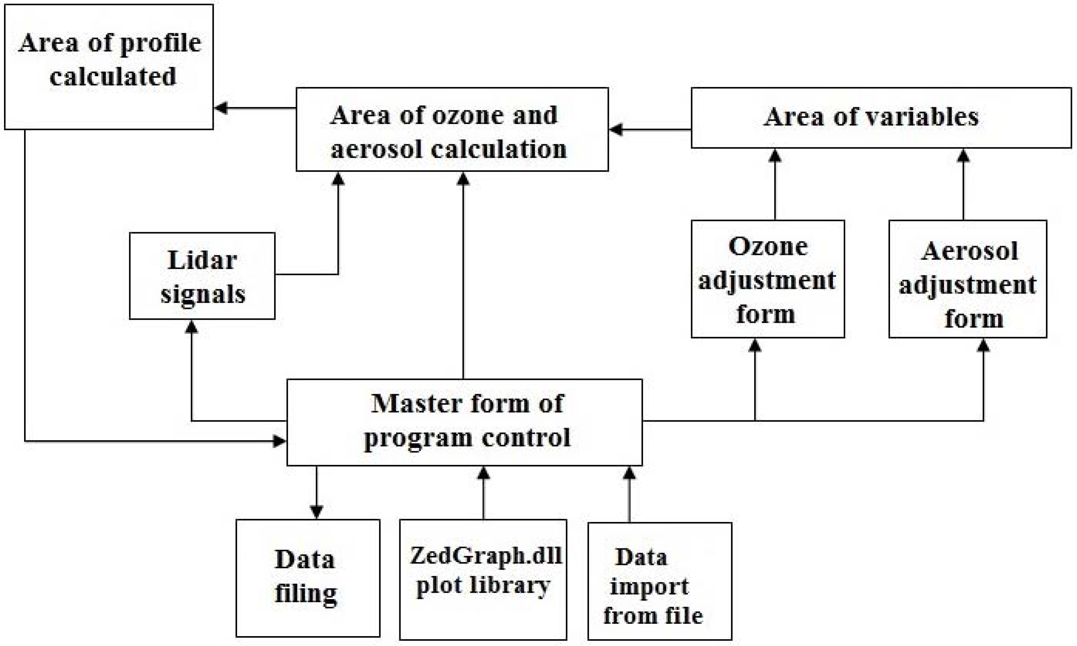
2.3. Software for VDO Retrieval
- Reading the lidar data;
- Recording the retrieval results in ASCII format;
- Moving average smoothing of lidar signals;
- Temperature and aerosol correction;
- Smoothing of the VDO retrieval results.
3. Materials
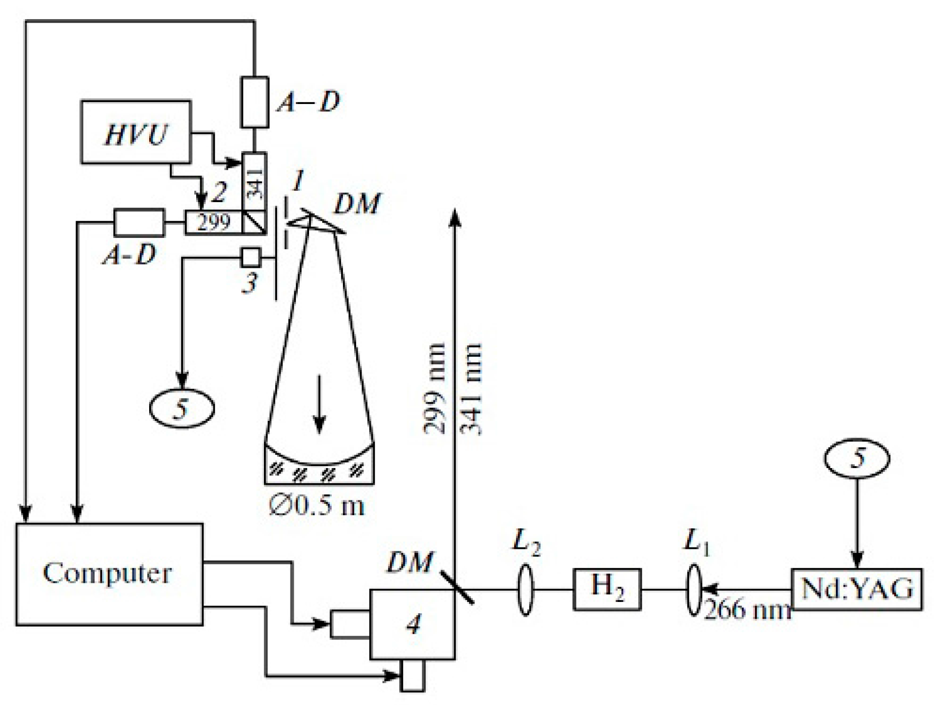
3.1. SLS Ozone Lidar
| 1 | Transmitter | |
| 2 | Sounding wavelength, λ, nm | 299, 341 |
| 3 | Pulse energy, mJ (corr. λ) | 25, 20 |
| 4 | Frequency, Hz (corr. λ) | 15 |
| 5 | Divergence, mrad | 0.1–0.3 |
| 6 | Receiver | |
| 7 | Mirror diameter, m | 0.5 |
| 8 | Focal length, m | 1.5 |
3.2. IASI/MetOp
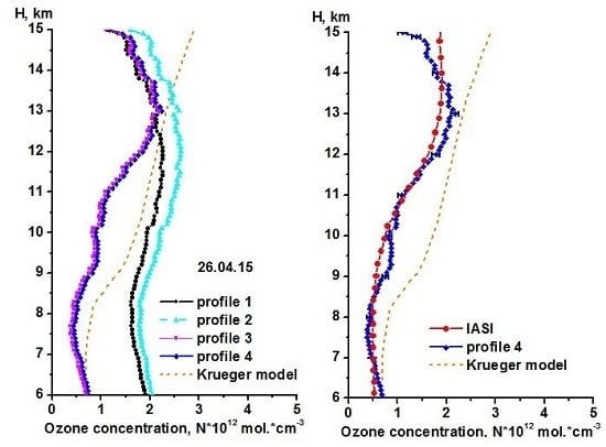
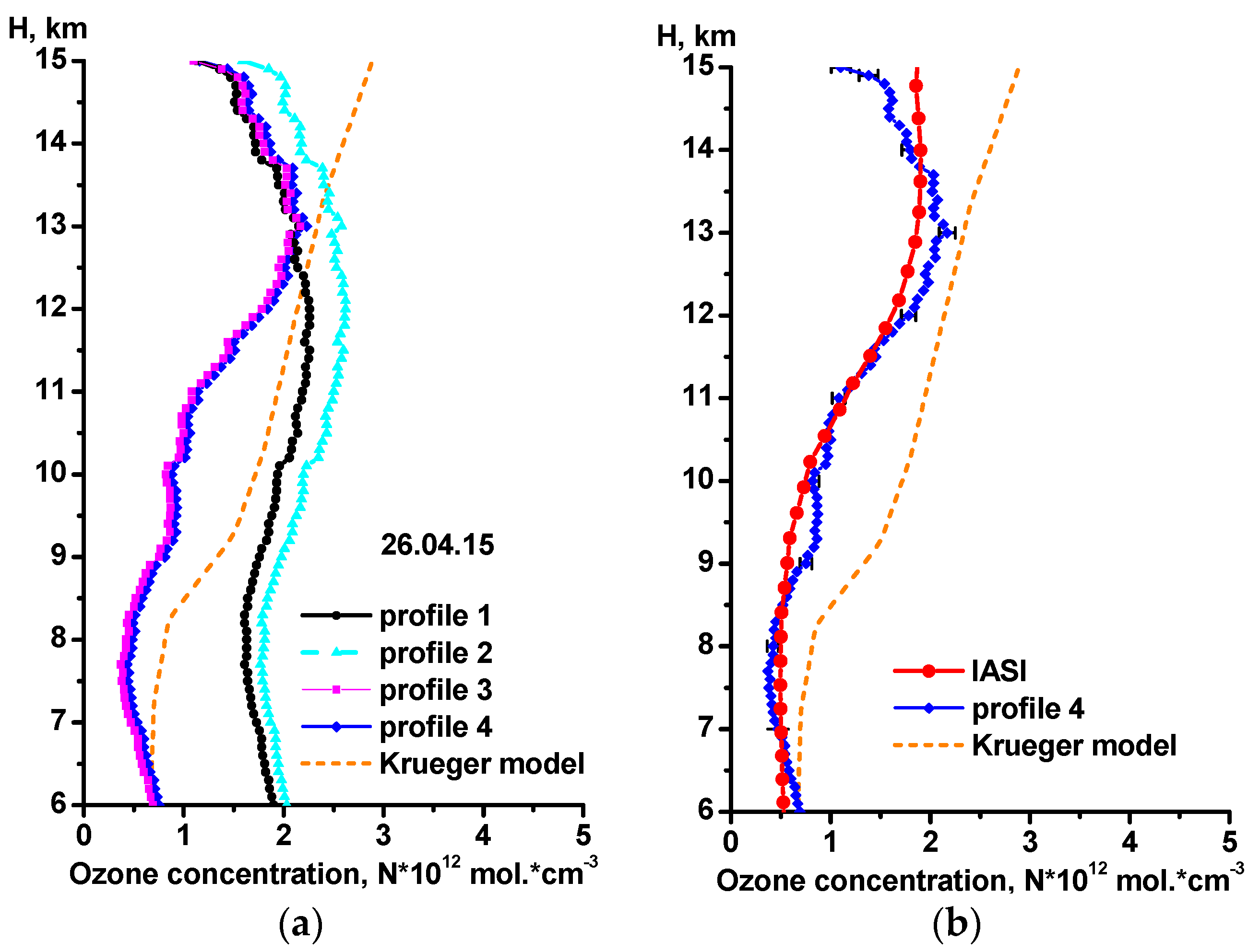
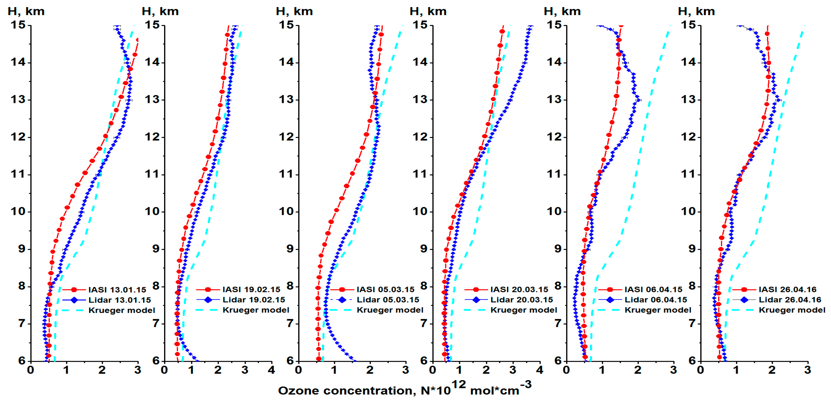
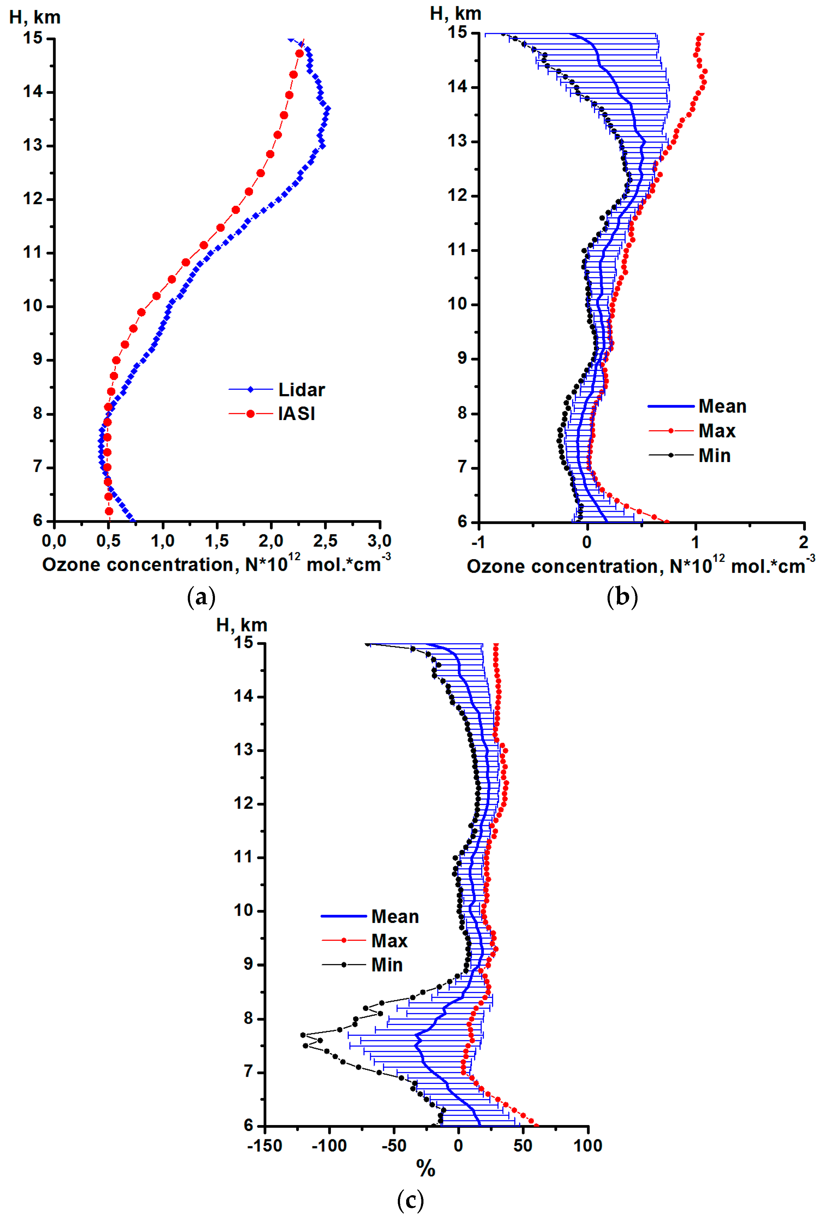
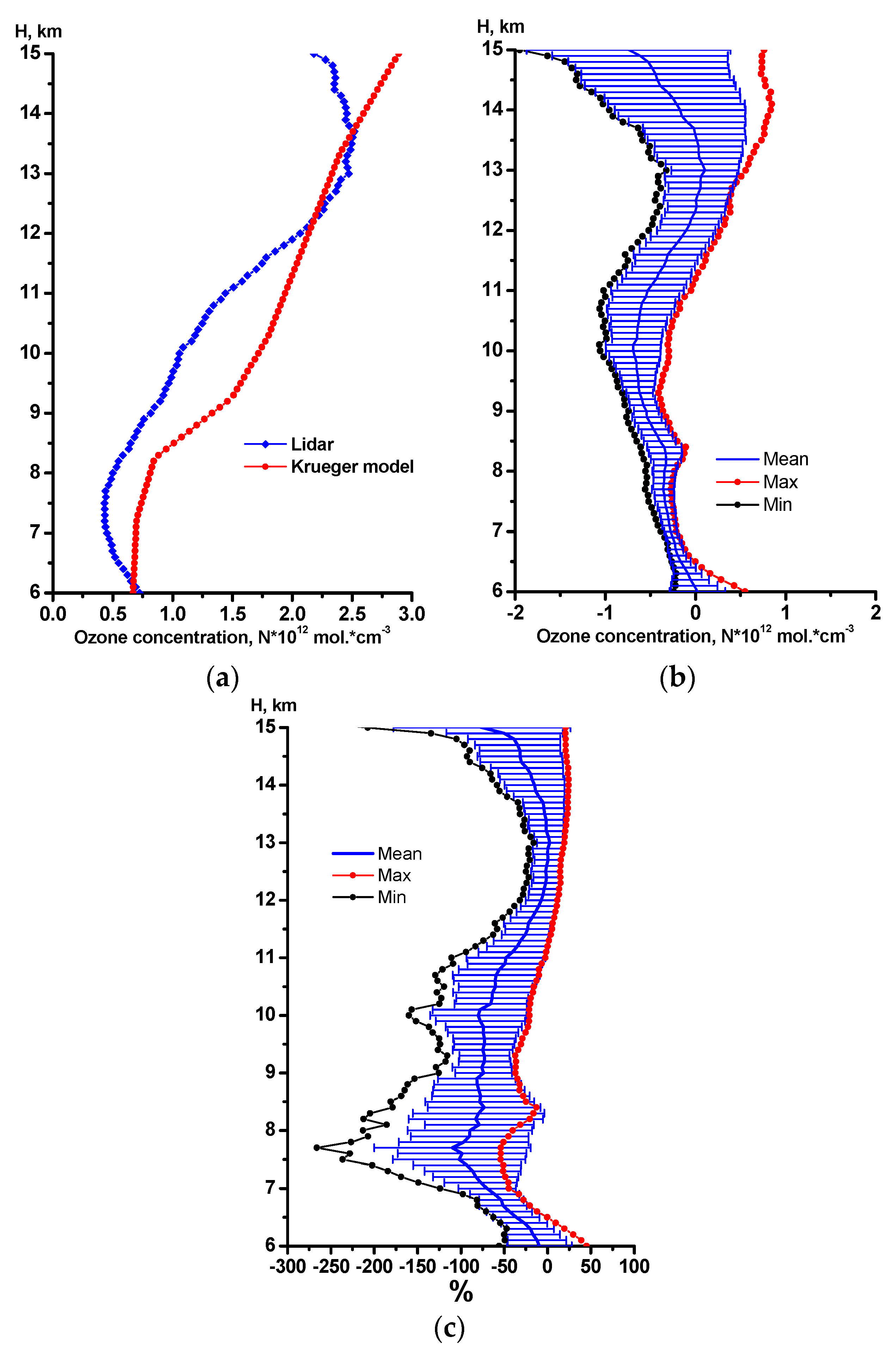
4. Results
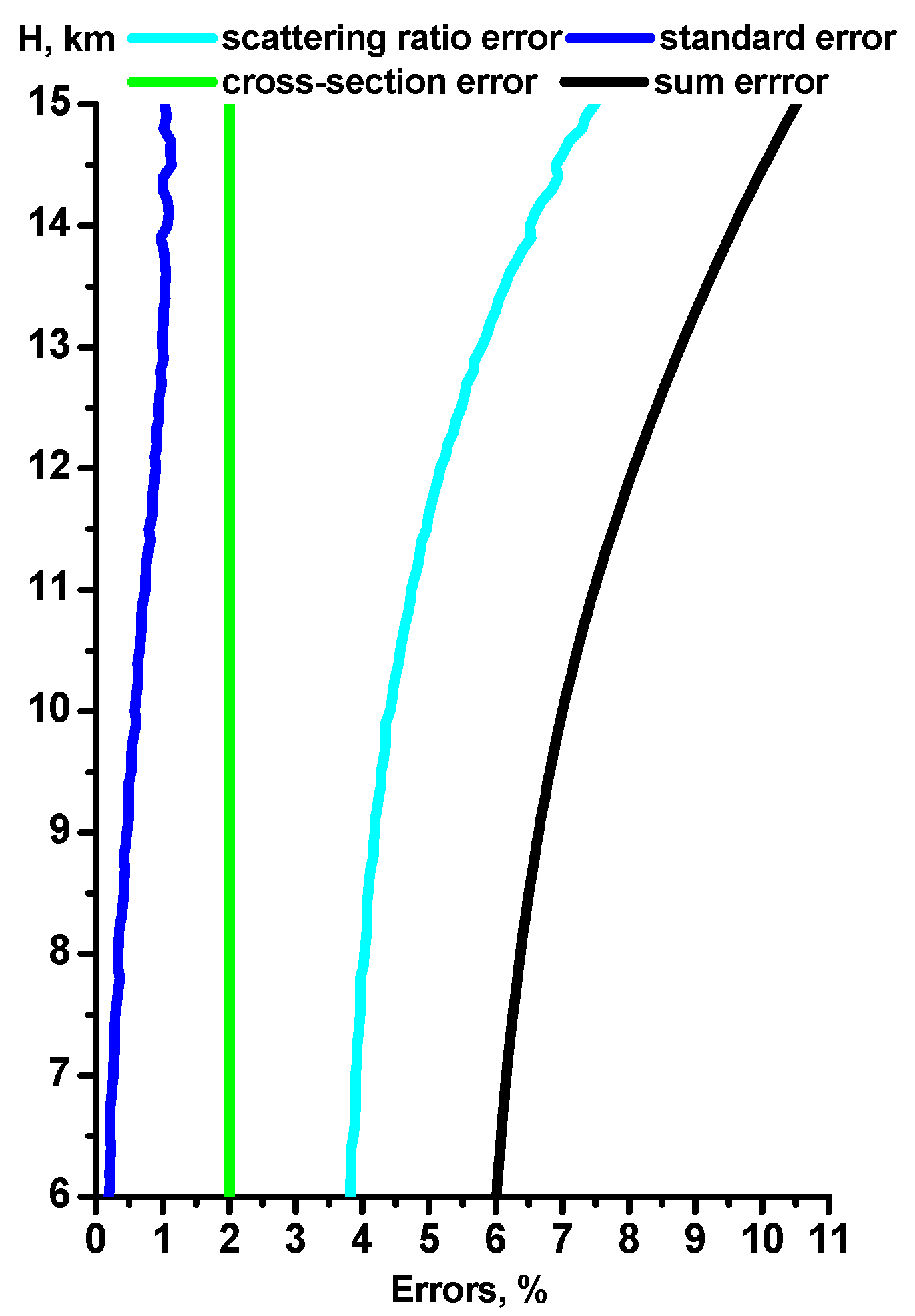
5. Discussion
6. Conclusions
Acknowledgments
Author Contributions
Conflicts of Interest
References
- Sullivan, J.T.; McGee, T.J.; Sumnicht, G.K.; Twigg, L.W.; Hoff, R.M. A mobile differential absorption lidar to measure sub-hourly fluctuation of tropospheric ozone profiles in the Baltimore–Washington, D.C. Atmos. Meas. Tech. 2014, 7, 3529–3548. [Google Scholar] [CrossRef]
- Repasky, K.S.; Moen, D.; Spuler, S.; Nehrir, A.R.; Carlsten, J.L. Progress towards an autonomous field deployable diode-laser-based differential absorption lidar (DIAL) for profiling water vapor in the lower troposphere. Remote Sens. 2013, 6, 6241–6259. [Google Scholar] [CrossRef]
- Queißer, M.; Burton, M.; Fiorani, L. Differential absorption lidar for volcanic CO2 sensing tested in an unstable atmosphere. Opt. Exp. 2015, 23. [Google Scholar] [CrossRef] [PubMed]
- Galani, E.; Balis, D.; Zanis, P.; Zerefos, C.; Papayannis, A.; Wernli, H.; Gerasopoulo, E. Observations of stratosphere-to-troposphere transport events over the eastern Mediterranean using a ground-based lidar system. J. Geophys. Res. 2013, 108, 6634–6644. [Google Scholar] [CrossRef]
- Nakazato, M.; Nagai, T.; Sakai, T.; Hirose, Y. Tropospheric ozone differential-absorption lidar using stimulated Raman scattering in carbon dioxide. Appl. Opt. 2007, 46, 2269–2279. [Google Scholar] [CrossRef] [PubMed]
- Bukreev, V.S.; Vartapetov, S.K.; Veselovskii, I.A.; Galustov, A.S.; Kovalev, Y.M.; Prokhorov, A.M.; Svetogorov, E.S.; Khemelevtsov, S.S. Excimer-laser-based lidar system for stratospheric and tropospheric ozone measurements. Quantum Electron. 1994, 21, 591–596. [Google Scholar]
- Eisele, H.; Scheel, H.E.; Sladkovic, R.; Trickl, T. High resolution lidar measurements of stratosphere-troposphere exchange. J. Atmos. Sci. 1999, 56, 319–330. [Google Scholar] [CrossRef]
- Pommier, M.; Clerbaux, C.; Law, K.S.; Ancellet, G.; Bernath, P.; Coheur, P.F.; Hadji-Lazaro, J.; Hurtmans, D.; Nedelec, P.; Paris, J.D.; et al. Analysis of IASI tropospheric O3 data over Arctic during POLARCAT campaigns in 2008. Atmos. Chem. Phys. 2012, 12, 7371–7389. [Google Scholar] [CrossRef]
- Gazeaux, J.; Clerbaux, C.; George, M.; Hadji-Lazaro, J.; Kuttippurath, J.; Coheur, P.F.; Hurtmans, D.; Deshler, T.; Kovilakam, M.; Campbell, P.; et al. Intercomparison of polar ozone profiles by IASI/MetOp sounder with 2010 Concordiasiozonesonde observations. Atmos. Meas. Tech. 2013, 6, 613–620. [Google Scholar] [CrossRef]
- Viatte, C.; Schneider, M.; Redondas, A.; Hase, F.; Eremenko, M.; Chelin, P; Flaud, J.M.; Blumenstock, T.; Orphal, J. Comparison of ground-based FTIR and Brewer O3 total column with data from two different IASI algorithms and from OMI and GOME-2 satellite instruments. Atmos. Meas. Tech. 2011, 4, 535–546. [Google Scholar] [CrossRef]
- Molina, L.T.; Molina, M.T. Absolute absorption cross section of ozone in the 185 nm to 350 nm wavelengthrange. J. Geophys. Res. 1988, 91, 14501–14508. [Google Scholar] [CrossRef]
- El’nikov, A.V.; Zuev, V.V.; Marichev, V.N.; Tsaregorodtsev, S.I. First results of lidar observations of stratospheric ozone above western Siberia. Atmos. Ocean.Opt. 1989, 2, 841–842. [Google Scholar]
- McDermid, I.S.; Walsh, T.D.; Deslis, A.; White, M.L. Optical systems design for a stratospheric lidar system. Appl. Opt. 1995, 34, 6201–6210. [Google Scholar] [CrossRef] [PubMed]
- Godin, S.; David, C.; Lakoste, A.M. Systematic ozone and aerosol lidar measurements at OHP (44°N, 6°E) and Dumont. In Proceedings of the Abstracts of Papers: 17th International Laser Radar Conference, Sendai, Japan, 25–29 July 1994; pp. 409–412. [Google Scholar]
- Claude, H.; Scönenborn, F.; Streinbrecht, W.; Vandersee, W. DIAL ozone measurements at the Met. Obs. Hohenpeiβenberg: Climatology and trends. In Proceedings of the Abstracts of Papers: 17th International Laser Radar Conference, Sendai, Japan, 25–29 July 1994; pp. 413–415. [Google Scholar]
- Stefanutti, L.; Castagnoli, F.; Guasta, D.M.; Morandi, M.; Sacco, V.M.; Zuccagnoli, L.; Godin, S.; Megie, G.; Porteneuve, J. A four-wavelength depolarization backscattering LIDAR for IISC monitoring. Appl. Phys. B 1992, 55, 13–17. [Google Scholar] [CrossRef]
- Pazmino, A.F.; Lavorato, M.B.; Fochesatto, G.J. DIAL system for measurements of stratospheric ozone at Buenos Aires. In Advances in Laser Remote Sensing, Proceedings of the Selected Papers Presented at the 20th ILRC, Vichy, France, 10–14 July 2000; Ecole Polytechnique Impr: Paris, France, 2001. [Google Scholar]
- Malicet, J.; Daumont, D.; Charbonnier, J.; Parisse, C.; Chakir, A.; Brion, J. Ozone UV spectroscopy. II. Absorption cross-sections and temperature dependence. J. Atmos. Chem. 1995, 21, 263–273. [Google Scholar] [CrossRef]
- Zhu, H.; Qu, Z.W.; Grebenshchikov, S.Y.; Schinke, R.; Malicet, J.; Brion, J.; Daumont, D. Huggins band of ozone: Assignment of hot bands. J. Chem. Phys. 2005, 122. [Google Scholar] [CrossRef] [PubMed]
- Clerbaux, C.; Boynard, A.; Clarisse, L.; George, M.; Hadji-Lazaro, J.; Herbin, H.; Hurtmans, D.; Pommier, M.; Razavi, A.; Turquety, S.; et al. Monitoring of atmospheric composition using the thermal infrared IASI/MetOp sounder. Atmos. Chem. Phys. 2009, 9, 6041–6054. [Google Scholar] [CrossRef]
- Matvienko, G.G.; Belan, B.D.; Panchenko, M.V.; Romanovskii, O.A.; Sakerin, S.M.; Kabanov, D.M.; Turchinovich, S.A.; Turchinovich, Y.S.; Eremina, T.A.; Kozlov, V.S.; et al. Complex experiment on studying the microphysical, chemical, and optical properties of aerosol particles and estimating the contribution of atmospheric aerosol-to-earth radiation budget. Atmos. Meas. Tech. 2015, 8, 4507–4520. [Google Scholar] [CrossRef]
- August, T.; Klaes, D.; Schlüssel, P.; Hultberg, T.; Crapeau, M.; Arriaga, A.; O’Carroll, A.; Coppens, D.; Munro, R.; Calbet, X. IASI on Metop-A: Operational Level 2 retrievals after five years in orbit. J. Quant. Spectrosc. Radiat. Trans. 2012, 113, 1340–1371. [Google Scholar] [CrossRef]
- Keim, C.; Eremenko, M.; Orphal, J.; Dufour, G.; Flaud, J.M.; Höpfner, M.; Boynard, A.; Clerbaux, C.; Payan, S.; Coheur, P.F.; et al. Tropospheric ozone from IASI: Comparison of different inversion algorithms and validation with ozone sondes in the northern middle latitudes. Atmos. Chem. Phys. 2009, 9, 9329–9347. [Google Scholar] [CrossRef]
- Krueger, A.J.; Minzner, R.A. Mid-latitude ozone model for the 1976 U.S. Standard Atmosphere. J. Geophys. Res. 1976, 81, 4477–4488. [Google Scholar] [CrossRef]


| Country, Observations Site | Start of Measu-Rements | Radiation Source: Wavelength, nm/Pulse Energy, mJ/Pulse Repetition Frequency, Hz | Receiving Mirror (Diameter), m | Ref. |
|---|---|---|---|---|
| Russia, Tomsk (56.5°N, 85°E) | 1989 | XeCl + SRS (H2) 308/100/100; 353/50/1000 | 2.2 0.5 0.3 | [12] |
| USA, California (34°N, 118°E) | 1986 | XeCl + SRS (H2) 308–353 | 0.9 | [13] |
| France, Provanсe (44°N, 6°E) | 1986 | XeCl+ Nd:YAG 308/250/50; 355/150/50 | 4 mirrors of 0.53 | [14] |
| Germany, Hohenpeiβenberg (48°N, 11°E) | 1987 | XeCl + SRS (H2) 308/300/20; 353/150/20 | 0.9 | [15] |
| France, Italia, the Antarctic (66°S, 140°E) | 1991 | XeCl+ Nd:YAG 308/180/80; 355/150/10 | 0.8 | [16] |
| Argentina, Buenos-Aires (35°S, 59°W) | 1999 | XeCl+ Nd:YAG 308/300/100; 355/255/10 | 0.5 | [17] |
| Pumping Radiation | Wavelength, nm | ||
|---|---|---|---|
| H2 C1 C2 | D2 C1 C2 C3 | CO2 C1 C2 | |
| Nd:YAG, 266 nm | 299 341 | 289 316 | 287 299 |
| KrF, 248 nm | 277 313 | 268 291 319 | |
| Wavelength, nm | Temperature, K | ||||
|---|---|---|---|---|---|
| 218 | 228 | 243 | 273 | 295 | |
| On line | |||||
| 299 | 4.1 × 10⁻¹⁹ | 4.1 × 10⁻¹⁹ | 4.25 × 10⁻¹⁹ | 4.3 × 10⁻¹⁹ | 4.6 × 10⁻¹⁹ |
| Off line | |||||
| 341 | 6 × 10⁻²² | 6 × 10⁻²² | 6 × 10⁻²² | 6 × 10⁻²² | 1.2 × 10⁻²¹ |
| Date | Siberian Lidar Station | MetOp (IASI) Satellite | ||
|---|---|---|---|---|
| Greenwich Time | Coordinates (56.5°N, 85.0°E) | Greenwich Time | Coordinates | |
| 13 January 2015 | 11:53–13:45 | 14:17 | 56.472°N, 85.387°E | |
| 19 February 2015 | 12:39–14:13 | 14:53 | 56.681°N, 85.164°E | |
| 5 March 2015 | 13:05–14:56 | 15:02 | 56.472°N, 85.118°E | |
| 20 March 2015 | 13:32–15:24 | 14:53 | 56.691°N, 85.124°E | |
| 6 April 2015 | 14:25–16:17 | 15:41 | 56.254°N, 84.935°E | |
| 26 April 2015 | 15:11–17:03 | 15:26 | 56.585°N, 84.594°E | |
© 2017 by the authors. Licensee MDPI, Basel, Switzerland. This article is an open access article distributed under the terms and conditions of the Creative Commons Attribution (CC BY) license (http://creativecommons.org/licenses/by/4.0/).
Share and Cite
Dolgii, S.I.; Nevzorov, A.A.; Nevzorov, A.V.; Romanovskii, O.A.; Kharchenko, O.V. Intercomparison of Ozone Vertical Profile Measurements by Differential Absorption Lidar and IASI/MetOp Satellite in the Upper Troposphere–Lower Stratosphere. Remote Sens. 2017, 9, 447. https://doi.org/10.3390/rs9050447
Dolgii SI, Nevzorov AA, Nevzorov AV, Romanovskii OA, Kharchenko OV. Intercomparison of Ozone Vertical Profile Measurements by Differential Absorption Lidar and IASI/MetOp Satellite in the Upper Troposphere–Lower Stratosphere. Remote Sensing. 2017; 9(5):447. https://doi.org/10.3390/rs9050447
Chicago/Turabian StyleDolgii, Sergey I., Alexey A. Nevzorov, Alexey V. Nevzorov, Oleg A. Romanovskii, and Olga V. Kharchenko. 2017. "Intercomparison of Ozone Vertical Profile Measurements by Differential Absorption Lidar and IASI/MetOp Satellite in the Upper Troposphere–Lower Stratosphere" Remote Sensing 9, no. 5: 447. https://doi.org/10.3390/rs9050447