
Generic Methodology for Field Calibration of Nacelle-Based Wind Lidars


Abstract
:
1. Introduction
1.1. Profiling Lidars for Power Performance
1.2. The Need for Calibration Procedures
operation that, under specified conditions, in a first step, establishes a relation between the quantity values with measurement uncertainties provided by measurement standards and corresponding indications with associated measurement uncertainties and, in a second step, uses this information to establish a relation for obtaining a measurement result from an indication.
- Can (nacelle-based) wind lidars be calibrated via a generic procedure, independent of the lidar type or design?
- How to assess lidar measurement uncertainties?
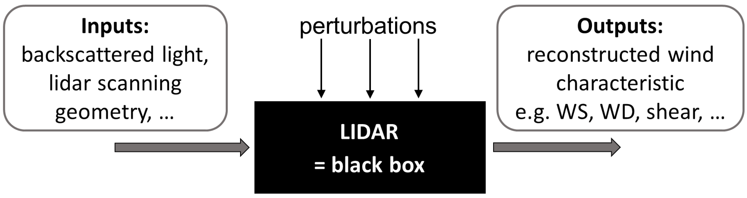
2. Two Plausible Calibration Concepts: The White- or the Black-Box
2.1. Black Box
- for horizontal wind speed and wind direction:
- −
- lidar placed on a platform high enough to allow the beam(s) to not be blocked by the ground in order for the reconstruction algorithm to be available. High stiffness of the tower is required to avoid significant deflections causing the lidar beams to constantly move and sense winds in locations unacceptably far from the reference instruments. This is the reason why we do not recommend calibrating lidars mounted on the nacelle of on an operating wind turbine. The beam perturbations would depend on both the turbine and the actual wind distribution during the testing period. Consequently the repeatability of the calibration would be seriously impaired and the uncertainties increased. For modern wind turbines, the rotor diameter is ∼100 m. Power performance standards (IEC 61400-12-1, [14]) require to measure the free wind at an upstream distance of . With a cone or half-opening angle of , the height of the platform should therefore be >2.5. In addition, a minimum height should be considered to account for the lidar probe volume and avoid sensing highly inhomogeneous and turbulent winds too close to the ground;
- −
- a mast with reference instruments (e.g., cup or sonic anemometers, wind vanes) mounted at the location where the lidar-reconstructed wind characteristics are estimated. For a two-beam lidar system, such a location may be at the point directly in between the two beam positions, or formally anywhere between the two beams (see Section 6.2);
- −
- accurate detection of the lidar beam or centreline, in order to position the reference instruments appropriately. This may be extremely difficult to achieve, particularly if no beam is physically present at the centre of the scanning pattern.
- for vertical wind shear and veer: reference wind speed and direction instruments located at several heights ranging between the minimum and maximum measurement heights of the lidar, e.g., from to .
2.2. White Box
- calibrate the LOS positioning: e.g., by calibrating the lidar’s internal inclinometers (if any), by verifying the geometry of the trajectory (opening angle between each LOS and the optical centreline), by verifying the measurement range;
- calibrate the lidar-measured ;
- propagate inputs’ uncertainties to the lidar-reconstructed wind characteristics.
2.3. Which Concept to Choose?
- multiple calibrated reference instruments (with certificates) are necessary to calibrate each of the reconstructed wind characteristics—e.g., cup anemometer for wind speed, vane for wind direction;
- the assumptions formulated in the reconstruction algorithms may not be completely justified and strongly related to the characteristics of the calibration site—e.g., flow homogeneity in complex terrain;
- the calibration procedure and setup is specific to the scanning trajectory of the lidar system and to each wind characteristic to calibrate (speed, direction, shear, etc.).
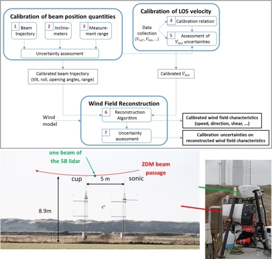
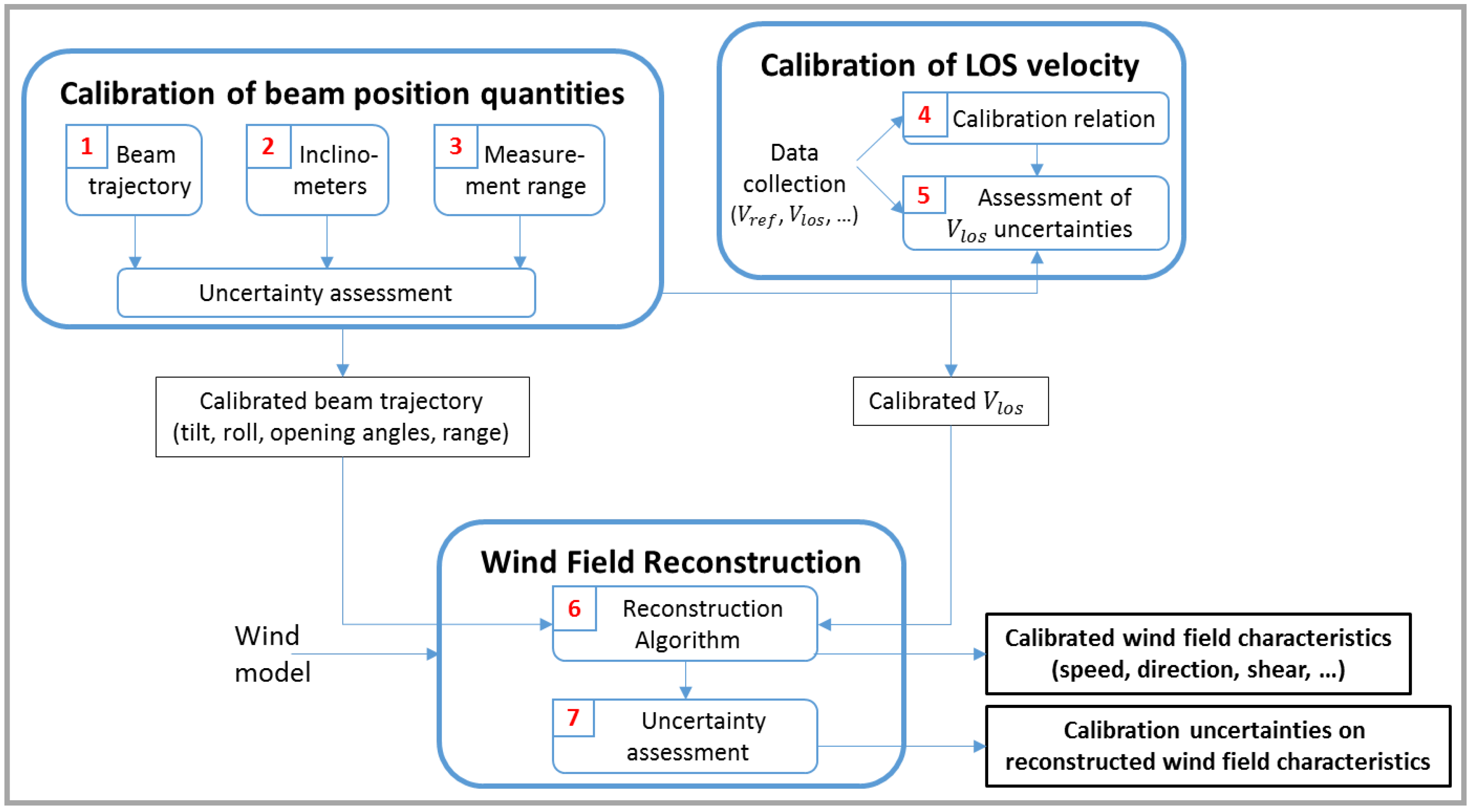
3. White Box Calibration: A Generic Methodology
4. Calibration/Verification of LOS Positioning Input Quantities
5. LOS Velocity Calibration and Uncertainties
5.1. Reference Quantity
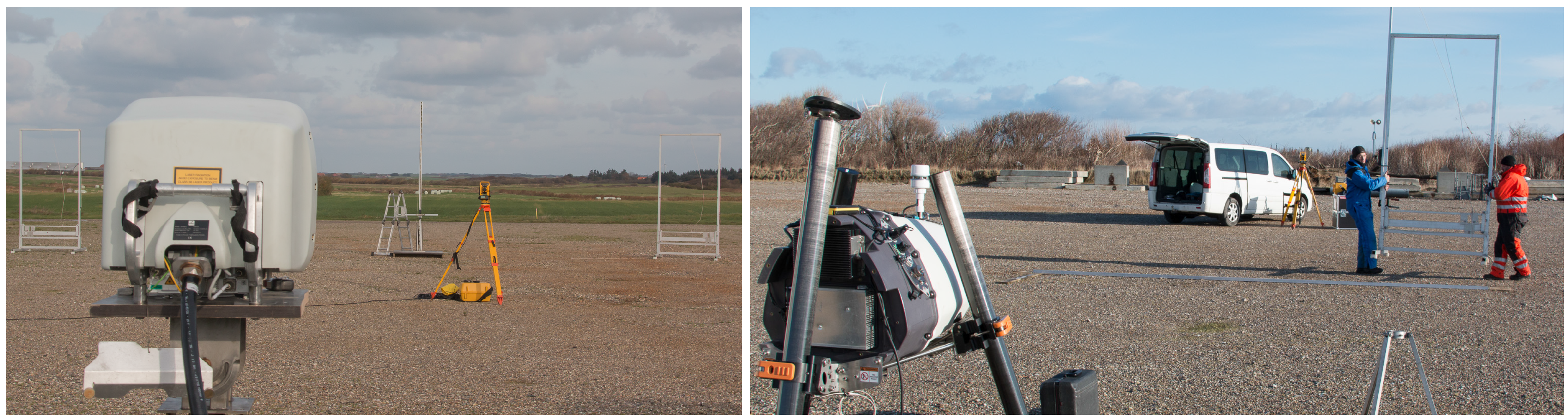
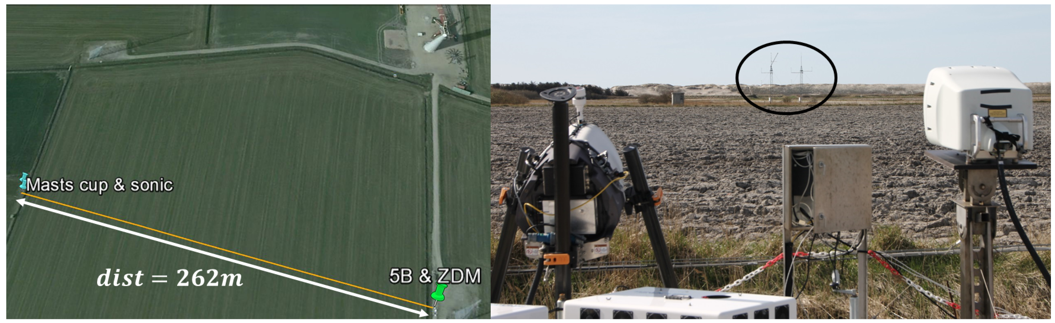
5.2. Measurement Setup
5.3. Data Filtering
- Mast:
- −
- Cup wind speed ms: corresponding to the range of wind speeds for which the cup anemometer is calibrated, in a wind tunnel;
- −
- Inflow angle (measured by sonic) : to limit the contamination of by the vertical wind speed;
- −
- wind direction θ measured by sonic anemometer : except for the 1st step of the LOS direction evaluation process (see Section 5.4), the direction sector is restricted due to the asymmetric geometry of the employed sonic anemometer that can cause flow distortion. Additionally, this corresponds well to normal operational conditions of nacelle lidars since the wind direction relative to the turbine’s yaw position is usually ;
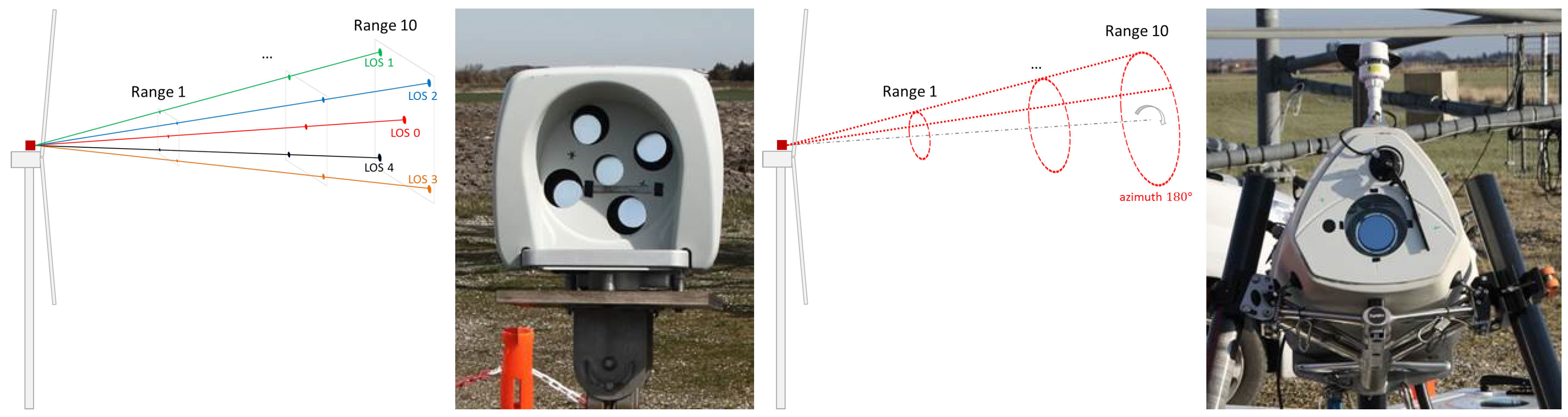
- 5B lidar: carrier-to-noise ratio > dB and LOS availability >95%. LOS availability is the ratio between successful and total attempts to measure . These two filters ensure the quality and quantity of data measured by the lidar for each 10-min period;
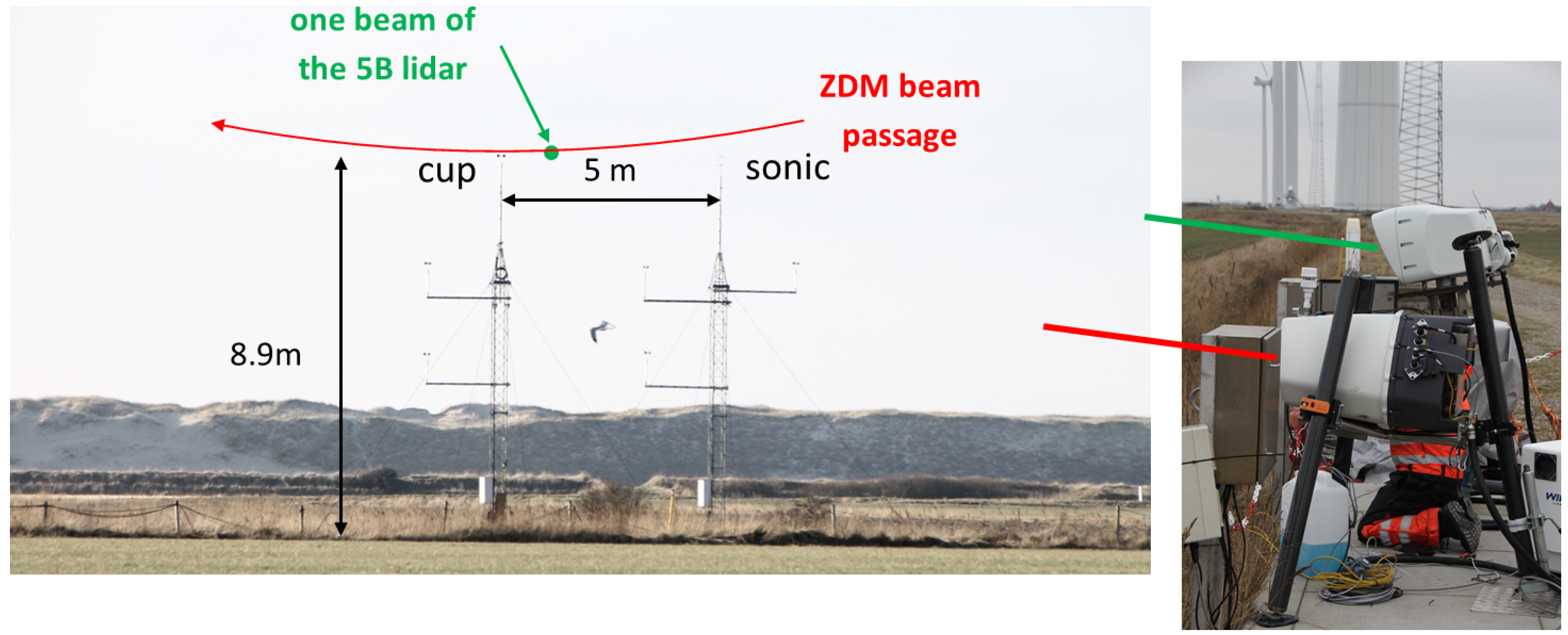
- ZDM lidar: LOS availability ≳75%. The LOS availability is obtained simultaneously to the averaging of high resolution (∼50 Hz) measurements contained in a specified azimuth sector, that we chose to be (i.e., the bottom of the ZDM scanning trajectory). Details on the employed averaging process can be found in [5]. Note that the lidar was stable enough to ensure the beam was not hitting the cup anemometer.
5.4. LOS Direction Evaluation
5.4.1. Fitting the Lidar Response to Wind Direction
- a cosine wave for a heterodyne lidar (such as 5B): ;
- a rectified cosine wave for a homodyne lidar (such as ZDM): . Homodyne lidars measure only the magnitude of the Doppler shift – not its sign – which translates into positive LOS velocities for any wind direction θ. In such a case, a rectified cosine must be used. The ambiguity in the fitting due to the two distinct solutions for is resolved by choosing the value corresponding to the expected bearing of the LOS, e.g., using GPS coordinates;
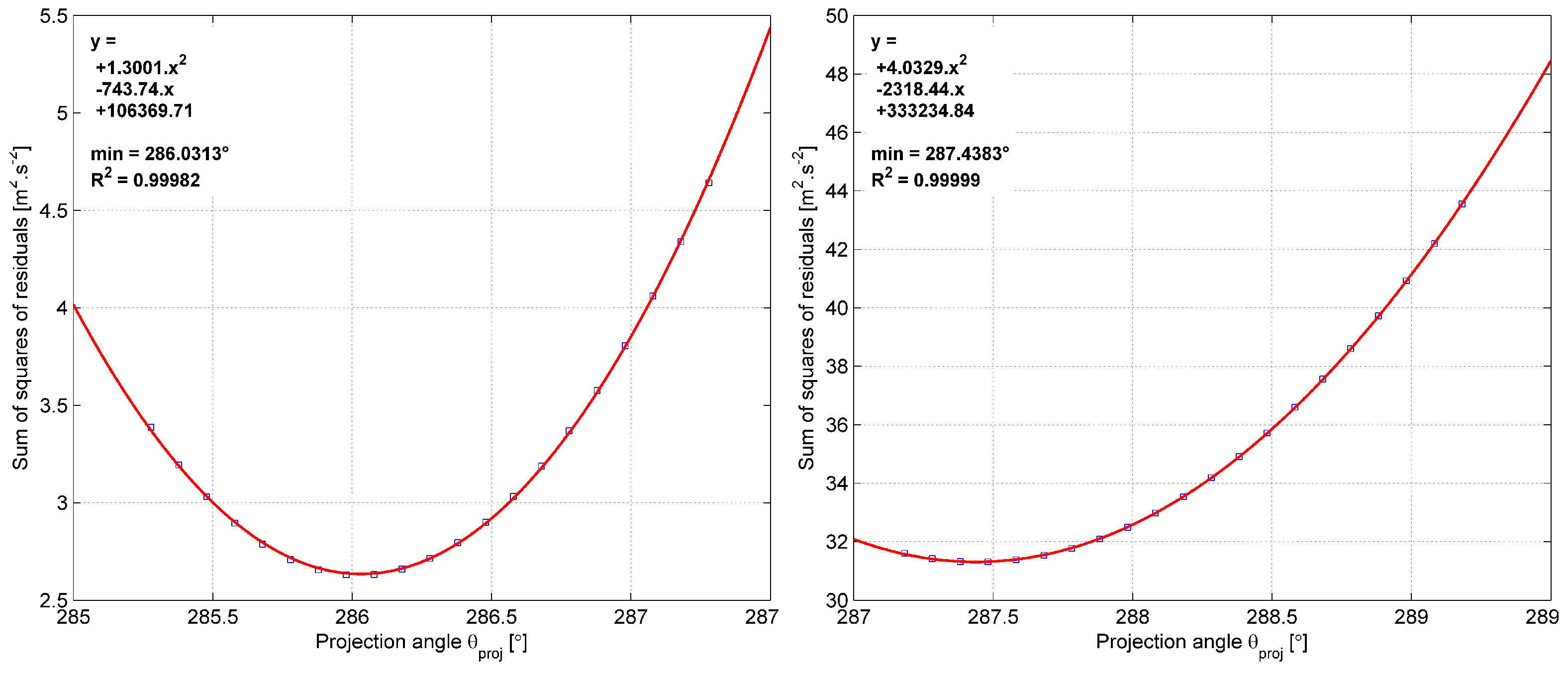
5.4.2. Refining the Estimated LOS Direction Using Residuals
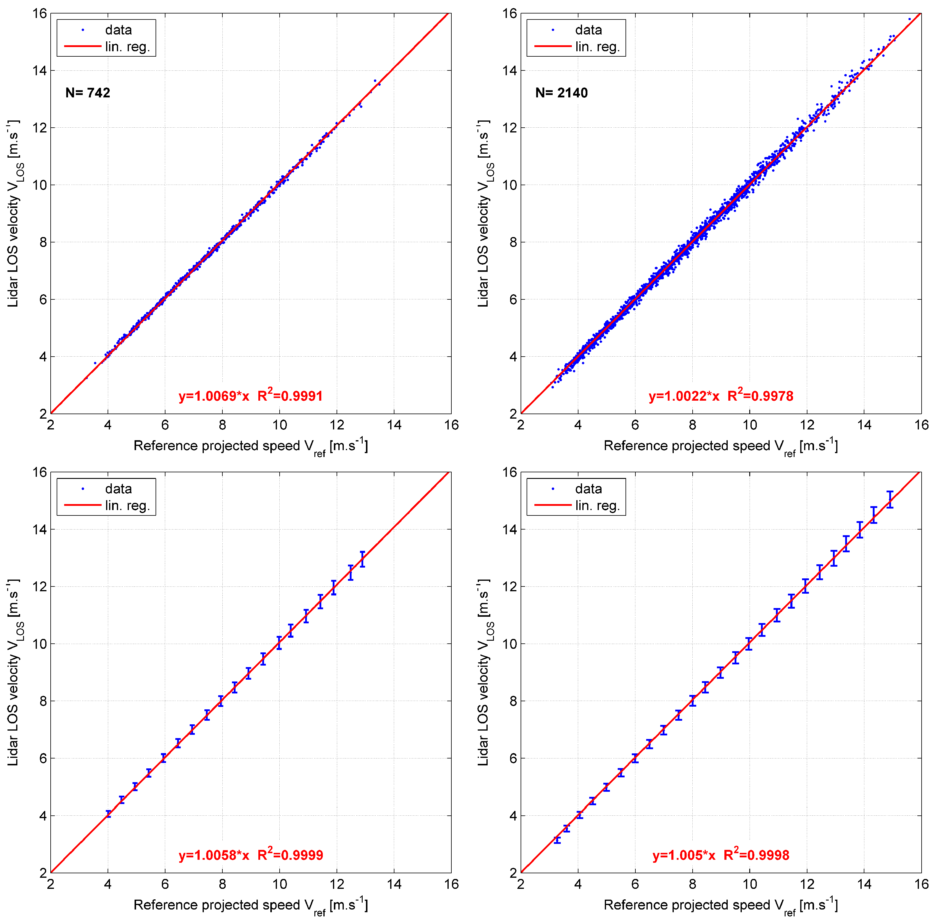
5.5. Calibration Relation
5.6. Measurement Uncertainties Assessment Procedure
5.6.1. Definition of uncertainty and the GUM methodology
non-negative parameter characterizing the dispersion of the quantity values being attributed to a measurand, based on the information used.
- define the measurement model: where y is the best estimate and are the input quantities;
- list the input quantities and determine their uncertainties ;
- evaluate covariances between the uncertainties of the input quantities;
- calculate the measured value y;
- combine the uncertainties on the input quantities using the law of propagation of uncertainties to obtain ;
- derive and report the expanded uncertainty where k is the coverage factor (see definition 2.38 in [11]).
5.6.2. Applying the GUM to the Calibration of
5.6.3. Combined Uncertainty on
5.6.4. Uncertainty Sources and Budget
- (i)
- Wind tunnel calibration uncertainty:where is the uncertainty specified by the calibration certificate for a coverage factor . We used 0.025 ms. The 2nd term is due to the variability of cup anemometers calibration results for Measnet accredited wind tunnels. Measnet requires the tunnels to be within % of each other. Hence a 1% uncertainty is added with an assumed rectangular—or uniform—distribution of uncertainty yielding the factor.
- (ii)
- Operational—also called classification—uncertainty:where is the anemometer’s classification number characterising the systematic deviations due to environmental conditions, e.g., angular response, turbulence, temperature (influence on bearing friction), etc. The cup anemometer used in this study is of type ‘Thies First Class Advanced’ which has a class of 0.9A ().
- (iii)
- Mounting uncertainty:related to the mounting of the sensor on the mast. The uncertainty is the default value for top-mounted instruments suggested in the revision of the IEC 61400-12-1.
- (i)
- LOS direction uncertainty, related to the statistical evaluation of (Section 5.4) and roughly estimated to:
- (ii)
- (iii)
- Vertical beam positioning uncertainty: characterises how close to the reference instruments height the beam is positioned. Here, modelling the vertical shear profile with the power law, using a shear exponent , a height uncertainty at , the wind speed uncertainty due to the height error is:
- (iv)
- Inclined beam and range uncertainty: practically, the inclined beam implies that the laser light travels, within the probe volume, through a range of heights. The lidar thus senses different wind speeds if there is a wind shear. Additionally, the range uncertainty along the LOS moves the probe volume’s center slightly away from the reference instruments’ height. A model of this uncertainty can be found in Annex A of [18]. Configuring this model with the 5B and ZDM lidars setup in Høvsøre and a conservative 5 m range uncertainty, we obtained respectively:
- (v)
- Spatial separation uncertainty: the spatial separation between the two reference sensors infers an uncertainty whose magnitude increases with the separation distance. In our case, the two masts are 5 m apart and the terrain is flat. The spatial separation effects can reasonably be neglected.
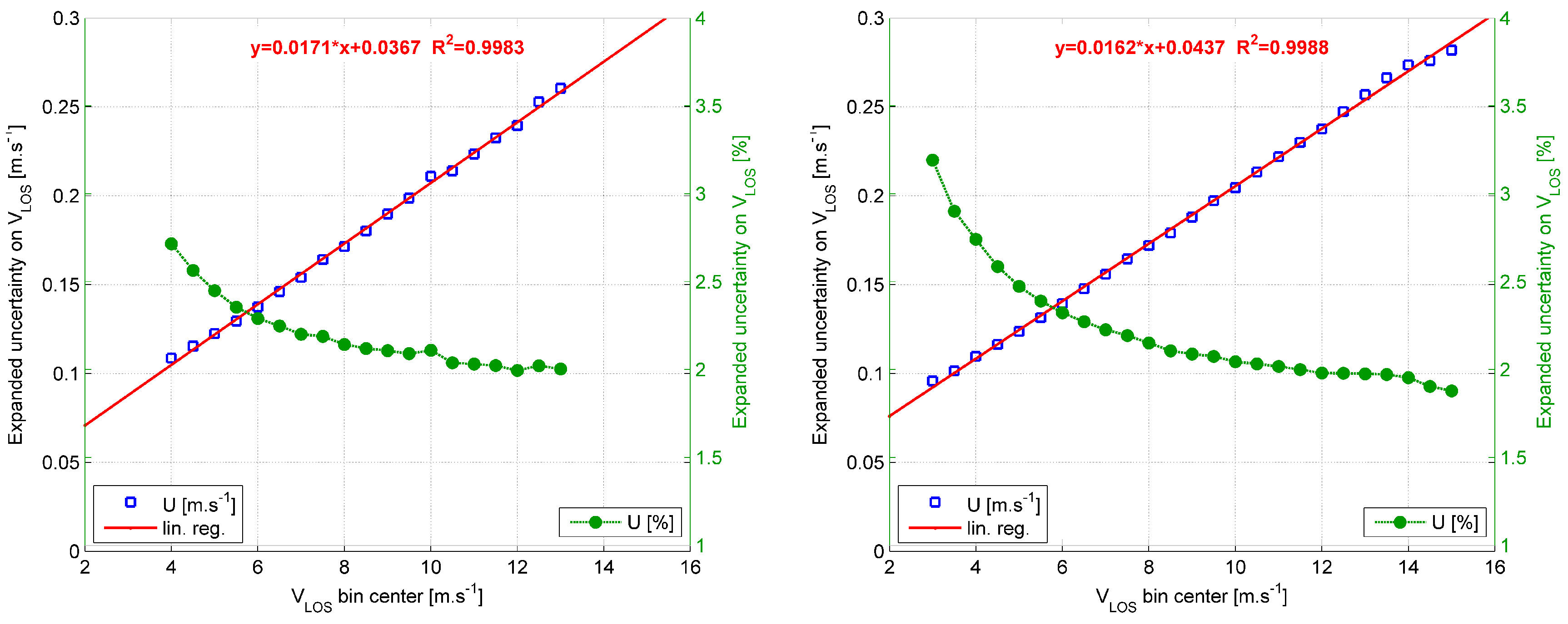
5.6.5. Expanded Uncertainties
5.7. Summary of Calibration Results
6. Uncertainties of Reconstructed Wind Characteristics
6.1. Wind Field Reconstruction Techniques
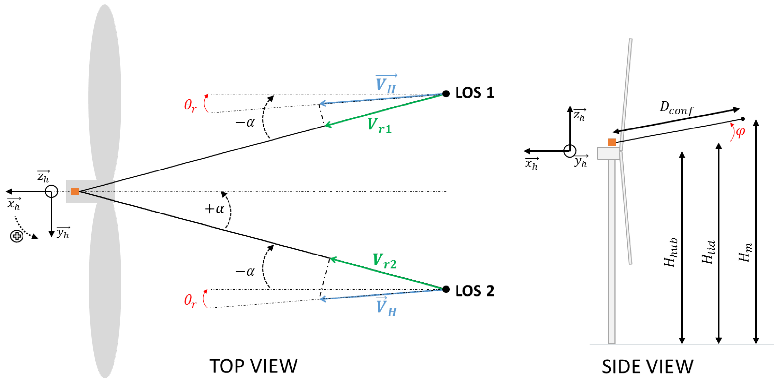
6.2. Example for a Two-Beam Nacelle Lidar
6.2.1. Reconstruction Algorithm
- (1)
- two-dimensional wind vector: the vertical component is 0, downstream and transverse components are denoted and respectively;
- (2)
- horizontal flow homogeneity: and are independent of the coordinates (see Figure 11) of the beams position;
- (3)
- the probe volume averaging is neglected: time-averaged lidar are considered as point-like quantities;
- (4)
- the lidar roll inclination is 0°: both beams sense winds at the same height.
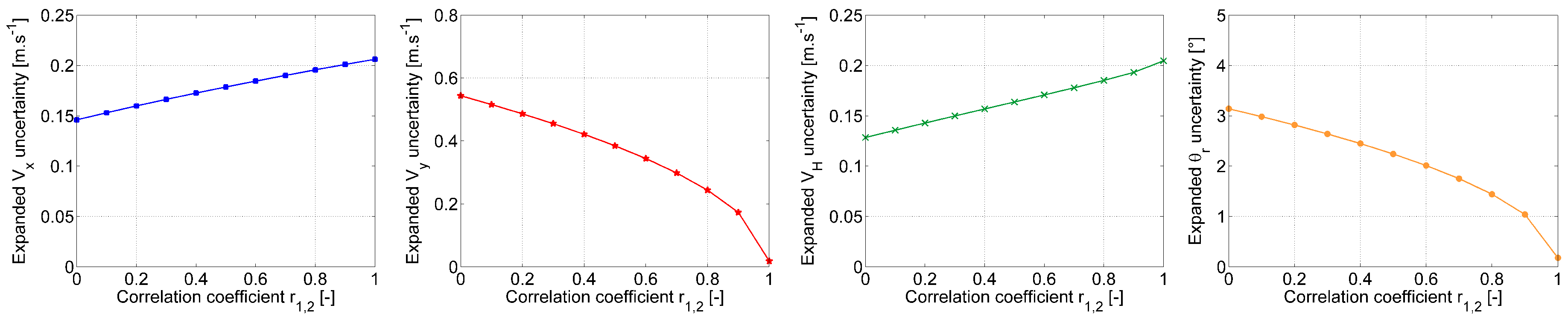
6.2.2. Propagating Uncertainties with the GUM
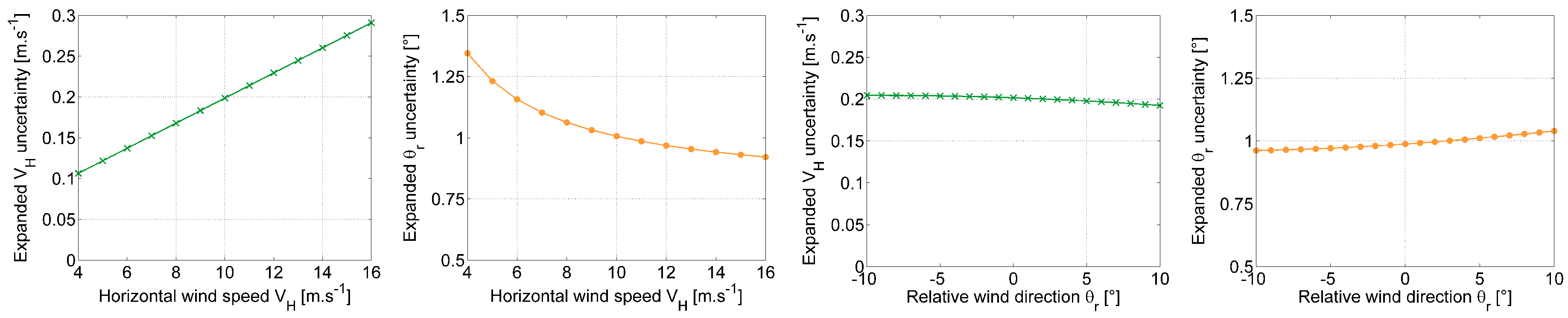
6.2.3. Uncertainty Budget, Results and Scale Analysis
- (i)
- LOS velocity: taking advantage of the previously observed linearity (see Section 5.6.5), the LOS velocity uncertainty of beam i is estimated to where and . We here obtained m and n by approximating the gain and offset value of the expanded uncertainty linear relation (see Table 1 ) and dividing it by the coverage factor;
- (ii)
- Tilt inclination: as prescribed by the inclinometers calibration;
- (iii)
- Opening angle: from the geometry verification, we estimate .
7. Discussion
7.1. On Lidar Uncertainties
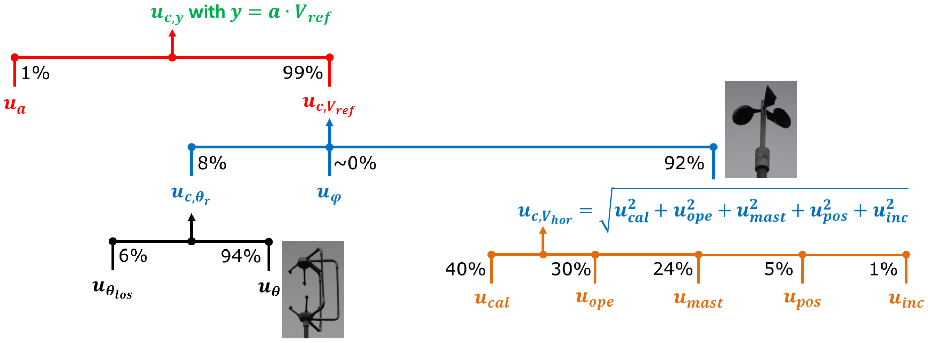
- (1)
- the uncertainty of the reference quantity accounts for of the combined LOS velocity uncertainty ;
- (2)
- >90% of the reference speed uncertainty is related to the combined reference HWS uncertainty ;
- (3)
- ∼94% of is due to the cup anemometer’s calibration, operational and mast uncertainties. The LOS velocity calibration process accounts only for the remaining with and .
7.2. On Repeatability in Field Measurements
7.3. On Limitations of the Application of the White Box
8. Conclusions
Acknowledgments
Author Contributions
Conflicts of Interest
References
- Wagner, R.; Courtney, M.; Gottschall, J.; Lindelöw, P. Accounting for the speed shear in wind turbine power performance measurement. Wind Energy 2011, 14, 993–1004. [Google Scholar] [CrossRef]
- Peña, A.; Hasager, C.B.; Gryning, S.E.; Courtney, M.; Antoniou, I.; Mikkelsen, T. Offshore wind profiling using light detection and ranging measurements. Wind Energy 2009, 12, 105–124. [Google Scholar] [CrossRef]
- Wagner, R.; Pedersen, T.; Courtney, M.; Antoniou, I.; Davoust, S.; Rivera, R. Power curve measurement with a nacelle mounted lidar. Wind Energy 2014, 17, 1441–1453. [Google Scholar] [CrossRef]
- Borraccino, A.; Courtney, M. Calibration Report for Avent 5-Beam Demonstrator Lidar; Technical Report; DTU Wind Energy: Roskilde, Denmark, 2016. [Google Scholar]
- Borraccino, A.; Courtney, M. Calibration Report for ZephIR Dual Mode Lidar (Unit 351); Technical Report; DTU Wind Energy: Roskilde, Denmark, 2016. [Google Scholar]
- Hardesty, R.M.; Weber, B.F. Lidar measurement of turbulence encountered by horizontal-axis wind turbines. J. Atmos. Ocean. Technol. 1987, 4, 191–203. [Google Scholar] [CrossRef]
- Lawrence, T.R.; Wilson, D.J.; Craven, C.E.; Jones, I.P.; Huffaker, R.M.; Thomson, J.A.L. A laser velocimeter for remote wind sensing. Rev. Sci. Instrum. 1972, 43, 512. [Google Scholar] [CrossRef]
- Schlipf, D.; Rettenmeier, A.; Haizmann, F.; Hofsäß, M.; Courtney, M.; Cheng, P.W. Model based wind vector field reconstruction from lidar data. In Proceedings of the 11th German Wind Energy Conference (DEWEK 2012), Bremen, Germany, 7–8 November 2012.
- Sathe, A.; Banta, R.; Pauscher, L.; Vogstad, K.; Schlipf, D.; Wylie, S. Estimating Turbulence Statistics and Parameters from Ground- and Nacelle-Based Lidar Measurements: IEA Wind Expert Report; Grant No.: 0602-02486B; DTU Wind Energy: Roskilde, Denmark, 2015. [Google Scholar]
- Vasiljevic, N. A Time-Space Synchronization of Coherent Doppler Scanning Lidars for 3D Measurements of Wind Fields. Ph.D. Thesis, DTU Wind Energy, Roskilde, Denmark, 2014. [Google Scholar]
- Joint Committee for Guides in Metrology. International Vocabulary of Metrology—Basic and General Concepts and Associated Terms (VIM); Technical Report, 200:2012; Bureau International des Poids et Mesures (BIPM): Sèvres, France, 2012. [Google Scholar]
- Joint Committee for Guides in Metrology. Evaluation of Measurement Data—Guide to the Expression of Uncertainty in Measurement; Technical Report, 100:2008; Bureau International des Poids et Mesures (BIPM): Sèvres, France, 2008. [Google Scholar]
- Gottschall, J.; Courtney, M.; Wagner, R.; Jørgensen, H.E.; Antoniou, I. Lidar profilers in the context of wind energy—A verification procedure for traceable measurements. Wind Energy 2012, 15, 147–159. [Google Scholar] [CrossRef]
- International Electrotechnical Commission (IEC). Power Performance Measurements of Electricity Producing Wind Turbines; IEC 61400-12-1 Ed. 2.0:CCDV; International Electrotechnical Commission: Geneva, Switzerland, 2015. [Google Scholar]
- Wagner, R.; Courtney, M.S.; Pedersen, T.F.; Davoust, S. Uncertainty of power curve measurement with a two-beam nacelle-mounted lidar. Wind Energy 2016, 19, 1269–1287. [Google Scholar] [CrossRef]
- Joint Committee for Guides in Metrology. Evaluation of Measurement Data—Propagation of Distributions Using Monde Carlo Method; Technical Report, 101:2008; Bureau International des Poids et Mesures (BIPM): Sèvres, France, 2008. [Google Scholar]
- Peña, A.; Floors, R.; Sathe, A.; Gryning, S.E.; Wagner, R.; Courtney, M.S.; Larsén, X.G.; Hahmann, A.N.; Hasager, C.B. Ten years of boundary-layer and wind-power meteorology at Høvsøre, Denmark. Bound. Layer Meteorol. 2016, 158, 1–26. [Google Scholar] [CrossRef] [Green Version]
- Borraccino, A.; Courtney, M.; Wagner, R. Generic Methodology for Calibrating Profiling Nacelle Lidars; Technical Report; DTU Wind Energy: Roskilde, Denmark, 2015. [Google Scholar]
- Raach, S.; Schlipf, D.; Haizmann, F.; Cheng, P.W. Three dimensional dynamic model based wind field reconstruction from lidar data. J. Phys. Conf. Ser. 2014, 524, 012005. [Google Scholar] [CrossRef]
- Towers, P.; Jones, B.L. Real-time wind field reconstruction from LiDAR measurements using a dynamic wind model and state estimation. Wind Energy 2016, 19, 133–150. [Google Scholar] [CrossRef]


| Lidar | LOS | Calibration Relation | Expanded Uncertainties () | |||||
|---|---|---|---|---|---|---|---|---|
| a | U (ms) | U at 4 ms | U at 16 ms | |||||
| 5B | LOS 0 | 286.03° | 1.0058 | 0.9999 | 742 | |||
| LOS 1 | 285.99° | 1.0072 | 0.9999 | 502 | ||||
| LOS 2 | 285.99° | 1.0084 | 1.0000 | 1087 | ||||
| LOS 3 | 286.06° | 1.0090 | 0.9999 | 446 | ||||
| LOS 4 | 285.99° | 1.0059 | 1.0000 | 1508 | ||||
| ZDM | 179°–181° | 287.44° | 1.0050 | 0.9998 | 2140 | 2.75% | ||
| azimuth | ||||||||
| Combined Uncertainty | Uncertainty Term and Order of Magnitude | ||||
|---|---|---|---|---|---|
| in | |||||
| in | |||||
| in | |||||
| in | |||||
© 2016 by the authors; licensee MDPI, Basel, Switzerland. This article is an open access article distributed under the terms and conditions of the Creative Commons Attribution (CC-BY) license (http://creativecommons.org/licenses/by/4.0/).
Share and Cite
Borraccino, A.; Courtney, M.; Wagner, R. Generic Methodology for Field Calibration of Nacelle-Based Wind Lidars. Remote Sens. 2016, 8, 907. https://doi.org/10.3390/rs8110907
Borraccino A, Courtney M, Wagner R. Generic Methodology for Field Calibration of Nacelle-Based Wind Lidars. Remote Sensing. 2016; 8(11):907. https://doi.org/10.3390/rs8110907
Chicago/Turabian StyleBorraccino, Antoine, Michael Courtney, and Rozenn Wagner. 2016. "Generic Methodology for Field Calibration of Nacelle-Based Wind Lidars" Remote Sensing 8, no. 11: 907. https://doi.org/10.3390/rs8110907