
GPD+ Wet Tropospheric Corrections for CryoSat-2 and GFO Altimetry Missions


Abstract
:
1. Introduction
2. The GPD+ Algorithm
2.1. OA Implementation
- First guess of WTC;
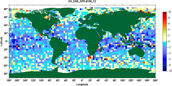
- Variance of the WTC field;
- White noise associated with each WTC data set (required to compute the diagonal elements of the variance-covariance matrix );
- Parameters defining the correlation function: space and time correlation scales;
- Space and time search radii.
2.2. Dataset Description
- valid WTC observations from the on-board MWR, when available as for GFO;
- zenith wet delays (ZWD), WTC equivalent, from GNSS;
- WTC derived from scanning imaging microwave radiometers.
2.2.1. WTC from on-Board MWR
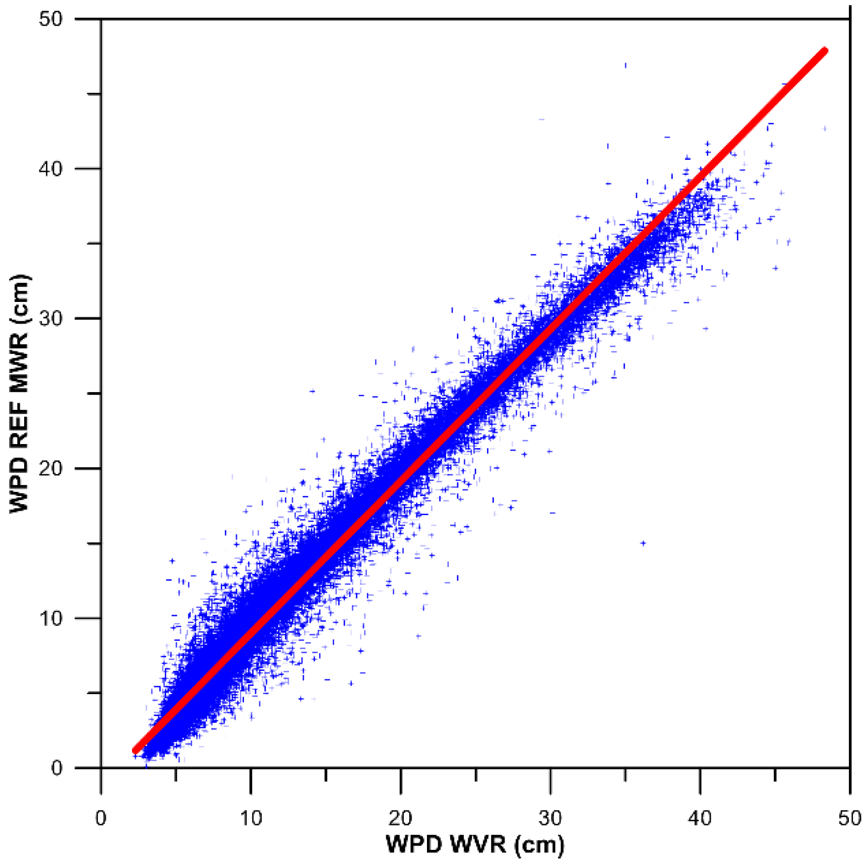
- GFO—Water Vapour Radiometer (WVR) dataset, available in RADS, the most recent version of this product [18];
- TOPEX/Poseidon—Topex Microwave Radiometer (TMR) replacement product [19] available in RADS;
- Jason-1—Jason-1 Microwave Radiometer (JMR) product present in the recently released Geophysical Data Records Version E (GDR-E) available from the Physical Oceanography Distributive Active Archive Center (PODAAC), enhanced near the coast [20];
- Jason-2—Advanced Microwave Radiometer (AMR) GDR-D product, already enhanced near the coast, available in RADS [20].
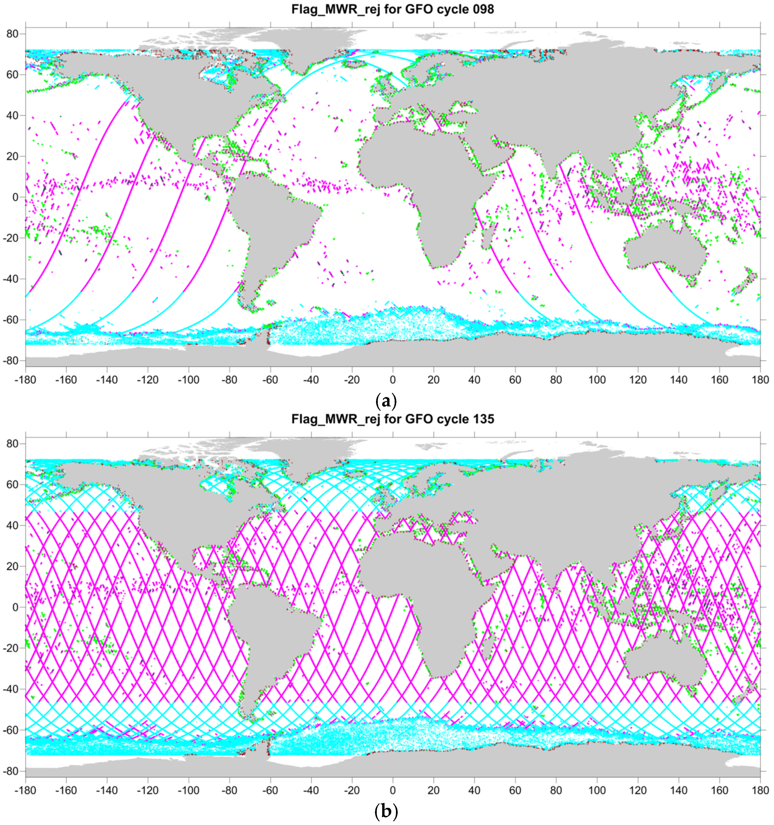
- flag_MWR_rej = 1—if the rad_surf_type flag is 1, usually related with land contamination, but also with instrument problems;
- flag_MWR_rej = 2—if the measurement was acquired at a distance from the coast less than a given threshold, e.g., 30 km for GFO and TOPEX/Poseidon; 20 km for Jason-1 and 15 km for Jason-2;
- flag_MWR_rej = 3—if the ice_flag is 1, indicating ice contamination. More generally, an invalid point located in the latitude bands |ϕ| > 45° may be flagged as ice even if this is not the actual cause of invalidity;
- flag_MWR_rej = 4—based on statistical parameters, including median filters, function of the differences between MWR and model WTC, not only at the same measurements but also at neighbouring points (related with ice, land, rain or outlier detection);
- flag_MWR_rej = 5—if the MWR WTC is ≥0.0 m or <−0.5 m, usually associated with rain or ice contamination, or instrument failure.
2.2.2. GNSS-Derived WTC
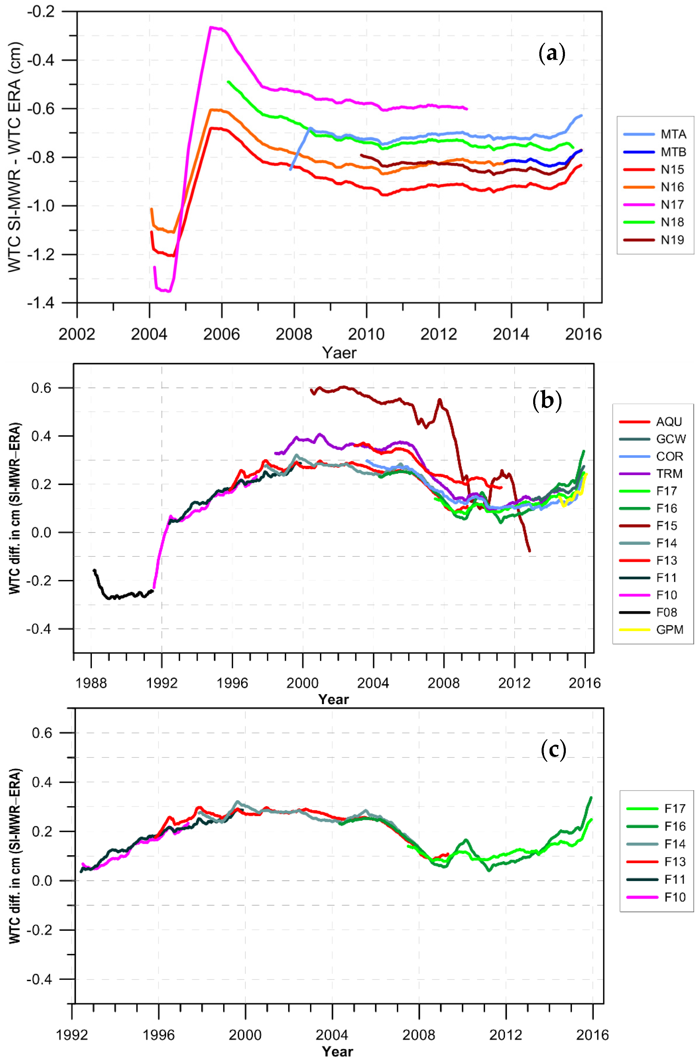
2.2.3. Total Column Water Vapour (TCWV) from SI-MWR
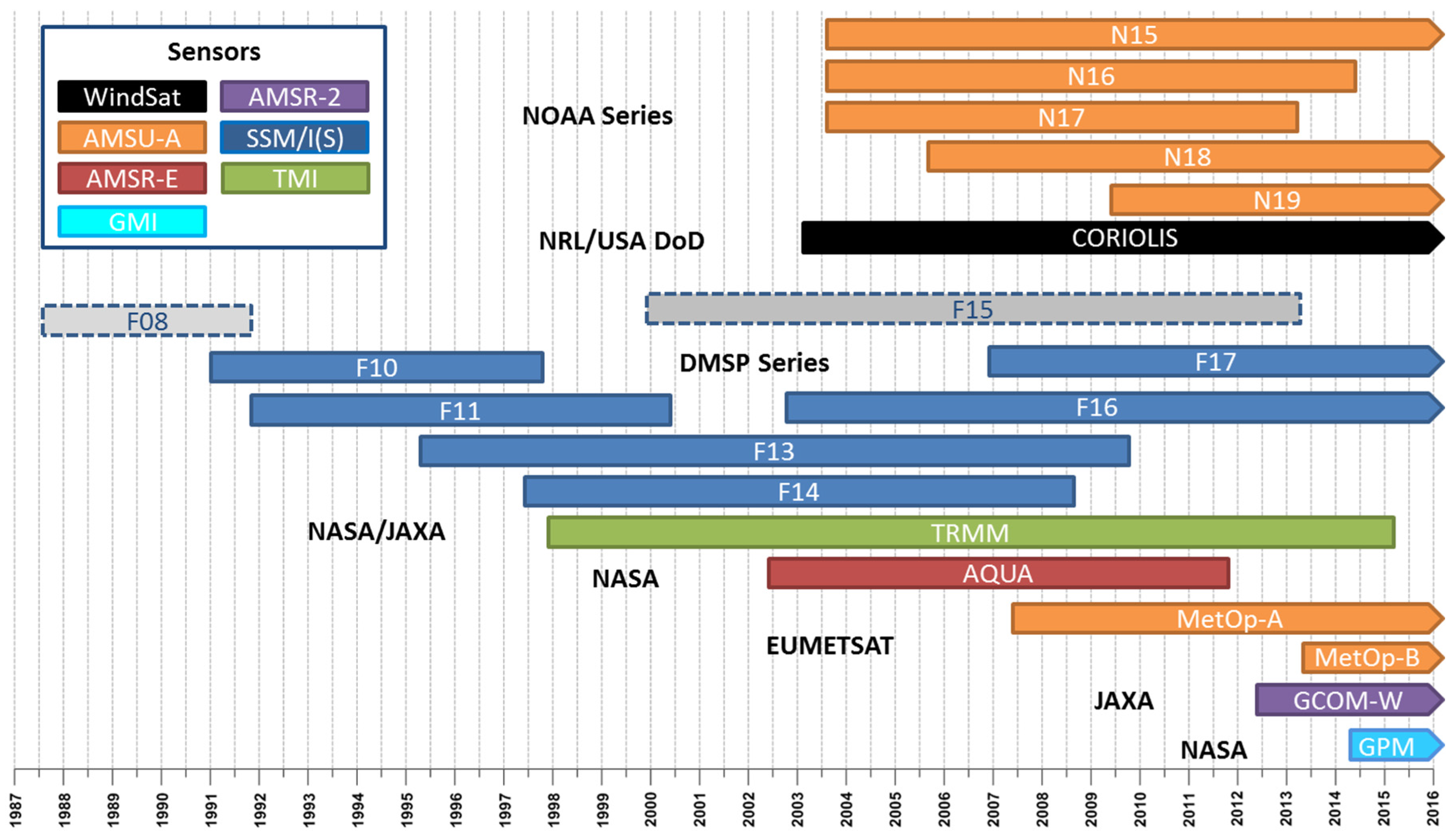
- AMSU-A Level-2 swath products are available, in HDF-EOS2 format, from NOAA CLASS [26] as Microwave Surface and Precipitation Products System (MSPPS) Orbital Global Data products (MSPPS_ORB) for NOAA-15, -16, -17, -18, -19, MetOp-A and MetOp-B.
- Remote Sensing Systems [27] provides gridded products, in binary format, for the following sensors: AMSR-E (AQUA), AMSR-E (GCOM-W1), WindSat (Coriolis), TMI (TRMM), GMI (GPM), SSM/I (DMSP satellites F08, F10, F13, F14, F15) and SSM/IS (F16, F17). Two 0.25° × 0.25° global grids per day are provided for each sensor, one containing the ascending and the other the descending passes. According to RSS information, after August 2006, F15 products are affected by RADCAL beacon interference. For this reason and due to the instabilities shown in this study, F15 data are not being used in the WTC estimations.
2.2.4. Tropospheric Delays from the ECMWF
- sea level pressure (SLP);
- surface temperature (2-m temperature, 2T);
- integrated water vapour (Total Column Water Vapour, TCWV).
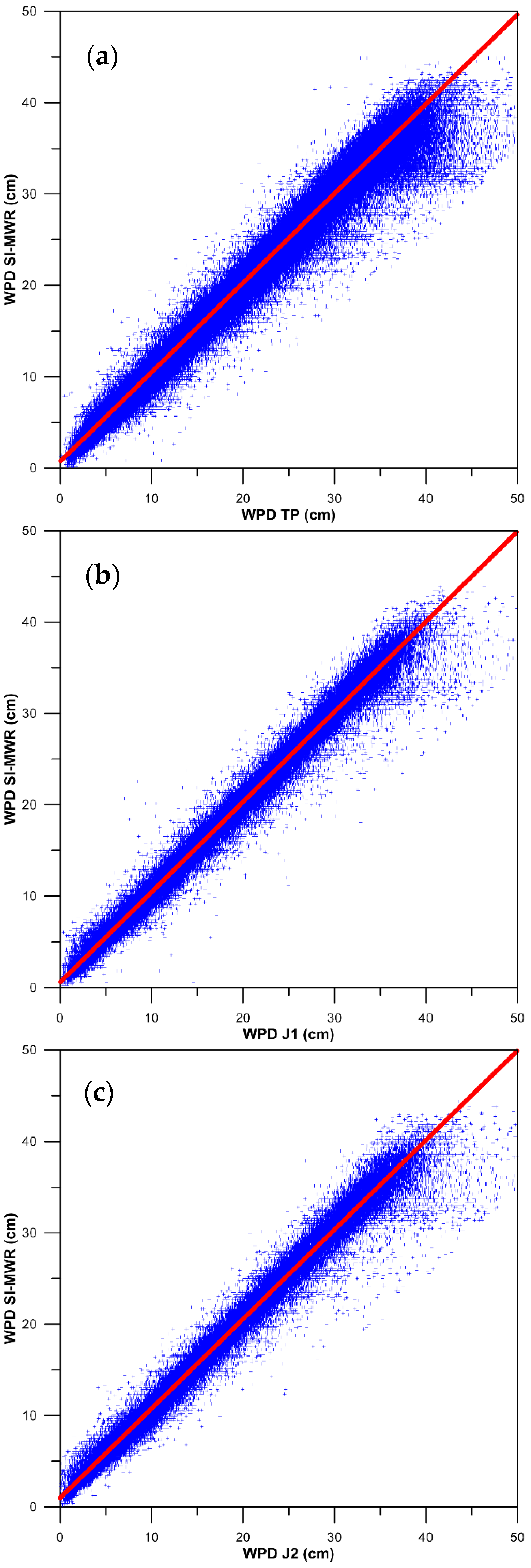
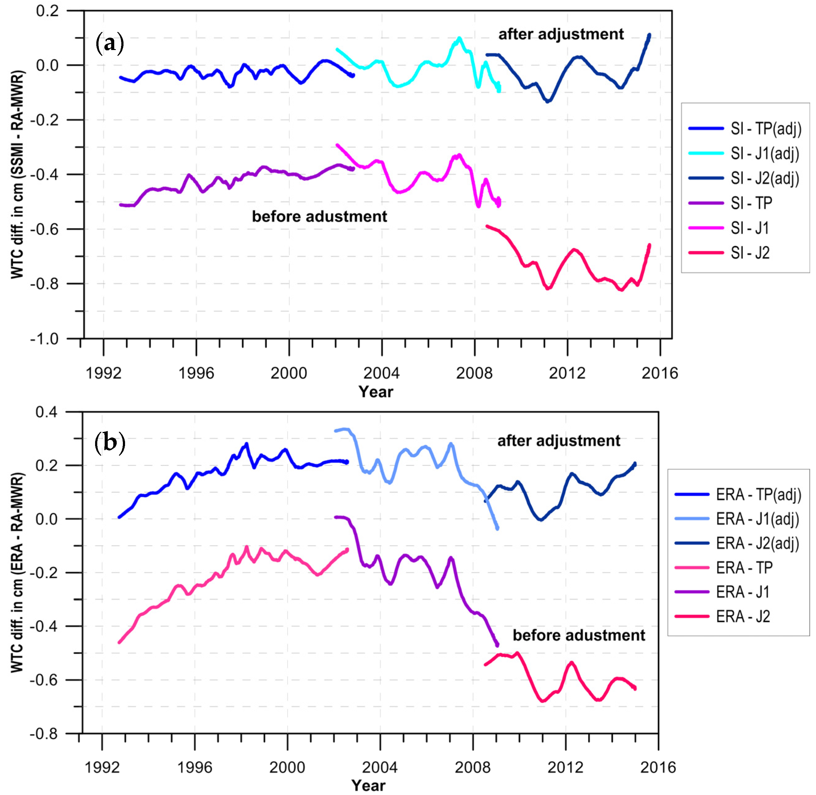
2.3. Sensor Calibration
- Step 1—TOPEX/Poseidon (TP), Jason-1 (J1) and Jason-2 (J2) were calibrated against the SSM/I and SSM/IS sensors on board the “FXX” satellite series;
- Step 2—GFO was calibrated against previously calibrated TP, J1, J2;
- Step 3—remaining SI-MWR were calibrated against previously calibrated TP, J1, J2.
3. GPD+ WTC for CryoSat-2 and GFO
3.1. CryoSat-2
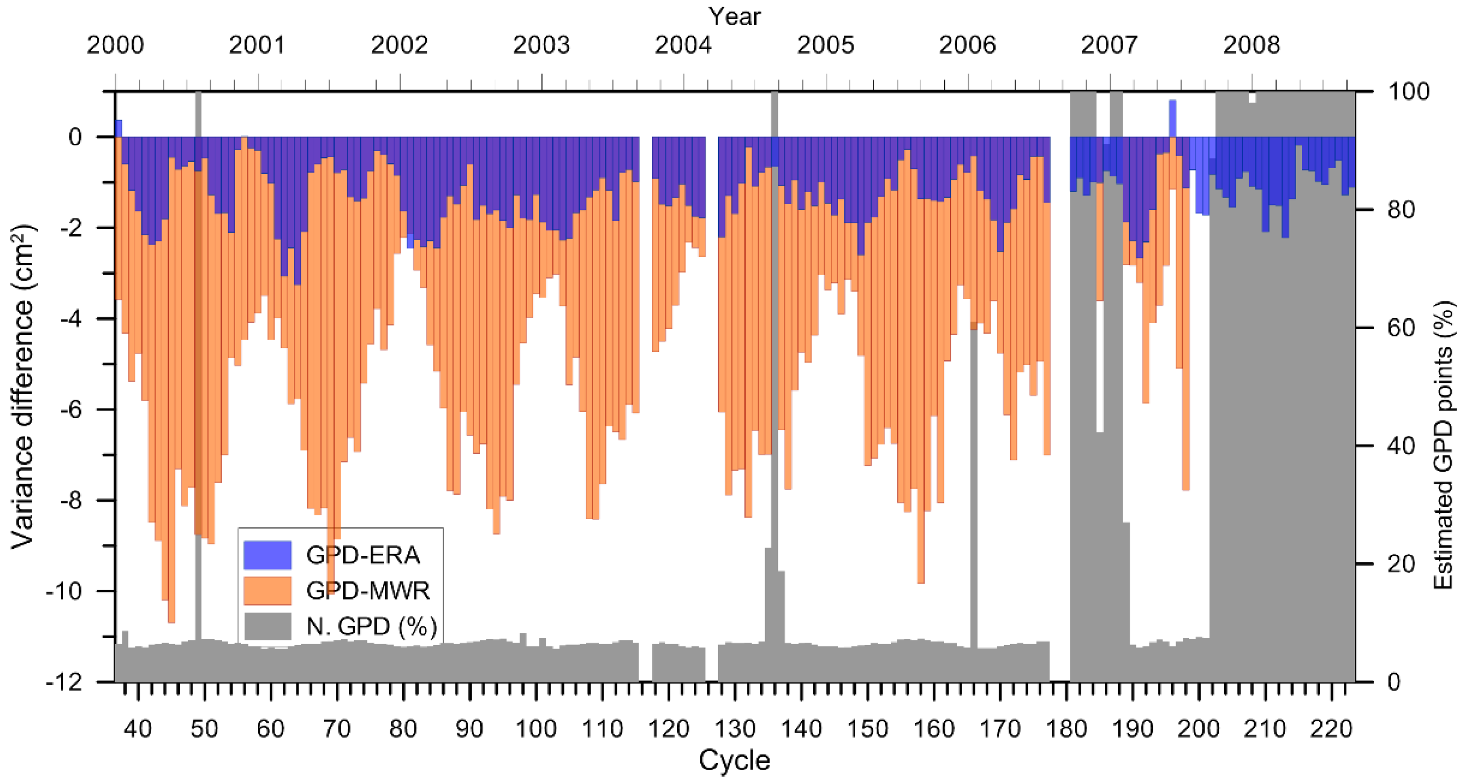
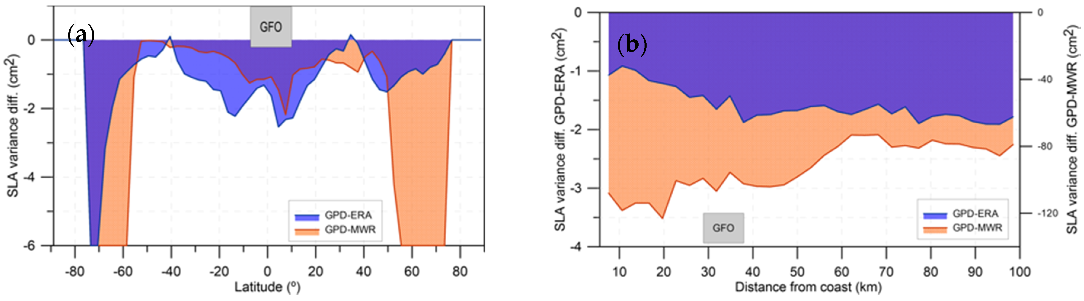
3.2. Geosat Follow-on
4. Discussion and Conclusions
Acknowledgments
Author Contributions
Conflicts of Interest
Abbreviations
| AMR | Advanced Microwave Radiometer |
| CLASS | Comprehensive Large Array-Data Stewardship System |
| CP4O | CryoSat Plus for Oceans |
| CS-2 | CryoSat-2 |
| DMSP | Defense Meteorological Satellite Program |
| ECMWF | European Centre for Medium-Range Weather Forecasts |
| EPN | EUREF Permanent Network |
| ERA | ECMWF ReAnalysis |
| ESA | European Space Agency |
| GDR | Geophysical Data Records |
| GFO | Geosat Follow-On |
| GNSS | Global Navigation Satellite Systems |
| GPD+ | GNSS-derived Path Delay Plus |
| IGS | International GNSS Service |
| J1 | Jason-1 |
| J2 | Jason-2 |
| JMR | Jason-1 Microwave Radiometer |
| LRM | Loe Resolution Mode |
| MWR | MicroWave Radiometer |
| NWM | Numerical Weather Models |
| OA | Objective Analysis |
| POD | Precise Orbit Determination |
| PODAAC | Physical Oceanography Distributive Active Archive Center |
| RADS | Radar Altimeter Database System |
| RSS | Remote Sensing Systems |
| SI-MWR | Scanning Imaging MWR |
| SL_cci | Sea Level Climate Change Initiative |
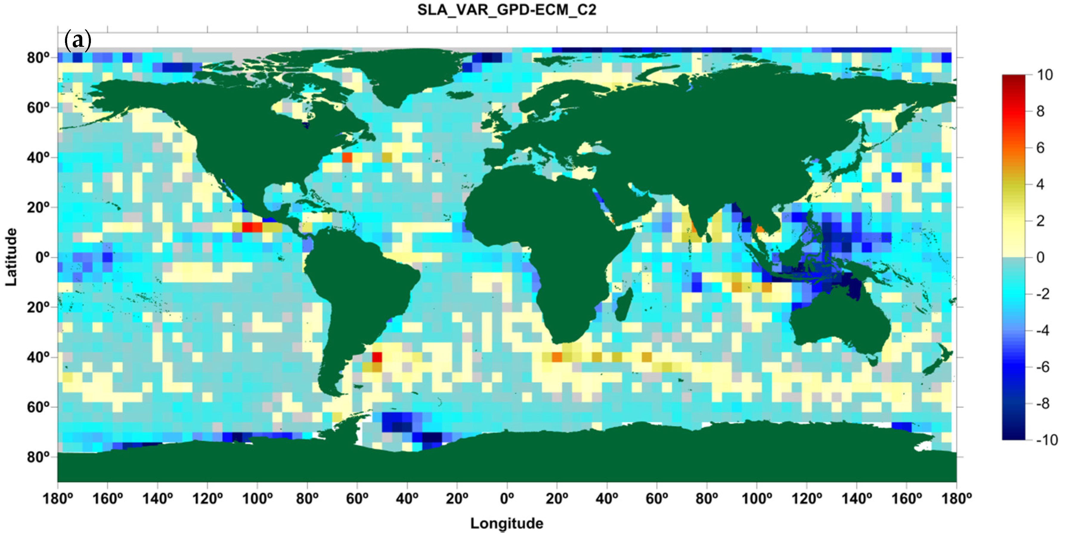
| SLA | Sea Level Anomaly |
| SLP | Sea Level Pressure |
| SSH | Sea Surface Height |
| SSM/I | Special Sensor Microwave Imager |
| SSM/IS | Special Sensor Microwave Imager Sounder |
| T/P | TOPEX/Poseidon |
| TCWV | Total Column Water Vapour |
| TMR | Topex Microwave Radiometer |
| UPorto | University of Porto |
| WTC | Wet Ttropospheric Correction |
| WVR | Water Vapour Radiometer |
| ZHD | Zenith Hydrostatic Delay |
| ZTD | Zenith Total Delays |
| ZWD | Zenith Wet Delay |
References
- Chelton, D.B.; Ries, J.C.; Haines, B.J.; Fu, L.L.; Callahan, P.S. Satellite altimetry. In Satellite Altimetry and Earth Sciences: A Handbook of Techniques and Applications; Fu, L.L., Cazenave, A., Eds.; Academic Press: San Diego, CA, USA, 2001. [Google Scholar]
- Ablain, M.; Cazenave, A.; Larnicol, G.; Balmaseda, M.; Cipollini, P.; Faugere, Y.; Fernandes, M.J.; Henry, O.; Johannessen, J.A.; Knudsen, P.; et al. Improved sea level record over the satellite altimetry era (1993–2010) from the Climate Change Initiative project. Ocean Sci. 2015, 11, 67–82. [Google Scholar] [CrossRef] [Green Version]
- Miller, M.; Buizza, R.; Haseler, J.; Hortal, M.; Janssen, P.; Untch, A. Increased resolution in the ECMWF deterministic and ensemble prediction systems. In ECMWF Newsletter; ECMWF: Reading, UK, 2010. [Google Scholar]
- Dee, D.P.; Uppala, S.M.; Simmons, A.J.; Berrisford, P.; Poli, P.; Kobayashi, S.; Andrae, U.; Balmaseda, M.A.; Balsamo, G.; Bauer, P.; et al. The ERA-Interim reanalysis: Configuration and performance of the data assimilation system. Q. J. R. Meteorol. Soc. 2011, 137, 553–597. [Google Scholar] [CrossRef]
- Cotton, D.; Benveniste, J.; Clarizia, M.-P.; Roca, M.; Gommenginger, C.; Naeije, M.; Labroue, S.; Picot, N.; Fernandes, J.; Andersen, O.; et al. CryoSat plus for oceans: An ESA Project for CryoSat-2 data exploitation over ocean. In Proceedings of the EGU General Assembly, Vienna, Austria, 27 April–2 May 2013.
- Vignudelli, S.; Cipollini, P.; Gommenginger, C.; Snaith, H.M.; Coelho, H.; Fernandes, J.; Gomez-Enri, J.; Martin-Puig, C.; Woodworth, P.; Dinardo, S.; et al. The COASTALT project: Towards an operational use of satellite altimetry in the coastal zone. In Proceedings of the OCEANS 2009 MTS/IEEE Biloxi Conference, Biloxi, MS, USA, 26–29 October 2009.
- Fernandes, M.J.; Lazaro, C.; Nunes, A.L.; Pires, N.; Bastos, L.; Mendes, V.B. GNSS-derived path delay: An approach to compute the wet tropospheric correction for coastal altimetry. IEEE Geosci. Remote Sens. Lett. 2010, 7, 596–600. [Google Scholar] [CrossRef]
- Larnicol, G.; Cazenave, A.; Faugère, Y.; Ablain, M.; Johannessen, J.; Stammer, D.; Timms, G.; Knudsen, P.; Cipolini, P.; Roca, M.; et al. ESA sea level climate change initiative. In Proceedings of the 20 Years of Progress in Radar Altimetry Symposium, Venice, Italy, 24–29 September 2012.
- Fernandes, M.J.; Lazaro, C.; Ablain, M.; Pires, N. Improved wet path delays for all ESA and reference altimetric missions. Remote Sens. Environ. 2015, 169, 50–74. [Google Scholar] [CrossRef]
- Stum, J.; Sicard, P.; Carrere, L.; Lambin, J. Using objective analysis of scanning radiometer measurements to compute the water vapor path delay for altimetry. IEEE Trans. Geosci. Remote Sens. 2011, 49, 3211–3224. [Google Scholar] [CrossRef]
- Fernandes, M.J.; Nunes, A.L.; Lazaro, C. Analysis and inter-calibration of wet path delay datasets to compute the wet tropospheric correction for CryoSat-2 over ocean. Remote Sens. 2013, 5, 4977–5005. [Google Scholar] [CrossRef]
- Bretherton, F.P.; Davis, R.E.; Fandry, C.B. A technique for objective analysis and design of oceanographic experiment applied to MODE-73. Deep-Sea Res. 1976, 23, 559–582. [Google Scholar] [CrossRef]
- Schüler, J. On Ground-Based GPS Tropospheric Delay Estimation; Universität der Bundeswehr: München, Germany, 2001. [Google Scholar]
- Leeuwenburgh, O. Covariance modelling for merging of multi-sensor ocean surface data. In Methods and Applications of Inversion; Hansen, P.C., Jacobsen, B.H., Mosegaard, K., Eds.; Springer: Heidelberg, Germany, 2000; pp. 203–216. [Google Scholar]
- Legeais, J.F.; Ablain, M.; Thao, S. Evaluation of wet troposphere path delays from atmospheric reanalyses and radiometers and their impact on the altimeter sea level. Ocean Sci. 2014, 10, 893–905. [Google Scholar] [CrossRef]
- Fernandes, M.J.; Lazaro, C.; Nunes, A.L.; Scharroo, R. Atmospheric corrections for altimetry studies over inland water. Remote Sens. 2014, 6, 4952–4997. [Google Scholar] [CrossRef]
- Bosser, P.; Bock, O.; Pelon, J.; Thom, C. An improved mean-gravity model for GPS hydrostatic delay calibration. IEEE Geosci. Remote Sens. Lett. 2007, 4, 3–7. [Google Scholar] [CrossRef]
- Scharroo, R.; Leuliette, E.W.; Lillibridge, J.L.; Byrne, D.; Naeije, M.C.; Mitchum, G.T. RADS: Consistent multi-mission products. In Proceedings of the 20 Years of Progress in Radar Altimetry Symposium, Venice, Italy, 20–28 September 2012.
- Brown, S. Topex Microwave Radiometer Replacement. Available online: http://podaac.jpl.nasa.gov/dataset/TOPEX_L2_OST_TMR_Replacement (accessed on 16 October 2016).
- Brown, S. A novel near-land radiometer wet path-delay retrieval algorithm: Application to the Jason-2/OSTM advanced microwave radiometer. IEEE Trans. Geosci. Remote Sens. 2010, 48, 1986–1992. [Google Scholar] [CrossRef]
- Kouba, J. Implementation and testing of the gridded Vienna Mapping Function 1 (VMF1). J. Geod. 2008, 82, 193–205. [Google Scholar] [CrossRef]
- Davis, J.L.; Herring, T.A.; Shapiro, I.I.; Rogers, A.E.E.; Elgered, G. Geodesy by radio interferometry—Effects of atmospheric modeling errors on estimates of baseline length. Radio Sci. 1985, 20, 1593–1607. [Google Scholar] [CrossRef]
- Fernandes, M.J.; Pires, N.; Lazaro, C.; Nunes, A.L. Tropospheric delays from GNSS for application in coastal altimetry. Adv. Space Res. 2013, 51, 1352–1368. [Google Scholar] [CrossRef]
- Wentz, F.J. A well-calibrated ocean algorithm for special sensor microwave/imager. J. Geophys. Res. Oceans 1997, 102, 8703–8718. [Google Scholar] [CrossRef]
- Wentz, F.J. SSM/I Version-7 Calibration Report; 011012; Remote Sensing Systems: Santa Rosa, CA, USA, 2013. [Google Scholar]
- NOAA. Comprehensive Large Array-data Stewardship System (CLASS). Available online: http://www.class.ngdc.noaa.gov (accessed on 16 October 2016).
- Remote Sensing Systems (RSS). In Remote Sensing Systems. Available online: http://www.ssmi.com/ssmi/ssmi_browse.html (accessed on 16 October 2016).
- Fernandes, M.J.; Lázaro, C. GPD+ wet tropospheric corrections - impacts on mean sea level. IEEE Trans. Geosc. Remote Sens. 2016. Submitting. [Google Scholar]


| Satellite | Sensor | Height (km) | Inclination (°) | Period (min) | Sun-Synch. Orbit | Data Availability for Cryosat-2 |
|---|---|---|---|---|---|---|
| CryoSat-2 | - | 717 | 92.0 | 93.2 | No | since April 2010 |
| GFO | WVR | 800 | 108.0 | 100.0 | No | February 1998–September 2002 |
| DMSP-F08 | SSM/I | 856 | 98.8 | 102.1 | Yes | June 1987–December 1991 |
| DMSP-F10 | SSM/I | 785 | 98.8 | 100.5 | Yes | December 1990–November 1997 |
| DMSP-F11 | SSM/I | 860 | 98.8 | 101.9 | Yes | November 1991–May 2000 |
| DMSP-F13 | SSM/I | 850 | 98.8 | 102.0 | Yes | March 1995–November 2009 |
| DMSP-F14 | SSM/I | 852 | 98.8 | 102.0 | Yes | May 1997–August 2008 |
| DMSP-F15 | SSM/I | 850 | 98.8 | 102.0 | Yes | December 1999–May 2013 |
| DMSP-F16 | SSM/IS | 845 | 98.9 | 101.8 | Yes | since October 2003 |
| DMSP-F17 | SSM/IS | 850 | 98.8 | 102.0 | Yes | since December 2006 |
| NOAA-15 | AMSU-A | 807 | 98.5 | 101.1 | Yes | since July 2003 |
| NOAA-16 | AMSU-A | 849 | 99.0 | 102.1 | Yes | July 2003–June 2014 |
| NOAA-17 | AMSU-A | 810 | 98.7 | 101.2 | Yes | July 2003–April 2013 |
| NOAA-18 | AMSU-A | 854 | 98.7 | 102.1 | Yes | since August 2005 |
| NOAA-19 | AMSU-A | 870 | 98.7 | 102.1 | Yes | since May 2009 |
| MetOp-A | AMSU-A | 817 | 98.7 | 101.4 | Yes | since May 2007 |
| MetOp-B | AMSU-A | 817 | 98.7 | 101.4 | Yes | since April 2013 |
| AQUA | AMSR-E | 705 | 98.0 | 99.0 | Yes | May 2002–October 2011 |
| GCOM-W1 | AMSR-2 | 700 | 98.2 | 98.0 | Yes | since May 2012 |
| TRMM | TMI | 402 | 35.0 | 93.0 | No | December 1997–March 2015 |
| Coriolis | WindSat | 830 | 98.8 | 101.6 | Yes | since February 2003 |
| GPM | GMI | 407 | 65.0 | 93.0 | No | since March 2014 |
| Satellite | Offset | Scale Factor (cm) | Trend (mm/Year) | RMS after Adjustment (cm) |
|---|---|---|---|---|
| TP | −0.8053 | 0.9781 | 0.1500 | 0.913 |
| J1 | −0.5085 | 0.9872 | −0.0492 | 0.838 |
| J2 | −0.6246 | 0.9798 | −0.1775 | 0.922 |
| GFO | 0.4711 | 0.9932 | 0.0153 | 1.096 |
| NOAA-15 | −0.4523 | 1.0173 | −0.0906 | 1.125 |
| NOAA-16 | −0.5116 | 1.0122 | −0.0963 | 1.007 |
| NOAA-17 | −0.9249 | 0.9880 | 0.1027 | 0.979 |
| NOAA-18 | −0.3275 | 1.0109 | −0.1111 | 1.019 |
| NOAA-19 | −0.1160 | 1.0100 | −0.2524 | 1.012 |
| MetOp-A | −0.5271 | 1.0017 | −0.1052 | 1.007 |
| MetOp B | −1.0008 | 1.0006 | - | 1.110 |
| AQUA | −0.0613 | 0.9909 | 0.0149 | 0.812 |
| GCOM-W1 | −0.1411 | 0.9917 | - | 0.719 |
| Coriolis | 0.0340 | 0.9899 | −0.0968 | 0.779 |
| TRMM | 0.0204 | 0.9964 | −0.0235 | 1.001 |
| GPM | −0.2622 | 0.9875 | - | 0.771 |
© 2016 by the authors; licensee MDPI, Basel, Switzerland. This article is an open access article distributed under the terms and conditions of the Creative Commons Attribution (CC-BY) license (http://creativecommons.org/licenses/by/4.0/).
Share and Cite
Fernandes, M.J.; Lázaro, C. GPD+ Wet Tropospheric Corrections for CryoSat-2 and GFO Altimetry Missions. Remote Sens. 2016, 8, 851. https://doi.org/10.3390/rs8100851
Fernandes MJ, Lázaro C. GPD+ Wet Tropospheric Corrections for CryoSat-2 and GFO Altimetry Missions. Remote Sensing. 2016; 8(10):851. https://doi.org/10.3390/rs8100851
Chicago/Turabian StyleFernandes, M. Joana, and Clara Lázaro. 2016. "GPD+ Wet Tropospheric Corrections for CryoSat-2 and GFO Altimetry Missions" Remote Sensing 8, no. 10: 851. https://doi.org/10.3390/rs8100851