A New Neighboring Pixels Method for Reducing Aerosol Effects on the NDVI Images

Abstract

A new algorithm was developed in this research to minimize aerosol effects on the normalized difference vegetation index (NDVI). Simulation results show that in red-NIR reflectance space, variations in red and NIR channels to aerosol optical depth (AOD) follow a specific pattern. Based on this rational, the apparent reflectance in these two bands of neighboring pixels were used to reduce aerosol effects on NDVI values of the central pixel. We call this method the neighboring pixels (NP) algorithm. Validation was performed over vegetated regions in the border area between China and Russia using Landsat 8 Operational Land Imager (OLI) imagery. Results reveal good agreement between the aerosol corrected NDVI using our algorithm and that derived from the Landsat 8 surface reflectance products. The accuracy is related to the gradient of NDVI variation. This algorithm can achieve high accuracy in homogeneous forest or cropland with the root mean square error (RMSE) being equal to 0.046 and 0.049, respectively. This algorithm can also be applied to atmospheric correction and does not require any information about atmospheric conditions. The use of the moving window analysis technique reduces errors caused by the spatial heterogeneity of aerosols. Detections of regions with homogeneous NDVI are the primary sources of biases. This new method is operational and can prove useful at different aerosol concentration levels. In the future, this approach may also be used to examine other indexes composed of bands attenuated by noises in remote sensing.

1. Introduction

The normalized difference vegetation index (NDVI) derived from remote sensing data has achieved great success in monitoring global vegetation variations. However, the observation of NDVI by optical remote sensing is always disturbed by atmosphere among which aerosols are some of the most active components [1,2,3]. Molecular scattering and absorption and water vapor absorption are relatively easy to correct because their concentrations are quite stable in both spatial and temporal dimensions while aerosol loading is highly variable over both time and space [4]. For pixels with vegetation, the observed NDVI signal drops after aerosol effects and leads to an underestimation of the amount of vegetation at surface [5]. Thus, aerosol correction is of great importance in regions with high aerosol loadings or in biomass burning conditions before vegetation monitoring with NDVI.

There are essentially two methods to minimize aerosol effects on vegetation indices (VIs): The first method involves retrieving the ambient aerosol optical depth (AOD) as an input parameter into the atmospheric correction algorithm to generate surface reflectance product. Approaches to remote sensing of aerosols over land include the Dark-target (DT) aerosol retrieval algorithm [6,7], the deep blue algorithm [8,9,10] and the structure function method [11]. The DT algorithm derives aerosol properties including AOD over land and ocean and has been successfully applied to dark targets in multispectral data such as the moderate-resolution imaging spectroradiometer (MODIS) [12,13,14] and Landsat Thematic Mapper (TM) data [4,15] assisted by the short-wave infrared (SWIR) band (2100 nm). The deep blue algorithm uses the blue band (412 nm) to retrieve aerosol properties and can be applied over both dark and bright surfaces. The structure function method is based on temporal and spatial information contained in remote sensing data and has been validated for the Sahara region based on the TM data. Aerosol retrieval algorithms were also used to retrieve AOD over land using time-series satellite data, multi-angle data, spatial correlation method [1,2,16] and the Simplified Aerosol Algorithm (SARA) [17,18,19].

The second method involves defining a new index that is less sensitive to atmospheric effects. Kaufman and Tanré used the blue band to correct the aerosol effects on the red band and developed the atmospherically resistant vegetation index (ARVI) [20]. In the ARVI, the value of correction coefficient γ depends on the aerosol type. Later, the theory of ARVI was incorporated into the combined soil adjusted and atmospherically resistant vegetation index (SARVI) [20], modified NDVI (MNDVI) [21] and enhanced vegetation index (EVI) [5,22] as a part responsible for eliminating aerosol effects based on two coefficients of the aerosol resistance term C₁ and C₂. VIs using the blue band to minimize atmospheric influences are limited to the sensor designed with a blue band. Jiang et al. developed a two-band enhanced vegetation index (EVI2) without a blue band and can achieve high accuracy when atmospheric influences are insignificant [23]. Karnieli et al. put forward a new aerosol free vegetation index AFRI wherein the red band is replaced by the shortwave infrared (SWIR) spectral bands around 1.6 and 2.1 μm [24].

Existing methods for remote sensing of aerosol or constructing aerosol resistant VIs are mainly based on the wavelength dependency of aerosol effects [22]. The apparent reflectance (also called top-of-atmosphere reflectance) is more sensitive to AOD in the blue (0.47 μm) and red band (0.65 μm) and is less sensitive in the SWIR band (2.13 μm). They were thus used to construct aerosol indices [25]. Aerosol resistant VIs such as AFRI and ARVI and aerosol retrieval algorithms of the DT method were all skillfully developed based on the polarization of aerosol effects on different bands and have achieved very good results. However, it should be noted that they also suffer from many limitations. For instance, aerosol free vegetation indices can introduce larger errors when improper coefficients values (e.g., γ, C₁, C₂ and ρ_SWIR/ρ_red) were used. The DT algorithm relies too much on the targets being dark and is obstructed when aerosols distribution is spatially heterogeneous [4,26]. The deep blue algorithm is strongly dependent on the precalculated surface reflectance database [10,27].

The aerosol influences change with wavelength. For a specific wavelength, there is a corresponding value of the critical surface reflectance with almost no influence of the aerosols. Reflectance lower or larger than the critical reflectance value responses oppositely to aerosol effects [28]. Based on this theory, the aim of this study is to propose another approach to deriving aerosol corrected NDVI and demonstrate the application of this image-based algorithm in the Landsat Data Continuity Mission (LDCM), Landsat 8 Operational Land imager (OLI) data. This method which will be called hereafter the neighboring pixels (NP) algorithm has the potential to evaluate the atmospheric corrected NDVI of the central pixel from apparent reflectance in the red and near infrared (NIR) band of neighboring pixels, especially achieving high accuracy in homogeneous forest or patches of cropland. In this paper, our proposed algorithm is described in detail in Section 2. In Section 3, experiments using the proposed algorithm are presented. Factors influencing algorithm accuracy and a discussion about them are presented in Section 4.

2. Methods

2.1. Vegetation Isolines Simulations Using the 6S Radiative Transfer Code

Huete et al. (1985) and Huete and Jackson (1987) found that observed vegetation isolines (constant vegetation amount) at various canopy densities for cotton and grass with different soil backgrounds in red-NIR wavelength space converge at one point located at the third quadrant rather than at the origin [29,30]. They added a constant, l, to the red and NIR reflectance values and proposed a new VI called the soil-adjusted vegetation index (SAVI). Soil backgrounds influence the NDVI by keeping canopies of the same NDVI but with different soil moisture backgrounds away from the NDVI isoline. Assuming that the fraction of vegetation cover does not change over a short period of time but is disturbed by the soil background, the observed NDVI changes. Similarly, aerosols in the atmosphere cause the observed NDVI to deviate from the surface true NDVI by affecting the observed reflectance in the red and NIR bands that compose NDVI. Thus, it is necessary to determine how aerosols affect the apparent reflectance values.

A simulation of aerosol effects on apparent reflectance in the red (0.662 μm) and NIR (0.835 μm) bands was performed using the Second Simulation of the Satellite Signal in the Solar Spectrum (6S) radiative transfer model. 6S has been extensively validated, and the accuracy of simulated top-of-atmosphere (TOA) reflectance falls within 0.5% that has met the standard RT code accuracy requirement [31,32]. The zenith and azimuth angles for the satellite were both set to be 0°, and the zenith and azimuth angles for the sun were 21° and 142°, respectively. The mid-latitude summer model was selected. The simulation was performed across the band with a constant filter function of 1.0. The surface was assumed to be Lambertian. Studies on uncertainties of the atmospheric correction by 6S show that errors due to uncertainties in aerosol model assumptions dominate other sources such as atmospheric parameters and calibration uncertainties [33]. Aerosol model selection has strong effects on atmospheric correction results [34,35,36]. In 6S, pre-defined standard aerosol models include continental, maritime, urban, user’s model and three new models (biomass burning smoke, background desert and stratospheric models) [37]. In this paper, continental, urban, biomass burning and maritime models were used for simulation, as these aerosol types are typical in continents characterized by large areas of vegetation.

Simulations were performed on apparent reflectance in the red and NIR bands for various coverage fractions of four vegetation types with different AOD conditions at 550 nm. The four vegetation types (grass, shrub, arbor and forest) naturally represent almost all vegetation types. The following six vegetation fractions were used: 0.25, 1/3, 0.5, 2/3, 0.75 and 1. The AOD values at 550 nm are the same for the red and NIR band and are dependent on aerosol types. For continental, urban and maritime aerosol models, AOD variations were defined as 0.0001, 0.25, 0.5, 1.0, 1.5 and 1.95. In areas characterized by biomass burning, large quantities of smoke aerosols at high optical depths are produced and AOD at 550 nm can extend up to a value of 2 [38]. Thus, AOD variations were defined as 2, 2.1, 2.2, 2.3, 2.4, 2.5 and 2.6 for the simulation. The surface reflectance values for soil and vegetation are reported in

Table 1. Reflectance of typical soil and vegetation in the red (0.662 μm) and NIR (0.835 μm) bands [20,39].

Surface Cover	R0	N0
Soil	0.190	0.243
Grass	0.052	0.660
Manzanita	0.086	0.370
Trembling Aspen	0.026	0.291
Forest	0.016	0.210

. The hybrid reflectance value is treated as the coverage weighted linear combination of the reflectance of soil and vegetation.

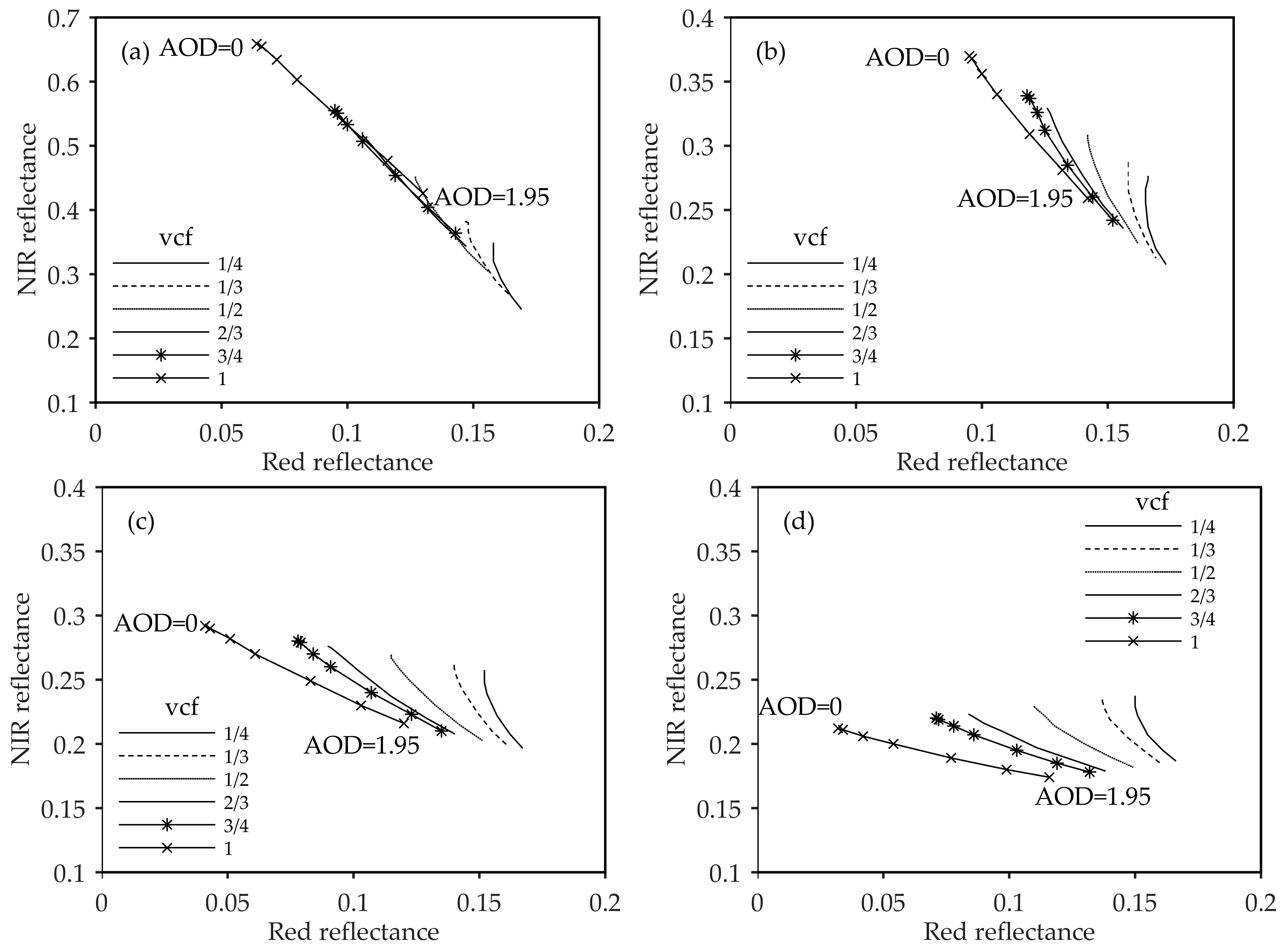
Simulated apparent reflectance for the red (0.662 μm) vs. NIR (0.835 μm) channel as a function of AOD and vegetation coverage fraction of four vegetation types are shown in Figure 1. The values of AOD range from 0.0001 to 1.95 under the continental aerosol type defined in 6S model. Points denoted by the same label in each panel (vegetation spectral isoline) share the same surface reflectance but are fluctuated by different aerosol optical depths. Apparent reflectance in the red band increases as AOD increases while apparent reflectance in the NIR band decreases as AOD increases for hybrid surface reflectivity values in this case. For low surface reflectance in the red band (p < 0.17 as simulation results), net aerosol effects on reflectance are typically characterized by an increase in the detected signal strength. For higher surface reflectance (p > 0.12) in the NIR band, aerosols weaken the signal. For all green vegetation and many soil types, the scattering of signal is more than absorption in the red band while the opposite trend is found in the NIR band. The aerosol degrades NDVI value by reducing the contrast between the red and NIR reflected energies [5]. These findings are almost consistent with the research by Kaufman [20,40].

In Figure 1, it also shows that the slope between reflectance in red and NIR band becomes smaller as vegetation coverage fraction increases. The apparent NDVI begins to be more sensitive to changes in aerosol optical depth for higher vegetation coverage fractions. Thus, the effects of aerosol optical depth on apparent reflectance NDVI values at the pixel scale are related to the surface reflectance which are determined by vegetation coverage fractions in the same panel and different vegetation types represented by four panels in Figure 1. After fitting each vegetation isoline, it could be deduced that these isolines approximately converge at one point.

To find reasons for this phenomenon, relationships between surface reflectance in the red (0.662 μm) and NIR (0.835 μm) band and sensitivity of their apparent reflectance to AOD variations were explored from 6S model calculation. Simulation results are shown in

Table 2. Case study of surface reflectance in red (R₀) and NIR (N₀) channels and sensitivity of apparent reflectance (R* and N*) to AOD variations.

R0	ΔR*/ΔAOD	N0	ΔN*/ΔAOD
0.016	0.044	0.210	−0.020
0.026	0.041	0.291	−0.040
0.045	0.036	0.293	−0.040
0.046	0.036	0.370	−0.058
0.052	0.034	0.380	−0.061
0.086	0.025	0.660	−0.122

. It reveals that for different surface reflectivity values in red and NIR band (R₀, N₀), the sensitivity of apparent reflectance (R*, N*) to aerosol optical depth (ΔR*/ΔAOD, ΔN*/ΔAOD) is different. As AOD increases, aerosols can scatter more photons into the sensor but at the same time increase the signal absorbed by aerosol particles [41]. This combined effect on the detected signal is a result of compensation between path radiance that increases the observed signal and transmittance that decreases the signal [20]. The reflectivity in the red channel is low and the scattering components weigh more. As surface reflectance increases in the red channel, apparent reflectance tends to lose sensitivity to AOD variations. This is attributable to the fact that, in brighter surfaces (high reflectance), high surface reflectivity contributes considerably to apparent reflectance causing apparent reflectance to lose sensitivity to the variation of AOD. In contrast, for the NIR channel, as surface reflectance increases, apparent reflectance becomes more sensitive to AOD variations. Optical effects on the NIR band are more significant for brighter surfaces. This is because, for the NIR band, atmospheric transmission plays a more important role in apparent reflectance. Thus, although the aerosol free reflectances from densely vegetated surfaces to sparsely vegetated areas are different, their responses to aerosol effects are different as well causing apparent reflectance to gradually become similar.

The relationship between surface reflectance and sensitivity of its apparent reflectance to AOD variations was quantitatively investigated based on the data in Table 2. When AOD variation is the same for the red and NIR band, ratio of the apparent reflectance variation in the red band to that in the NIR band can be expressed as Equation (1). Value of ΔN*/ΔR* is equal to the slope of vegetation spectral isoline (k) shown in Figure 1. This formula indicates that for an arbitrary level of partial vegetation cover, its vegetation spectral isoline in relation to AOD is likely to pass through point (r, n). Point (r, n) is the convergence point of extended vegetation spectral isolines for different vegetation cover fractions and different vegetation species. In this case, the convergence point is approximate to point (0.2, 0.1). The location of this convergence point in red-NIR reflectance space is related to parameter r and n, which is dependent on aerosol types and wavelengths for simulation.

$$k=\frac{\Delta N*}{\Delta R*}=\frac{N_0-n}{R_0-r}$$

(1)

where k is the slope of vegetation spectral isoline in Figure 1. ΔR* and ΔN* are variations of apparent reflectance in the red and NIR band, respectively. N₀ and R₀ are surface reflectance in the red and NIR band, respectively. n and r are constants.

2.2. Derivation of Aerosol Corrected NDVI That Incorporates Neighborhood Information

In Figure 1, variations of simulated apparent NDVI in densely vegetated areas (high vegetation coverage fraction) caused by AOD variation are more significant than those found in sparsely vegetated areas. Results are consistent with previous researches [20,42,43]. For dark target and bright target of the same NDVI, Goward et al. [44] found that NDVI variation for dark targets is larger than that for bright targets caused by the same reflectance errors. It indicates that NDVI of dark target is more sensitive to reflectance variation. The atmosphere-induced NDVI degradation for a specific canopy is greater for increasing atmospheric turbidities [3]. Under the same aerosol concentrations, differences between NDVI degradation of different vegetation covered pixels depend on aerosol free NDVI (represented by different vegetation cover fractions and different vegetation species) and canopy brightness (determined by its surface reflectance in red and NIR band (R₀, N₀)). NDVI free of aerosol effects can be surface reflectance NDVI or NDVI that is only contaminated by atmospheric molecular scattering and water absorption. In this section, aerosol free NDVI was used uniformly unless particularly specified.

Thus, NDVI variations are related to AOD, brightness of targets f (R₀, N₀) and aerosol free NDVI (NDVI₀). This relationship could be described in Equation (2). For objects with higher aerosol free NDVI and lower brightness values, aerosol-induced NDVI degradations are larger. Thus, even though the spatial distribution of AOD is homogeneous, NDVI variations for different pixels are still different. Due to spatial heterogeneities of aerosols, the surface reflectance NDVI value cannot be determined without access to aerosol content data. Other solutions need to be found to solve this ill-posed problem.

$$\Delta NDVI=f(AOD,NDV{I}_0，\sqrt{{R_0}^2+{N_0}^2})$$

(2)

Two partial canopies with an equal aerosol free NDVI value were assumed. Aerosol free reflectance in red and NIR band of these two canopies are denoted by (R₁₀, N₁₀) and (R₂₀, N₂₀), respectively. Since the aerosol free NDVI was assumed to be the same for these two canopies, the slope of the line connecting them equals the slope of the aerosol free NDVI isoline (as shown in Equation (3)) in red-NIR reflectance space. If the sky were to become hazier and AOD variations for the two canopies were to remain similar, the slope of the line connecting their apparent reflectance was expressed as Equation (4). Based on the continental aerosol model simulation results, a₁ is approximately equal to a₂. Thus, k′ is equal to k. This means that the slope of line connecting two canopies’ reflectance is invariant to AOD variations (k′ = k) which could help us develop an algorithm to reduce the aerosol effects on NDVI values. The apparent reflectance of at least two pixels with a similar aerosol free NDVI can be used to derive the slope value of k′. Then, the estimated value of the aerosol corrected NDVI (NDVI′) could be derived from k′ based on Equation (5). The same conclusion can be applied to other surface types such as urban impervious surfaces or water.

$$k=\frac{N_{10}}{R_{10}}=\frac{N_{20}}{R_{20}}=\frac{N_{20}-N_{10}}{R_{20}-R_{10}}$$

(3)

$$k\prime =\frac{N_2*-N_1*}{R_2*-R_1*}=\frac{(N_{20}-N_{10})(1+a_2\cdot AOD)}{(R_{20}-R_{10})(1+a_1\cdot AOD)}$$

(4)

where R₁₀, N₁₀, R₂₀ and N₂₀ denote aerosol free reflectance in the red and NIR band for the two pixels covered by partial canopies, respectively. R₁*, N₁*, R₂* and N₂* denote apparent reflectance in the red and NIR bands for the two pixels covered by partial canopies, respectively. Regression coefficients a₁ and a₂ represent the rate of change of apparent reflectance in the red and NIR band as a function of changes in AOD. k indicates the slope of line connecting two canopies’ aerosol free reflectance and k′ indicates the slope of line connecting two canopies’ apparent reflectance.

$$NDVI\prime =1-\frac{2}{1+k\prime }$$

(5)

The spectral dependence of aerosol scattering and absorption are determined by the aerosol type, size and chemical composition features examined [20]. In this study, four 6S standard aerosol models (the continental, urban, biomass burning and maritime models) were used to study how values of parameter a₁ and a₂ vary across these aerosol types. The simulation results are presented in

Table 3. The regression coefficients a₁ and a₂ for four aerosol models.

Aerosol Model	a1	a2	b1	b2
continental	−0.274	−0.224	0.048	0.025
urban	−0.384	−0.356	0.023	0.017
biomass burning	−0.134	−0.105	0.061	0.041
maritime	−0.145	−0.106	0.066	0.055

. The values of a₁ and a₂ are approximately equal in each aerosol model. Thus, the new aerosol correction method can be satisfactorily applied to any one of these four models. The difference between values of a₁ and a₂ is one of the reasons for uncertainties in aerosol correction.

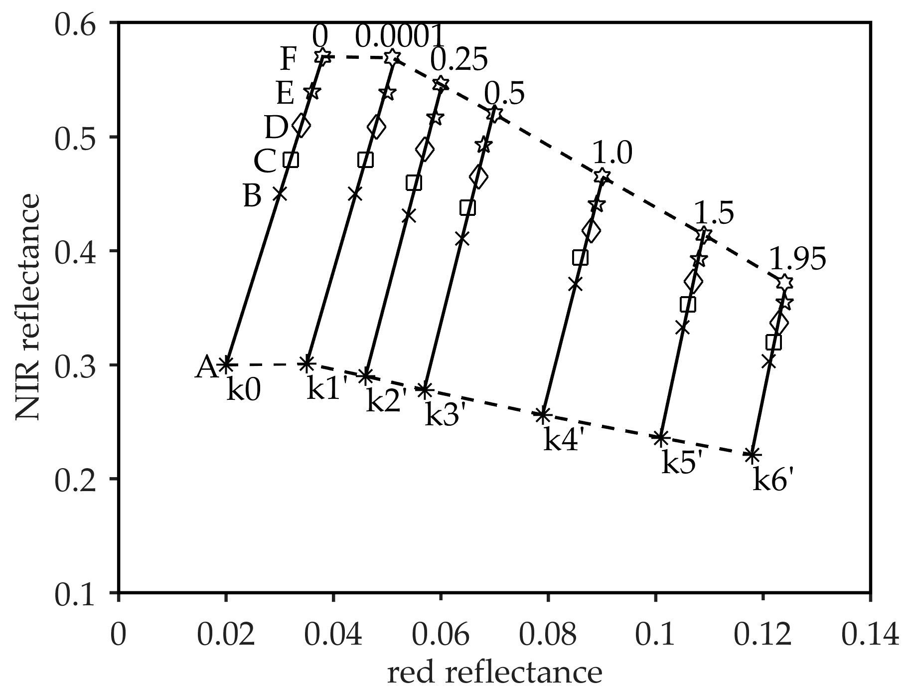
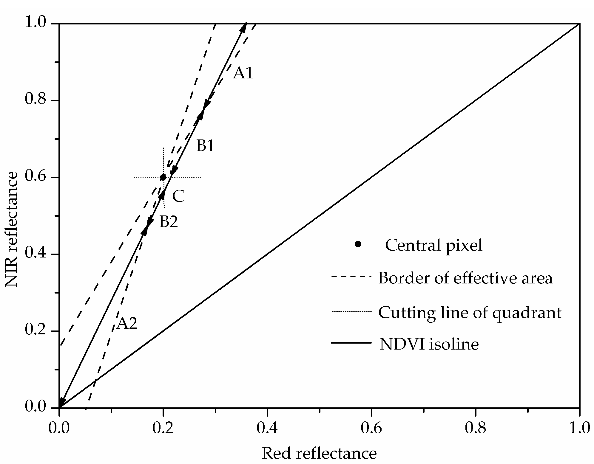
To illustrate what is mentioned above, six partial canopies (A–F) in clear sky conditions are assumed in Figure 2. These six canopies have the same aerosol free NDVI (surface true NDVI or NDVI corrected for molecular scattering and water vapor absorption). In this experiment, AOD varies (0.0001, 0.25, 0.5, 1.0, 1.5 and 1.95) and is assumed to remain the same in all canopies during each phase. Influenced by AOD variations, the apparent reflectance of each canopy changes its value in red-NIR space, and the best fitting straight lines through them in each process could in turn be determined. Value of k0 is the slope of the aerosol free NDVI isoline. The fitted lines with the slope from k1′ to k6′ represent variations of AOD from 0.0001 to 0.25, 0.5, 1.0, 1.5 and 1.95 from the upper-left to the lower-right corner in Figure 2. Lines that connect six canopies’ apparent reflectance are roughly parallel to each other under different AOD conditions. These slope values do not vary considerably and their effects on final NDVI values are minor. In this case, a variation in the AOD of 0.1 results in an error of δ (NDVI) ≈ 0.00156 in NDVI.

2.3. Data and Experimental Design

2.3.1. Study Area and Data

The study region is located in the northeastern part of Heilongjiang Province (seen in Figure 3) in China around 48.08°N and 128.76°E and is covered by two path/row Landsat 8 OLI scenes including World Reference System 2 Path 117 and Row 26 and Path 117 and Row 27. The two scenes were both acquired on 9 August 2014. Compared to the MODIS data that are typically used, the spatial resolution of Landsat multispectral data is high enough to generate enough pure pixels to provide us with relatively stable reflectance. Two subdomains were extracted from this region for algorithm validation.

The first sub region is located in the north of study area in the border area between China and Russia around 49.47°N and 128.97°E and covers 3.6 km × 6 km (1300 × 2000 Landsat pixels). According to the provisional Landsat 8 surface reflectance product available from the U.S. Geological Survey, the selected research area is covered with high aerosol loading. The major land cover types in this area include forest, cropland, grassland, natural vegetation and water. The dark area in the lower left corner of the its true-color image consists largely of mixed forest and is relatively spectrally homogeneous. Cropland and grassland almost cover the upper right corner and these areas are spectrally heterogeneous because of cropland ridges and bare soil. The image is provided to illustrate the performance of the proposed method in different vegetation types and is regarded as a test area in the discussion section.

The second sub region is located in the south of study area around 46.84°N and 128.75°E and covers 4.8 km × 4.8 km (1600 × 1600 Landsat pixels). The main vegetation type in this area is forest. The distribution of atmospheric aerosol is heterogeneous from low to high aerosol loading levels. This sub research area was chosen to validate the performance of the proposed algorithm in different aerosol contents.

2.3.2. Experimental Design

A given neighborhood is normally under similar atmospheric effects. It is reasonable to assume that in the neighborhood of a central pixel, brightness varies under constant NDVI. The error caused by this assumption will be discussed in a later portion of this study. Figure 4 presents a flowchart of steps for reducing aerosol effects on NDVI. All processes will be discussed in detail below.

(1)

Pre-processing

Before implementing the correction process, the Landsat OLI digital numbers (DN) must be calibrated to top-of-atmosphere radiance. In mountainous areas, topographic correction is need to reduce the influence of the topography on the signal recorded by optical sensors [45]. Then, corrections for water vapor absorption and molecular scattering using the Fast Line-of-sight Atmospheric Analysis of Spectral Hypercubes (FLAASH) module in ENVI were conducted in advance. In FLAASH, to do atmospheric correction without removing the aerosol effects, the aerosol model and the aerosol retrieval were set to be no aerosol and none, respectively. The initial visibility value was set to be 100 km. The output reflectance (or radiance) data are only contaminated by aerosol effects based on which the proposed algorithm will be conducted. It should be noted that the processes of topographic correction and FLASSH correction are optional.

(2)

Algorithm implementation

The output reflectance (or radiance) data without removing the aerosol effects generated in the step of pre-processing were used to calculate the aerosol corrected NDVI by our algorithm. In a moving window of size n × n, slope values between each neighboring pixel and the central pixel were computed using apparent reflectance in the red and NIR bands, among which pixels contaminated with cloud or with negative slope values were excluded. Then, the average value of all valid neighboring pixels were used to make prediction for the slope value of the central pixel:

$$k{\prime }_i=\frac{1}{n}{\displaystyle \sum _{j=1}^n\frac{N{*}_{ij}-N{*}_i}{R{*}_{ij}-R{*}_i}}$$

(6)

where k′_i is the estimated mean slope value of neighboring pixels around ith target pixel. R^*_ij and N^*_ij are apparent reflectance of jth neighboring pixel in the red and NIR band, respectively. R^*_i and N^*_i are apparent reflectance of ith target pixel in the red and NIR band, respectively. n denotes the number of neighboring pixels which are not cloud-contaminated and are with positive slope values.

The estimated NDVI value was then derived from the estimated mean k′ value:

$$NDVI{\prime }_i=1-\frac{2}{1+k{\prime }_i}$$

(7)

where NDVI′_i is the estimated aerosol corrected NDVI of ith target pixel.

3. Results

3.1. Optimization of Window Size

Results of NP algorithm implemented with multiple window sizes were compared to surface NDVI derived from the Landsat 8 surface reflectance product generated from the L8SR algorithm. The root mean square error (RMSE) and mean absolute difference (MAD) values in

Table 4. Window sizes and responding inversion accuracy.

Window Size	RMSE	MAD	STD
3 × 3	0.091	0.063	0.006
5 × 5	0.064	0.048	0.005
7 × 7	0.067	0.052	0.042
9 × 9	0.072	0.057	0.069
11 × 11	0.076	0.061	0.088

indicate that results from window size of 5 × 5 are closer to the surface NDVI, meanwhile, they are more stable than other window sizes according to the values of standard deviation (STD).

As pixels contaminated by clouds or with negative k′ values were identified to be invalid, when the size of a moving window is too small, pixels that can be used will not be enough, and this can introduce uncertainties into the simulation results. Large window sizes integrate larger heterogeneous areas. Our window sizes were chosen considering the surface heterogeneity. For homogeneous areas such as large areas of cropland or forest, window sizes can be enlarged to ensure model stability, as the central pixel and all neighboring pixels likely belong to the same objects and provide enough sample pixels. In this paper, a window size of 5 × 5 pixels was recommended.

3.2. Accuracy Assessment of Algorithm

Direct measurement of surface NDVI in pixels scales is difficult and sometimes even impossible due to the land surface heterogeneities. Therefore, inter-comparisons between different algorithms and approaches were selected to cross-validate our results indirectly. Firstly, the results of NP algorithm were validated through a comparison between the surface reflectance NDVI derived from the Landsat 8 surface reflectance product generated from the L8SR algorithm.

NP algorithm is an image based method, therefore, results are sensitive to image quality (e.g., cloud cover) and land cover changes (e.g., cropland ridges, roads and construction lands surrounded by croplands). Fung’s research indicated that most land cover changes were reflected in terms of changes in brightness and greenness [46]. Here, greenness was employed by us to detect significant land cover changes in vegetation regions roughly, and the gradient of NDVI (grad(NDVI)) was used to evaluate the differences in greenness of neighboring pixels:

$$grad(NDV{I}_i)=\frac{1}{n}{\displaystyle \sum _{j=1}^{N}abs(NDV{I}_j-NDV{I}_i})$$

(8)

where i and j denote central and neighboring pixels, respectively. n refers to the number of neighboring pixels. Results computed in a neighborhood were assigned to the responding central pixel.

In order to assess NP algorithm correctly, pixels beyond 90% upper confidence bounds for the grad(NDVI) values were excluded. Brightness of those pixels changes a lot. As shown in Figure 5a, the NDVI derived from TOA reflectance (NDVI TOA) is low with the mean value being equal to 0.708. Figure 5b suggests that the mean value of surface NDVI (NDVI SR) is equivalent to 0.868. NDVI degradation caused by aerosol scattering and absorption is three times that of water vapor absorption. Figure 5c shows NP algorithm improves the NDVI with the mean value of 0.862 and the distribution of atmospheric corrected NDVI simulated by the algorithm (NDVI NP) is similar to the surface NDVI.

Secondly, our algorithm was compared to two other aerosol free vegetation indexes including aerosol free vegetation index (AFVI) and aerosol resistant vegetation index (ARVI). In particular, wavelength of 2.1 μm was used for AFVI and atmospheric parameter in ARVI was set to be 1. These two indexes are finally expressed as Equations (9) and (10). Value distributions were shown in Figure 6. The majority of patches show that ARVI is substantially higher than NDVI SR while AFVI underestimates NDVI. RMSE of NP algorithm is 0.067, which is slightly higher than those for AFVI with an RMSE of 0.056 and ARVI with an RMSE of 0.052.

In conclusion, the mean value of the new algorithm is close to NDVI SR because parts of overestimation offset those of underestimation. It is inevitable that image based method is more susceptible to surface heterogeneity compared to spectral based method. However, in homogeneous areas, NP algorithm is more promising than spectral based indexes, especially in forest and the densely distributed cropland.

$$AFR{I}_{2.1}=(N*-0.5SWIR{*}_{2.1})/(N*+0.5SWIR{*}_{2.1})$$

(9)

$$ARVI=(N*-(2R*-B*))/(N*+(2R*-B*))$$

(10)

where B*, R*, N* and SWIR*_2.1 indicate apparent reflectance at satellite level in the blue, red, NIR and SWIR band at 2.1 μm, respectively.

3.3. Algorithm Performance under Different Aerosol Loadings

Aerosol concentrations exhibit strong spatial variations [12,47,48]. The proposed algorithm used the moving window analysis technique and thus reduced its sensitivity to the spatial heterogeneity of aerosol loadings. The second sub research area mainly covered by forest was used as an example to validate the proposed algorithm under different aerosol concentration levels. At the image acquisition time, atmospheric aerosol concentration levels range from low to high as shown in Figure 7a. The ratios of pixels contaminated by cloud, low aerosol, average aerosol and high aerosol are 10%, 3%, 39% and 48%, respectively.

Before atmospheric correction, as shown in

Table 5. Correction extent (%) under different aerosol loading conditions.

Aerosol Content	MAD before Correction	MAD after Correction	Correction Extent (%)
low	0.132	0.042	67.7
average	0.148	0.035	76.3
high	0.170	0.042	75.0

, MADs between apparent NDVI and surface reflectance NDVI are 0.132, 0.148 and 0.170 under conditions of low, average and high aerosols. The differences between them are mainly caused by the difference of aerosol loadings. After aerosol correction, MADs between aerosol corrected NDVI and surface reflectance NDVI drop to 0.042, 0.035 and 0.042 under low, average and high aerosol conditions, respectively. Furthermore, index of correction extent was employed to evaluate residual average atmospheric effects. It refers to the ratio of reduced value of MAD or RMSE after correction by our algorithm to the corresponding value before correction. Statistical results show that correction extents of about 92% pixels exceed 60% and that of about 44% pixels are larger than 80%. From Figure 7b, there is no significant difference in correction extent under different aerosol conditions. The correction extent is a little lower in low aerosol areas. This may be attributed to the relatively low value of MAD before aerosol correction. Thus, the proposed algorithm is less sensitive to aerosol content.

3.4. Application to Atmospheric Correction

Aerosol effects on apparent reflectance in red and NIR band were used to develop this aerosol correction algorithm. Using the 6S model and ENVI FLAASH, apparent radiance could be corrected only for water vapor absorption and molecular scattering and absorption. The impact of water vapor and molecular on pixel reflectance was then studied to determine whether the same rule exists. It was found that lines connecting apparent reflectance of the neighboring and central pixel remain parallel to each other in the case of corrections for water vapor and molecular. Thus, this new algorithm can be applied to atmospheric corrections directly. In the research area, MAD between values directly derived from the NP algorithm and those with water vapor and molecular corrections in advance is 0.022. The specific discussion will not be displayed here.

4. Discussion

In a homogeneous neighborhood, brightness variations in the red and NIR channels with constant NDVI was assumed in this paper. However, in practice, the NDVIs of different pixels are likely to be different. The slope of line connecting surface reflectance of the central pixel and that of a neighboring pixel should be similar to surface NDVI isoline of the central pixel in order to derive accurate aerosol corrected NDVI values. An effective area was thus defined based on this form of closeness, falling in which neighboring pixels could be used to derive accurate corrected NDVI values.

4.1. Factors Influencing Simulation Accuracy

The effective area was defined as the region restricted by two limited lines (the dashed line in Figure 8). The dashed lines pass through the point representing the central pixel and slopes of them are determined by the required accuracy. The lower the degree of accuracy, the larger the effective area. For one neighboring pixel, part of its NDVI isoline intersecting with the effective area was defined as the effective part. In Figure 8, A1 and A2 are effective parts of the NDVI isoline. Neighboring pixels falling on them could be used to derive slope values close to the central pixel’s surface true NDVI isoline. B1 and B2 are parts that do not meet a certain accuracy. Part C is excluded from the algorithm calculations, as slopes of lines that connect points on it to the central pixel are negative.

In the effective area, two features of neighboring pixels influence algorithm accuracy. The first feature is the NDVI value difference (ND) between the central pixel and a neighboring pixel. The other feature is the reflectance distance (RD) from the central pixel to a neighboring pixel. Formulas are expressed in Equations (11) and (12), respectively. These two factors represent two different change directions in red-NIR space. ND is reflected by the angle between the central pixel’s and neighboring pixel’s NDVI isoline and changes its value by travelling around the central pixel. RD is the distance between the central pixel and neighboring pixel in red-NIR space and changes its value by moving away from the central pixel (shown in Figure 9). Simulations that use a neighboring pixel with a more similar NDVI (low ND) and with a higher reflectance difference (high RD) values from the central pixel can achieve higher accuracy. By combining index of NR and RD, a synthetic index NR (NDVI-Reflectance) was computed using Equation (13). To validate the relationship between NR and simulation accuracy, an index of kD was created to balance the difference between the slope of actual NDVI isoline and that of the simulated k value isoline (line that connects the true reflectance of the central pixel to that of the neighboring pixel). A larger kD indicates a lower simulation accuracy. Several sample pixels were randomly selected. ND and RD values were normalized separately deriving NR for each central pixel. The fitting results shown in Figure 10 reveal a strong positive correlation between NR values and the normalized kD values. Note that normalization is independent for each pixel. Therefore, the fitted lines cannot be compared.

$$N{D}_{ij}=\left|NDV{I}_j-NDV{I}_i\right|$$

(11)

$$R{D}_{ij}=\sqrt{{(R_j-R_i)}^2+{(N_j-N_i)}^2}$$

(12)

$$N{R}_{ij} =N{D}_{ij}/R{D}_{ij}$$

(13)

$$k{D}_{ij} = \left|k_j-k_i\right|$$

(14)

where variables with subscript i and j are values of the ith central pixel and the jth neighboring pixel respectively. k_i denotes slope of true NDVI isoline of the ith central pixel and k_j denotes slope of the line connecting the true reflectance of the ith central pixel to that of the jth neighboring pixel.

For the simulated k value isoline in Figure 9, pixels on it (the black points) can achieve the same simulation accuracy. The reflectance and NDVI values of these pixels are different. Compensation between these two variables renders their simulated k values constant. Lower NDVI values require lower reflectance values in order to achieve the same accuracy as higher NDVIs do. This supports the selection of neighboring pixels in deriving aerosol corrected NDVI, as differences between NDVI and reflectance of central pixel and those of neighboring pixels of the same land cover type are both small. In practice, it is difficult to control both variables. It has been proven that the NDVI of neighboring pixels can be controlled to be as similar as possible to that of the central pixel to increase simulation accuracy. After meeting this requirement, it is preferable to obtain a larger reflectance distance.

4.2. Possibility of Obtaining an Accurate Aerosol Corrected NDVI

NDVI difference between a neighboring pixel and a central pixel (ΔNDVI) is one of the decisive factors for algorithm accuracy. The lower the ΔNDVI, the more likely the atmospherically corrected NDVI can be retrieved. The ratio of the effective A1 + A2 part in the NDVI isoline of a neighboring pixel to the total length A1 + A2 + B1 + B2 can be defined as the possibility of obtaining an accurate NDVI as shown in Equation (15). However, the total length is restricted because the reflectance of vegetation falls within a certain range. The analysis results show that average reflectance in the red (0.662 μm) and NIR (0.835 μm) bands of vegetation pixels in an image are about 0.03 and 0.3, respectively. The range for red reflectance is ±0.02 and that for NIR is ±0.05. Then, the possibility whether a pixel can or cannot be used to derive the corrected NDVI can be calculated. When a simulated isoline coincides with the true NDVI isoline, the corrected NDVI is equal to the true NDVI. When the ΔNDVI varies within ±0.005, this possibility is maintained at a high level over 75%.

$$P = \frac{L(A1+A2)}{L(A1+A2+B1+B2)}$$

(15)

In Section 3.2, grad(NDVI) was used to measure the gradient of NDVI variations within neighborhoods. To evaluate its influence on algorithm accuracy, pixels with NDVI variations larger than 0.01 were removed from the analysis. As shown in Figure 11a, the percentage of pixels (same as frequency) denotes the left side of y coordinate, with RMSE values of NDVI by NP algorithm and correction extent being equal to 0.067% and 58.8%, respectively. After removing pixels with high NDVI variations, RMSE values drop to 0.067 with correction extent raising to 73.8% as shown in Figure 11b. Thus, a pixel with NDVI variations lower than 0.01 could enable us to derive a more accurate atmospheric corrected NDVI. Additionally, according to the cumulative probability, for the whole scene, NDVI accuracies of 90% pixels are higher than 0.106 while for pixels with low NDVI gradient, x axis value corresponding to y axis value of 90% becomes 0.065.

Relationship between NDVI gradient and RMSE of NP algorithm derived from image analysis in research area was shown in Figure 12 denoted by the red curve. The minimum value of RMSE occurs when NDVI gradient is approximate to 0.0054. When NDVI gradient is lower than 0.0054, the difference of reflectance in neighborhood is unstable and fewer pixels can be used to retrieve accurate NDVI. Thus, it is easier to induce larger errors. As NDVI gradient gets higher exceeding 0.0054, inversion error should monotonically increase because NDVI difference is large enough.

Through visual interpretation accompanied with high spatial resolution image, samples were created in random over different land cover classes including forest, cropland, natural vegetation and grassland. NDVI gradients for each vegetation type were calculated and their frequency distributions were represented with relative histograms in Figure 12. Medians of NDVI gradients in forest and cropland are 0.0068 and 0.0066 while the median value in natural vegetation and grassland are 0.0094 and 0.0147. NDVI gradient influences the final inversion accuracy. As shown by the red curve, when NDVI gradient is about 0.0054, RMSE of the NP algorithm is minimal. Thus, as shown in

Table 6. Medians of NDVI gradients and algorithm accuracy for different vegetation types.

Vegetation Type	Median of grad(NDVI)	RMSE	MAD
Forest	0.0068	0.046	0.032
Cropland	0.0066	0.049	0.036
Natural vegetation	0.0094	0.049	0.038
Grassland	0.0147	0.079	0.061

, the NP algorithm can achieve high accuracy in forest and patches of cropland with RMSEs being equal to 0.046 and 0.049 and MADs being equal to 0.033 and 0.036, respectively. In natural vegetation and grassland, RMSEs of atmospherically corrected NDVI by NP algorithm are 0.037 and 0.079 and MADs reach 0.037 and 0.061, respectively. The frequency distributions of RMSE for those four vegetation types are shown specifically in Appendix A (Figure A1). Low accuracies in natural vegetation and grassland are mainly due to the effect of the soil background signal on the optical characteristics of neighborhood pixels.

5. Conclusions

Inspired by ideas of the SAVI proposed by Huete, aerosol effects on NDVI values were graphically studied. A new method for deriving the aerosol corrected NDVI from apparent reflectance using neighboring pixels was proposed based on the assumption of brightness variations in a neighborhood around a central pixel. In such neighborhoods, with constant NDVI, but varying brightness in red and NIR channels, aerosol optical depth variations would follow a specific pattern that could be corrected by finding the slope of variations in red-NIR space, which should be invariant to AOD variations. This algorithm can be applied either to TOA reflectance (or radiance) or to reflectance after corrections for water vapor absorption and molecular scattering and absorption.

Studies in this research area reveal good agreement between the atmospherically corrected NDVI derived from NP algorithm and that available from the Landsat 8 surface reflectance products over different vegetation types and at different aerosol loading levels. Simulation accuracy levels are related to the difference in the NDVI and reflectance values between a neighboring pixel and its central pixel. In practice, it is difficult to consider both factors together. When NDVI differences can be limited, accuracy can be improved. Based on our discussion, the NDVI difference between neighboring and central pixels should range within ±0.005 in order to ensure that there is a 75% probability that atmospherically corrected NDVI of a central pixel can be accurately derived. In the research area, the minimum value of RMSE occurs when NDVI gradient is approximate to 0.0054. As NDVI gradient gets closer to 0.0054, RMSE tends to be smaller. Medians of NDVI gradients in forest and cropland are closer to 0.0054 while those for natural vegetation and grassland are larger. In consequence, the accuracy of NP algorithm is higher in forest and cropland with RMSE of 0.046 and 0.049 while it is 0.037 and 0.079 in natural vegetation and grassland.

The proposed image-based method is simple and functional and does not require any information about atmospheric conditions. Additionally, the use of the moving window analysis technique reduced the sensitivity of this algorithm to the spatial heterogeneity of aerosols. It is necessary to detect regions with homogeneous surface NDVIs. However, due to complex variations in apparent NDVI values, similar apparent NDVI does not mean similar surface NDVI. Thus, spatial correlations of remote sensing are utilized. To obtain more accurate results, it is preferable to identify pixels with a similar surface reflectance NDVI from a larger area in an image. As discussed above, this cannot be realized by using a single image. Instead, time-series data can be utilized. Assuming that similar pixels exhibit similar spectral differences between dates [49], before employing the algorithm, similar pixels can be identified via the minimum reflectivity technique (e.g., by finding the clearest scene over a short time period). Influenced by the image quality, application of NP algorithm in achieving a time-series products needs to be discussed in the future.

References

1. Zhong, B. Improved estimation of aerosol optical depth from Landsat TM/ETM+ imagery over land. In Proceedings of the IEEE International Geoscience and Remote Sensing Symposium, Vancouver, BC, Canada, 24–29 July 2011; pp. 3304–3307.
2. Hadjimitsis, D.G. Aerosol optical thickness (AOT) retrieval over land using satellite image-based algorithm. Air Qual. Atmos. Health 2009, 2, 89–97. [Google Scholar] [CrossRef]
3. Miura, T.; Huete, A.R.; Yoshioka, H.; Holben, B.N. An error and sensitivity analysis of atmospheric resistant vegetation indices derived from dark target-based atmospheric correction. Remote Sens. Environ. 2001, 78, 284–298. [Google Scholar] [CrossRef]
4. Liang, S.; Fallah-Adl, H.; Kalluri, S.; JáJá, J.; Kaufman, Y.J.; Townshend, J.R.G. An operational atmospheric correction algorithm for Landsat Thematic Mapper imagery over the land. J. Geophys. Res. 1997, 102. [Google Scholar] [CrossRef]
5. Huete, A.; Justice, C.; van Leeuwen, W. Modis Vegetation Index (MOD13). Algorithm Theor. Basis Doc. 1999, 3, 213. [Google Scholar]
6. Tanré, D.; Kaufman, Y.; Herman, M.; Mattoo, S. Remote sensing of aerosol properties over oceans using the MODIS/EOS spectral radiances. J. Geophys. Res. 1997, 102, 16971–16988. [Google Scholar] [CrossRef]
7. Kaufman, Y.; Tanré, D.; Remer, L.A.; Vermote, E.; Chu, A.; Holben, B. Operational remote sensing of tropospheric aerosol over land from EOS moderate resolution imaging spectroradiometer. J. Geophys. Res. 1997, 102, 17051–17067. [Google Scholar] [CrossRef]
8. Hsu, N.C.; Tsay, S.C.; King, M.D.; Herman, J.R. Aerosol properties over bright-reflecting source regions. IEEE Trans. Geosci. Remote Sens. 2004, 42, 557–569. [Google Scholar] [CrossRef]
9. Hsu, N.C.; Tsay, S.C.; King, M.D.; Herman, J.R. Deep blue retrievals of Asian aerosol properties during ACE-Asia. IEEE Trans. Geosci. Remote Sens. 2006, 44, 3180–3195. [Google Scholar] [CrossRef]
10. Hsu, N.; Jeong, M.J.; Bettenhausen, C.; Sayer, A.; Hansell, R.; Seftor, C.; Huang, J.; Tsay, S.C. Enhanced deep blue aerosol retrieval algorithm: The second generation. J. Geophys. Res. 2013, 118, 9296–9315. [Google Scholar] [CrossRef]
11. Tanré, D.; Deschamps, P.; Devaux, C.; Herman, M. Estimation of Saharan aerosol optical thickness from blurring effects in Thematic Mapper data. J. Geophys. Res. 1988, 93, 15955–15964. [Google Scholar] [CrossRef]
12. Kaufman, Y.J.; Wald, A.E.; Remer, L.; Gao, B.C.; Li, R.-R.; Flynn, L. The MODIS 2.1-μm channel-correlation with visible reflectance for use in remote sensing of aerosol. IEEE Trans. Geosci. Remote Sens. 1997, 35, 1286–1298. [Google Scholar] [CrossRef]
13. Levy, R.C.; Remer, L.A.; Mattoo, S.; Vermote, E.F.; Kaufman, Y.J. Second-generation operational algorithm: Retrieval of aerosol properties over land from inversion of Moderate Resolution Imaging Spectroradiometer spectral reflectance. J. Geophys. Res. 2007, 112. [Google Scholar] [CrossRef]
14. Levy, R.; Mattoo, S.; Munchak, L.; Remer, L.; Sayer, A.; Hsu, N. The collection 6 MODIS aerosol products over land and ocean. Atmos. Meas. Tech. 2013, 6, 2989–3034. [Google Scholar] [CrossRef]
15. Ouaidrari, H.; Vermote, E.F. Operational atmospheric correction of Landsat TM data. Remote Sens. Environ. 1999, 70, 4–15. [Google Scholar] [CrossRef]
16. Zhao, W.H.; Gong, H.; Zhao, W.J.; Li, X.J. The distribution of aerosol optical depth retrieved by TM imagery over Beijing urban area, China. In Proceedings of the IEEE International Geoscience and Remote Sensing Symposium, Vancouver, BC, Canada, 24–29 July 2011; pp. 2185–2188.
17. Bilal, M.; Nichol, J.E.; Bleiweiss, M.P.; Dubois, D. A simplified high resolution MODIS Aerosol Retrieval Algorithm (SARA) for use over mixed surfaces. Remote Sens. Environ. 2013, 136, 135–145. [Google Scholar] [CrossRef]
18. Bilal, M.; Nichol, J.E.; Chan, P.W. Validation and accuracy assessment of a Simplified Aerosol Retrieval Algorithm (SARA) over Beijing under low and high aerosol loadings and dust storms. Remote Sens. Environ. 2014, 153, 50–60. [Google Scholar] [CrossRef]
19. Bilal, M.; Nichol, J.E. Evaluation of MODIS aerosol retrieval algorithms over the Beijing-Tianjin-Hebei region during low to very high pollution events. J. Geophys. Res. 2015, 120, 7941–7957. [Google Scholar] [CrossRef]
20. Kaufman, Y.J.; Tanre, D. Atmospherically resistant vegetation index (ARVI) for EOS-MODIS. IEEE Trans. Geosci. Remote Sens. 1992, 30, 261–270. [Google Scholar] [CrossRef]
21. Liu, H.Q.; Huete, A. A feedback based modification of the NDVI to minimize canopy background and atmospheric noise. IEEE Trans. Geosci. Remote Sens. 1995, 33, 457–465. [Google Scholar]
22. Huete, A.; Didan, K.; Miura, T.; Rodriguez, E.P.; Gao, X.; Ferreira, L.G. Overview of the radiometric and biophysical performance of the MODIS vegetation indices. Remote Sens. Environ. 2002, 83, 195–213. [Google Scholar] [CrossRef]
23. Jiang, Z.; Huete, A.R.; Didan, K.; Miura, T. Development of a two-band enhanced vegetation index without a blue band. Remote Sens. Environ. 2008, 112, 3833–3845. [Google Scholar] [CrossRef]
24. Karnieli, A.; Kaufman, Y.J.; Remer, L.; Wald, A. AFRI—Aerosol free vegetation index. Remote Sens. Environ. 2001, 77, 10–21. [Google Scholar] [CrossRef]
25. He, J.; Zha, Y.; Zhang, J.; Gao, J. Aerosol indices derived from MODIS data for indicating aerosol-induced air pollution. Remote Sens. 2014, 6, 1587–1604. [Google Scholar] [CrossRef]
26. Gillingham, S.; Flood, N.; Gill, T.; Mitchell, R. Limitations of the dense dark vegetation method for aerosol retrieval under Australian conditions. Remote Sens. Lett. 2012, 3, 67–76. [Google Scholar] [CrossRef]
27. Shi, Y.; Zhang, J.; Reid, J.; Hyer, E.; Hsu, N. Critical evaluation of the MODIS deep blue aerosol optical depth product for data assimilation over North Africa. Atmos. Meas. Tech. 2013, 6, 949–969. [Google Scholar] [CrossRef]
28. Kaufman, Y.J. Satellite sensing of aerosol absorption. J. Geophys. Res. 1987, 92, 4307–4317. [Google Scholar] [CrossRef]
29. Huete, A.; Jackson, R. Suitability of spectral indices for evaluating vegetation characteristics on arid rangelands. Remote Sens. Environ. 1987, 23. [Google Scholar] [CrossRef]
30. Huete, A.; Jackson, R.; Post, D. Spectral response of a plant canopy with different soil backgrounds. Remote Sens. Environ. 1985, 17, 37–53. [Google Scholar] [CrossRef]
31. Muldashev, T.; Lyapustin, A.; Sultangazin, U. Spherical harmonics method in the problem of radiative transfer in the atmosphere-surface system. J. Quant. Spectrosc. Radiat. Transf. 1999, 61, 393–404. [Google Scholar] [CrossRef]
32. Kotchenova, S.Y.; Vermote, E.F.; Matarrese, R.; Klemm, F.J., Jr. Validation of a vector version of the 6S radiative transfer code for atmospheric correction of satellite data. Part I: Path radiance. Appl. Opt. 2006, 45, 6762–6774. [Google Scholar] [PubMed]
33. Vermote, E.F.; Saleous, M.N. Operational atmospheric correction of MODIS visible to middle infrared land surface data in the case of an infinite lambertian target. In Earth Science Satellite Remote Sensing; Springer: Berlin, Germany, 2006; pp. 123–153. [Google Scholar]
34. Bassani, C.; Manzo, C.; Braga, F.; Bresciani, M.; Giardino, C.; Alberotanza, L. The impact of the microphysical properties of aerosol on the atmospheric correction of hyperspectral data in coastal waters. Atmos. Meas. Tech. 2015, 8, 1593–1604. [Google Scholar] [CrossRef]
35. Ma, Y.; Li, Z.Q.; Li, H.; Hou, W.Z.; Zhang, Y.H.; Li, D.H.; Zhang, Y.; Li, K.T.; Chen, C. Influence of aerosol model in the atmospheric correction of salellite images-a case study over Tianjin region. Remote Sens. Technol. Appl. 2014, 29, 410–418. [Google Scholar]
36. Zhang, Y.; Li, Z.; Hou, W.; Li, D.; Zhang, Y.; Ma, Y. Assessment of aerosol models to AOD retrieval from HJ1 satellites. In Proceedings of the IOP Conference Series: Earth and Environmental Science, 35th International Symposium on Remote Sensing of Environment, Beijing, China, 21–26 April 2013.
37. Vermote, E.; Tanré, D.; Deuzé, J.; Herman, M.; Morcrette, J.; Kotchenova, S. Second Simulation of A Satellite Signal in the Solar Spectrum-Vector (6SV). 6S User Guide Vers. 2006, 3, 1–55. [Google Scholar]
38. Eck, T.; Holben, B.; Reid, J.; Dubovik, O.; Smirnov, A.; O’neill, N.; Slutsker, I.; Kinne, S. Wavelength dependence of the optical depth of biomass burning, urban, and desert dust aerosols. J. Geophys. Res. 1999, 104, 31333–31349. [Google Scholar] [CrossRef]
39. Bowker, D.E.; Davis, R.E.; Myrick, D.L.; Stacy, K.; Jones, W.T. Spectral Reflectances of Natural Targets for Use in Remote Sensing Studies; Technical Report for NASA Langley Research Center: Hampton, VA, USA, 1985. [Google Scholar]
40. Kaufman, Y.; Tanré, D.; Holben, B.; Markham, B.; Gitelson, A.A. Atmospheric effects on the NDVI-strategies for its removal. In Proceedings of the IEEE International Geoscience and Remote Sensing Symposium, Houston, TX, USA, 26–29 May 1992; pp. 1238–1241.
41. Liu, G.R.; Liang, C.K.; Kuo, T.H.; Huang, S.J. Comparison of the NDVI, ARVI and AFRI vegetation index, along with their relations with the AOD using SPOT 4 vegetation data. Terrestr. Atmos. Ocean. Sci. 2004, 15, 15–31. [Google Scholar]
42. Tanré, D.; Holben, B.N.; Kaufman, Y.J. Atmospheric correction against algorithm for NOAA-AVHRR products: Theory and application. IEEE Trans. Geosci. Remote Sens. 1992, 30, 231–248. [Google Scholar] [CrossRef]
43. Skidmore, A. Environmental Modelling with GIS and Remote Sensing; Taylor and Francis: London, UK, 2002. [Google Scholar]
44. Goward, S.N.; Markham, B.; Dye, D.G.; Dulaney, W.; Yang, J. Normalized difference vegetation index measurements from the Advanced Very High Resolution Radiometer. Remote Sens. Environ. 1991, 35, 257–277. [Google Scholar] [CrossRef]
45. Richter, R.; Kellenberger, T.; Kaufmann, H. Comparison of topographic correction methods. Remote Sens. 2009, 1, 184–196. [Google Scholar] [CrossRef] [Green Version]
46. Fung, T. An assessment of TM imagery for land-cover change detection. IEEE Trans. Geosci. Remote Sens. 1990, 28, 681–684. [Google Scholar] [CrossRef]
47. Nehrir, A.R.; Repasky, K.S.; Reagan, J.A.; Carlsten, J.L. Optical characterization of continental and biomass-burning aerosols over Bozeman, Montana: A case study of the aerosol direct effect. J. Geophys. Res. 2011, 116. [Google Scholar] [CrossRef]
48. Qie, L.; Li, Z.; Sun, X.; Sun, B.; Li, D.; Liu, Z.; Huang, W.; Wang, H.; Chen, X.; Hou, W. Improving remote sensing of aerosol optical depth over land by polarimetric measurements at 1640 nm: Airborne test in north china. Remote Sens. 2015, 7, 6240–6256. [Google Scholar] [CrossRef]
49. Chen, J.; Zhu, X.; Vogelmann, J.E.; Gao, F.; Jin, S. A simple and effective method for filling gaps in landsat ETM+ SLC-off images. Remote Sens. Environ. 2011, 115, 1053–1064. [Google Scholar] [CrossRef]
Figure 1. Simulated apparent reflectances as a function of aerosol optical depth and vegetation coverage fraction (vcf) for red (0.662 μm) vs. NIR (0.835 μm) channel. The AOD values depicted in the figures are for 550 nm. (a) Grass; (b) Shrub (Manzanita); (c) Arbor (Trembling Aspen); (d) Forest.
Remotesensing 08 00489 g001
Figure 2. Fitted lines through six points (A–F) representing six partial canopy pixels with the same aerosol free NDVI in different AOD conditions (each symbol represents one canopy, k0 is the slope of the aerosol free NDVI isoline and transition from k1′ to k6′ represents the variation of AOD from 0.0001, 0.25, 0.5, 1.0, 1.5 to 1.95).
Remotesensing 08 00489 g002
Figure 3. Location map of the research area (source: shape file for China and Google Earth) and red-green-blue composites of Landsat 8 OLI images in two sub research areas (upper: the first sub region, lower: the second sub region). The two RGB images are extracted from two satellite images with the same path but different rows acquired on 9 August 2014 (upper: 117/26 (path/row), lower: 117/27). The green rectangle in the lower left side shape file is path/row scene mosaic boundary.
Remotesensing 08 00489 g003
Figure 4. The flowchart of the algorithm proposed in this paper.
Remotesensing 08 00489 g004
Figure 5. Comparisons between corrected image of NDVI and the corresponding uncorrected image. (a) NDVI derived from TOA reflectance and (b) surface NDVI derived from the Landsat 8 surface reflectance products and (c) atmospheric corrected NDVI by using NP algorithm. Fields covered by river which are excluded during algorithm implementation appear with white color. (a) NDVI TOA: mean = 0.708; (b) NDVI SR: mean = 0.868; (c) NDVI NP: mean = 0.862.
Remotesensing 08 00489 g005
Figure 6. Comparisons between different NDVIs. (a) Atmospheric corrected NDVI by using NP algorithm and (b) AFVI and (c) ARVI. (a) NDVI NP: mean = 0.862, RMSE = 0.067; (b) AFVI: mean = 0.823, RMSE = 0.056; (c) ARVI: mean = 0.917, RMSE = 0.052.
Remotesensing 08 00489 g006
Figure 7. Aerosol distribution and correction extent (%) after aerosol correction by the proposed algorithm in the second sub research area. (a) Aerosol distribution; and (b) correction extent.
Remotesensing 08 00489 g007
Figure 8. Schematic diagram of the effective area within certain NDVI accuracy and the determination of neighboring pixels based on which the accurate aerosol corrected NDVI can be derived.
Remotesensing 08 00489 g008
Figure 9. Relationships between reflectance difference (RD), NDVI difference (ND) and simulation accuracy.
Remotesensing 08 00489 g009
Figure 10. Relationships between NR (NDVI-reflectance) and normalized kD (difference between slopes of actual NDVI isoline and simulated k value isoline).
Remotesensing 08 00489 g010
Figure 11. Influence of NDVI gradient on algorithm accuracy. (a) Based on the whole scene; (b) Based on pixels with low NDVI gradient which is lower than 0.01. Correction extent refers to the ratio of reduced value of RMSE after correction by our algorithm to the corresponding value before correction.
Remotesensing 08 00489 g011
Figure 12. Frequencies of NDVI gradients for different vegetation types and its relationship with RMSE produced by the NP algorithm in the research area (the red curve). The red dashed line represents the median of the histogram in each graph. (a) Forest; (b) Cropland; (c) Natural vegetation; (d) Grassland.
Remotesensing 08 00489 g012