
Exploring Long Term Spatial Vegetation Trends in Taiwan from AVHRR NDVI3g Dataset Using RDA and HCA Analyses


Abstract
:
1. Introduction
2. Materials
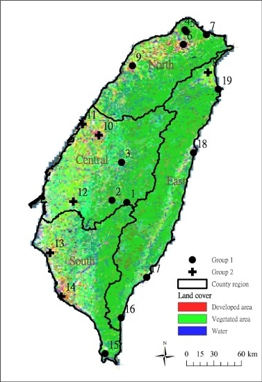
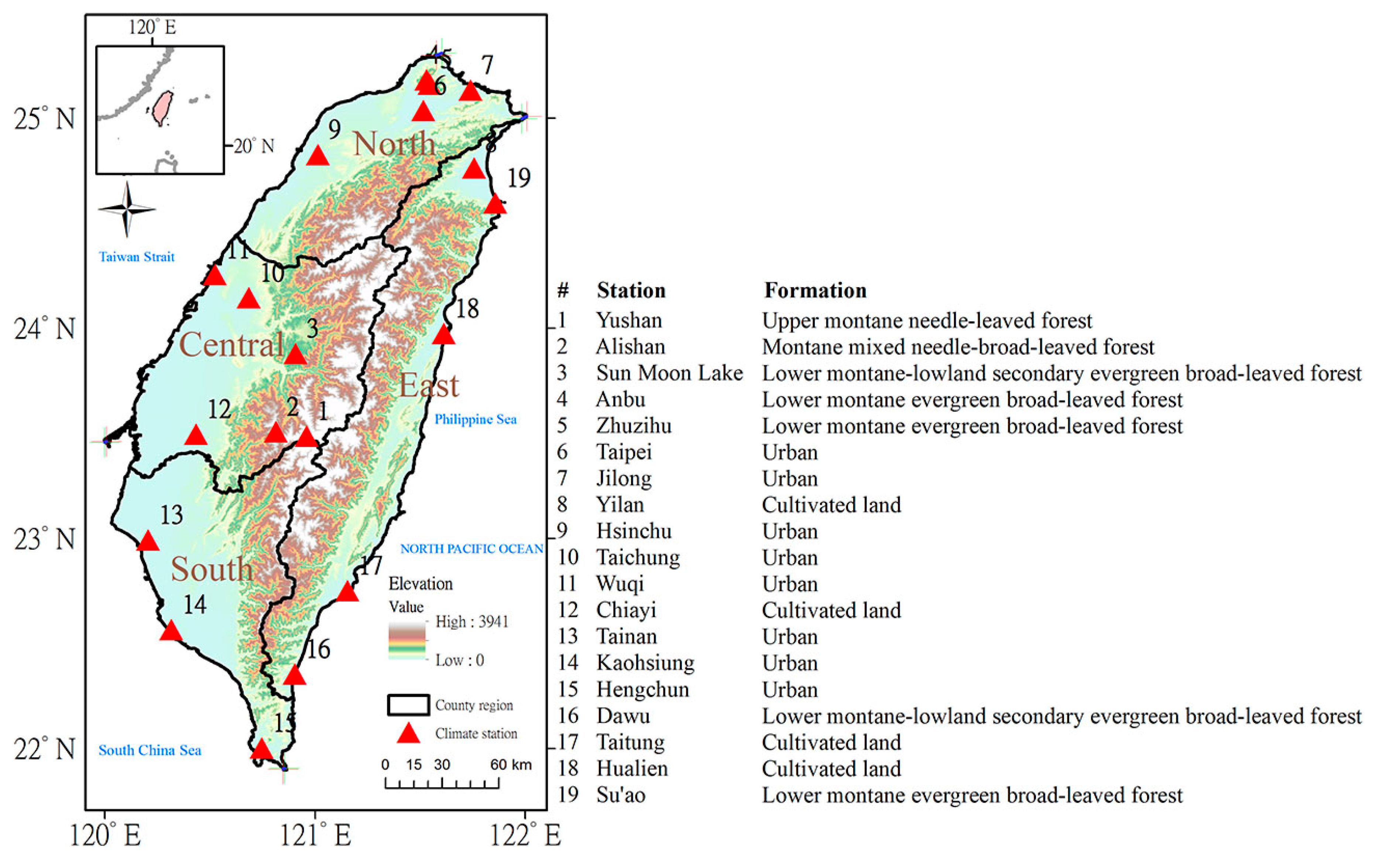
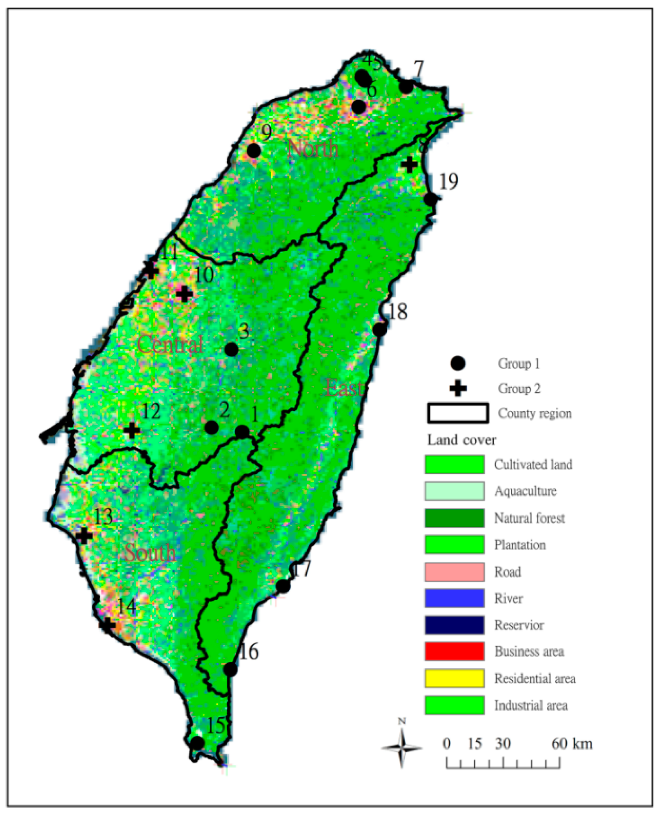
2.1. Study Area
2.2. Data Source
2.2.1. NDVI
2.2.2. Environmental Variables
3. Methods
3.1. Hierarchical Cluster Analysis (HCA)
3.2. Redundancy Analysis (RDA)
- The arrows point in the direction of maximum increase in the value of the variable across the diagram, and its length is proportional to this maximum rate of change.
- An approximate ordering of the value of one RV or EV across cases is obtained by projecting the case points perpendicular to the RV or EV arrow.
- A case point projecting onto the origin of the coordinate system (perpendicular to an RV or EV arrow) is predicted to have an average value of the corresponding variable. The cases projecting further from zero in the direction of the arrow are predicted to have above-average values, and the case points projecting in the opposite direction are predicted to have below-average values.
- The relative directions of arrows approximate the linear correlation coefficients among the variables. If an EV arrow points in a similar direction to an RV arrow, the values of that RV are predicted to be positively correlated with the EV values.
- The cosine of the angles between any two arrows indicates their respective relationship. If the arrows meet nearly at a right angle, these two variables are predicted to have a low (near to zero) correlation.
4. Results and Discussion
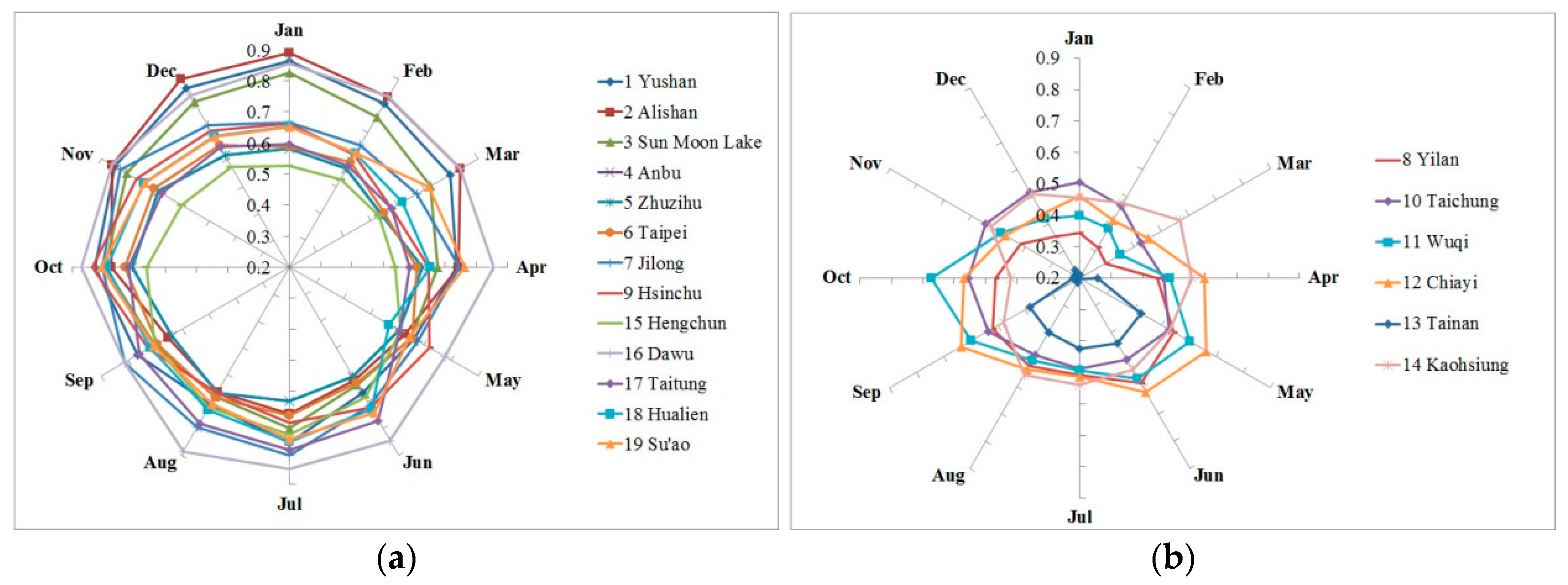
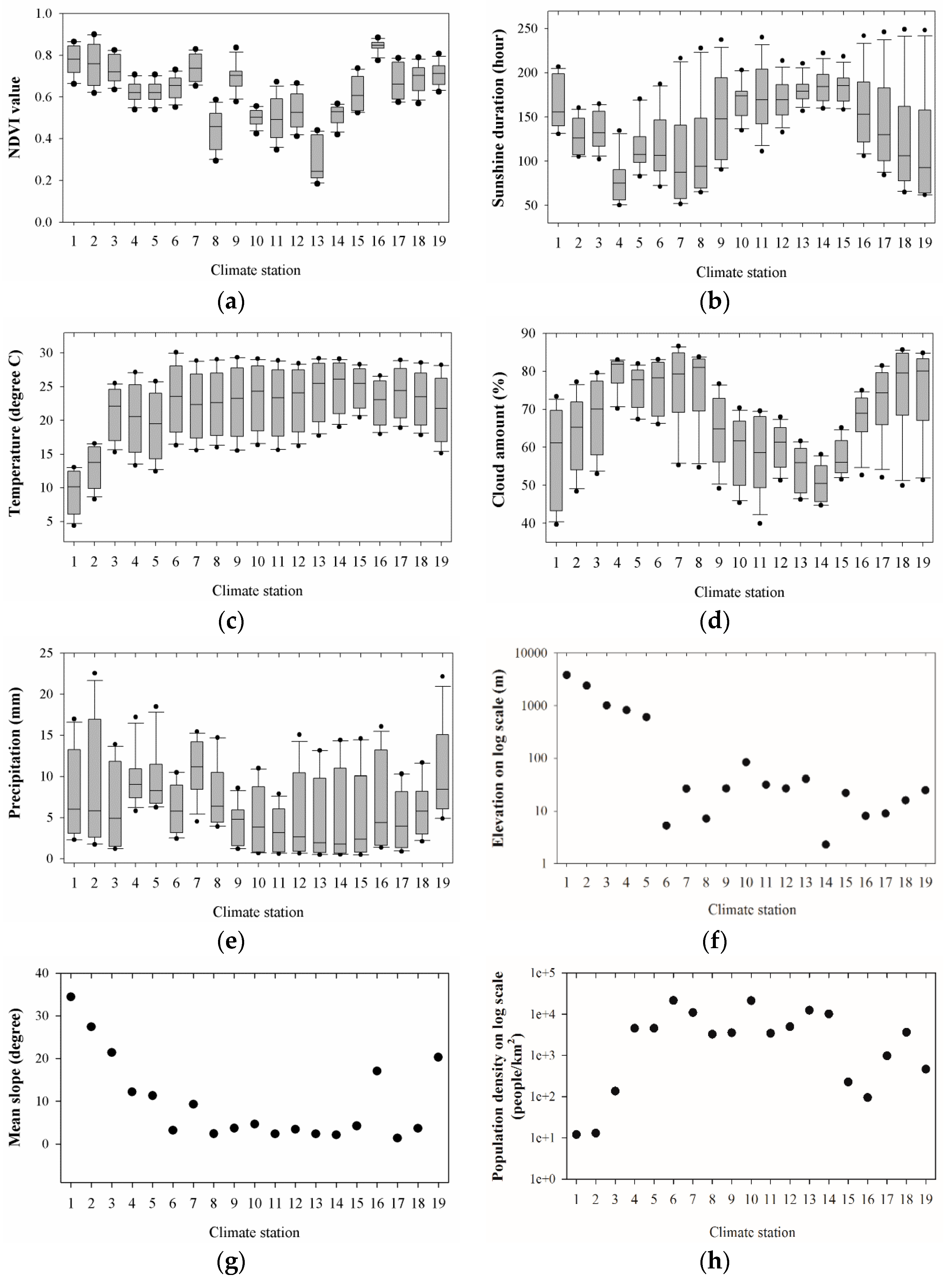
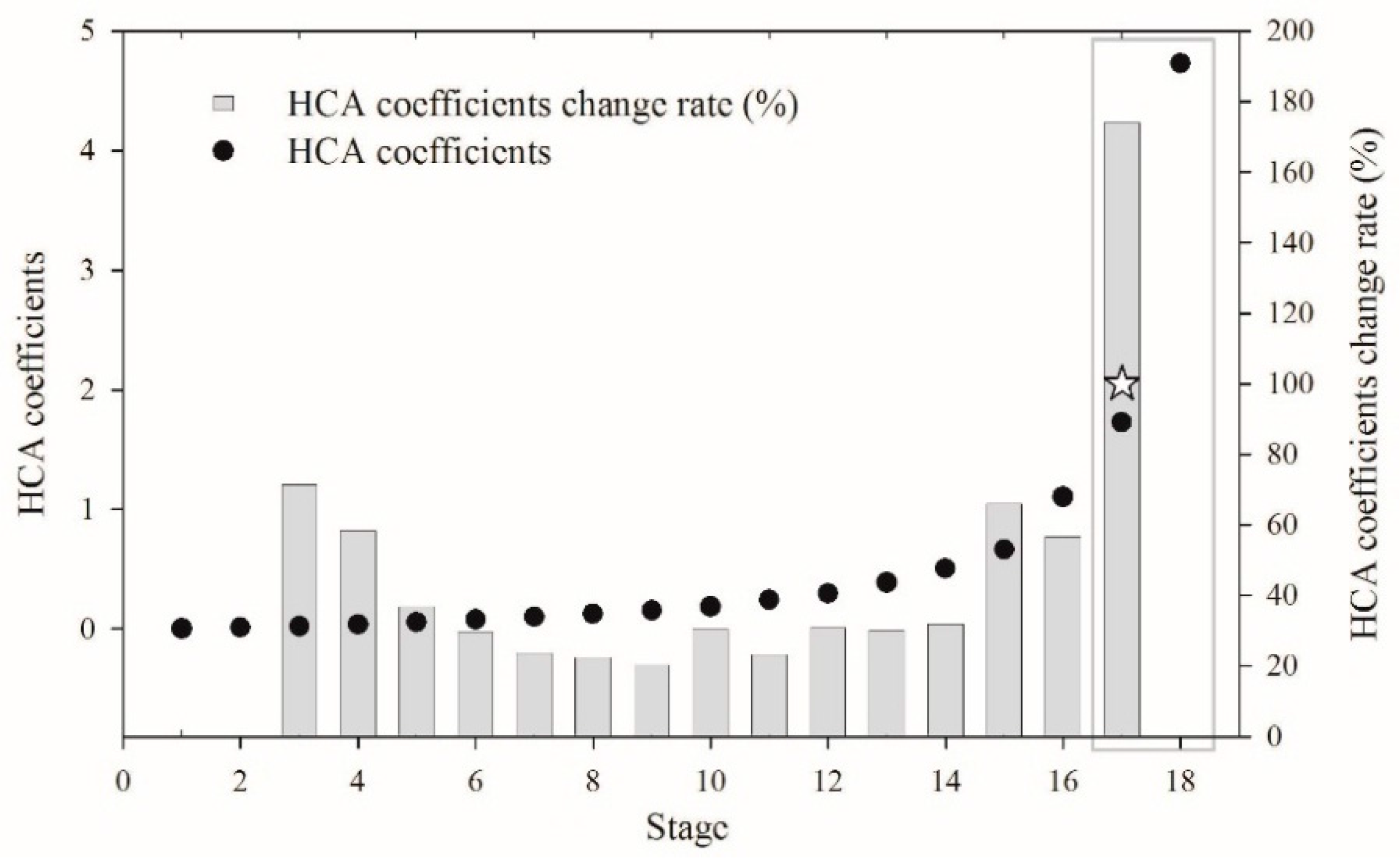
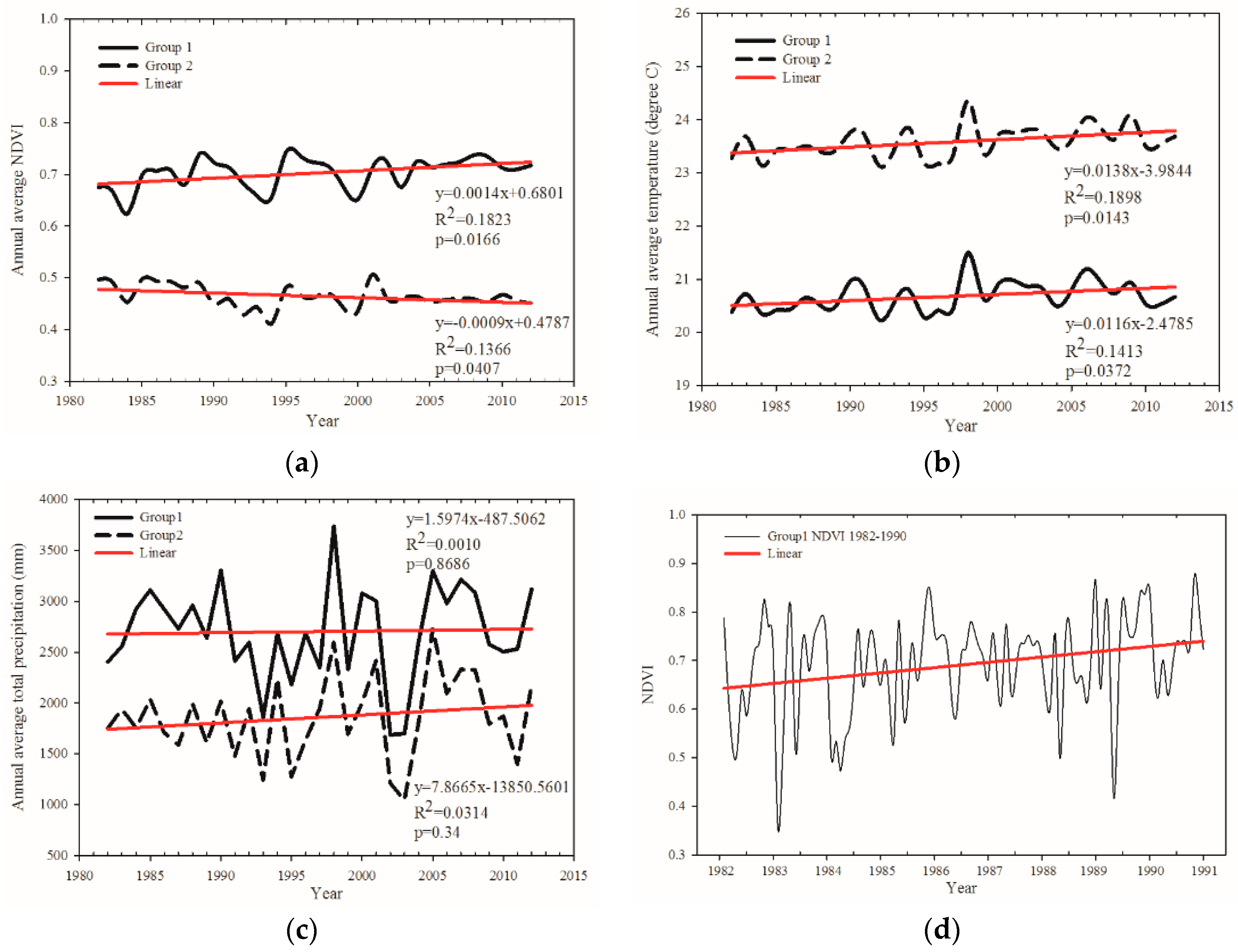
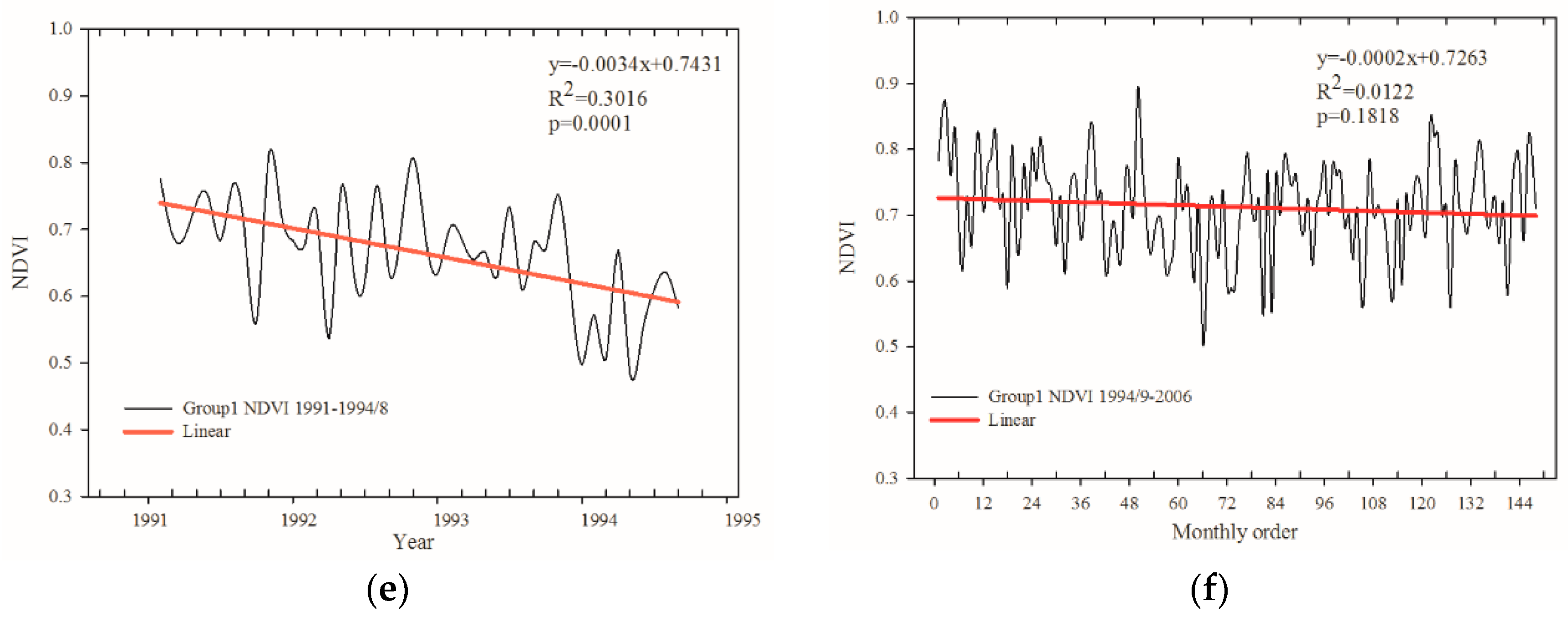
4.1. HCA
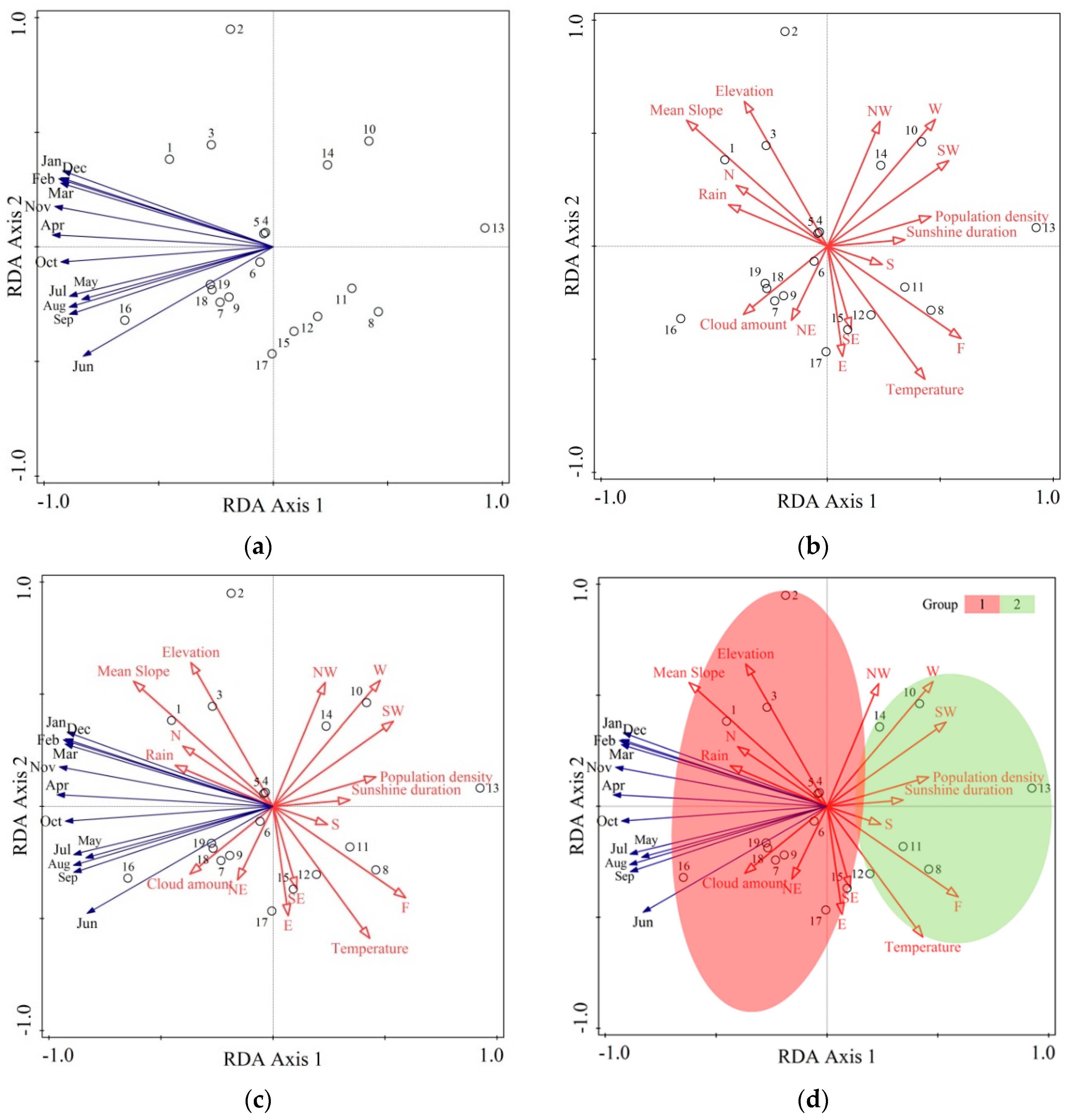
4.2. RDA
5. Conclusions
Acknowledgments
Author Contributions
Conflicts of Interests
References
- Qu, B.; Zhu, W.; Jia, S.; Lv, A. Spatio-temporal changes in vegetation activity and its driving factors during the growing season in China from 1982 to 2011. Remote Sens. 2015, 7, 13729–13752. [Google Scholar] [CrossRef]
- Cleland, E.E.; Chuine, I.; Menzel, A.; Mooney, H.A.; Schwartz, M.D. Shifting plant phenology in response to global change. Trends Ecol. Evol. 2007, 22, 357–365. [Google Scholar] [CrossRef] [PubMed]
- Chang, C.; Lin, T.; Wang, S.; Vadeboncoeur, M.A. Assessing growing season beginning and end dates and their relation to climate in taiwan using satellite data. Int. J. Remote Sens. 2011, 32, 5035–5058. [Google Scholar] [CrossRef]
- Pettorelli, N.; Vik, J.O.; Mysterud, A.; Gaillard, J.; Tucker, C.J.; Stenseth, N.C. Using the satellite-derived ndvi to assess ecological responses to environmental change. Trends Ecol. Evol. 2005, 20, 503–510. [Google Scholar] [CrossRef] [PubMed]
- Ransijn, J.; Kepfer-Rojas, S.; Verheyen, K.; Riis-Nielsen, T.; Schmidt, I.K. Hints for alternative stable states from long-term vegetation dynamics in an unmanaged heathland. J. Veg. Sci. 2015, 26, 254–266. [Google Scholar] [CrossRef]
- Yang, M.; Merry, C.J.; Sykes, R.M. Integration of water quality modeling, remote sensing, and GIS. J. Am. Water Resour. Assoc. 1999, 35, 253–263. [Google Scholar] [CrossRef]
- Yang, M.; Sykes, R.; Merry, C. Estimation of algal biological parameters using water quality modeling and SPOT satellite data. Ecol. Model. 2000, 125, 1–13. [Google Scholar] [CrossRef]
- Chang, C.; Wang, H.; Huang, C. Impacts of vegetation onset time on the net primary productivity in a mountainous island in Pacific Asia. Environ. Res. Lett. 2013, 8, 045030. [Google Scholar] [CrossRef]
- Hu, M.Q.; Mao, F.; Sun, H.; Hou, Y.Y. Study of Normalized difference vegetation index variation and its correlation with climate factors in the three-river-source region. Int. J. Appl. Earth Obs. 2011, 13, 24–33. [Google Scholar] [CrossRef]
- Mao, D.; Wang, Z.; Luo, L.; Ren, C. Integrating AVHRR and MODIS data to monitor NDVI changes and their relationships with climatic parameters in Northeast China. Int. J. Appl. Earth Obs. 2012, 18, 528–536. [Google Scholar] [CrossRef]
- He, B.; Chen, A.; Wang, H.; Wang, Q. Dynamic response of satellite-derived vegetation growth to climate change in the Three North Shelter Forest Region in China. Remote Sens. 2015, 7, 9998–10016. [Google Scholar] [CrossRef]
- Raynolds, M.; Magnússon, B.; Metúsalemsson, S.; Magnússon, S.H. Warming, sheep and volcanoes: Land cover changes in Iceland evident in satellite NDVI trends. Remote Sens. 2015, 7, 9492–9506. [Google Scholar] [CrossRef]
- Xu, G.; Zhang, H.; Chen, B.; Zhang, H.; Innes, J.L.; Wang, G.; Yan, J.; Zheng, Y.; Zhu, Z.; Myneni, R.B. Changes in vegetation growth dynamics and relations with climate over China’s landmass from 1982 to 2011. Remote Sens. 2014, 6, 3263–3283. [Google Scholar] [CrossRef]
- DeFries, R.; Townshend, J. NDVI-derived land cover classifications at a global scale. Int. J. Remote Sens. 1994, 15, 3567–3586. [Google Scholar] [CrossRef]
- Lin, J.; Yang, M.; Lin, B.; Lin, P. Risk assessment of debris flows in Songhe Stream, Taiwan. Eng. Geol. 2011, 123, 100–112. [Google Scholar] [CrossRef]
- Lunetta, R.S.; Knight, J.F.; Ediriwickrema, J.; Lyon, J.G.; Worthy, L.D. Land-cover change detection using multi-temporal MODIS NDVI data. Remote Sens. Environ. 2006, 105, 142–154. [Google Scholar] [CrossRef]
- Yang, M. A Genetic Algorithm (GA) based automated classifier for remote sensing imagery. Can. J. Remote Sens. 2007, 33, 203–213. [Google Scholar] [CrossRef]
- Yang, M.; Su, T.; Hsu, C.; Chang, K.; Wu, A. Mapping of the 26 December 2004 tsunami disaster by using FORMOSAT-2 Images. Int. J. Remote Sens. 2007, 28, 3071–3091. [Google Scholar] [CrossRef]
- Yang, M.; Lin, J.; Yao, C.; Chen, J.; Su, T.; Jan, C. Landslide-induced levee failure by high concentrated sediment flow—A case of Shan-an levee at Chenyulan River, Taiwan. Eng. Geol. 2011, 123, 91–99. [Google Scholar] [CrossRef]
- Peters, A.J.; Walter-Shea, E.A.; Ji, L.; Vina, A.; Hayes, M.; Svoboda, M.D. Drought monitoring with NDVI-based standardized vegetation index. Photogramm. Eng. Remote Sens. 2002, 68, 71–75. [Google Scholar]
- Vicente-Serrano, S.M.; Cabello, D.; Tomás-Burguera, M.; Martín-Hernández, N.; Beguería, S.; Azorin-Molina, C.; Kenawy, A.E. Drought variability and land degradation in semiarid regions: Assessment using remote sensing data and drought indices (1982–2011). Remote Sens. 2015, 7, 4391–4423. [Google Scholar] [CrossRef]
- Nemani, R.R.; Keeling, C.D.; Hashimoto, H.; Jolly, W.M.; Piper, S.C.; Tucker, C.J.; Myneni, R.B.; Running, S.W. Climate-driven increases in global terrestrial net primary production from 1982 to 1999. Science 2003, 300, 1560–1563. [Google Scholar] [CrossRef] [PubMed]
- Myneni, R.B.; Hall, F.G.; Sellers, P.J.; Marshak, A.L. The interpretation of spectral vegetation indexes. IEEE Geosci. Remote Sens. 1995, 33, 481–486. [Google Scholar] [CrossRef]
- Ichii, K.; Kawabata, A.; Yamaguchi, Y. Global correlation analysis for NDVI and climatic variables and NDVI trends: 1982–1990. Int. J. Remote Sens. 2002, 23, 3873–3878. [Google Scholar] [CrossRef]
- Krishnaswamy, J.; John, R.; Joseph, S. Consistent response of vegetation dynamics to recent climate change in tropical mountain regions. Glob. Chang. Biol. 2014, 20, 203–215. [Google Scholar] [CrossRef] [PubMed]
- Liu, Z.; Notaro, M.; Kutzbach, J.; Liu, N. Assessing global vegetation-climate feedbacks from observations. J. Clim. 2006, 19, 787–814. [Google Scholar] [CrossRef]
- Piao, S.; Mohammat, A.; Fang, J.; Cai, Q.; Feng, J. NDVI-Based increase in growth of temperate grasslands and its responses to climate changes in China. Glob. Environ. Chang. 2006, 16, 340–348. [Google Scholar] [CrossRef]
- Wang, J.; Rich, P.; Price, K. Temporal responses of NDVI to precipitation and temperature in the central great plains, USA. Int. J. Remote Sens. 2003, 24, 2345–2364. [Google Scholar] [CrossRef]
- Yang, M.; Yang, Y.; Hsu, S. Application of remotely sensed data to the assessment of terrain factors affecting the Tsao-Ling Landslide. Can. J. Remote Sens. 2004, 30, 593–603. [Google Scholar] [CrossRef]
- Zhu, L.; Southworth, J. Disentangling the Relationships between net primary production and precipitation in Southern Africa Savannas using satellite observations from 1982 to 2010. Remote Sens. 2013, 5, 3803–3825. [Google Scholar] [CrossRef]
- Tan, J.; Piao, S.; Chen, A.; Zeng, Z.; Ciais, P.; Janssens, I.A.; Mao, J.; Myneni, R.B.; Peng, S.; Peñuelas, J. Seasonally different response of photosynthetic activity to daytime and night-time warming in the Northern Hemisphere. Glob. Chang. Biol. 2015, 21, 377–387. [Google Scholar] [CrossRef] [PubMed]
- Fang, J.; Piao, S.; Field, C.B.; Pan, Y.; Guo, Q.; Zhou, L.; Peng, C.; Tao, S. Increasing net primary production in China from 1982 to 1999. Front. Ecol. Environ. 2003, 1, 293–297. [Google Scholar] [CrossRef]
- Mao, J.; Shi, X.; Thornton, P.E.; Piao, S.; Wang, X. Causes of spring vegetation growth trends in the northern mid–high latitudes from 1982 to 2004. Environ. Res. Lett. 2012, 7, 014010. [Google Scholar] [CrossRef]
- Myneni, R.B.; Keeling, C.; Tucker, C.; Asrar, G.; Nemani, R. Increased plant growth in the northern high latitudes from 1981 to 1991. Nature 1997, 386, 698–702. [Google Scholar] [CrossRef]
- Chen, B.; Xu, G.; Coops, N.C.; Ciais, P.; Innes, J.L.; Wang, G.; Myneni, R.B.; Wang, T.; Krzyzanowski, J.; Li, Q. Changes in vegetation photosynthetic activity trends across the Asia-Pacific region over the last three decades. Remote Sens. Environ. 2014, 144, 28–41. [Google Scholar] [CrossRef]
- Yu, F.; Price, K.P.; Ellis, J.; Shi, P. Response of seasonal vegetation development to climatic variations in Eastern Central Asia. Remote Sens. Environ. 2003, 87, 42–54. [Google Scholar] [CrossRef]
- Wang, H.; Liu, D.; Lin, H.; Montenegro, A.; Zhu, X. NDVI and vegetation phenology dynamics under the influence of sunshine duration on the Tibetan Plateau. Int. J. Climatol. 2015, 35, 687–698. [Google Scholar] [CrossRef]
- Stocker, T.F.; Qin, D.; Plattner, G.K.; Tignor, M.; Allen, S.K. Climate Change 2013: The Physical Science Basis; Cambridge University Press: Cambridge, UK, 2014. [Google Scholar]
- Lim, B.; Burton, I. Development programme United Nations. In Adaptation Policy Frameworks for Climate Change: Developing Strategies, Policies and Measures; Cambridge University Press: Cambridge, UK, 2005. [Google Scholar]
- Munang, R.; Thiaw, I.; Alverson, K.; Mumba, M.; Liu, J.; Rivington, M. Climate Change and ecosystem-based adaptation: A new pragmatic approach to buffering climate change impacts. Curr. Opin. Environ. Sustain. 2013, 5, 67–71. [Google Scholar] [CrossRef]
- Jump, A.S.; Huang, T.; Chou, C. Rapid altitudinal migration of mountain plants in Taiwan and its implications for high altitude biodiversity. Ecography 2012, 35, 204–210. [Google Scholar] [CrossRef]
- Myers, N.; Mittermeier, R.A.; Mittermeier, C.G.; da Fonseca, G.A.; Kent, J. Biodiversity hotspots for conservation priorities. Nature 2000, 403, 853–858. [Google Scholar] [CrossRef] [PubMed]
- National Development Council. Adaptation Strategy to Climate Change in Taiwan. Available online: http://www.ndc.gov.tw/en/cp.aspx?n=97B9027210DBD173 (accessed on 24 March 2016).
- Lin, W.; Lin, C.; Chou, W. Assessment of vegetation recovery and soil erosion at landslides caused by a catastrophic earthquake: A case study in central Taiwan. Ecol. Eng. 2006, 28, 79–89. [Google Scholar] [CrossRef]
- Lee, T.; Yeh, H. Applying remote sensing techniques to monitor shifting wetland vegetation: A case study of Danshui River Estuary mangrove communities, Taiwan. Ecol. Eng. 2009, 35, 487–496. [Google Scholar] [CrossRef]
- Chen, Y.; Li, X.; Xie, F. NDVI changes in China between 1989 and 1999 using change vector analysis based on time series data. J. Geogr. Sci. 2001, 11, 383–392. [Google Scholar]
- Wang, H.; Huang, C. Retrieving multi-scale climatic variations from high dimensional time-series MODIS green vegetation cover in a tropical/subtropical mountainous island. J. Mt. Sci. 2014, 11, 407–420. [Google Scholar]
- Hsu, H.; Chou, C.; Wu, Y.; Lu, M.; Chen, C.; Chen, Y. Climate Change in Taiwan: Scientific Report 2011; National Science Council: Taipei, Taiwan, 2011; p. 67. [Google Scholar]
- Lee, M.; Lin, T.; Vadeboncoeur, M.A.; Hwong, J. Remote sensing assessment of forest damage in relation to the 1996 strong typhoon Herb at Lienhuachi experimental forest, Taiwan. For. Ecol. Manag. 2008, 255, 3297–3306. [Google Scholar] [CrossRef]
- Chen, C.; Chen, Y. The rainfall characteristics of Taiwan. Mon. Weather Rev. 2003, 131, 1323–1341. [Google Scholar] [CrossRef]
- Yen, M.; Chen, T. Seasonal variation of the rainfall over Taiwan. Int. J. Climatol. 2000, 20, 803–809. [Google Scholar] [CrossRef]
- Kuo, Y.; Lee, M.; Lu, M. Association of Taiwan’s rainfall patterns with large-scale oceanic and atmospheric phenomena. Adv. Meteorol. 2016, 2016, 3102895. [Google Scholar] [CrossRef]
- Council of Agriculture, Executive Yuan, Natural Vegetation Community in Taiwan. Available online: http://data.gov.tw/node/9930 (accessed on 26 March 2016).
- Vermote, E.; Kaufman, Y. Absolute calibration of AVHRR visible and near-infrared channels using ocean and cloud views. Int. J. Remote Sens. 1995, 16, 2317–2340. [Google Scholar] [CrossRef]
- Pinzon, J.; Brown, M.E.; Tucker, C.J. EMD correction of orbital drift artifacts in satellite data stream. In Hilbert-Huang Transform and its Applications; Huang, N.E., Shen, S.S., Eds.; World Scientific Publishing Co. Pte. Ltd.: Singapore, 2005; pp. 167–186. [Google Scholar]
- Pinzon, J.E.; Tucker, C.J. A non-stationary 1981–2012 AVHRR NDVI3g time series. Remote Sens. 2014, 6, 6929–6960. [Google Scholar] [CrossRef]
- Bi, J.; Xu, L.; Samanta, A.; Zhu, Z.; Myneni, R. Divergent arctic-boreal vegetation changes between North America and Eurasia over the past 30 years. Remote Sens. 2013, 5, 2093–2112. [Google Scholar] [CrossRef]
- Watson, D.F. Contouring: A Guide to the Analysis and Display of Spatial Data; Pergamon Press: Oxford, UK, 1992. [Google Scholar]
- Yang, M.; Su, T. Segmenting ideal morphologies of sewer pipe defects on CCTV images for automated diagnosis. Expert Syst. Appl. 2009, 36, 3562–3573. [Google Scholar] [CrossRef]
- Su, T.; Yang, M.; Wu, T.; Lin, J. Morphological segmentation based on edge detection for sewer pipe defects on CCTV images. Expert Syst. Appl. 2011, 38, 13094–13114. [Google Scholar] [CrossRef]
- Gauch, H.G., Jr.; Whittaker, R.H. Hierarchical classification of community data. J. Ecol. 1981, 537–557. [Google Scholar] [CrossRef]
- Huang, W.; Chen, W.; Chuang, Y.; Lin, Y.; Chen, H. Biological toxicity of groundwater in a seashore area: Causal analysis and its spatial pollutant pattern. Chemosphere 2014, 100, 8–15. [Google Scholar] [CrossRef] [PubMed]
- Ward, J.H., Jr. Hierarchical grouping to optimize an objective function. J. Am. Stat. Assoc. 1963, 58, 236–244. [Google Scholar] [CrossRef]
- Punj, G.; Stewart, D.W. Cluster analysis in marketing research: Review and suggestions for application. J. Market. Res. 1983, 134–148. [Google Scholar] [CrossRef]
- Fraley, C.; Raftery, A.E. How many clusters? Which clustering method? Answers via model-based cluster analysis. Comput. J. 1998, 41, 578–588. [Google Scholar] [CrossRef]
- Yim, O.; Ramdeen, K.T. Hierarchical cluster analysis: Comparison of three linkage measures and application to psychological data. Quant. Methods Psychol. 2015, 11, 8–24. [Google Scholar]
- Rao, C.R. The use and interpretation of principal component analysis in applied research. Sankhya Ser. A 1964, 26, 329–358. [Google Scholar]
- Van den Wollenberg, A.L. Redundancy analysis an alternative for canonical correlation analysis. Psychometrika 1977, 42, 207–219. [Google Scholar] [CrossRef]
- Gittins, R. Canonical Analysis; Springer: Heidelberg, Germany, 1985. [Google Scholar]
- Legendre, P.; Legendre, L.F. Numerical Ecology; Elsevier: Amsterdam, The Netherlands, 2012. [Google Scholar]
- Buttigieg, P.L.; Ramette, A. A guide to statistical analysis in microbial ecology: A community-focused, living review of multivariate data analyses. FEMS Microbiol. Ecol. 2014, 90, 543–550. [Google Scholar] [CrossRef] [PubMed]
- Lepš, J.; Šmilauer, P. Multivariate Analysis of Ecological Data using CANOCO; Cambridge University Press: Cambridge, UK, 2003. [Google Scholar]
- Ter Braak, C.J.; Smilauer, P. CANOCO Reference Manual and CanoDraw for Windows User's Guide: Software for Canonical Community Ordination (Version 4.5); Biometris: Wageningen, The Netherlands, 2002. [Google Scholar]
- Huang, W.; Lin, Y.; Chen, W.; Chen, H.; Yu, R. Causal relationships among biological toxicity, geochemical conditions and derived DBPs in groundwater. J. Hazard. Mater. 2015, 283, 24–34. [Google Scholar] [CrossRef] [PubMed]
- Šmilauer, P.; Lepš, J. Multivariate Analysis of Ecological Data Using CANOCO 5; Cambridge University Press: Cambridge, UK, 2014. [Google Scholar]
- Pearson, K. Mathematical contributions to the theory of evolution. On a form of spurious correlation which may arise when indices are used in the measurement of organs. Proc. R. Soc. Lond. 1896, 60, 489–498. [Google Scholar] [CrossRef]
- Trenberth, K.E.; Shea, D.J. Relationships between precipitation and surface temperature. Geophys. Res. Lett. 2005, 32. [Google Scholar] [CrossRef]
- Yeh, C. An Exploring History of Taiwan; Tai-Yuan Publications: Taipei, Taiwan, 1995. [Google Scholar]
- Koh, C.; Lee, P.; Lin, R. Bird species richness patterns of Northern Taiwan: Primary productivity, human population density, and habitat heterogeneity. Divers. Distrib. 2006, 12, 546–554. [Google Scholar] [CrossRef]
- Chen, S.; Kuo, C.; Yu, P. Historical trends and variability of meteorological droughts in Taiwan/Tendances historiques et variabilité des sécheresses météorologiques à Taiwan. Hydrol. Sci. J. 2009, 54, 430–441. [Google Scholar] [CrossRef]
- Karnieli, A.; Agam, N.; Pinker, R.T.; Anderson, M.; Imhoff, M.L.; Gutman, G.G.; Panov, N.; Goldberg, A. Use of NDVI and land surface temperature for drought assessment: Merits and limitations. J. Clim. 2010, 23, 618–633. [Google Scholar] [CrossRef]
- Lai, Y.; Chou, M.; Lin, P. Parameterization of topographic effect on surface solar radiation. J. Geophys. Res. Atmos. 2010, 115. [Google Scholar] [CrossRef]
- Shryock, D.F.; Esque, T.C.; Chen, F.C. Topography and Climate are more important drivers of long-term, post-fire vegetation assembly than time-since-fire in the Sonoran Desert, US. J. Veg. Sci. 2015, 26, 1134–1147. [Google Scholar] [CrossRef]
- Field, C.B.; Van Aalst, M. Climate Change 2014: Impacts, Adaptation, and Vulnerability; IPCC: Geneva, Switzerland, 2014. [Google Scholar]
- Hsu, H.; Chen, C. Observed and projected climate change in Taiwan. Meteorol. Atmos. Phys. 2002, 79, 87–104. [Google Scholar] [CrossRef]
- Guan, B.T.; Hsu, H.; Wey, T.; Tsao, L. Modeling monthly mean temperatures for the mountain regions of Taiwan by generalized additive models. Agric. For. Meteorol. 2009, 149, 281–290. [Google Scholar] [CrossRef]
- Yu, H.; Luedeling, E.; Xu, J. Winter and spring warming result in delayed spring phenology on the Tibetan plateau. Proc. Natl. Acad. Sci. USA 2010, 107, 22151–22156. [Google Scholar] [CrossRef] [PubMed]
- Yu, P.; Yang, T.; Kuo, C. Evaluating long-term trends in annual and seasonal precipitation in Taiwan. Water Resour. Manag. 2006, 20, 1007–1023. [Google Scholar] [CrossRef]
- Hung, C.; Kao, P. Weakening of the winter monsoon and abrupt increase of winter rainfalls over Northern Taiwan and Southern China in the early 1980s. J. Clim. 2010, 23, 2357–2367. [Google Scholar] [CrossRef]
- Wu, C.; Yen, T.; Kuo, Y.; Wang, W. Rainfall simulation associated with typhoon herb (1996) near Taiwan. Part I: The topographic effect. Weather Forecast. 2002, 17, 1001–1015. [Google Scholar] [CrossRef]
- Yu, P.; Yang, T.; Wu, C. Impact of climate change on water resources in Southern Taiwan. J. Hydrol. 2002, 260, 161–175. [Google Scholar] [CrossRef]
- Sherwood, S.; Fu, Q. Climate change. A drier future? Science 2014, 343, 737–739. [Google Scholar] [CrossRef] [PubMed]
- Trenberth, K.E.; Dai, A.; van der Schrier, G.; Jones, P.D.; Barichivich, J.; Briffa, K.R.; Sheffield, J. Global warming and changes in drought. Nat. Clim. Chang. 2014, 4, 17–22. [Google Scholar] [CrossRef]
- Shiu, C.; Liu, S.C.; Chen, J. Diurnally asymmetric trends of temperature, humidity, and precipitation in Taiwan. J. Clim. 2009, 22, 5635–5649. [Google Scholar] [CrossRef]
- Tu, J.; Chou, C. Changes in precipitation frequency and intensity in the vicinity of Taiwan: Typhoon versus non-typhoon events. Environ. Res. Lett. 2013, 8, 014023. [Google Scholar] [CrossRef]
- Chu, P.; Chen, D.; Lin, P. Trends in precipitation extremes during the typhoon season in Taiwan over the last 60 Years. Atmos. Sci. Lett. 2014, 15, 37–43. [Google Scholar] [CrossRef]
- Chang, C. The potential impact of climate change on Taiwan’s agriculture. Am. J. Agric. Econ. 2002, 27, 51–64. [Google Scholar] [CrossRef]


| Temperature | Precipitation | Cloud Amount | Sunshine Duration | Elevation | Population Density | Mean Slope | |
|---|---|---|---|---|---|---|---|
| Temperature | 1 | ||||||
| Precipitation | −0.489 * | 1 | |||||
| Cloud amount | −0.003 | 0.620 ** | 1 | ||||
| Sunshine duration | 0.178 | −0.747 ** | −0.935 ** | 1 | |||
| Elevation | −0.964 ** | 0.343 | −0.149 | −0.037 | 1 | ||
| Population density | 0.352 | −0.188 | −0.056 | 0.036 | −0.331 | 1 | |
| Mean slope | −0.864 ** | 0.570 * | 0.049 | −0.188 | 0.840 ** | −0.454 | 1 |
| Variable | Group 1 | Group 2 |
|---|---|---|
| NDVI | 0.70 (0.06) | 0.46 (0.08) |
| Temperature (degree C) | 20.68 (4.31) | 23.59 (0.89) |
| Precipitation (mm) | 7.51 (2.23) | 5.16 (1.22) |
| Cloud amount (%) | 69.83 (7.05) | 59.81 (7.92) |
| Sunshine duration (hour) | 133.03 (26.76) | 165.60 (22.55) |
| Elevation (m) | 680.38 (1132.47) | 32.15 (26.78) |
| Population density (people/km2) | 1796.98 (1867.16) * | 9243.00 (6373.49) |
| Mean slope (degree) | 13.06 (10.03) | 2.90 (0.89) |
| Flat (%) | 4.55 (3.81) | 8.80 (3.84) |
| North (%) | 12.37 (3.14) | 8.74 (2.38) |
| Northeast (%) | 12.37 (3.14) | 10.72 (3.27) |
| East (%) | 10.93 (4.35) | 10.83 (3.43) |
| Southeast (%) | 11.35 (4.93) | 12.58 (3.34) |
| South (%) | 12.19 (3.75) | 14.04 (2.73) |
| Southwest (%) | 11.72 (3.56) | 13.95 (2.39) |
| West (%) | 11.84 (4.14) | 14.39 (3.33) |
| Northwest (%) | 12.68 (4.11) | 13.67 (2.59) |
| NDVI | Axis 1 | Axis 1 and 2 | Total |
|---|---|---|---|
| January | 84.37 | 95.39 | 97.06 |
| February | 87.75 | 96.60 | 97.16 |
| March | 86.10 | 93.86 | 98.36 |
| April | 93.05 | 93.33 | 99.48 |
| May | 70.01 | 75.27 | 97.76 |
| June | 68.86 | 91.68 | 96.65 |
| July | 79.79 | 84.39 | 93.07 |
| August | 79.46 | 86.39 | 92.78 |
| September | 79.54 | 88.33 | 92.39 |
| October | 85.97 | 86.41 | 97.28 |
| November | 90.97 | 94.08 | 96.79 |
| December | 85.89 | 94.99 | 95.74 |
| Average | 82.65 | 90.06 | 96.21 |
| Simple Term Effect | Conditional Term Effect | |
|---|---|---|
| Name of variable | Explains % | Explains % |
| Mean Slope | 34.4 *** | 34.4 *** |
| F | 30.2 *** | 1.3 |
| SW | 25.1 ** | 0.7 |
| W | 21.7 ** | 27.4 *** |
| Temperature | 18 * | 6.6 |
| Population density | 17.7 * | 1.4 |
| Rain | 16.3 * | 1.1 |
| Elevation | 14.2 | 0.4 |
| N | 14.1 | 1.6 |
| Cloud amount | 12.4 | 1.6 |
| Sunshine duration | 10.1 | 2.7 |
| NW | 7.2 | 1.1 |
| S | 5 | 2.7 |
| NE | 3.6 | 1 |
| E | 3.2 | 2.2 |
| SE | 2.6 | 10.1 ** |
© 2016 by the authors; licensee MDPI, Basel, Switzerland. This article is an open access article distributed under the terms and conditions of the Creative Commons by Attribution (CC-BY) license (http://creativecommons.org/licenses/by/4.0/).
Share and Cite
Tsai, H.P.; Lin, Y.-H.; Yang, M.-D. Exploring Long Term Spatial Vegetation Trends in Taiwan from AVHRR NDVI3g Dataset Using RDA and HCA Analyses. Remote Sens. 2016, 8, 290. https://doi.org/10.3390/rs8040290
Tsai HP, Lin Y-H, Yang M-D. Exploring Long Term Spatial Vegetation Trends in Taiwan from AVHRR NDVI3g Dataset Using RDA and HCA Analyses. Remote Sensing. 2016; 8(4):290. https://doi.org/10.3390/rs8040290
Chicago/Turabian StyleTsai, Hui Ping, Yu-Hao Lin, and Ming-Der Yang. 2016. "Exploring Long Term Spatial Vegetation Trends in Taiwan from AVHRR NDVI3g Dataset Using RDA and HCA Analyses" Remote Sensing 8, no. 4: 290. https://doi.org/10.3390/rs8040290