On the Role of Land Surface Temperature as Proxy of Soil Moisture Status for Drought Monitoring in Europe

Abstract

Remotely sensed Land Surface Temperature (LST) represents a valuable source of data for a simple modelling of the dynamic of soil moisture (SM) over large areas. In this paper we evaluated the capability of LST monthly anomalies, derived from the MOD11C3 standard product, to capture the SM dynamic as modelled over Europe by means of an ensemble of three land surface models. The direct use of LST as proxy of SM outperformed other LST-derived quantities, such as surface-to-air temperature gradient and day-night temperature variations, returning significant correlation values over the whole domain. LST performed better over Southern Europe compared to the Northern part of the domain, with the best results over areas characterized by water-limited conditions and moderate stress. Additionally, the analysis of the contingency matrix shows that the LST model is skillful in capturing extreme dry SM events, and it also has a good overall capability to correctly detect the dry events in 66% of the cases, with an average probability of false alarm of about 30%. Overall, the use of LST anomalies seems a promising starting point for a reliable modelling of the SM dynamic with a minimum amount of information. Even if the adopted approach is simple, the results are encouraging for a practical use of LST in an operational drought monitoring system over the study area.

1. Introduction

Drought is a relatively common weather-related natural disaster, defined as a phenomenon that follows a precipitation shortage compared to the climatology of that area. It can manifest at different spatiotemporal scales depending on the degree of propagation of this shortage within the hydrological cycle; as a consequence, it may have impacts on a range of socio-economic compartments. Of particular interest for environmental studies are the so-called ecosystem/agricultural droughts, which are defined as a reduction in vegetation water availability that negatively affects ecosystem productivity [1]. Such droughts can be characterized by a rapid onset and, depending on the phenological stage, may have significant impacts in agricultural areas (see “flash drought” in [2]). A common way to quantify this reduction is through the monitoring of some vegetation-related hydrological quantities, such as the difference between actual and potential evapotranspiration or the soil water deficit. Operational monitoring systems of ecosystem drought are commonly based on data aggregated at a monthly scale [3,4], even if longer aggregation periods (3, 6, or 12 months) are also used, mainly for meteorological drought analyses. Additionally, due to the spatial nature of the ecosystem drought phenomenon, the use of already spatially distributed data for its monitoring is advisable.

Satellite Thermal Infra-Red (TIR) data are an invaluable source to obtain spatially distributed information on the Land Surface Temperature (LST), with increasing availability and reliability thanks to the growing number of launched sensors [5] and improvements in processing algorithms [6]. LST assumes a central role as control variable in several environmental processes, including the hydrology and carbon cycles, as well as in the land surface energy budget [7]. Indeed, LST is key in connecting hydrology and energy balance at the land surface by means of its function in both evaporation and transpiration processes. During dry conditions, plants tend to close their stomata to reduce root-zone water loss through transpiration, and this closure results in a rise in leaf temperature; similarly, once the shallow soil (first few centimeters) dries out, the evaporation process stops and soil surface temperature rapidly increases. Overall, a clear inverse relationship between LST and the combined evapotranspiration (ET) process is observed in water-limited environments [8].

However, other factors, such as vegetation and snow coverage, also play a role in controlling LST; generally, a negative relationship has been observed between LST and vegetation coverage derived from remotely sensed indices (e.g., normalized difference vegetation index—NDVI) [9,10], especially during summer months [11]. The presence of a significant amount of snow coverage complicates the interpretation of the relationship between vegetation indices and LST, mainly due to the influence of snow on the land surface thermal regime [12].

LST has been used to characterize ecosystem drought using a wide range of methodologies, as summarized in [13]. On one hand, LST and NDVI–derived indices have been coupled for the estimation of combined indicators [14], or their strong inverse relationship has been used in the context of simple semi-empirical approaches to derive ET-related quantities; this is the case in the well-known trapezoid and triangle methods [15,16], in which the feature space LST-NDVI is analyzed to derive various plant water stress indices. On the other hand, the relationship between LST and NDVI suggests that the variations in vegetation amount are somehow accounted for in the LST data itself. This latter consideration is supported by the theoretical shape of the LST-NDVI feature space adopted in the above-mentioned methods, which suggests: (i) a larger variability in wet to dry bare soil LST compared to fully vegetated conditions; and (ii) a decreasing trend in the average LST with NDVI.

Another use of LST to quantify the effects of water deficit on ecosystems is within the context of the so-called residual surface energy balance approaches. These methods estimate the actual ET fluxes as residual of a simplified energy budget by exploiting the direct connection between the land surface-air temperature gradient and the sensible heat flux [17]. In this framework, LST is used as proxy of the aerodynamic temperature, and the surface-to-air temperature difference (ΔT) is proven to be inversely related to ET, as well as directly proportional to the soil water deficit that controls the ET process.

The idea of using ΔT rather than LST as proxy of the soil water deficit was also investigated in the context of the triangular/trapezoid methods, where the use of the feature space LST-NDVI, rather than ΔT-NDVI, is seen as a simplification forced by the common lack of auxiliary meteorological data [18]. To partially overcome this drawback, some authors suggested the use of the night-day temperature gradient as proxy of ΔT (e.g., [19,20]). A clear advantage of this solution is the full exploitation of the common availability of dual-time acquisitions of LST by the same sensor, limiting inconsistencies in the adopted LST datasets.

This brief overview points out a general agreement on the great informative content of LST as proxy of soil moisture deficit, even if it also clearly highlights the absence of a unanimous consensus on the best LST-related quantity to be used for proper quantification of the occurrence of significant variations in soil moisture deficit status. The ambiguity is even more marked if large-scale estimations (i.e., continental, global) are desirable, since most of the simplified approaches rely on hypotheses that do not hold on such large areas (e.g., spatial-constant meteorological forcing), whereas more complex physically-based energy balance approaches may require a large amount of difficult-to-retrieve auxiliary information (see [21]). The overview also highlights a main focus of the literature on single-day estimates, with few efforts made to take advantage of the growing temporal extension of the datasets collected by remote sensors.

In this context, it may be of interest to evaluate the actual value of remotely-sensed LST in capturing the spatiotemporal dynamic of soil moisture, given the limited need of further auxiliary information and the current availability of LST products in a near-real-time fashion. From this premise, the goal of this study is to evaluate different sets of LST-related quantities against modelled soil moisture maps used to derive information on the occurrence of past drought events. The reference dataset is constituted by an ensemble of three land surface models (LISFOOD, CLM and TESSEL), which demonstrated a good capability to capture variations in actually observed soil moisture and evapotranspiration records over Europe [22]. The use of modelled soil moisture as benchmark, rather than actual observations, allows overcoming the limitation related to the current lack of a dense network of soil moisture or ET measurements with adequate long-term records. The focus on Continental Europe is advised by a potential use of the study outcomes in the European Drought Observatory (EDO, http://edo.jrc.ec.europa.eu) for an operational near-real time monitoring of ecosystem drought.

2. Materials and Methods

2.1. Theoretical Background

The use of soil moisture (SM) data in drought monitoring applications is supported by the assumption that its deviation from the normal climatology is a good measure of the dryness of the soil, a key feature of a drought event, defined as a period of unusually low vegetation water availability. Since both SM and LST are characterized by a marked seasonality, the latter must be removed from the actual data in order to be able to evaluate the capability of one variable to capture the “non-obvious” dynamic of the other. The use of standardization procedures is a commonly accepted concept in time-series analyses, with standardized anomalies being more suitable for a proper statistical investigation of the correlation between two random variables obtained as the departure from the climatologies of the two data series [23]. Additionally, anomalies are more suited to respond to the question “is the soil currently drier or wetter than usual in the given location and time of the year?” than the direct use of other normalized indicators, such as in [14,24].

In this study, the standardization is performed on monthly data for all the analyzed quantities through the computation of z-scores, as:

$$z_{x,i,k}=\frac{x_{i,k}-{\mathsf{\mu }}_{x,i}}{{\mathsf{\sigma }}_{x,i}}$$

(1)

where x_i,k is the monthly average variable for the i-th month at the k-th year, μ_x,i and σ_x,i are the long-term average and standard deviation of the variable x for the i-th month, respectively. The monthly value of μ and σ are computed on a dataset collected in a reference period called baseline, which should be long enough to return a stable reference for the standardization (i.e., 15 to 30 years).

As previously discussed in the introduction, some authors have observed a positive relationship (and sometimes no correlation) between NDVI and LST during winter time, mainly explained by the influence of the extension of snow coverage on the surface thermal regime [11]. This may cause regional differences in the sign of the relationship LST-SM. Since ecosystem drought studies usually focus on the warm season only, we decided to concentrate the analysis only on the warm months over the European domain. This approach is quite common also in surface energy balance studies, since ET fluxes are predominant during the hottest period of the year (due to the high radiation forcing).

Warm season months were selected starting from monthly-mean daytime air temperature records collected over eleven cities spread across the European domain. The monthly data were normalized by means of the year average and standard deviation, and the warm season was defined as the period in which the normalized values were greater than 0 (i.e., it includes all months warmer than the year average).

As depicted in Figure 1, there is a general agreement in all the sites on identifying the period between May and October as the warm season (according to the previously reported definition). Only two sites (Minsk and Budapest) have positive normalized temperature also for April, but overall it is possible to state that the domain can be uniformly divided into two 6-month periods: (1) a cold season from November to April; and (2) a warm season between May and October. It is worth pointing out that the warm season coincides with the common dry season for the Mediterranean countries.

Figure 1. Normalized monthly-mean daytime air temperature (T_a) as recorded in eleven main cities spread across Europe. The grey-filled area highlights the warm season, as the months with temperature greater than the average (deseasonalized value > 0).

Figure 1. Normalized monthly-mean daytime air temperature (T_a) as recorded in eleven main cities spread across Europe. The grey-filled area highlights the warm season, as the months with temperature greater than the average (deseasonalized value > 0).

LST data can be directly used in Equation (1) to derive anomalies (x = LST) and the same can be made for the benchmark soil moisture dataset (x = SM); however, as briefly described in the introduction, other LST-related quantities are commonly used as proxy of the soil moisture status. Here, we analyzed three main variables: the air-to-surface temperature gradient, x = ΔT, computed as the difference between LST and air temperature; the day-night LST variation, x = ΔLST, computed as the difference between daytime and nighttime remote sensing LST acquisitions; and the air temperature itself, x = T_a. The inclusion of the first two variables is suggested by their use in several energy balance, triangle/trapezoidal methods, as well as thermal inertia applications, whereas the latter is used as a reference value on the informative content of the simple weather variation in atmospheric temperature.

Due to the expected inverse relationship between SM and the four investigated quantities, the sign of z_SM is reversed in order to simplify the straightforward comparison of the different standardized quantities. For the sake of simplicity, from now on, the SM anomalies are named “observed”, whereas the LST-derived anomalies are named “modelled”.

The overall capability of each of these four LST-related quantities to capture the fluctuations of SM is quantified in terms of the Pearson product-moment correlation coefficient (R), computed on the full sample constituted by N = n × 6 monthly values (with n number of years). The significance of the obtained correlation values is quantified according to critical values computed for p = 0.05 (R_0.05), as in the Student’s t-distribution test.

Furthermore, a more specific analysis focused on the dry extremes (z_SM > 1), only it was performed starting from the construction of the contingency table [25]. Assuming the correct detection of the occurrence of z_SM > 1 (namely “events”) as the target goal, each pair of monthly anomalies (observed + modelled) can be classified as: hit, an observed event is correctly modelled; false alarm, a modelled event does not correspond to an observed one; miss, an observed event is not correctly modelled; correct reject, the absence of an observed event is correctly modelled.

For each model, it is possible to compute the total number of months with hits, false alarms, misses, and correct rejects, namely a, b, c, and d, respectively (a + b + c + d = N). These four quantities allow the definition of the Probability of Detection (POD) as well as the Probability of False Detection (POFD) indices, as:

$$\text{POD}=\frac{a}{a+c}$$

(2)

$$\text{POFD}=\frac{b}{b+d}$$

(3)

which quantify the ability of modelled values to capture the observed events and the fraction of the observed non-events that are wrongly identified as events by the model, respectively. Both indices range between 0 and 1, where 1 is the best score for POD (all the observed events are also modelled), whereas 0 is the best score for POFD (no false alarms).

It is clear that both POD and POFD only partially capture the behavior of the model, and the related best score does not correspond automatically to a perfect model. In order to quantify how good a model is overall, skill scores are introduced by comparing the performance of the model with a reference case, usually constituted by a random modelling of the event.

On the basis of these premises, the Heidke Skill Score (HSS) is introduced [26]:

$$\text{HSS}=\frac{ad-bc}{\left[\left(a+c\right)\left(c+d\right)+\left(a+b\right)\left(b+d\right)\right]/2}$$

(4)

where negative values correspond to models less skillful than the reference case (random) and a value of 1 represents a perfect model. HSS values above 0 represent the fraction of non-randomly predictable events that are correctly captured by the model.

2.2. MODIS LST Dataset

The main focus of the analysis is the use of remotely-sensed LST maps available at a monthly scale over a long time-frame. The dataset collected by the Moderate-Resolution Imaging Spectroradiometer (MODIS) sensor on board of the Terra satellite (http://terra.nasa.gov/about/terra-instruments/modis) fulfills these conditions. In particular, the MOD11C3 Monthly CMG (Climate Modelling Grid) LST product is used in this study, which is constituted by monthly composited and averaged temperature and emissivity maps at a spatial resolution of 0.05 degrees over a regular latitude/longitude grid for the period 2001–2013 (n = 13).

The monthly values in the product are obtained as a simple average of the MOD11C1 product maps in monthly calendar days, limited to the data collected under clear-sky conditions. The product includes both day and night maps, as well as the corresponding averaged observation times and viewing zenith angles. The daily values in the MOD11C1 product are derived by re-projection and averaging the values in the daily MOD11B1, which is available at 5 km equal-area grids in the standard MODIS sinusoidal projection. In order to include only clear-sky data into the MOD11C1 product, the cloud-contaminated daytime and nighttime LST values are preliminarily removed by means of a double-screen scheme [27]. This procedure makes a first screen based on the difference between the LST values retrieved with two methods: the day/night algorithm [28] and the generalized split-window algorithm [29]. Successively, the histogram of the difference between daytime and nighttime LSTs is used to remove the cells likely contaminated by clouds.

Daytime monthly images are directly used as inputs in Equation (1) for the LST dataset, whereas nighttime images are used in addition to daytime ones to derive the ΔLST dataset. The air temperature maps required for the ΔT dataset, as well as for the T_a dataset itself, were obtained from the daily meteorological records available in the EU-FLOOD-GIS database [30]. This dataset includes daily maps of minimum, maximum, and mean air temperature, which were used to obtain an estimate of the air temperature at the averaged LST observation time following the sinusoidal model [31]. Afterwards, daily data were combined into monthly data as simple averages, analogously to the procedure adopted for the LST product.

In order to spatially co-register the LST datasets (provided on a 0.05 degree regular latitude/longitude grid) over the T_a and SM maps (described in the next section), the monthly LST and ΔLST maps were re-projected into the ETRS89 Lambert Azimuthal Equal Area Coordinate System (ETRS-LAEA) and resampled at 5 km resolution using the nearest neighborhood method (in order to preserve the original data). Finally, the ΔT maps were computed directly on this map projection system for all months, including both warm and cold seasons.

2.3. Soil Moisture Benchmark Dataset

The SM benchmark dataset is made up of the ensemble of three land-surface model simulations, as fully described in [22]. In brief, the outputs of the LISFLOOD distributed hydrological rainfall-runoff model [32], the Community Land Model (CLM) [33], and the Tiled ECMWF (European Centre for Medium-range Weather Forecasts) Scheme of Surface Exchanges over Land (TESSEL) [34] were combined by means of a simple multi-model equal-weight ensemble [35]. The ensemble procedure was applied to the z-score values computed for each dataset separately, in order to minimize the problems related to the likely biases among the three time series. The ensemble dataset is constituted by monthly anomalies between 2001 and 2013 at 5 km resolution in the ETRS-LAEA system.

More details on the characteristics of the run of each model (i.e., parameterization, meteorological forcing, resolutions), as well as a detailed validation of the ensemble product through in situ measurements of both soil moisture and evapotranspiration is reported in [22]. In summary, the validation against in situ measurements suggested that the use of an ensemble of models rather than a single model is able to improve both the overall correlation with the observations and the skill of the model, while also showing the ability to reduce the number of dry event false alarms. In addition, the use of models based on local meteorological forcing data rather than global datasets suggests an improved confidence in the quality of the results.

Additionally, for an independent check of the tested LST-based indicators, the remotely sensed active and passive microwave merged product (Climate Change Initiative Soil Moisture, CCI-SM) developed by [36] has been used. This product is freely available as daily global maps at 0.25° spatial resolution, representing the skin soil moisture (0.5 to 2 cm) obtained as a combination of several microwave sensors (SSM/I, , AMSR, ASCAT, among others). Data for the period 2001–2013 were obtained from the product version v02.1.

3. Results and Discussion

The first analysis aims to evaluate which of the four LST-derived anomaly datasets better captures the dynamic of z_SM over the whole period constituted by the warm seasons (May to October) of the years 2001–2013 (N = 78). The maps in Figure 2 depict the spatial distribution of the R values between the anomalies of SM and: (a) LST; (b) ΔT; (c) ΔLST; and (d) T_a. This index highlights the existence of a direct linear relationship between the two random quantities; it is worth reminding that the sign of the z_SM values was changed due to the expected inverse relationship with the LST-derived quantities.

The spatial distributions of the values in Figure 2 show some similarities in the patterns of the four maps, with higher values in South-East Europe and lower values in the Northern part of the domain. Overall, it is possible to notice a better performance of LST compared to both ΔT and ΔLST, and a clear decay in the correlation in the case of T_a. This last result is rather expected, highlighting an evident added value to using LST over the simple meteorological air temperature. It is worth pointing out that this ranking remains the same even if the analysis is performed on the whole year (not shown), but with a notable reduction in the R values (as fully discussed successively).

A deeper analysis of the maps in Figure 2 highlights that the discrepancies between LST and ΔT/ΔLST are generally more marked over mountainous areas (i.e., Alps, Carpathians, Pyrenees), as well as over the Scandinavian Peninsula. Those areas are usually characterized by a significant amount of snow coverage during winter months, which may also cause the presence of permanent snow and snow melting phenomena during part of the warm season, which in turn may affect the thermal regime. Additionally, the energy budgets of steep areas, like mountains, are influenced by local exposition and solar incident angle phenomena that may not be properly accounted for in low spatial resolution models.

Figure 2. Spatial distribution of the Pearson correlation coefficient (R) between soil moisture anomalies and (a) land surface temperature (LST) anomalies; (b) air-to-surface temperature gradient anomalies; (c) LST day-night temperature difference anomalies; (d) air temperature anomalies. R values are computed on monthly data during the warm seasons (May–October) of 2001–2013. Values in yellow and red are not significant at p = 0.05.

Figure 2. Spatial distribution of the Pearson correlation coefficient (R) between soil moisture anomalies and (a) land surface temperature (LST) anomalies; (b) air-to-surface temperature gradient anomalies; (c) LST day-night temperature difference anomalies; (d) air temperature anomalies. R values are computed on monthly data during the warm seasons (May–October) of 2001–2013. Values in yellow and red are not significant at p = 0.05.

The overall better performance of LST compared to the other cases is also highlighted by the data reported in Table 1, where the average R and its standard deviation are reported for the whole domain (excluding bodies of water), as well as the fraction of the domain (expressed as percentage) with an R value greater than the one corresponding to a significance level of p = 0.05.

The results for the LST are characterized by the highest spatial-average value (0.48), combined with the lowest variability (0.17) and the highest fraction of the domain with significant values at p = 0.05 (almost 92%). As already highlighted by the maps in Figure 2b,c, the data in Table 1 confirm that ΔT and ΔLST seem to perform quite closely, which is also confirmed by the fraction of the domain with significant values (about 83% for both). The only variable that performs relatively poorly is T_a, which, however, has some informative content over South-East Europe. The comparison against the CCI-SM product shows similar findings, with LST slightly outperforming the other methods and spatial patterns similar to the ones reported in Figure 2 (not shown). The lower values observed against CCI-SM compared to the ensemble SM can be related to the low spatial resolution of the former (0.25°), as well as the reduced vertical resolution and the presence of several missing days in the dataset.

Table 1. Average statistics of the correlation analysis performed between anomalies of soil moisture (both ensemble and CCI-SM) and different temperature-related quantities.

Case		R avg.	R std. dev.	% Domain R > R0.05
LST	vs. Ensemble	0.48	0.17	91.8
ΔT		0.39	0.20	83.9
ΔLST		0.43	0.21	82.6
Ta		0.30	0.17	64.1
LST	vs. CCI-SM	0.31	0.25	68.2
ΔT		0.29	0.24	61.3
ΔLST		0.28	0.21	61.9
Ta		0.05	0.27	30.1

Table 1. Average statistics of the correlation analysis performed between anomalies of soil moisture (both ensemble and CCI-SM) and different temperature-related quantities.

Case		R avg.	R std. dev.	% Domain R > R0.05
LST	vs. Ensemble	0.48	0.17	91.8
ΔT		0.39	0.20	83.9
ΔLST		0.43	0.21	82.6
Ta		0.30	0.17	64.1
LST	vs. CCI-SM	0.31	0.25	68.2
ΔT		0.29	0.24	61.3
ΔLST		0.28	0.21	61.9
Ta		0.05	0.27	30.1

The observed decrease in R values when gradient quantities are used rather than the simple LST may be explained by the informative content associated with both nighttime LST and T_a. Indeed, even if ΔT is conceptually better connected with the magnitude of evaporative and sensible heat fluxes, a different analysis strategy is required when anomalies are investigated rather than the actual magnitude of the fluxes. The map in Figure 2d shows that T_a itself also has the capability to detect fluctuations in SM in some areas; however, the use of ΔT rather than LST has the effect of removing part of the information content in LST rather than improving the prediction capability (see Figure 2b vs. Figure 2a). Similar considerations can be made for ΔLST, since nighttime temperature is only used as a proxy of air temperature in triangular/trapezoid methods, whereas thermal inertia is commonly reliable only for bare soil or sparsely vegetated surfaces. Moreover, the similarities in the behavior of ΔT and ΔLST suggest a limited negative impact of the use of ground-observed T_a data in conjunction with remotely-sensed LST, hence the possible inconsistency between the two datasets due to the well-known issues on remote-sensing data absolute calibration and correction [37], as well as the likely inconsistency that arose during the monthly aggregation procedure.

Overall, it is a clear outcome of this comparison that LST performs better than the other indices both on average and over the spatial domain. The spatial distribution of the R values in Figure 2 highlights that the values for LST are consistently higher than the others for the whole study area, and the 10% of the domain with non-significant correlation values is substantially limited to the high mountain part of the Scandinavian Peninsula and the Ukrainian portion of the Carpathian Mountains. As a consequence, the use of LST as proxy of SM dynamic seems the best choice among the tested ones, and successive analyses will be focused on further investigating the use of z_LST as predictor of z_SM.

In order to better exemplify the actual value of LST as SM proxy and its capability to capture specific periods, a visual representation of four time-series of anomalies is depicted in Figure 3, showing the results for a range of R values including a high-R site in Romania (R = 0.8), an average-R site in Spain (R = 0.5), a barely-significant site in France (R = 0.3) and a non-significant site in Sweden (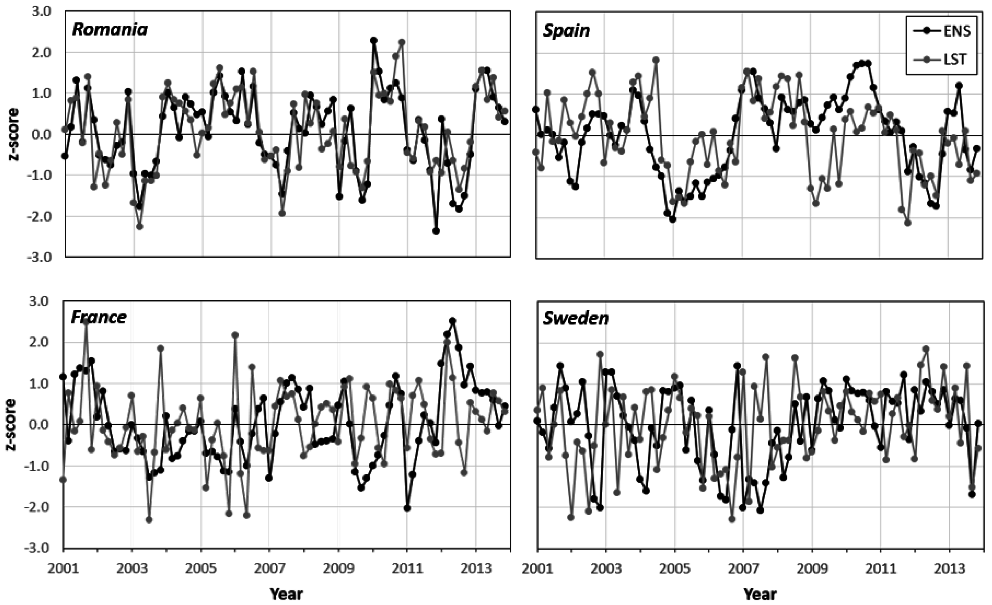R = 0.15). For all the sites only the data of the warm seasons are reported in the plots.

Figure 3. Examples of time-series of ensemble soil moisture (ENS) and land surface temperature (LST) monthly anomalies. Only the data during the warm seasons (May–October) are reported in the plots.

Figure 3. Examples of time-series of ensemble soil moisture (ENS) and land surface temperature (LST) monthly anomalies. Only the data during the warm seasons (May–October) are reported in the plots.

The times-series of anomalies in the upper line of Figure 3 (Romania and Spain) highlight the good agreement between the LST and the SM anomaly datasets, with only few misinterpreted events in Spain that justify the lower R value compared to the Romania site. It is also interesting to highlight that the general dynamic of SM anomalies is also captured by LST in the two sites characterized by a lower correlation (e.g., period of positive values in Sweden after 2009), even if some sparse substantial discrepancies can be clearly observed over these sites. Overall, the presence of persistent periods of positive/negative SM anomalies in the four cases is captured by LST in most of the cases, even when anomaly values for LST and SM for a specific month disagree.

A further analysis of the map in Figure 2a shows a quite evident gradient in the spatial distribution of the R values, which can be subdivided into three sub-zones: (i) the highest R values are localized mainly into South and South-East Europe; (ii) lower but still significant values in Central Europe; and (iii) North Europe where most of the non-significant values are located. 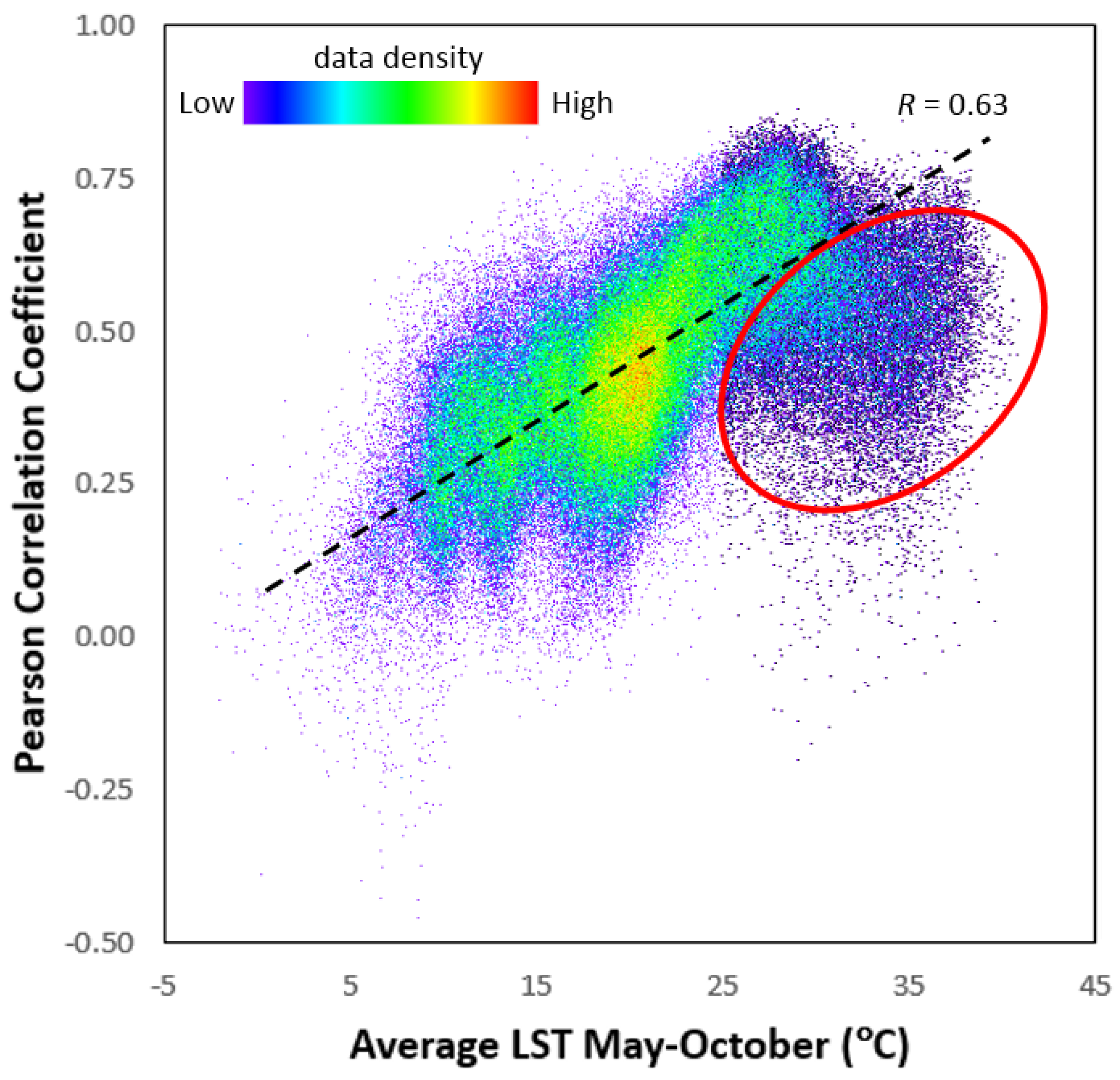This subdivision suggests some sort of connection between the R values and the magnitude of LST, considering that these three zones are commonly characterized by decreasing values in the average LST, with the Mediterranean areas being the warmest and the Scandinavian Peninsula being the coldest. Starting from this consideration, a scatterplot between the R values and the corresponding warm season average LST is presented in Figure 4, with the aim of investigating the actual existence of a connection between the magnitude of the observed LST (which is a proxy of the climatic condition of the site) and its capability to capture the SM dynamic and to explain the spatial variability of the obtained R values.

Figure 4. Scatterplot between the soil moisture (SM) vs. LST Pearson correlation coefficients (see Figure 2a) and the warm season (May to October) average LST values. The colors represent the density of the data in the scatterplot, which increases from purple/blue to green to yellow/red.

Figure 4. Scatterplot between the soil moisture (SM) vs. LST Pearson correlation coefficients (see Figure 2a) and the warm season (May to October) average LST values. The colors represent the density of the data in the scatterplot, which increases from purple/blue to green to yellow/red.

The data in Figure 4 indeed show a linear trend of increasing R values with season-average LST (correlation coefficient of 0.63), which is true for most of the cells in the domain. The lowest R values in the coldest areas may be explained again by the effects of the likely presence of snow, at least during a fraction of the analyzed period. Of greater interest is the decrease of correlation for the very high average LST, which is represented by the cloud of points that diverge from the main linear trend (as marked by the red circle in Figure 4); this behavior (which pulls down the slope of the linear regression for the highest values) may be explained by a saturation effect in SM during very dry conditions. In fact, the highest LST values are generally observed on dry bare soil or sparsely vegetated zones, where LST continues to rise (unbounded variable) even after the soil moisture has reached the residual value (bounded variable).

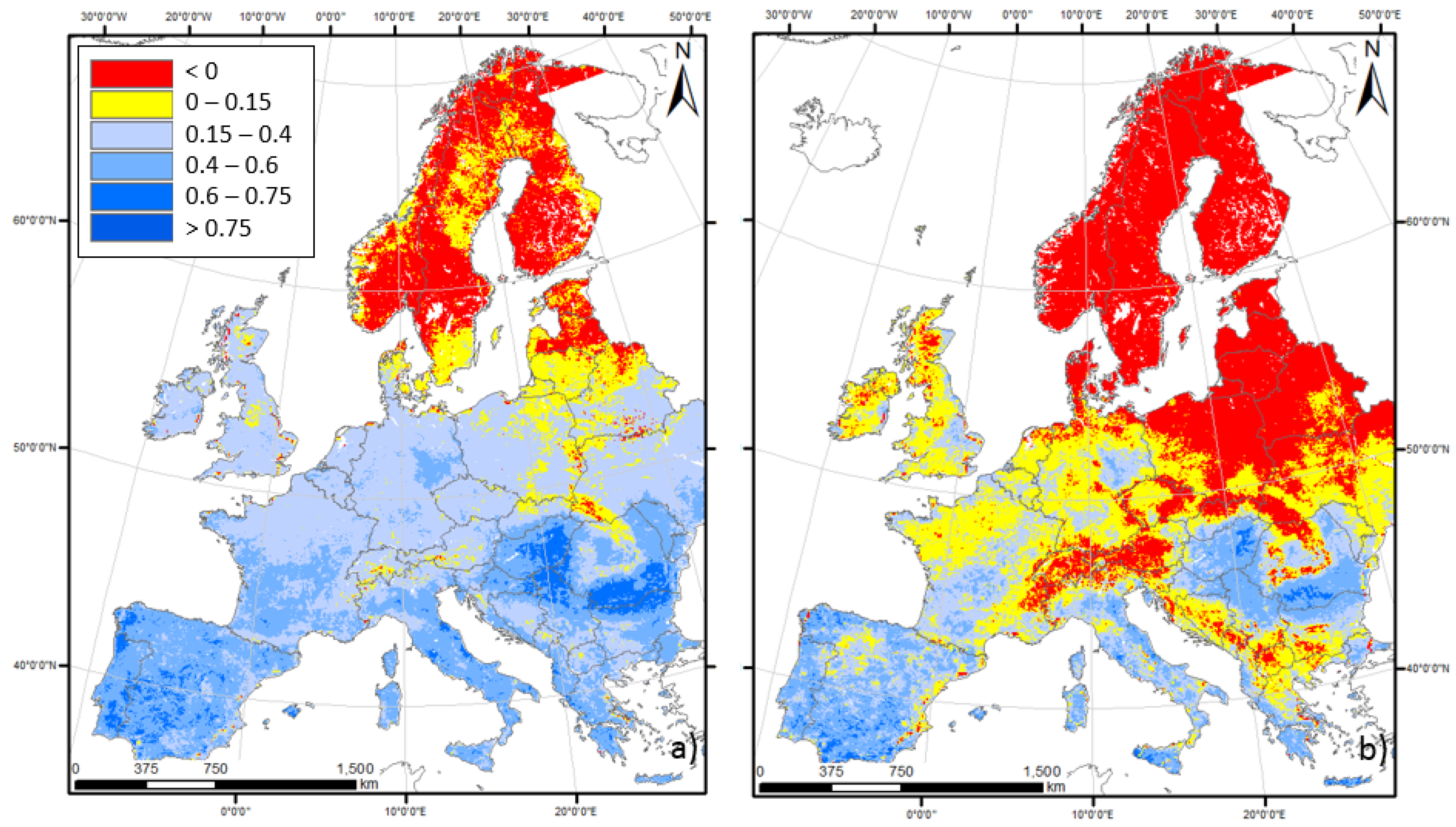
The assumption that focusing on the warm season only would reduce the negative impact of snow coverage on the thermal regime is verified by the maps of R values reported in Figure 5, in which the correlation between the anomalies of SM and LST are computed on the whole year (Figure 5a) and the cold season only (Figure 5b). The map computed using the data from the full year shows a general reduction of the R values compared to the warm season-only ones (see Figure 2a), which becomes more marked on the northern domain where several negative values can be observed (direct relationship between SM and LST); however, it is not surprising that a decrease of SM is associated with a decrease of LST over those areas, since they are the ones mostly covered by snow during winter time. The spatial distribution of the R values obtained for the cold season (Figure 5b) shows a further reduction and confirms a subdivision of the domain in two macro areas, a North-East part with negative values and a South-West part with positive values.

Figure 5. Spatial distribution of the Pearson correlation coefficient (R) between soil moisture and land surface temperature anomalies computed on monthly data for: (a) the full year; and (b) the cold season, for the period 2001–2013. Values in yellow and red are not significant at p = 0.05.

Figure 5. Spatial distribution of the Pearson correlation coefficient (R) between soil moisture and land surface temperature anomalies computed on monthly data for: (a) the full year; and (b) the cold season, for the period 2001–2013. Values in yellow and red are not significant at p = 0.05.

It is worth pointing out that across Central Europe both negative and positive values can be observed. These results highlight the more complex behavior of the SM-LST relationship when the full year is analyzed, making the derivation of a common approach for the use of LST as proxy of SM less straightforward. Given that the direct inverse relationship holds for most of the domain when the warm season is considered, we keep the analysis focused on these data only, following the consideration that this period is the one of greatest interest for ecosystem drought analyses.

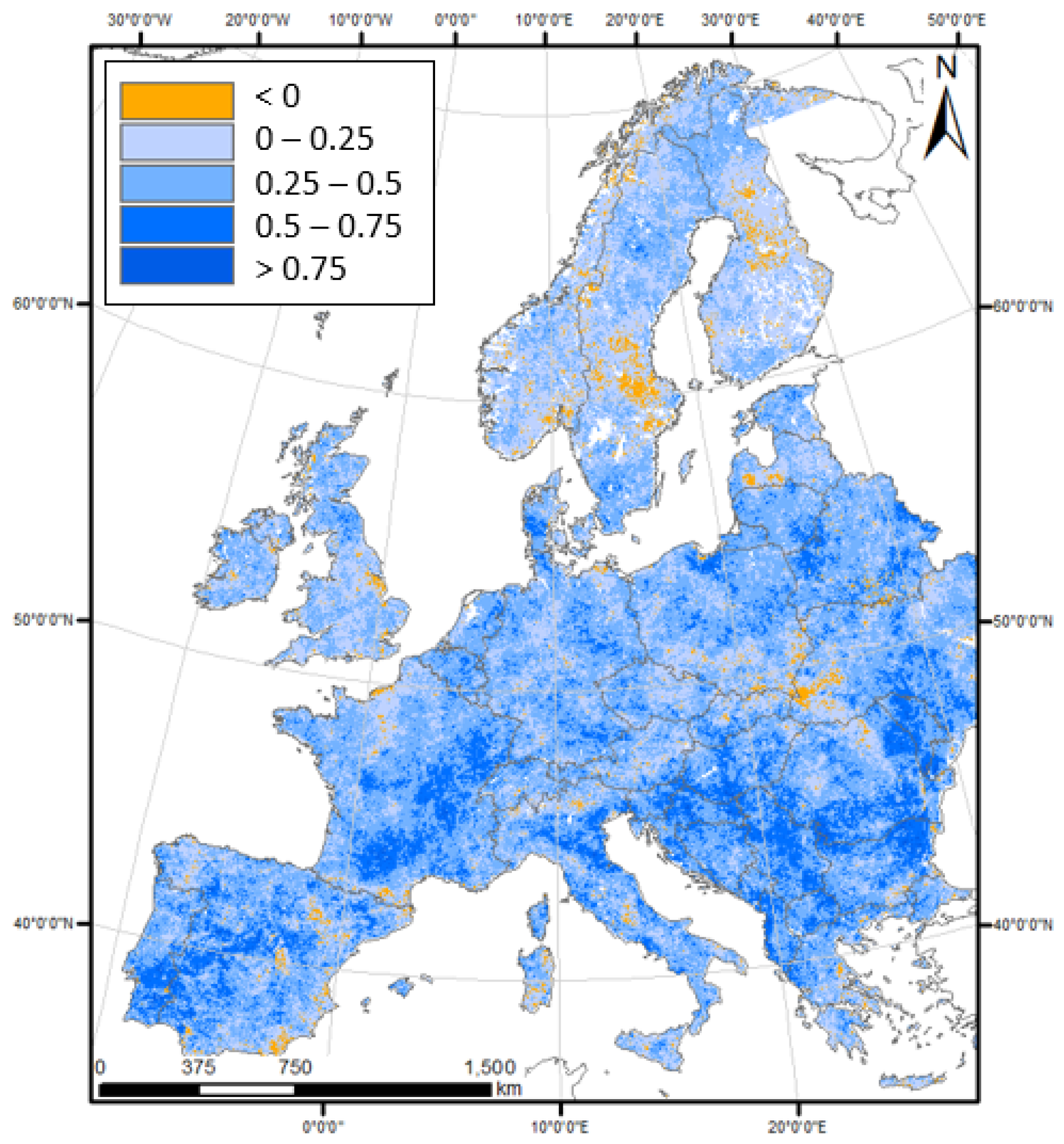
Following the analyses of the capability of LST to explain large parts of the dynamic in SM, a more specific focus on the occurrence of SM dry extremes (z_SM > 1) is achieved by means of the analysis of the indices derived from the contingency table. The map in Figure 6 presents the HSS for the dry extremes and demonstrates the skillfulness of the LST model in reproducing the dry extremes observed in the SM time-series. The color scheme is chosen to highlight the areas with no skill (compared to the random reference case) in orange, whereas the different degrees of skillfulness are depicted in blue shades.

Overall, the LST model is demonstrated to be skillful over most of the domain (about 98%), with an average value of 0.35 ± 0.15; also in this case it is possible to notice a greater abundance of high values in the southern part of the domain (i.e., South France, West Iberia, and Balkan countries), even if there is no clear distinction in three sub-zones as in the case of correlation values. The no skill values are clustered over few locations scattered all over the domain, with two larger clouds in South Sweden and Ukraine, which show some similarities with the correlation map in Figure 2a.

As pointed out in several studies, the HSS (similarly to most of the skill scores) tends to approach zero when either the events or the non-events are predominant [38], even if HSS, unlike other indices, still gives weight to the correct modelling of non-events [39]. This is the case of rare events such as droughts, even if the non-strict definition of an event used in this paper (z_SM > 1) should partially reduce the problem. Assuming as a rule of thumb a value of HSS of 0.33 as a minimum target for our model, indicating that the model predicts a minimum of 1/3 of the non-randomly predictable events correctly, in our study about 50% of the domain respect this target as exemplified by the average value reported above. This indication can be useful as a benchmark for future comparisons of other indices against this one.

Figure 6. Spatial distribution of the Heidke Skill Score (HSS) computed between ensemble SM (observation) and LST (model) anomalies for the “events” z_SM > 1 (dry extremes). Values in orange identify no skill for the LST model.

Figure 6. Spatial distribution of the Heidke Skill Score (HSS) computed between ensemble SM (observation) and LST (model) anomalies for the “events” z_SM > 1 (dry extremes). Values in orange identify no skill for the LST model.

Since HSS summarizes the LST capability to reproduce both events and non-events, a more specific focus only on the events may be of interest for a near-real-time drought monitoring system. With this aim, two different indices are mapped in Figure 7, focusing on the probability to detect an observed event (POD, Figure 7a) and on the probability to obtain a false alarm from the LST model (POFD, Figure 7b). Given that the meaning of the two indices is the opposite (1 is the best score for POD whereas it is the worst score for POFD), we inverted the two color-bars in order to simplify the cross-comparison of the two maps.

The POD maps show some similarities with both R and HSS maps, with higher values on the southern part of the domain. On average, POD assumes values in the range 0.66 ± 0.11, meaning that 2 of the SM observed events out of 3 are correctly modelled by the LST. This probability increases to around 80% in the Mediterranean and East European areas, whereas it decreases to around 50% in Northern Europe. The interpretation of the spatial distribution of POFD values results is more complex since no clear spatial patterns can be observed. On average, the POFD is equal to 0.31 ± 0.08, suggesting that one out of three of the LST-detected events can be a false alarm. This information, complementary to the previous one, provides an overall overview of the reliability of an event detected by a drought monitoring system based on LST anomalies, as well as on the ability of this system to actually capture the events that would be identified by a similar system based on SM anomalies. Finally, it is worth highlighting that both the POD and POFD, as well as the HSS, of the ensemble SM anomalies against the events derived from the in situ measurements were close to the values obtained in this study on the LST against the ensemble SM itself (see [22]).

Figure 7. Spatial distribution of the Probability of: (a) Detection (POD); (b) False Detection (POFD), computed between ensemble SM (observation) and LST (model) anomalies for z_SM > 1 (dry extremes).

Figure 7. Spatial distribution of the Probability of: (a) Detection (POD); (b) False Detection (POFD), computed between ensemble SM (observation) and LST (model) anomalies for z_SM > 1 (dry extremes).

4. Summary and Conclusions

In this paper we evaluated the capability of remotely sensed land surface temperature (LST) and derived quantities to represent a proxy of modelled soil moisture (SM) over Europe, with the aim of using LST within the context of a near-real time drought monitoring system. Given that the three-model ensemble SM dataset used here as a benchmark has been demonstrated to be a valuable tool for drought monitoring, it is interesting to understand the potential contribution of LST as an auxiliary source of information in an integrated monitoring system without involving complex modelling based on LST.

The use of LST anomalies as derived from the monthly MODIS product (MOD11C3) showed a good ability to capture the dynamic of SM over continental Europe, with most of the domain (about 92%) characterized by significant correlation coefficients at p = 0.05. The results of the correlation analysis show higher values over the Mediterranean region and the worst performance in Scandinavia and mountainous areas (Alps, Carpathians, Pyrenees); these latter are mainly related to the difficulties in properly capturing the water dynamics over steep areas, as well as to the effects of the likely presence of snow coverage on the surface thermal regime.

The LST anomalies clearly outperformed the other LST-derived quantities in reproducing the SM dynamics, including the air-to-surface temperature gradient (ΔT) and the day-night LST difference (ΔLST). These results suggest that even if ΔT and ΔLST are conceptually more suitable for a direct modelling of the magnitude of SM or evapotranspiration (ET) fluxes, the lower informative content of nighttime temperature and air temperature compared to daytime LST reduces the power of ΔT and ΔLST compared to the use of simple LST. It is interesting to point out how ΔT and ΔLST perform quite closely, even if nighttime surface temperature and daytime air temperature were derived from two distinct data sources (MODIS data the former and interpolation of ground data the latter).

The LST anomalies also proved to be a good model to reproduce SM dry extreme events (anomalies greater than 1), as quantified by the Heidke Skill Score (HSS). This index demonstrated that LST is skillful in capturing the SM dry extreme events in almost the whole domain (about 98%), with an average skill that is well above zero (0.35 ± 0.15), indicating that a minimum of 1/3 of the non-randomly predictable events are captured thanks to the use of LST. This result is more significant if we consider that for rare events, as droughts, skill indices tend to be very low.

As a further detailing of the analysis on dry extremes, the spatial distribution of the Probability of Detection (POD) and the Probability of False Detection (PFD) has been investigated; these indices highlight the capability of LST to detect, on average, 2/3 of the observed SM dry events, accompanied by a 30% chance of obtaining a false alarm. The spatial distribution of the POD shows a clear concentration of the highest values in the Southern part of the domain, where a higher chance of correctly detecting an event is observed (around 80%), whereas the frequency of false alarm is somehow consistent across the whole domain.

Overall, these data suggest that the use of LST as proxy of SM is promising even when it is directly used for estimating monthly anomalies, avoiding the involvement of complex modelling or further auxiliary information. The results reported in this study confirm that the use of LST is quite reliable over South Europe, where correlation, skill, and capability to detect dry events show the highest values. However, a limited capability of LST to predict SM was also observed over extremely dry conditions (i.e., season average LST > 32–35 °C), tightening the optimal conditions of applicability to water controlled systems with a moderate degree of stress. Over North Europe (i.e., Scandinavian Peninsula) the value of LST is more limited, likely due to the effects of snow coverage on the surface thermal regime, as well as a more complex modelling of the hydrological cycle due to snow melting phenomena.

The results reported in this study can provide a sort of benchmark for future studies on the use of remotely sensed LST for SM and ET estimations at a continental scale over Europe; in fact, more complex methodologies that take advantage of LST as just one of a larger set of input data (i.e., surface energy balance models, semi-empirical methods) should take the outcomes of this study as a minimum target for a quality assessment of the model performance. Any additional processing of LST data should add a significant amount of value compared to this case in order to justify its use in practical applications for drought monitoring.