Satellite Image Time Series Decomposition Based on EEMD

Abstract

Satellite Image Time Series (SITS) have recently been of great interest due to the emerging remote sensing capabilities for Earth observation. Trend and seasonal components are two crucial elements of SITS. In this paper, a novel framework of SITS decomposition based on Ensemble Empirical Mode Decomposition (EEMD) is proposed. EEMD is achieved by sifting an ensemble of adaptive orthogonal components called Intrinsic Mode Functions (IMFs). EEMD is noise-assisted and overcomes the drawback of mode mixing in conventional Empirical Mode Decomposition (EMD). Inspired by these advantages, the aim of this work is to employ EEMD to decompose SITS into IMFs and to choose relevant IMFs for the separation of seasonal and trend components. In a series of simulations, IMFs extracted by EEMD achieved a clear representation with physical meaning. The experimental results of 16-day compositions of Moderate Resolution Imaging Spectroradiometer (MODIS), Normalized Difference Vegetation Index (NDVI), and Global Environment Monitoring Index (GEMI) time series with disturbance illustrated the effectiveness and stability of the proposed approach to monitoring tasks, such as applications for the detection of abrupt changes.

1. Introduction

With the development of satellite technology, the amount of historical remote sensing data is growing. These long sequences of remote sensing data, which are called Satellite Image Time Series (SITS), contain a considerable amount of information, such as land-cover dynamics and disturbances. SITS are always considered valuable resources for Earth monitoring [1]. Thus, the study of the information of changing patterns, scope, scale, and trends is very meaningful but challenging work.

SITS usually contain seasonal, trend, and remainder components [2]. Seasonal and trend components are key elements for SITS analysis because they contain important information for understanding Earth science processes. Seasonal components constitutionally reflect inter-annual periodic fluctuations that are usually driven by the annual temperature, weather, seasons of the year, or growth cycles of vegetation [3]. Trend components mainly reflect long-term changes. Hence, decomposing SITS into different components, especially the seasonal components and trend components, plays an important role in SITS analysis. Various techniques were investigated for this purpose (see Kandasamy et al. [4] for a review). For example, Jönsson and Eklundh [5] extracted seasonal information based on nonlinear least-squares fits of asymmetric Gaussian model functions. A logistic piecewise model was used by Zhang et al. [6], and a quadratic model was used by de Beurs and Henebry [7]. Eastman et al. [8] introduced the Seasonal Trend Analysis (STA) method based on harmonic analysis. Parmentier and Eastman [9] extended this method using multivariate time series via segmentation.

These methods decompose the seasonal components into a set of predefined functions, which simplifies the seasonality comparison across different years. Cleveland et al. [10] proposed a classic and effective seasonal-trend decomposition model called the Seasonal-Trend decomposition process based on Loess (STL). However, this method is not fully automated and a set of parameters must be manually set to guarantee the performance.

The fitting methods depend on their parameters and may cause some useful information to be smoothed. A better strategy for decomposition is based on the inherent nature of the data. Singular Spectrum Analysis (SSA) is a subspace-based method that decomposes time series based on the inherent oscillation of data [11], especially for decomposing time series into different oscillatory components without fitting. Mahecha et al. [12] applied SSA to decompose the remote-sensed fraction of Absorbed Photosynthetically Active Radiation (fAPAR) time series into different frequencies, including seasonal components. SSA was also employed by Forkel et al. [13] to estimate trend component on seasonal-adjusted Normalized Difference Vegetation Index (NDVI) time series. One of the drawbacks of SSA is that its performance depends on the choice of the window length. Furthermore, it needs extra work to choose a combination for a specific oscillation component because the decomposition result depends not on the time scale but the eigenvalues.

In this study, we note the fact that the seasonal component varies at or near the seasonal frequency (i.e., one cycle per year), while the trend component is the low-frequency variation along with non-stationary long-term changes in levels. Both the seasonal and trend components were correlated with frequency. Thus, we mainly focused on how to extract these two components efficiently and automatically based on the time frequency analysis and proposed a framework of decomposing SITS based on Ensemble Empirical Mode Decomposition (EEMD). EEMD [14] was first presented to improve upon the original Empirical Mode Decomposition (EMD). It is capable of decomposing any complex signal into a series of orthogonal components called Instinct Mode Functions (IMFs). Accordingly, the motivation for us is to employ EEMD for decomposing SITS into IMFs and to choose relevant IMFs to represent seasonal and trend components. We used 16-day composite Moderate Resolution Imaging Spectroradiometer (MODIS) NDVI [15] time series and 16-day composition of Global Environment Monitoring Index (GEMI) [16] time series with fire disturbance to validate the effectiveness of the proposed framework.

The organization of the paper is as follows. Section 2 details the two-stage decomposition method and the proposed strategy. Section 3 provides the experimental data and the application for detecting abrupt changes according to the proposed method. Section 4 addresses several concluding remarks and provides an outlook for future work.

2. Proposed Framework

The proposed framework contains a two-stage process to decompose SITS. In the first stage, EEMD is employed for decomposition to obtain a series of IMFs. Then, the selected IMFs are adopted to construct seasonal and trend components.

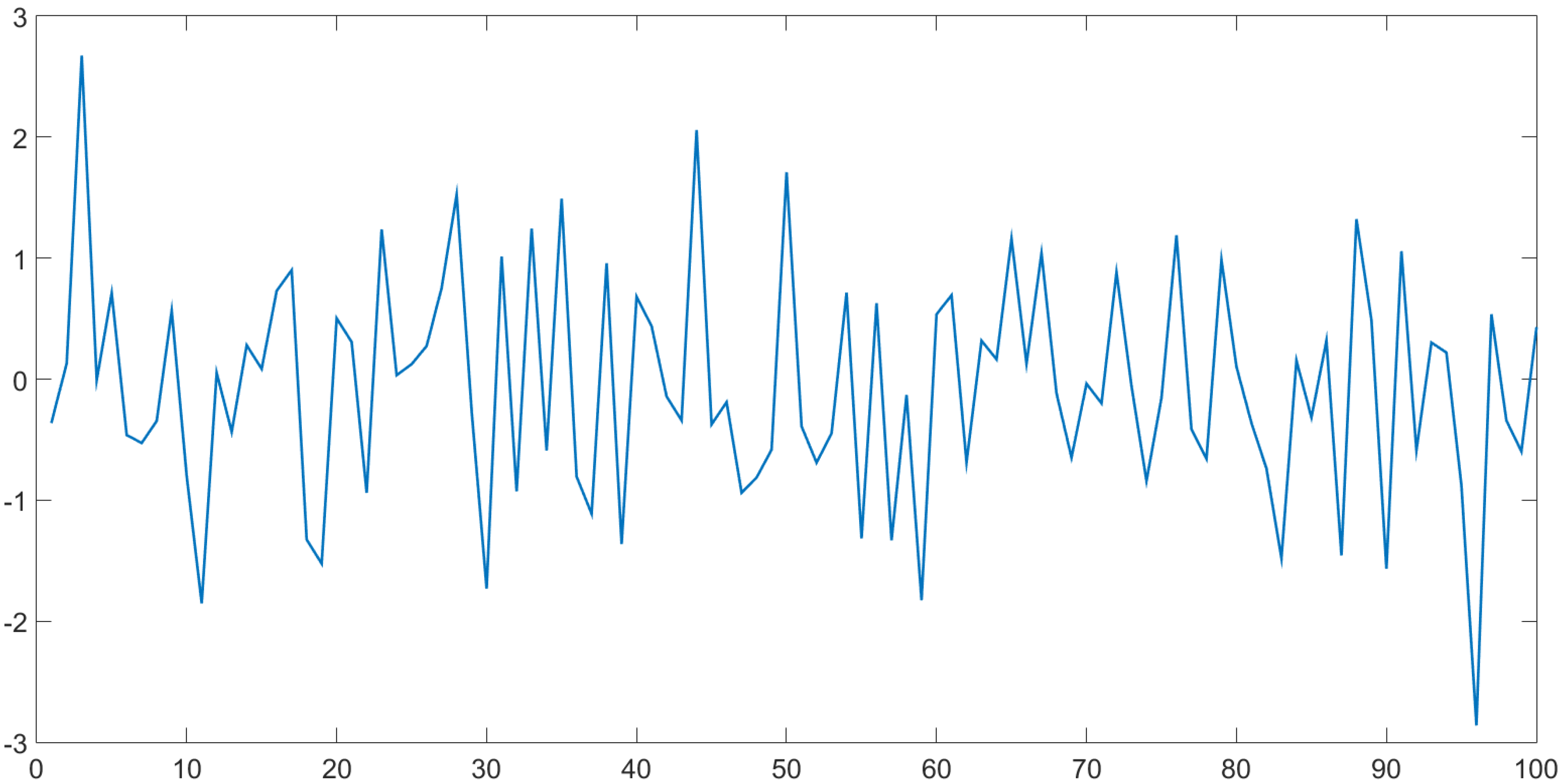
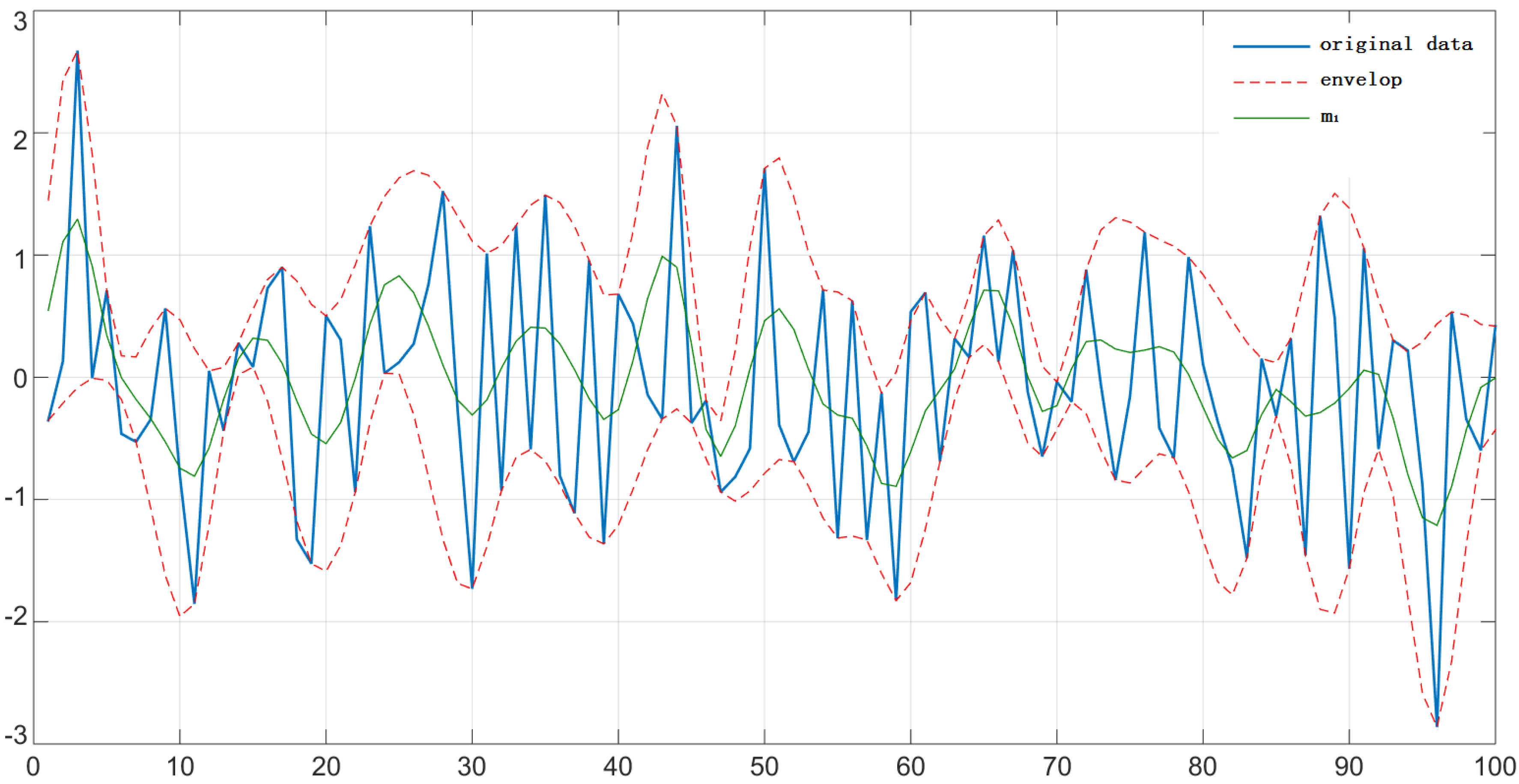
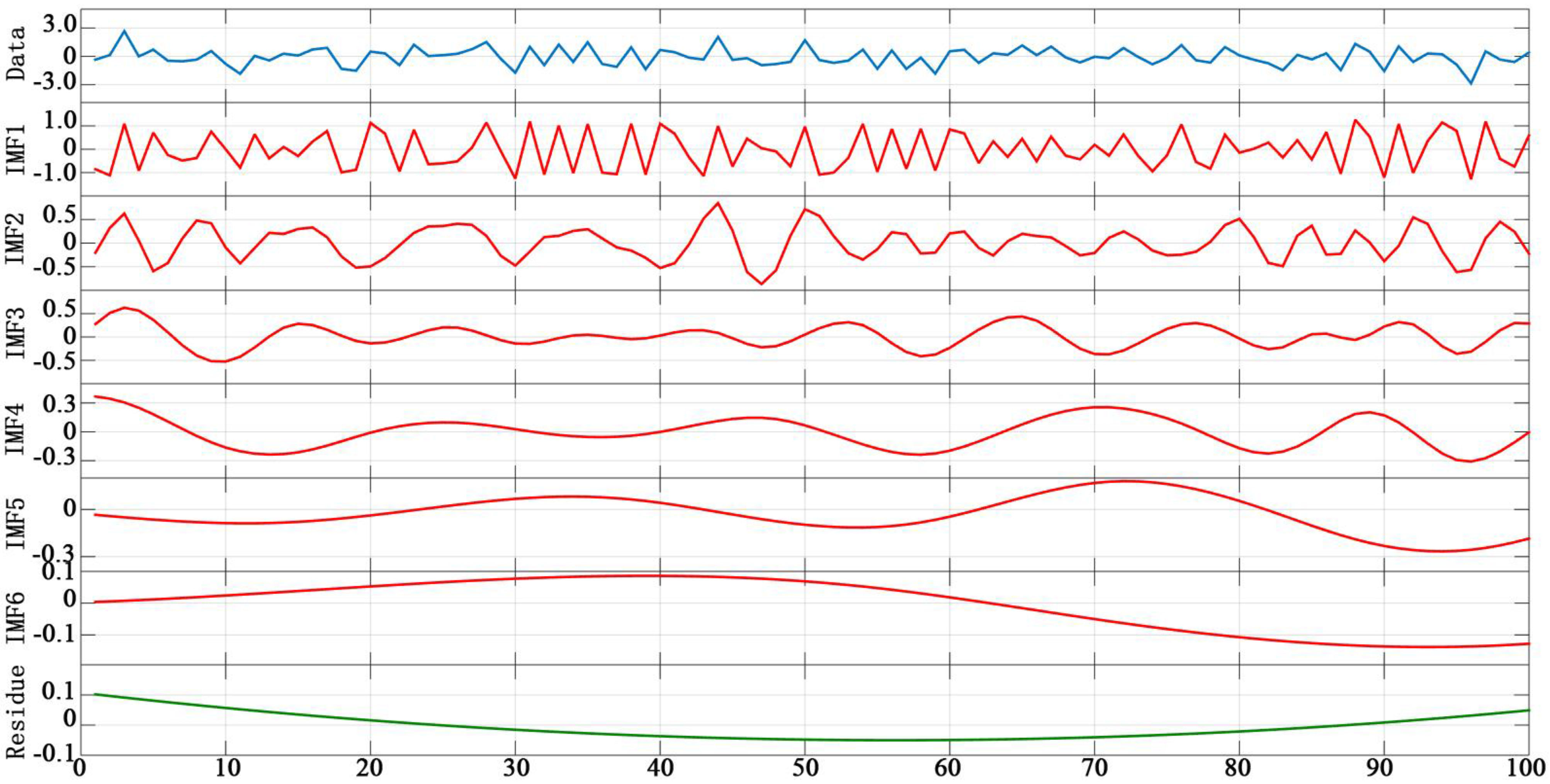
2.1. Ensemble Empirical Mode Decomposition

Before introducing EEMD, a brief introduction to EMD is provided here. EMD is a fundamental part of the classic Hilbert-Huang Transform (HHT) [17], which has been successfully applied in many research areas [18,19,20]. EMD relies on the decomposition of the signal under study into IMFs and a residue [17]. Each IMF stands for an oscillatory mode of the original data, and the residue stands for the overall trend. The process of extracting IMF is called sifting, which defines a local characteristic time scale of the data as the time interval of two adjacent extremes. Based on the local time scale, the algorithm extracts a finite number of IMFs whose frequencies range from high to low. Here, we define a random time series x(t), as shown in Figure 1, and the sifting process can be described as follows.

Step 1. In x(t), the upper envelope represents all the local maxima using a cubic spline line, and the lower envelope is used to connect all the local minima. The mean SITS of the upper and lower envelopes is denoted as m₁(t) as shown in Figure 2.

Step 2. Mean envelope m₁(t) is subtracted from x(t) to approximate an IMF, as:

$$h_1(t)=x(t)-m_1(t)$$

(1)

Step 3. View h₁(t) as a new time series, and step 1 and step 2 are repeated until the following stop criterion is satisfied.

$$\begin{array}{l}{h}_2(t)=h_1(t)-m_2(t)\\ \mathrm{...}\\ h_k(t)=h_{k-1}(t)-m_k(t)\end{array}$$

(2)

Huang et al. [17] further determined a stop criterion using a Cauchy type of convergence test:

$$S{D}_k=\frac{{\displaystyle {\sum }_{t=0}^T{\left|h_{k-1}(t)-h_k(t)\right|}^2}}{{\displaystyle {\sum }_{t=0}^T{h}_{k-1}^2(t)}}$$

(3)

If $S{D}_k$ is smaller than a predetermined value, the sifting process is stopped, and the highest frequency component of the data is designated as the first IMF:

$$c_1(t)=h_k(t)$$

(4)

Step 4. After the highest frequency IMF is extracted, we subtract c₁ from the rest of the data:

$$r_1(t)=x(t)-c_1(t)$$

(5)

Step 5. From the residue r₁, we can extract the second highest frequency IMF c₂ and residue r₂ by the sifting process described above. Similarly, all the IMFs c_i can be repeatedly extracted from high to low frequency, level by level:

$$\begin{array}{l}{r}_2(t)=r_1(t)-c_2(t)\\ \mathrm{...}\\ r_i(t)=r_{i-1}(t)-c_i(t)\end{array}$$

(6)

When residue r_i becomes a monotonic function and there are no more IMFs that can be extracted, the process stops. Finally, the time series is decomposed as:

$$x(t)={\displaystyle {\sum }_{i=1}^n{c}_i}(t)+r_n(t)$$

(7)

Ideally, a signal is considered an IMF if it satisfies two conditions, namely: (1) the number of extremes and the number of zeros crossing must either be equal or differ by one at most, and (2) the mean value of the upper and lower envelopes must be zero. In fact, the sifting process cannot obtain a perfect IMF. It is an approximation of an IMF with repeated siftings. However, EMD has the drawback of leading to the “mode mixing” problem [14], which indicates the presence of oscillations of extreme disparate amplitudes and scales in a mode or presence of extreme similar oscillations in different modes. The motivation for us to employ EEMD is summarized as follows: (1) for SITS, the “mode mixing” problem may be more serious, as various noise and clouds cover the Earth’s surface in satellite images, which may obscure the data, while EEMD effectively resolves it via an ensemble of the signal by adding noise, and (2) EEMD is capable of avoiding single IMF, including multiple oscillation components with dramatically disparate time scales, simultaneously preventing components with similar time scales from being included in different IMFs. The key difference between EEMD and EMD is that EEMD incorporates Gaussian white noise into the original time series to uniformly distribute the entire time series in different scales to avoid mode mixing. Due to the randomness of white noise, the additive noise can be reduced in the mean of the corresponding IMFs by sufficient repeated trials. EEMD has better performance than EMD [21,22] and has been widely applied [23,24,25].

The description of the EEMD algorithm is addressed below.

Step 1. A random white noise series w_m(t) is added to the original time series x(t):

$$x_m(t)=x(t)+w_m(t)$$

(8)

Step 2. x_m(t) is decomposed by EMD:

$$x_m(t)={\displaystyle {\sum }_{i=1}^n{c}_{i,m}(t)+r_{i,m}(t)}$$

(9)

Step 3. Step 1 and Step 2 are repeated M times with different white noise series.

Step 4. The means of the corresponding IMFs are calculated:

$$c_i(t)=\frac{1}{M}{\displaystyle {\sum }_{m=1}^M{c}_{i,m}(t)}$$

(10)

It is clearly observed that in each trial of EMD, the noise is added, leading to a data analysis robust against noise, and EEMD treats the average of the ensembles of EMD as the optimum choice of IMFs. Figure 3 illustrates the decomposition results of EEMD using the random time series shown in Figure 1. In this experiment, we employ white noise of an amplitude 0.2 times the standard deviation of the original data and 100 trials for EEMD, as recommended in the existing literatures [14,26].

Figure 1. An example of a random time series.

Figure 1. An example of a random time series.

Figure 2. For the above random time series (blue line), the upper and lower envelopes (dot-dashed lines) and the mean curve (green line) are provided.

Figure 2. For the above random time series (blue line), the upper and lower envelopes (dot-dashed lines) and the mean curve (green line) are provided.

Figure 3. For the above random time series, an illustration of the decomposed components using Ensemble Empirical Mode Decomposition (EEMD) is provided. The original time series (blue line) is decomposed into six Intrinsic Mode Functions (IMFs) (red line) and a residue (green line).

Figure 3. For the above random time series, an illustration of the decomposed components using Ensemble Empirical Mode Decomposition (EEMD) is provided. The original time series (blue line) is decomposed into six Intrinsic Mode Functions (IMFs) (red line) and a residue (green line).

2.2. EEMD for SITS

As shown in Figure 3, different IMFs from various time-frequency domains can be extracted. For example, IMF1 contains the highest frequency and always represents the noise [27].

Wu and Huang [28] implemented numerical experiments on white noise time series. They found that for the IMFs of white-noise series, the energy density ${\overline{E}}_k$, and the averaged period ${\overline{T}}_k$ can be expressed as:

$$\ln {\overline{E}}_k+\ln \left\{{\overline{T}}_k\right\}=const$$

(11)

where ${\overline{E}}_k$ represents the energy density and ${\overline{T}}_k$ means the average period. The energy density function is ${\chi }^2$-distributed. They further established a test method to assign the statistical significance of an IMF for noisy data. Figure 4 illustrates the statistical significance test for the IMFs in Figure 3. The green dots from left to right on the x-coordinate illustrate the energy density as a function of the averaged period of IMFs 1 to 6. The green dots closer to the red line indicate that the IMFs are closer to the Gaussian white noise. From the results, it is verified that IMF1 is the closest to the noise. As a consequence, IMF1 is usually subtracted from the original time series when extracting seasonal and trend components.

Figure 4. Statistical significance test between the energy density and the averaged period. Note that the green dots from left to right show the energy density as a function of the averaged period.

Figure 4. Statistical significance test between the energy density and the averaged period. Note that the green dots from left to right show the energy density as a function of the averaged period.

2.2.1. Seasonal Component Extraction

In SITS, the crucial characteristic of the seasonal component is that it has a regular cycle (i.e., one cycle per year). For geographic data, the seasonal cycle is usually one year. Thus, we considered the IMF with a one-year period cycle as the seasonal component, but it this was not always true for SITS. Sometimes there were oscillations with a double peak in a year (an example is shown in Section 3.1). Therefore, more IMFs are needed to express the seasonal component in SITS:

$$S={\displaystyle \sum _{i=b}^c{c}_i(t)}$$

(12)

where the c-th IMF has an oscillation of one year, the b-th to the c-th IMFs have annual cycles, and b may be identical to c when there is just one IMF containing annual variation. This is similar to a band pass filter based on EEMD. Three steps are needed for choosing IMFs.

Step 1. Seasonal averaged data are obtained by calculating the periodical average of the time series data. Take one particular time series as an example, which consists of data over 10 years. One oscillation was acquired by averaging the values of 10 years, and the averaged seasonal data were obtained by duplicating the oscillation over 10 years.

Step 2. The seasonal averaged dataset generally represents one average oscillation of all periodic oscillations, and it also represents the most fundamental and consistent oscillations of all periods. Accordingly, we obtained the IMFs of this fundamental oscillation by decomposing the seasonal average data acquired in Step 1 using EEMD.

Step 3. We selected the IMFs of the decomposition outcome of the original series corresponding to the IMFs of the seasonal averaged model to formulate the actual seasonal term.

2.2.2. Trend Component Extraction

In [27], Wu et al. noted that the most common trend component was extrinsic and predetermined and gave an intrinsic and adaptive trend definition for nonlinear and non-stationary data: “The trend is an intrinsically fitted monotonic function or a function in which there can be at most one extremum within a given data span” [14]. The residue of EEMD is a monotonic function that intrinsically presents the overall trend of a time series. Trends are also generated with different time scales using the sum of the IMFs, which present oscillations for multiple years as well as the residue [27]. Therefore, the trend component generated from EEMD satisfies this definition and can be expressed as:

$$T={\displaystyle \sum _{i=a}^n{c}_i(t)}+r(t)$$

(13)

where the IMFs with frequency lower or equal to the a-th IMF are selected to add to the residue to construct the trend. The selection of a is affected by the time scale of the trend and is flexible according to the need of the application.

The seasonal-trend decomposition method can be summarized as follows.

Step 1. Decompose the original SITS by EEMD introduced in Section 2.1.

Step 2. Subtract IMF1 from the original SITS to de-noise SITS.

Step 3. Decompose the periodical average of the time series data obtained from Step 2 by EEMD, select the IMF component corresponding to the decomposition outcome from Step 1, and construct the seasonal component using Equation (12).

Step 4. Construct the trend component with Equation (13).

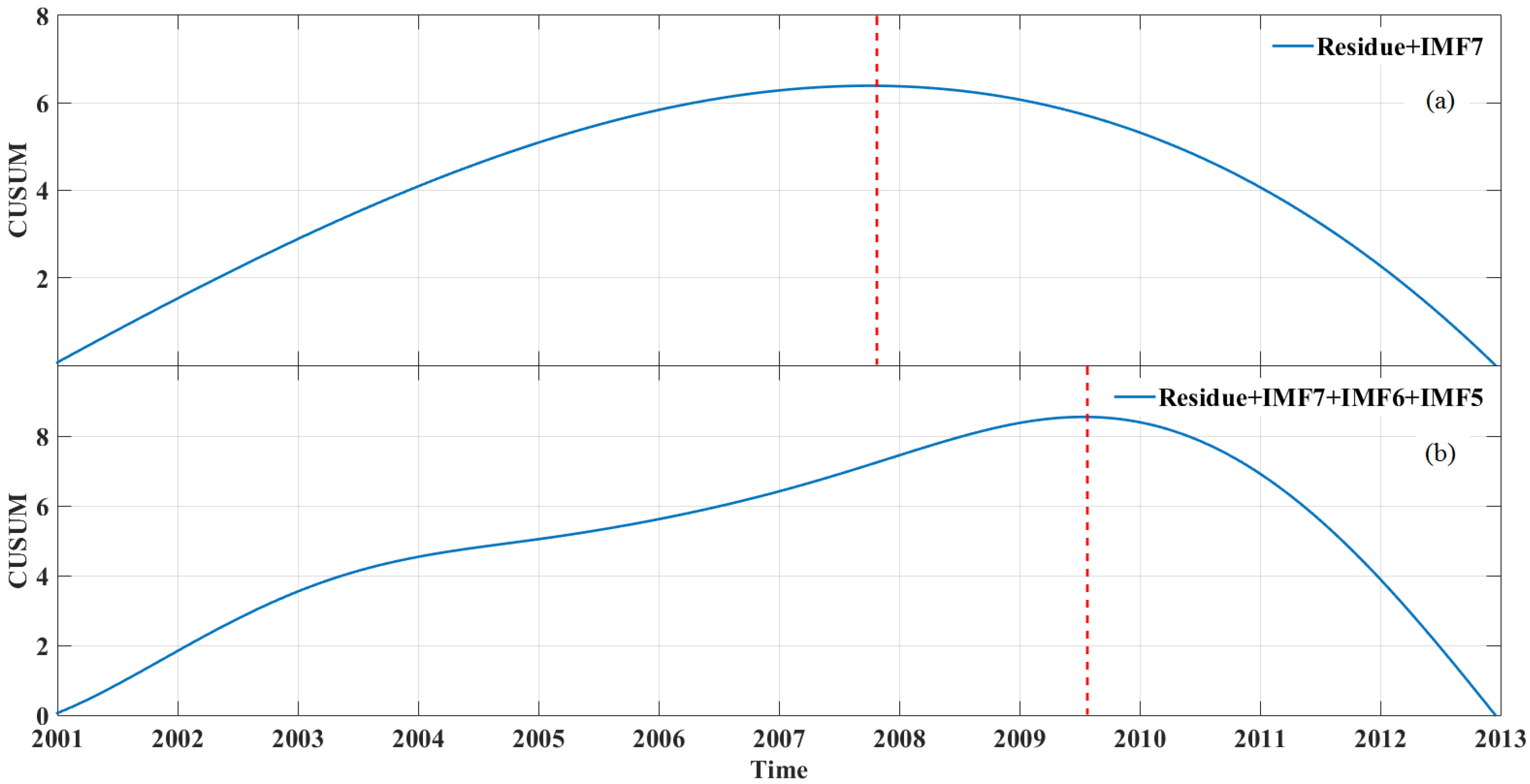
2.2.3. Trend Component for Change Detection

In this subsection, we aim to apply the extracted trend component for abrupt change detection. Theoretically, high-frequency IMFs are required to increase the accuracy of the change detection. However, based on the analysis in Section 2.2.2, high-frequency IMFs may bring strong waves, which lead to false change detection that obscures the real change point rather than increasing the detection accuracy. Hence, the trend component formulation for disturbance detection via the incorporation of high-frequency IMFs should seek to limit the strong waves of IMFs. In this work, the selection of IMFs is based on the intensity of the IMF wave [29], evaluated by calculating the IMF wave energy:

$$G_i={\displaystyle \sum _{t=1}^N{c}_i^2(t)}$$

(14)

where c_i(t) represents the i-th IMF and G_i represents the IMF wave energy, which is the aggregation of the mean deviations of the series elements. Clearly, the energy increases proportionally to the wave intensity. For the residue r(t) of a nonzero-mean series, the energy G^r can be further defined as:

$$G^r={\displaystyle \sum _{t=1}^N[r(t)-m^r]}2$$

(15)

where

$$m^r=\frac{1}{N}{\displaystyle \sum _{t=1}^{N}r(t)}$$

(16)

The use of intensity to limit the strong waves can avoid the incorrect detection of the positions of change points. In addition, if there is no change, the energy of the residue will be small. Higher-frequency IMFs are not added to construct the trend component with the limitation, and false change points will not be detected.

To achieve an effective trend component for change detection purposes, we implement the following two steps:

Step 1. Calculate the energy of the residue using Equation (15), and empirically set the threshold as the residue energy ratio (less than 1).

Step 2. Calculate the wave energy using Equation (14) from the IMF with the lowest frequency. If the energy is no greater than the threshold, then the wave intensity is less than the ratio of the residue wave, and its variation does not obscure the structural variation in the residue. Accordingly, this IMF is added to the residue and formulates the trend component. These steps are repeated using the IMF with infra-low frequency until the energy of this IMF is greater than the threshold. Finally, the resulting trend component, which only contains IMFs with low frequency and energy, is taken as the output.

3. Experiment and Discussion

Field Study: The study area is located in the Yinan River Forest in the northeast of Heilongjiang Province, China. A disastrous fire occurred in this area on 27 April 2009 and was not put out until 2 May 2009. Figure 5 shows a false-color-composite image of Landsat TM shot on 23 May 2009 of the burned area. In this experiment, SITS were generated from MODIS 250 m 16-day composite gridded vegetation index products (MOD13Q1) from 1 January 2001 to 31 December 2009. We converted the original data to a projection of WGS 84/UTM zone 52N.

Experiment Setup: We first validated our decomposition model by a 16-day composition NDVI time series of forest type. SITS were collected from a normal region (denoted as yellow block 1 in Figure 5), which was used to illustrate and discuss the time series decomposition procedure. Second, the decomposition mode was validated by a 16-day composition GEMI time series with disturbance. In this experiment, SITS were from a burned area (yellow block 2 in Figure 5), which was used to detect the fire disturbance, and we also analyze a method of selecting IMFs to generate the trend component.

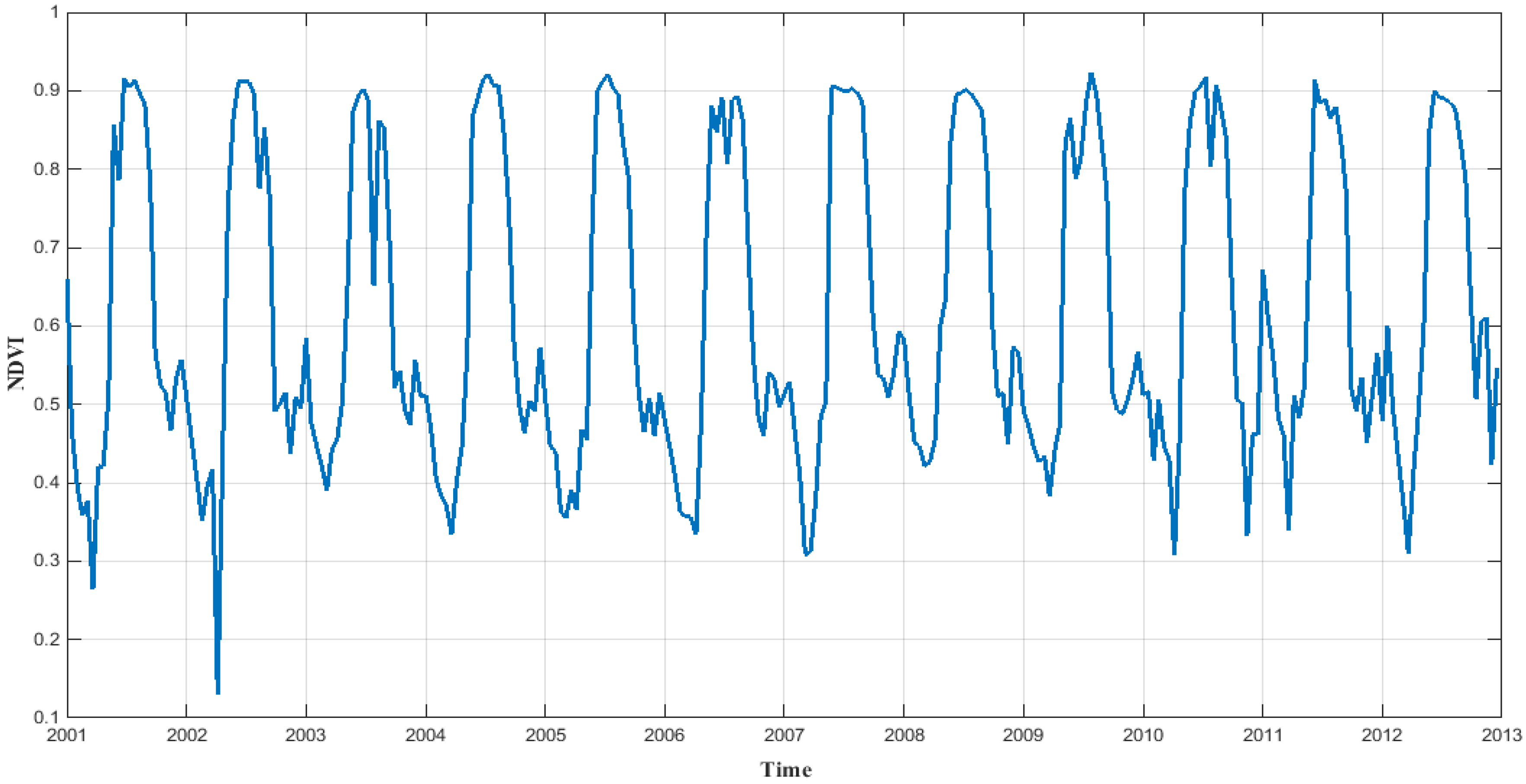
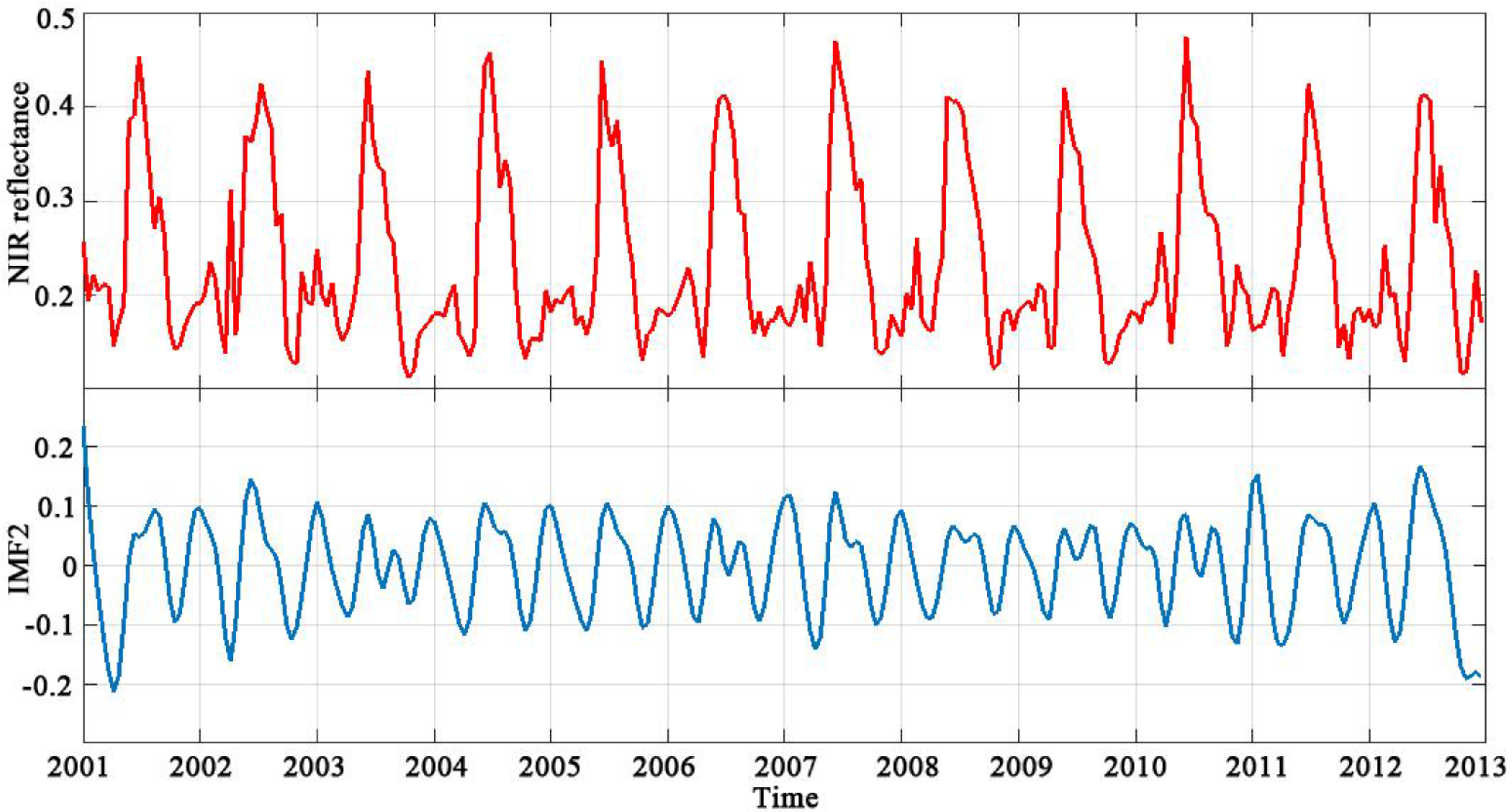
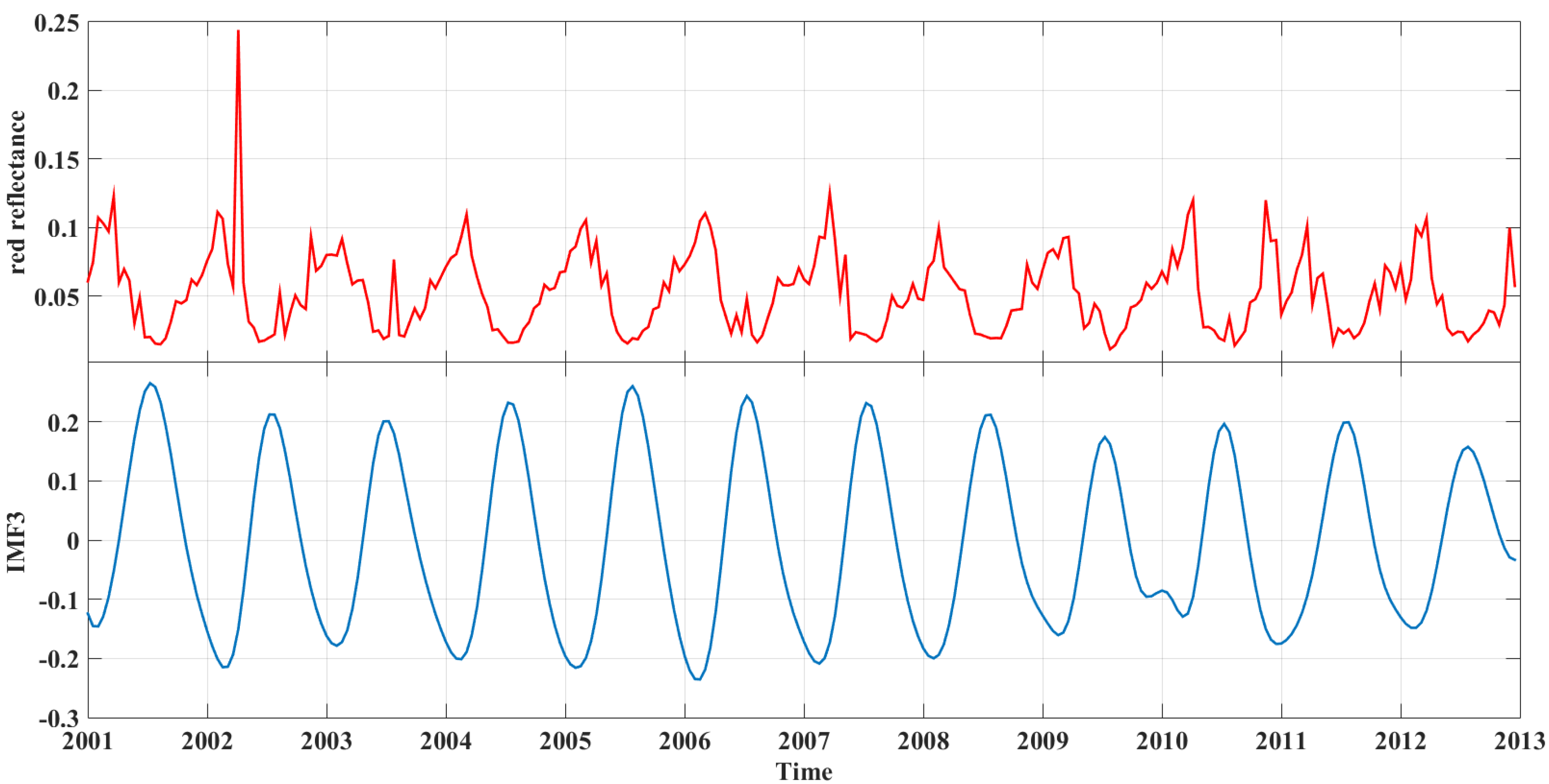
3.1. 16-Day Composite NDVI Time Series of Forest Type

One SITS is generally equivalent to one pixel in a remote sensing image. However, this curve sometimes exhibits particularity for the existing noise. Here, the mean values of 100 SITS in a frame were calculated to obtain a mean time series. Figure 6 illustrates the mean time series of block 1, shown in Figure 5. The EEMD decomposition result of this mean time series is further illustrated in Figure 7, and it was decomposed into seven IMFs and one residue.

Figure 5. False-color-composite image of Landsat TM in the field study region.

Figure 5. False-color-composite image of Landsat TM in the field study region.

Figure 6. Normalized Difference Vegetation Index (NDVI) mean time series.

Figure 6. Normalized Difference Vegetation Index (NDVI) mean time series.

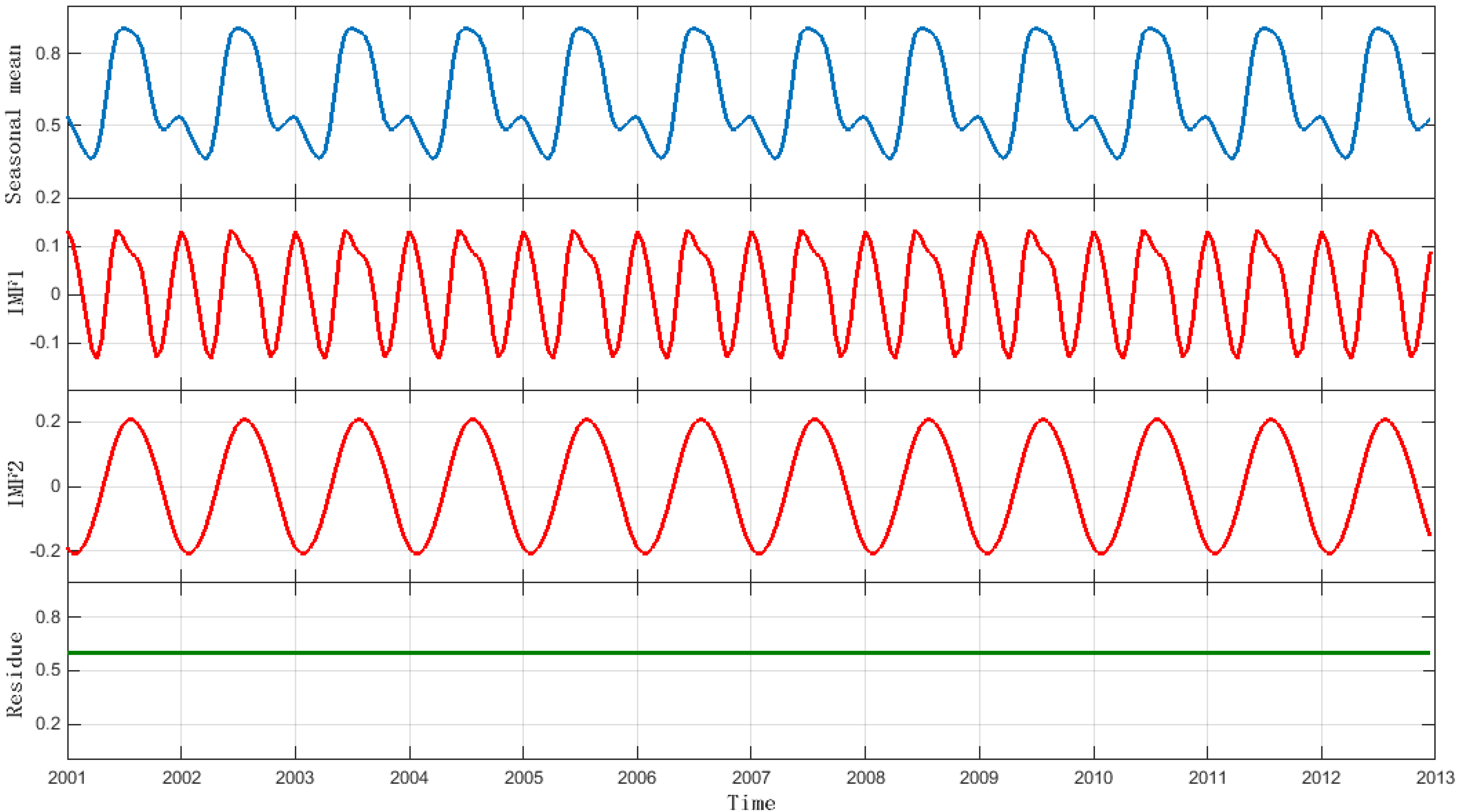
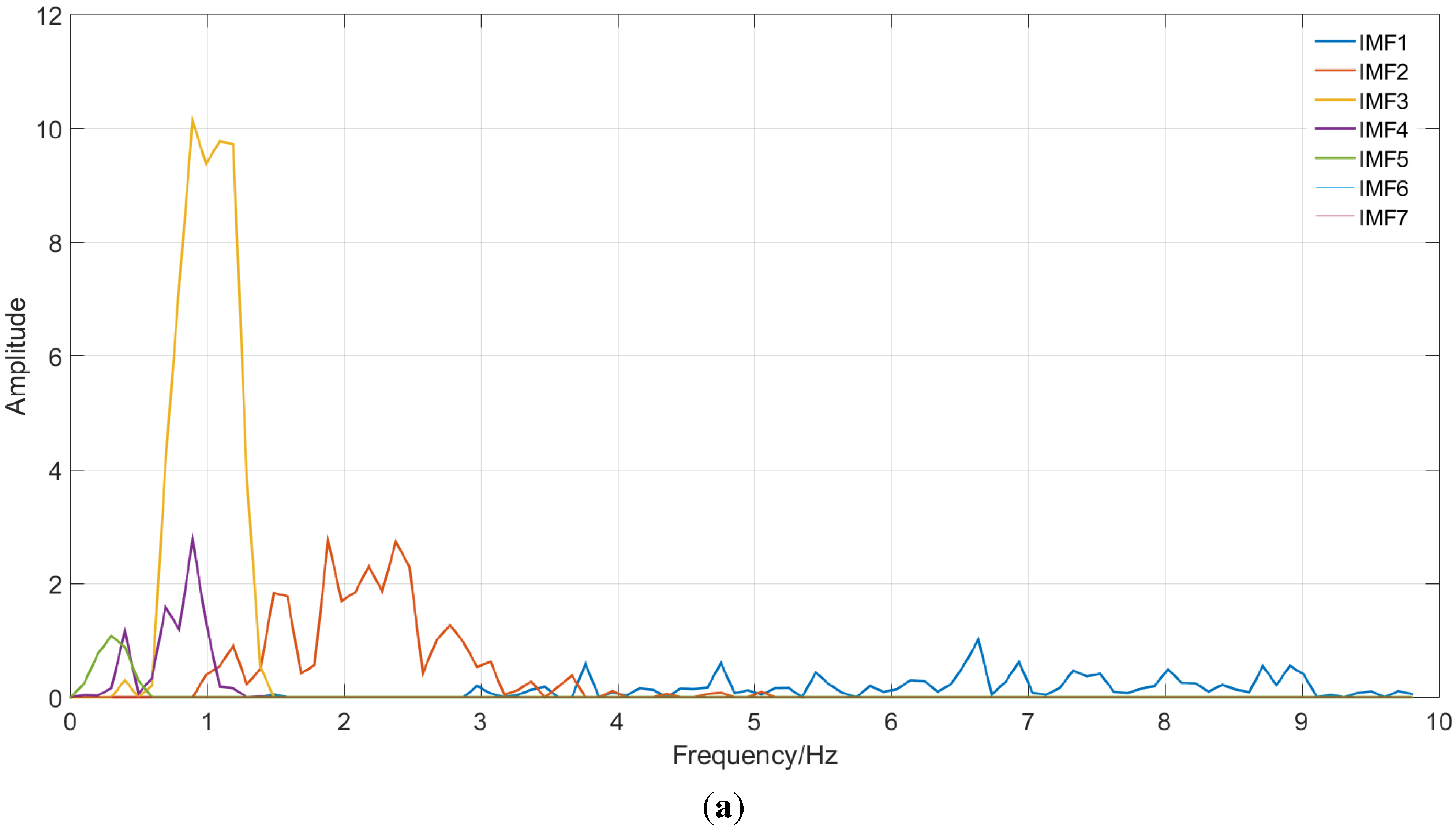
3.1.1. Seasonal-Trend Decomposition

First, the statistical significance test described in Section 2.2 for IMFs is shown in Figure 8. IMF1, which was close to white noise, was subtracted from the original SITS, acquiring one oscillation by averaging the values of a 12-year period. Then, the average seasonal data were obtained by duplicating the oscillation over 12 years, as shown as the blue line in Figure 9. Second, the average seasonal data were decomposed by EEMD and two IMFs were obtained with one-year and half-year oscillations, as illustrated by the red line in Figure 9. From the result, it is apparent that the half-year oscillation is an important component in the seasonal average data. These two IMFs correspond to IMF2 and IMF3, as illustrated in Figure 7. Thus, the seasonal component of this SITS was composed of the original IMF2 and IMF3.

Figure 7. NDVI mean time series decomposed using EEMD. The time series (blue line) is decomposed into 7 IMFs (red line) and a residue (green line).

Figure 7. NDVI mean time series decomposed using EEMD. The time series (blue line) is decomposed into 7 IMFs (red line) and a residue (green line).

Figure 8. Statistical significance test between the energy density and the averaged period. Note that the green dots from left to right indicate the energy density as a function of the averaged period.

Figure 8. Statistical significance test between the energy density and the averaged period. Note that the green dots from left to right indicate the energy density as a function of the averaged period.

To further validate this conclusion, the Hilbert marginal spectrums introduced by Huang et al. [17] were generated for comparison. The comparison is shown in Figure 10. The similarity of the Hilbert marginal spectrums also validated that the two IMFs of the average seasonal data correspond to IMF2 and IMF3 of the original data in frequency.

Figure 9. Average seasonal data decomposed using EEMD.

Figure 9. Average seasonal data decomposed using EEMD.

Figure 10. Comparison of the Hilbert marginal spectra between the real time series and its average seasonal data. (a) Hilbert marginal spectrum of the data shown in Figure 7; (b) Hilbert marginal spectrum of the data shown in Figure 9.

Figure 10. Comparison of the Hilbert marginal spectra between the real time series and its average seasonal data. (a) Hilbert marginal spectrum of the data shown in Figure 7; (b) Hilbert marginal spectrum of the data shown in Figure 9.

As discussed in Section 2.2.2, the trend component with different time scales is generated using the sum of IMFs. This is similar to the traditional seasonal-trend decomposition model of selecting parameters. For this NDVI time series, the trend component was generated by summing IMF5, IMF6, IMF7, and the residue component. The final seasonal-trend composition result is illustrated in Figure 11.

Figure 11. Seasonal-Trend decomposition using EEMD.

Figure 11. Seasonal-Trend decomposition using EEMD.

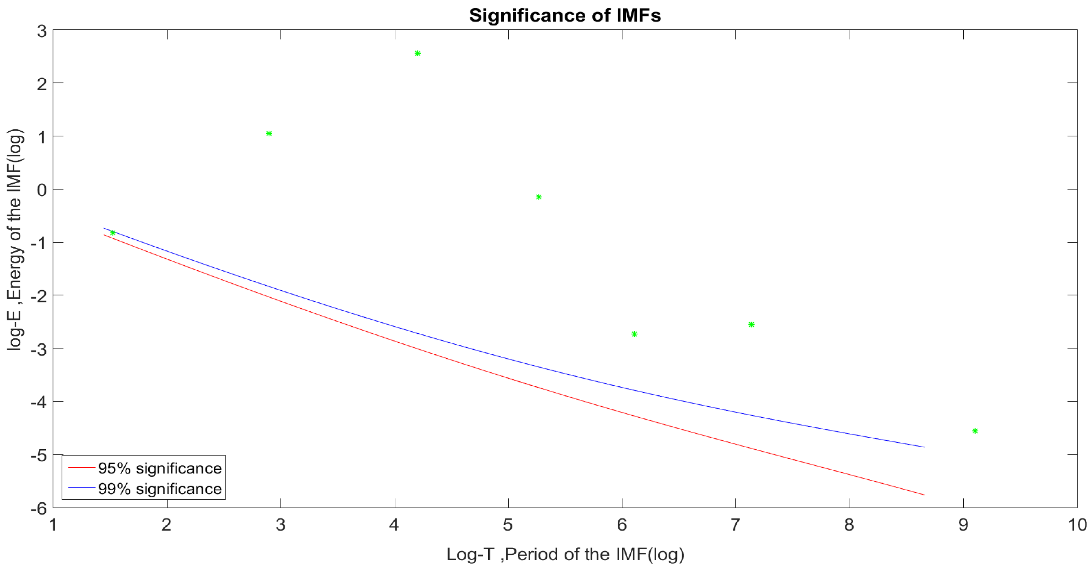
3.1.2. Validation of the Seasonal Component

To validate the effectiveness of the seasonal component, we analyzed the correlation between the biophysical characteristics of vegetation, and IMF2 and IMF3 considering that the NDVI is derived from the red and near-infrared reflectance ratio. From Figure 12 and Figure 13, it is easy to observe that the oscillation of the spectral reflectance time series of near-infrared and red are closely related to IMF2 and IMF3, which were obtained by decomposing the NDVI time series. It was noted that the spectral reflectance time series of the near infrared (red) bands had similar wave characteristics. In particular, the half-annual wave of IMF2 was incurred by the half-annual wave of the near infrared band reflectance, whereas the annual wave of IMF3 was the joint result of the near infrared and red bands.

As the red line shown in Figure 12 illustrates, there were two peaks in a year in the spectral reflectance time series of the near-infrared band. One was in the summer due to the high reflection of vegetation, and the other was in the winter due to the high reflection of soil and snow. Comparing the curves of the spectral reflectance time series of the near-infrared band and IMF2 (blue line), the oscillations of these two series are more or less consistent, as shown in Figure 12. Additionally, as illustrated in Figure 13, there is only one peak in the spectral reflectance time series of the red band in a year. The valley was in the summer due to the strong absorption of the vegetation. The oscillations of IMF3 were similar to those of the red band, and both of them had one regular cycle per year. The peaks and valleys were reversed between the two time series because the red band reflectance is the subtraction of the vegetation indices.

It should be noted that, by definition, the mean value of the upper and lower envelopes of an IMF is zero. However, it is almost impossible for the spectral reflectance time series to have a mean of zero. Hence, the IMF is a frequency component of the original time series, and can be related only to the frequency of the spectral reflectance, but hardly reflect the information of the amplitude or phase.

Figure 12. Spectral reflectance time series of near-infrared band and IMF2.

Figure 12. Spectral reflectance time series of near-infrared band and IMF2.

Figure 13. Spectral reflectance time series of red band and IMF3.

Figure 13. Spectral reflectance time series of red band and IMF3.

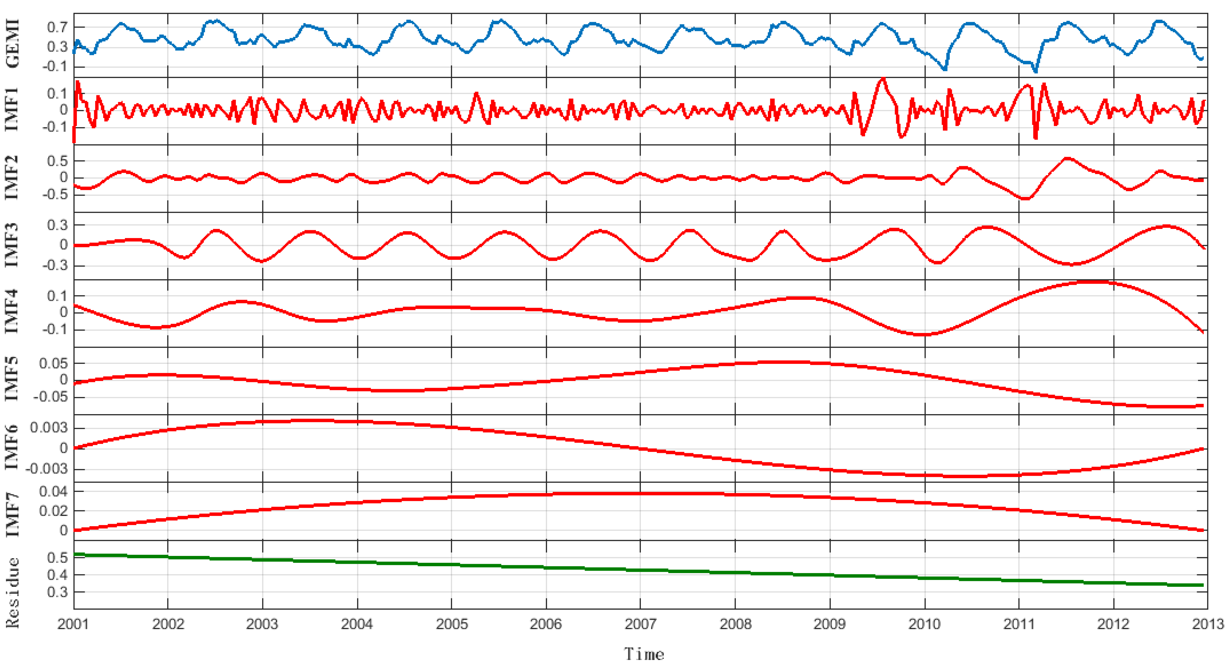
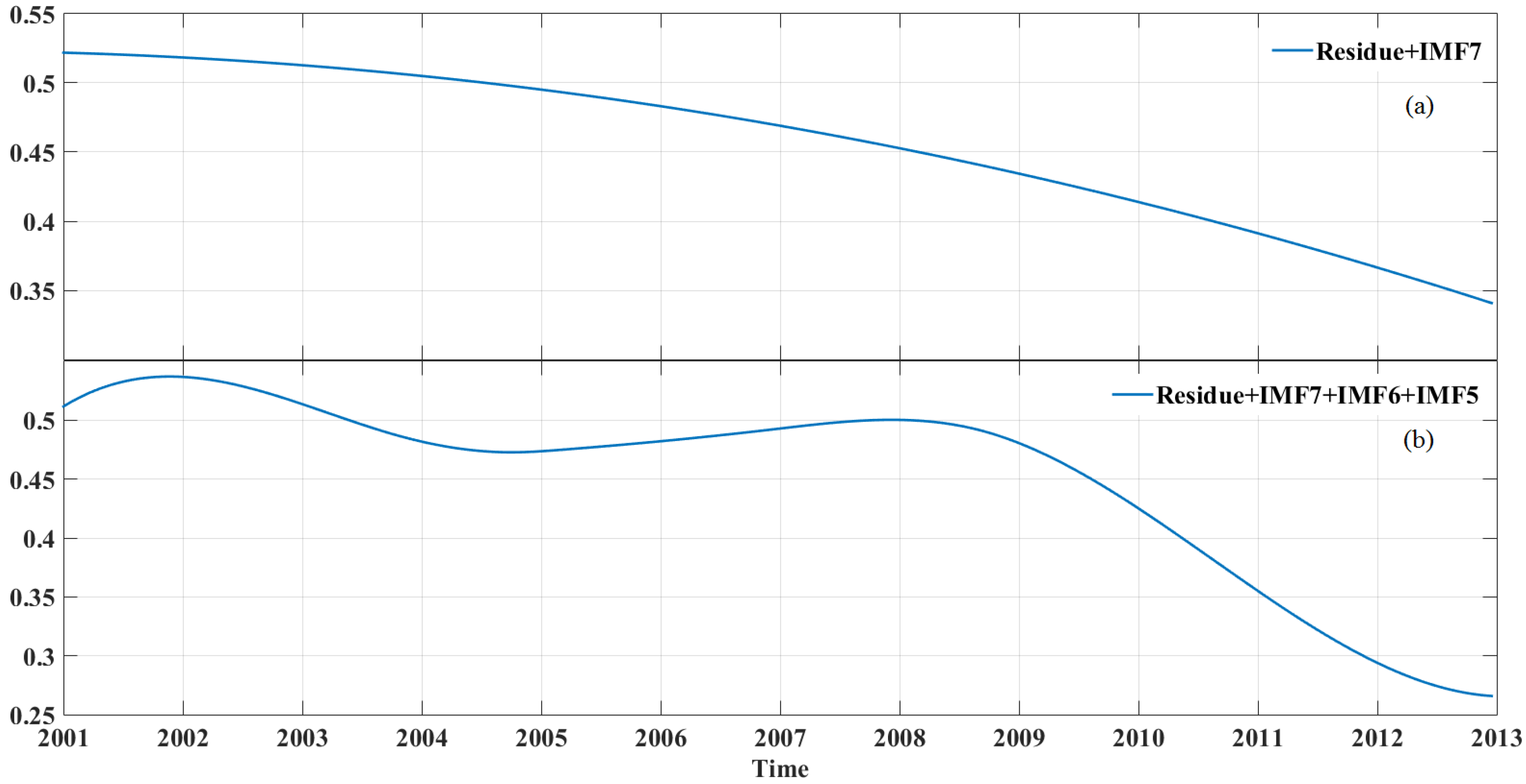
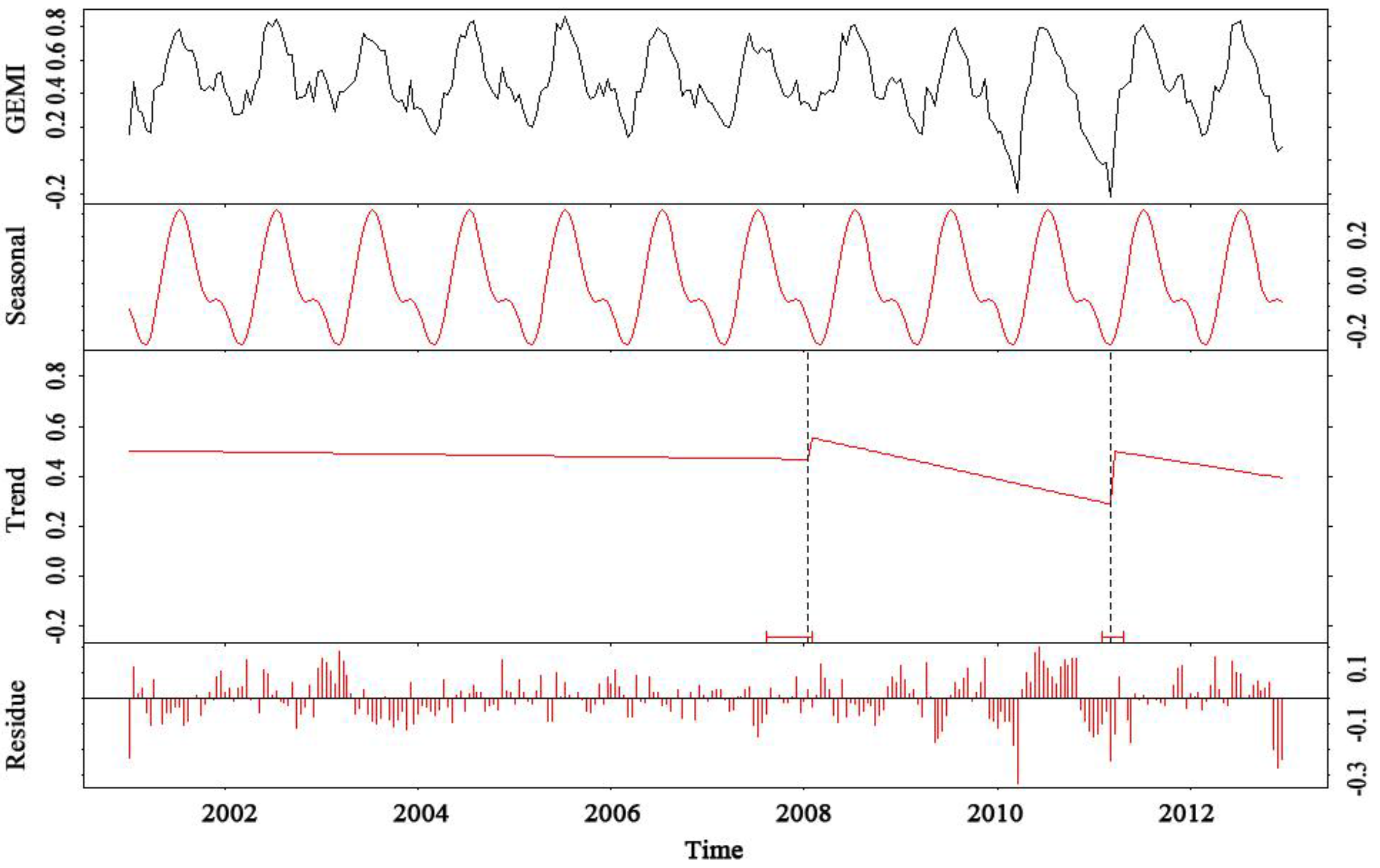
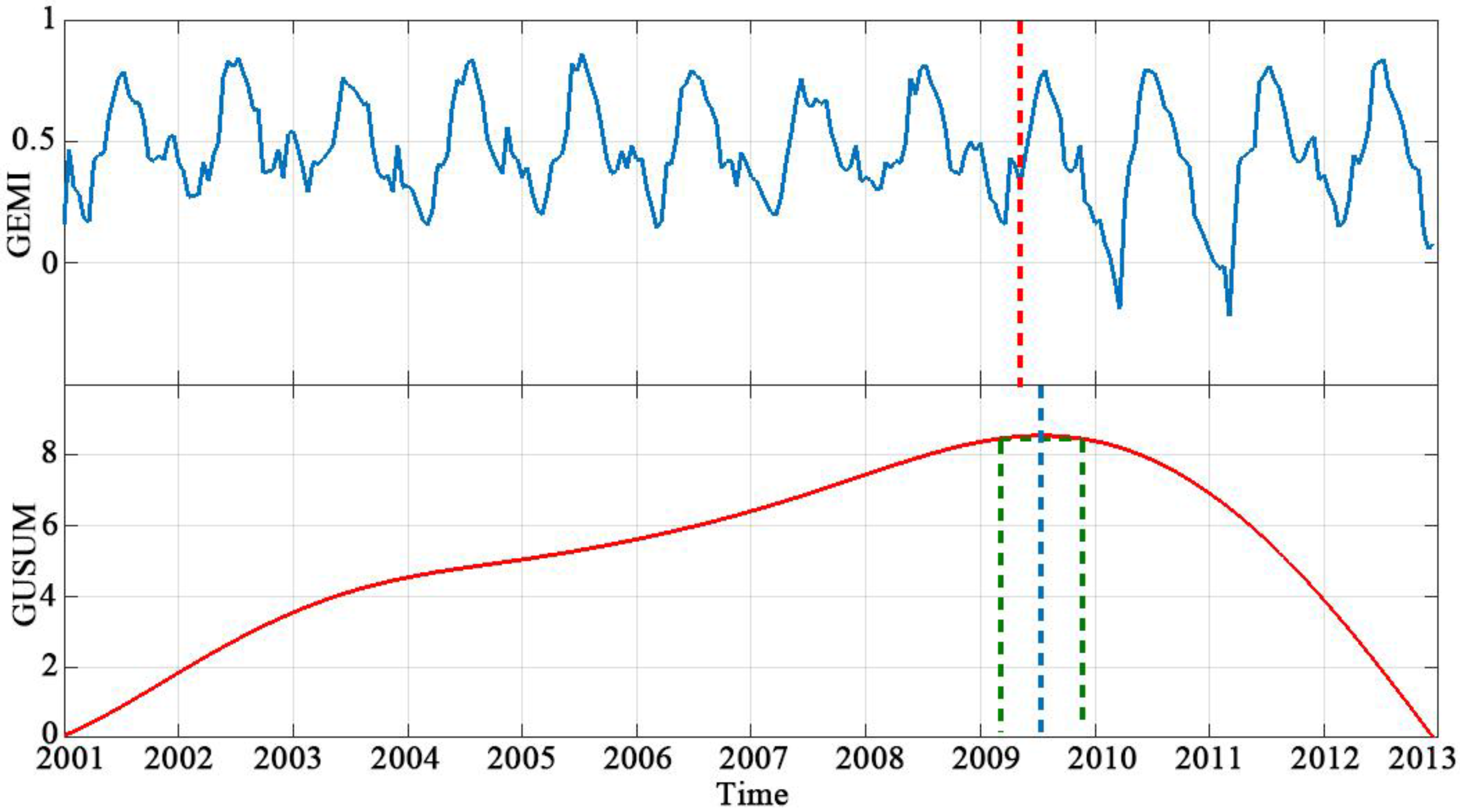
3.2. Sixteen-Day Composition GEMI Time Series with Disturbance

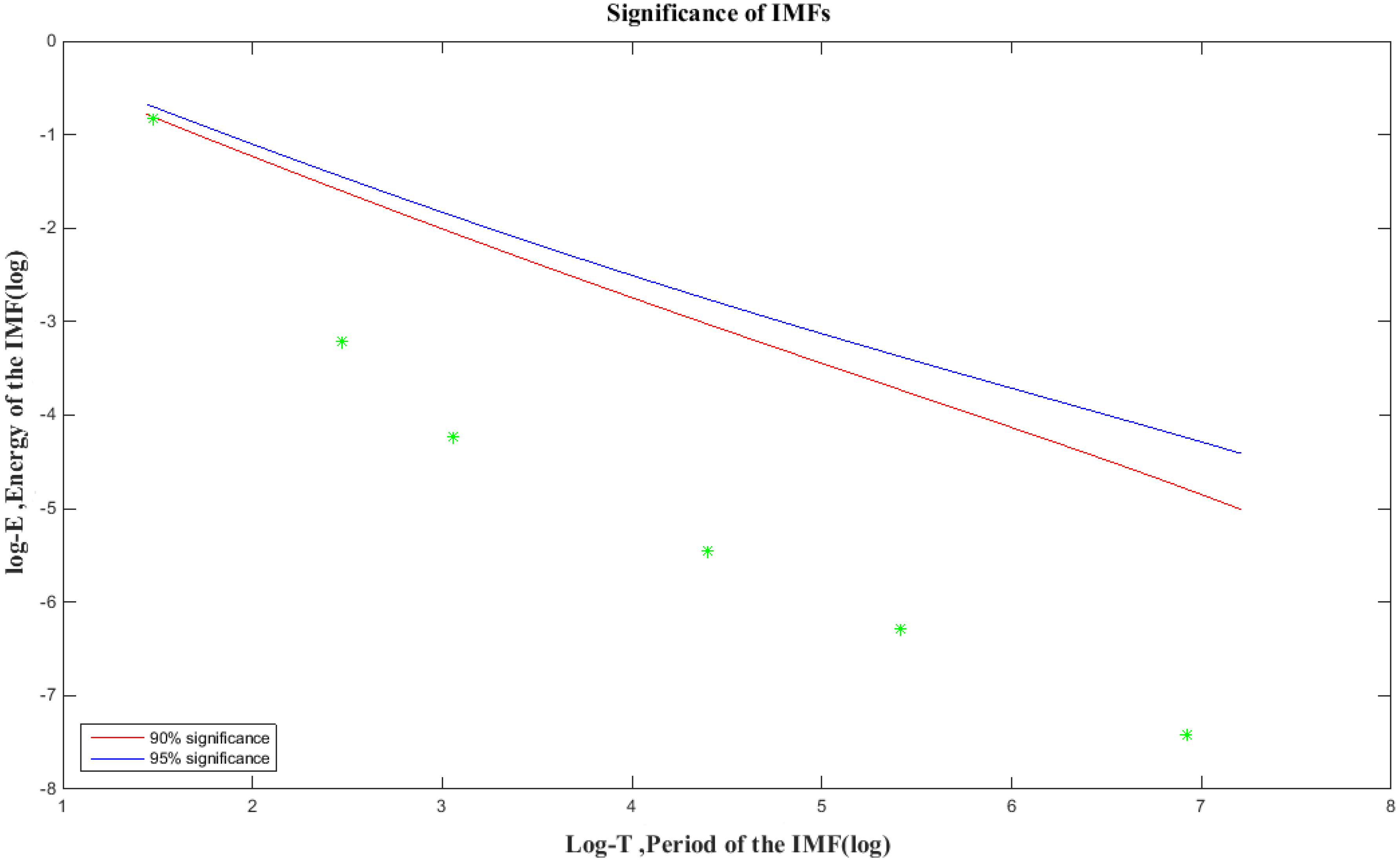
In this experiment, we further examined the application of the trend component in disturbance information detection. A 16-day GEMI time series of block 2 as shown in Figure 14 (blue line), was employed. A bushfire led to vegetation deterioration and a slump in biomass. A slump also occurred in the time series in the vegetation index. These changes were usually structural changes. It was difficult to directly determine the disturbance in the 16-day GEMI time series. EEMD was applied to decompose the SITS. The red lines show the IMFs from high to low frequencies, respectively, which are illustrated in Figure 14, and the green line indicates the residue.

Figure 14. Global Environment Monitoring Index (GEMI) time series decomposed using EEMD.

Figure 14. Global Environment Monitoring Index (GEMI) time series decomposed using EEMD.

Once the effects of seasonal variation and high-frequency information (as noise) were removed, the observation of a large variation scale in structural changes compared to that in the moderate yearly variations was expected. These changes were also holistic changes and reflected in the IMFs with the lowest frequency and the residue. Figure 15a illustrates the trend component formulated using residue and the IMF7 decomposed from the GEMI time series using EEMD. Despite the descending tendency in the trend component, it was difficult to accurately locate the change point. We performed change point detection on the trend component using the cumulative sum (CUSUM) algorithm [30,31]; the detected change point had an obvious deviation from the actual time a drastic change occurred. As illustrated in Figure 16a, the detected change point represented by the red dashed line corresponded to scene 18 of year 2007 (30 September–15 October), whereas the actual occurrence of the fire was scene 8 of year 2009 (21 April–7 May).

Figure 15. (a,b) Trend components with different time scales of the GEMI time series.

Figure 15. (a,b) Trend components with different time scales of the GEMI time series.

Hence, more high frequency IMFs need to be added to the trend component to obtain a more precise position of the change point. Based on the analysis in Section 2.2.3, an energy ratio of the IMF and the residue less than one should be used to avoid a false change point. The ratio of the threshold should be selected depending on the intensity of the change. The more intense change that occurs, the less influence it has on the change detection by high-frequency IMFs, and a wider range of threshold could be chosen. A large number of experiments showed that, in this case, a threshold value between 0.4 and 0.8 was recommended. In this work, we set the ratio of the threshold to the residue as 0.5, and IMF7, IMF6, and IMF5 should be added to the residue to form the trend component according to their energy values shown in Table 1. The final trend component is illustrated in Figure 15b, where it can be clearly observed that the structural variation appeared after the year 2009. We then performed change point detection on the trend component using the CUSUM algorithm. The detected discontinuity represented by the red dashed line corresponds to scene 13 of year 2009 (12–27 July), as in Figure 16b. The change point in Figure 16a is obviously more precise; where the position of the change point is closer to the real change point.

Figure 16. (a,b) The results of change point detection of different trend components.

Figure 16. (a,b) The results of change point detection of different trend components.

Table 1. Energy of the residue and IMFs illustrated in Figure 14.

	IMF1	IMF2	IMF3	IMF4	IMF5	IMF6	IMF7	Residue
Energy	0.878	2.606	6.860	1.522	0.370	0.002	0.212	0.760

Table 1. Energy of the residue and IMFs illustrated in Figure 14.

	IMF1	IMF2	IMF3	IMF4	IMF5	IMF6	IMF7	Residue
Energy	0.878	2.606	6.860	1.522	0.370	0.002	0.212	0.760

The Breaks for Additive Season and Trend (BFAST) method [32,33,34] may also be used to detect the precise change point, although it needs proper parameters. Otherwise, a false change point would be found. For example, two false change points were detected in the same SITS, as illustrated in Figure 17.

Figure 17. The results of change point detection of Breaks for Additive Season and Trend (BFAST) algorithm.

Figure 17. The results of change point detection of Breaks for Additive Season and Trend (BFAST) algorithm.

For the time scale of the trend component, there is an offset between the detected change point and the actual point. Thus, the change point is sometimes substituted by the change range, and we assess the precise point in the change range. Figure 18 further illustrates the detection results. The detected change point was represented by the blue dashed line, and the change range is represented by the green dashed line with the threshold of 0.1. The actual occurrence of the fire is represented by the red dashed line.

Figure 18. The results of change point detection and change range detection.

Figure 18. The results of change point detection and change range detection.

Disturbances usually cause abrupt changes in time. In this instance, the value should be lower than the values in the previous and next years. Furthermore, vegetation recovery is a gradual process. Hence, compared with the adjacent years, the lowest values should last for a period. According to this phenomenon, Figure 19 further illustrates the comparison between the adjacent years during the interval between the green lines in Figure 18. The lowest values start from the 8th point in 2009, and last for a period. Therefore, the change position can be updated to the 8th point (23 April to 8 May) in 2009.

Figure 19. Comparison with adjacent years.

Figure 19. Comparison with adjacent years.

Finally, the overall process described was applied to the MODIS data pixel by pixel, as shown in Figure 20. A burned area was detected, as illustrated in Figure 20b. The red area represents the burned area, and the green indicates unburned area. A Landsat TM image shot in 23 May 2009 was used as a reference map in Figure 20a. Compared to the reference map, the detection results clearly show the efficiency of the proposed method.

Figure 20. Detection map of the proposed method. (a) Landsat TM image shot on 23 May 2009. (b) Burned area detection map.

Figure 20. Detection map of the proposed method. (a) Landsat TM image shot on 23 May 2009. (b) Burned area detection map.

4. Conclusions

We presented a decomposition approach for SITS based on EEMD. The proposed method first decomposed time series into several IMFs and a residue, and then chose appropriate IMFs to make up the seasonal component according to the spectral characteristics of the targets and the trend component according to the time scale. From experimental analysis, the proposed decomposition approach was proven to be simple and flexible for the construction of seasonal and trend components according to the applications. It provided robust trend and seasonal components that were not distorted by transient, aberrant behavior. It should be noted that the method is easy for computer implementation and can quickly finish computation, even for long time series, which fulfills the criteria of the seasonal-trend decomposition model proposed by Cleveland et al. [10]. In addition, the seasonal and trend components from this decomposition were intrinsic with clear meanings. Furthermore, the decomposition with the basis function was derived from the data by EEMD sifting procedures, instead of a priori functional basis, and the procedure was truly adaptive.

Based on the investigation of this work, the considerations for further research fall into two main categories:

(1)

Further algorithm improvement should consider the sensitivity of change point detection of the seasonal or trending component.

(2)

Further research is necessary to incrementally update an event database when new observations are available and to enhance the prediction algorithm to achieve real-time change detection (see Schnebele, et al. [35]).

References

1. Petitjean, F.; Inglada, J.; Gançarski, P. Satellite image time series analysis under time warping. IEEE Trans. Geosci. Remote Sens. 2012, 50, 3081–3095. [Google Scholar] [CrossRef]
2. Bowerman, B.L.; O’Connell, R.T.; Koehler, A.B. Forecasting, Time Series, and Regression: An Applied Approach, 4th ed.; South-Western College Pub: Cincinnati, OH, USA, 2004. [Google Scholar]
3. Liu, K.; Du, Q.; Yang, H.; Ma, B. Optical flow and principal component analysis-based motion detection in outdoor videos. EURASIP J. Adv. Signal Process. 2010. [Google Scholar] [CrossRef]
4. Kandasamy, S.; Baret, F.; Verger, A.; Neveux, P.; Weiss, M. A comparison of methods for smoothing and gap filling time series of remote sensing observations—Application to MODIS LAI products. Biogeosciences 2013, 10, 4055–4071. [Google Scholar] [CrossRef]
5. Jönsson, P.; Eklundh, L. Seasonality extraction by function fitting to time-series of satellite sensor data. IEEE Trans. Geosci. Remote Sens. 2002, 40, 1824–1832. [Google Scholar] [CrossRef]
6. Zhang, X.; Friedl, M.A.; Schaaf, C.B.; Strahler, A.H.; Schneider, A. The footprint of urban climates on vegetation phenology. Geophys. Res. Lett. 2004, 31. [Google Scholar] [CrossRef]
7. De Beurs, K.M.; Henebry, G.M. A statistical framework for the analysis of long image time series. Int. J. Remote Sens. 2005, 26, 1551–1573. [Google Scholar] [CrossRef]
8. Eastman, J.R.; Sangermano, F.; Ghimire, B.; Zhu, H.; Chen, H.; Neeti, N.; Cai, Y.; Machado, E.A.; Crema, S.C. Seasonal trend analysis of image time series. Int. J. Remote Sens. 2009, 30, 2721–2726. [Google Scholar] [CrossRef]
9. Parmentier, B.; Eastman, J.R. Land transitions from multivariate time series: Using seasonal trend analysis and segmentation to detect land-cover changes. Int. J. Remote Sens. 2014, 35, 671–692. [Google Scholar] [CrossRef]
10. Cleveland, R.B.; Cleveland, W.S.; McRae, J.E.; Terpenning, I. STL: A seasonal-trend decomposition procedure based on LOESS. J. Off. Stat. 1990, 6, 3–73. [Google Scholar]
11. Vautard, R.; Yiou, P.; Ghil, M. Singular-spectrum analysis: A toolkit for short, noisy chaotic signals. Phys. D Nonlinear Phenom. 1992, 58, 95–126. [Google Scholar] [CrossRef]
12. Mahecha, M.D.; Fürst, L.M.; Gobron, N.; Lange, H. Identifying multiple spatiotemporal patterns: A refined view on terrestrial photosynthetic activity. Pattern Recognit. Lett. 2010, 31, 2309–2317. [Google Scholar] [CrossRef]
13. Forkel, M.; Carvalhais, N.; Verbesselt, J.; Mahecha, M.D.; Neigh, C.S.; Reichstein, M. Trend change detection in NDVI time series: Effects of inter-annual variability and methodology. Remote Sens. 2013, 5, 2113–2144. [Google Scholar] [CrossRef]
14. Wu, Z.; Huang, N.E. Ensemble empirical mode decomposition: A noise-assisted data analysis method. Adv. Adapt. Data Anal. 2009, 1, 1–41. [Google Scholar] [CrossRef]
15. Tucker, C.J. Red and photographic infrared linear combinations for monitoring vegetation. Remote Sens. Environ. 1979, 8, 127–150. [Google Scholar] [CrossRef]
16. Pinty, B.; Verstraete, M.M. GEMI: A non-linear index to monitor global vegetation from satellites. Vegetatio 1992, 101, 15–20. [Google Scholar] [CrossRef]
17. Huang, N.E.; Shen, Z.; Long, S.R.; Wu, M.C.; Shih, H.H.; Zheng, Q.; Yen, N.-C.; Tung, C.C.; Liu, H.H. The empirical mode decomposition and the hilbert spectrum for nonlinear and non-stationary time series analysis. Proc. R. Soc. Lond. A 1998, 454, 903–995. [Google Scholar] [CrossRef]
18. Gloersen, P.; Huang, N. Comparison of interannual intrinsic modes in hemispheric sea ice covers and other geophysical parameters. IEEE Trans. Geosci. Remote Sens. 2003, 41, 1062–1074. [Google Scholar] [CrossRef]
19. Huang, N.E.; Shen, S.S. Hilbert-Huang Transform and Its Applications; World Scientific: Singapore, 2005; Volume 5. [Google Scholar]
20. Kaplan, N.; Erer, I. An additive empirical mode decomposition based method for the fusion of remote sensing images. In Proceedings of the 6th International Conference on Recent Advances in Space Technologies (RAST), Istanbul, Turkey, 12–14 June 2013; pp. 165–169.
21. Wang, T.; Zhang, M.; Yu, Q.; Zhang, H. Comparing the applications of emd and eemd on time-frequency analysis of seismic signal. J. Appl. Geophys. 2012, 83, 29–34. [Google Scholar] [CrossRef]
22. Xu, M.; Shang, P.; Lin, A. Cross-correlation analysis of stock markets using EMD and EEMD. Phys. A Stat. Mech. Appl. 2016, 442, 82–90. [Google Scholar] [CrossRef]
23. Lei, Y.; He, Z.; Zi, Y. Application of the EEMD method to rotor fault diagnosis of rotating machinery. Mech. Syst. Signal Process. 2009, 23, 1327–1338. [Google Scholar] [CrossRef]
24. Goel, G.; Hatzinakos, D. Ensemble empirical mode decomposition for time series prediction in wireless sensor networks. In Proceedings of the International Conference on Computing, Networking and Communications (ICNC), Honolulu, HI, USA, 3–6 February 2014; pp. 594–598.
25. Ren, H.; Wang, Y.-L.; Huang, M.-Y.; Chang, Y.-L.; Kao, H.-M. Ensemble empirical mode decomposition parameters optimization for spectral distance measurement in hyperspectral remote sensing data. Remote Sens. 2014, 6, 2069–2083. [Google Scholar] [CrossRef]
26. De Ridder, S.; Neyt, X.; Pattyn, N.; Migeotte, P.-F. Comparison between eemd, wavelet and fir denoising: Influence on event detection in impedance cardiography. In Proceedings of the Annual International Conference of the IEEE Engineering in Medicine and Biology Society, Boston, MA, USA, 30 August–3 September 2011; pp. 806–809.
27. Wu, Z.; Huang, N.E.; Long, S.R.; Peng, C.-K. On the trend, detrending, and variability of nonlinear and nonstationary time series. Proc. Natl. Acad. Sci. USA 2007, 104, 14889–14894. [Google Scholar] [CrossRef] [PubMed]
28. Wu, Z.; Huang, N.E. A study of the characteristics of white noise using the empirical mode decomposition method. Proc. R. Soc. Lond. A 2004, 460, 1597–1611. [Google Scholar] [CrossRef]
29. Moghtaderi, A.; Flandrin, P.; Borgnat, P. Trend filtering via empirical mode decompositions. Comput. Stat. Data Anal. 2013, 58, 114–126. [Google Scholar] [CrossRef]
30. Kučera, J.; Barbosa, P.; Strobl, P. Cumulative sum charts-a novel technique for processing daily time series of MODIS data for burnt area mapping in Portugal. In Proceedings of the International Workshop on the Analysis of Multi-temporal Remote Sensing Images, Leuven, Belgium, 18–20 July 2007; pp. 1–6.
31. Grobler, T.L.; Ackermann, E.R.; van Zyl, A.J.; Olivier, J.C.; Kleynhans, W.; Salmon, B.P. Using page’s cumulative sum test on MODIS time series to detect land-cover changes. IEEE Geosci. Remote Sens. Lett. 2013, 10, 332–336. [Google Scholar] [CrossRef]
32. Verbesselt, J.; Hyndman, R.; Newnham, G.; Culvenor, D. Detecting trend and seasonal changes in satellite image time series. Remote Sens. Environ. 2010, 114, 106–115. [Google Scholar] [CrossRef]
33. Verbesselt, J.; Hyndman, R.; Zeileis, A.; Culvenor, D. Phenological change detection while accounting for abrupt and gradual trends in satellite image time series. Remote Sens. Environ. 2010, 114, 2970–2980. [Google Scholar] [CrossRef]
34. Verbesselt, J.; Zeileis, A.; Herold, M. Near real-time disturbance detection using satellite image time series. Remote Sens. Environ. 2012, 123, 98–108. [Google Scholar] [CrossRef]
35. Schnebele, E.; Cervone, G.; Kumar, S.; Waters, N. Real time estimation of the calgary floods using limited remote sensing data. Water 2014, 6, 381–398. [Google Scholar] [CrossRef]