Article

The Utility of AISA Eagle Hyperspectral Data and Random Forest Classifier for Flower Mapping

1
International Center for Insect Physiology and Ecology (ICIPE), P.O. Box 30772, Nairobi 00100, Kenya
2
Department of Agronomy, Faculty of Agriculture, University of Khartoum, Khartoum North 13314, Sudan
3
Department of Geosciences and Geography, University of Helsinki, Gustaf Hällströmin katu 2b, Helsinki 00560, Finland
4
Department of Geography, School of Agricultural, Environment and Earth Sciences, University of KwaZulu-Natal, Pietermaritzburg 3209, South Africa
*
Author to whom correspondence should be addressed.
Remote Sens. 2015, 7(10), 13298-13318; https://doi.org/10.3390/rs71013298
Submission received: 5 August 2015 / Revised: 18 September 2015 / Accepted: 25 September 2015 / Published: 12 October 2015

Abstract

:
Knowledge of the floral cycle and the spatial distribution and abundance of flowering plants is important for bee health studies to understand the relationship between landscape and bee hive productivity and honey flow. The key objective of this study was to show how AISA Eagle hyperspectral data and random forest (RF) can be optimally utilized to produce flowering and spatially explicit land use/land cover (LULC) maps for a study site in Kenya. AISA Eagle imagery was captured at the early flowering period (January 2014) and at the peak flowering season (February 2013). Data on white and yellow flowering trees as well as LULC classes in the study area were collected and used as ground-truth points. We utilized all 64 AISA Eagle bands and also used variable importance in RF to identify the most important bands in both AISA Eagle data sets. The results showed that flowering was most accurately mapped using the AISA Eagle data from the peak flowering period (85.71%–88.15% overall accuracy for the peak flowering season imagery versus 80.82%–83.67% for the early flowering season). The variable optimization (i.e., variable selection) analysis showed that less than half of the AISA bands (n = 26 for the February 2013 data and n = 21 for the January 2014 data) were important to attain relatively reliable classification accuracies. Our study is an important first step towards the development of operational flower mapping routines and for understanding the relationship between flowering and bees’ foraging behavior.

Graphical Abstract

1. Introduction

In recent years, concerns about bee health and hive productivity have been the focus of numerous studies and intervention projects worldwide (e.g., [1,2]). Specifically, attention has been paid to factors that threaten honeybee health such as parasites, pathogens, abiotic stress factors, and land use and land cover (LULC) changes that often lead to a decrease in flowering plants within the landscape matrix. Essentially, the quality and quantity of honey and honey products is reliant on the availability of flowering melliferous plants (as pollen and nectar sources) in the landscape [3]. Honeybee products including honey, wax, propolis, and royal jelly can be sold by rural communities to generate income [3,4]. Knowledge on the density and diversity of melliferous plants as well as floral cycle and intensity is important for an optimal placement of bee hives within the landscape matrix and moreover to understand honeybee foraging behavior and hive productivity in terms of honey quantity and quality [3,4].
However, data sets on the spatio-temporal distribution of flowering plants are largely not available for phenological and ecological response studies. Furthermore, the relationship between flowering response in the landscape and hive production is largely unknown [5]. The spatio-temporal floral coverage within a landscape mosaic depends mainly on local environmental factors [6,7], landscape fragmentation and land form. Regular field investigations to better understand spatio-temporal floral patterns are costly, time-consuming, tedious, and relatively inaccurate especially if performed by various field observers. Rapid, reliable, accurate, and synoptic techniques are therefore required for mapping and monitoring flowering intensity and floral cycles to guide bee keeping activities. A spatial flowering data set can, for instance, be used by bee keepers as a decision aid as to where in the landscape apiaries should be most optimally set up in order to minimize foraging distances and increase hive productivity. Explicit LULC data in conjunction with flowering information provides a more comprehensive and useful overview of the landscape matrix as an important bee foraging space as certain LULC classes could be habitats for flowering plants.
Recently, remotely sensed data sets have been used successfully to provide accurate and fine scale estimates of flower coverage [5,8]. Chen et al. [4] utilized in situ hyperspectral measurements to calculate a flower index that accurately estimated flower coverage in a grassland biome in central Asia. Hyperspectral data offer dozens to hundreds of narrow and contiguous spectral measurements in the visible (400–700 nm), near infrared (700–1300 nm), and often in the shortwave near infrared (SWIR:1300–2500 nm) regions of the electromagnetic spectrum [9,10] that allow the depiction of subtle spectral features often within complex landscapes such as semi-arid savannas [11,12]. Though the study of Chen et al. [4] has made a significant contribution concerning flower coverage estimations, their study only focused on one flowering species and, since they used in situ hyperspectral data, only a localized (smaller) area could be assessed. Landmann et al. [8] used spectral linear unmixing and change vector analysis on AISA Eagle hyperspectral data for mapping the abundance, distribution, and floral cycle of melliferous plants. A short-term floral cycle map was successfully produced with an overall accuracy between 80.7% and 83%. However, the investigation of Landmann et al. [8] did not consider species-specific flowering colors in the linear unmixing-based mapping approach. Color of flowers could be an important measure of bees foraging preference [13,14]. More studies that test the utility of hyperspectral data to map melliferous plants that exhibit different flowering colors are required.
Taking advantage of the rich spectral information, various types of nonparametric machine learning classification methods have been applied to analyze hyperspectral data. For instance, random forest, support vector machines and neural network were employed in numerous hyperspectral studies to discriminate vegetation communities [15], genera [16], and plant species (e.g., [17,18,19]). However, the high dimensionality in hyperspectral data is often problematic when the number of field samples is smaller than the number of spectral features [20]. In addition, the dimensionality of hyperspectral features might not be captured in a linear projection. Therefore, non-linear classification methods such as random forest, that produce variable selection as a by-product during the learning process, are considered efficient algorithms for the analyses of hyperspectral data especially in biomes where spectral mixing is highly non-linear (e.g., [21,22,23,24,25,26]).
We mapped flowering plants in a key bee keeping area in Kenya using airborne AISA Eagle hyperspectral data and optimized RF for the two different image acquisition dates; i.e., at the maximum period of flowering in February 2013 and at the beginning of flowering period in January 2014. Specifically, we aimed to show how RF can be optimized, using grid search and variable selection, to produce maps of flowering plants and other LULC classes in a highly complex, dynamic, and semi-arid agro-ecological landscape in Kenya. We applied our classification approach to two different time points to evaluate the repeatability of our methods and test whether the approach could be transferable to different floral periods (i.e., beginning of flowering and peak flowering periods). Flowering maps for the two time periods are useful information feeds that will help to understand how floral change (i.e., phenology) affects honeybee behavior, honey flow, and hive productivity.

2. Experimental Section

2.1. Study Area

The study site covers about 3 km2 and is located about 17 km north of Mwingi town in the Kitui County of Kenya (0.770°S and 38.143°E, 933m above sea level) (Figure 1). Mwingi is a semi-arid area with two rainy seasons that peak in April (147 mm mean annual precipitation in a normal period) and in November (270 mm mean annual precipitation in a normal period) [8]. The temperature ranges are between 15 °C and 30 °C, and the hottest periods are between February and March and September to October, while the coldest months are July and August [27]. The main melliferous plants are Acacia spp., Terminalia brownie, Aspilia mozambensis, Cassia diambotia, Cassia semea, Euphobia spp., Solonium incunum, Boscia, and Grewia spp. Most of these plants produce white and yellow flowers between January and May [28], with a few plants species flowering in December.
The study area is mainly an agro-ecological mosaic with the main crops being maize (Zea mays) and sorghum (Sorghum bicolor). Farmers employ traditional systems for crop production like contour farming and clearing and burning of shrubs and trees. Therefore, few patches of natural vegetation are left that could be used by bees for foraging and nesting [29,30]. The area is one of the most important beekeeping areas in Kenya with over 2.000 farmers practicing bee farming [31,32]. However, a decrease in colony sizes could be observed in recent years mainly due to droughts and changes in temperature regimes [31].
Figure 1. Location of the study area in Mwingi Central Division, Kitui County, Kenya and field sample locations overlaid on a true-color AISA Eagle image captured in February 2013. Image extent refers to the full extent of AISA Eagle image.
Remotesensing 07 13298 g001

2.2. Image Acquisition and Pre-Processing

Hyperspectral data were captured using the AISA Eagle imaging spectrometer at a flight altitude of 860 m during the maximum flowering period on the 14 February 2013 and at the beginning of floral period on the 11 January 2014. AISA Eagle is an airborne-based sensor with a pushbroom scanner and instantaneous field of view (IFOV) of 0.648 MRad, field of view (FOV) of 36.04°, 969 pixels across the spatial axis and a pixel size of 0.6 m. The sensor was used in eight times spectral binning mode, which produces output images in 64 bands with a full width at half maximum (FWHM) of 8–10.5 nm in the spectral range 400–1000 nm. Using 64 bands was the most optimal in terms of the expected signal-to-noise ratio (SNR). Moreover, less spectral bands also mean that preprocessing requirements are reduced. Having a band width of 5 nm instead of 10 nm would indeed add more spectral information. However, as the band-to-band co-variation increases with more bands, the data redundancies also increase. We therefore decided to use a configuration of 64 bands with the highest possible SNR.
Images of raw digital values were geolocated and converted to at-sensor spectral radiance using the CaliGeoPro program (Specim Limited, Oulu, Finland) and elevation values derived from a DEM (digital elevation model). The two images were co-registered to a 2-m WorldView-2 (WV-2) image which was captured over the Mwingi site in April 2014 and geo-referenced to a Universal Transverse Mercator projection (zone 37 south). Nearest neighbour resampling was employed to resample both AISA Eagle images to their initial pixel size (0.6 m) and a root mean square error of less than a pixel (RMSE > 0.3 m) was obtained indicating a perfect co-registration process. The images were then atmospherically corrected to reduce the impacts of atmospheric water vapor and haze [33]. The ATCOR4 model was applied to convert the raw spectral data to surface reflectance [34]. The atmospheric parameters for ATCOR4 were retrieved from a look-up table (LUT) using the MODTRAN (MODerate resolution atmospheric TRANsmission) code. Interested readers are referred to, for example; Guanter and Kaufmann [35] and Mannschatz et al. [36] for more details on the ATCOR module. The images were then resized to reduce landscape variability and exclude pixels that were covered by clouds. The flowering signal received by a remote sensing instrument is highly confounded by soil background reflectance and other environmental conditions such as intra-canopy variances from various vegetation components [4,8]. Therefore, we performed an empirical thresholding approach to tag AISA Eagle pixels that were covered by soil and shadow using per pixel spectral profiles. Soil, rocks, and shadow spectral features were thus masked out.

2.3. Field Data Collection

Reference field data sets were collected following a stratified random sampling method from a small subset (1.80 km × 1.60 km) of the overall study area. Two field visits were conducted within three days of the 14 February 2013 and 11 January 2014 image capturing campaigns to collect ground control points (GCPs) on yellow and white flowering trees. In addition, data on green (non-flowering) trees, shrubs, and forbs (with white flowers) were also collected during both field campaigns. In the Kitui county of Kenya, field crops (Maize and sorghum) are usually harvested in February; GCPs on cropland that is flowering maize and sorghum (at full canopy cover) were therefore only collected in the January 2014 field sampling campaign. Brown trees (trees with chlorophyll-inactive leaves) were observed in the study site in January 2014, thus reference data were also collected for brown trees. We generated 156 random samples for each sampling date (February 2013 and January 2014) using the GEM (Geospatial Modeling Environment) tool (Figure 1). The random samples were then uploaded into a global positioning (GPS) device with an accuracy of 3 m. In the field we navigated to each of the randomly generated samples. The relatively low GPS accuracy (i.e., 3 m) might have led to a miss-match between the GCPs and the AISA Eagle image data sets. To manage the possible GPS off set, we always took the GCP readings very close to the stem area of individual trees; all the trees we tagged had a crown diameter of at least 3 m. This assured that all GCPs were within the crown perimeter of each flowering tree. Furthermore, we manually corrected some pixels where we found, using visual inspection, a mismatch between the field derived GCPs and the image pixels. Additional GCPs were collected by visually interpreting both AISA Eagle images and using a 10-cm pixel size geo-registered hyperspatial color (red, green and blue) aerial image. The color airborne imagery was captured simultaneously with the AISA Eagle data acquisition in February 2013. For the 2013 field campaign, additional GCPs (5–7 samples around each field sampling site) were collected from the hyperspatial color aerial image. For the 2014 field campaign, four to six additional samples were obtained from the AISA Eagle imagery itself, around each of the randomly generated sampling points. In total, 956 and 813 GCPs were obtained in 2013 and 2014, respectively (Table 1). We used a random sample of 70% of the GCPs for training the RF classification models, while 30% of the total samples were used for validation. Table 1 shows the number of training and validation instances for each class.
Table 1. Training (70%) and validation (30%) samples for classes used in the present study.
ClassCode20132014
TrainingValidationTotalTrainingValidationTotal
Yellow flowering treesYF13558193582583
White flowering treesWF135581938135116
Green (non-flowering) treesGT1335719011650166
ShrubsSR1385919711650166
Forbs (with white flowers) FB128551838135116
Cropland (maize and sorghum)CLNANANA582583
Brown (chlorophyll-inactive leaves) treesBTNANANA582583
Total 669287956568245813
Note: NA = not available.

2.4. Random Forest Classification Algorithm

We used a supervised machine learning random forests (RF) approach [37] to classify the LULC classes in the study area. RF classifier uses recursive partitioning to produce an ensemble of classification trees (ntree) that are trained on random bootstrapped samples drawn with replacements from the original data [37]. Each tree contains about 67% a randomly and independently selected subspace of the training measurement space (training pixels). Tree nodes are then split using the best split AISA Eagle spectral features amongst a subset of a randomly selected features (mtry) until all nodes have the same class or hold a certain number of samples [38]. The accuracy of the classification is internally assessed using the remaining 33% portion of the training pixels which are known as out-of-bag (OOB) instances.
The results of all trees are then combined by a majority vote [37]. RF is relatively insensitive to noise or overtraining because re-sampling is independent of the weighting scheme employed. All AISA Eagle 64 bands were included as predictor variables for the RF classification algorithm. The number of trees (ntree) grown and bands used at each tree split (mtry) were optimized based on the OOB error rate [38]. The optimization was performed using a grid search and a 10-fold cross-validation method [24]. The pair of RF parameters (ntree and mtry) that reduces the misclassification estimate for the 10 subsets were then considered as the optimal parameters. Number of trees (ntree) was set up to 5.000 using a 500 interval, while the optimal mtry value was searched on mtry vector of a multiplicative factor (for example {1/3, ½, 1, 3, 2} * default mtry) [39]. The default mtry is the square root of the number of predictor variables used (AISA Eagle spectral bands) that is included in the RF classification model [37]. The ensemble then measures the importance of each AISA Eagle spectral band used in the classification process. The importance score, averaged over all the trees, is the decrease of the correct class votes after a variable (spectral band) is permutated; others remain the same. The intuition is that a random band permutation can simulate the absence of that band from the RF [40,41,42]. Thus, the higher an average accuracy decrease is, the more important that band is. We implemented the randomForest library [38] in the “R statistical software”, version 3.1.2 [43], to implement the RF classification approach.

2.5. Variable Selection

In order to select the smallest possible subset of AISA Eagle spectral bands available that could still achieve comparable classification accuracy, we performed a recursive backward propagation method using “varSelRF” package [44] in the R statistical software [43]. The importance of each AISA Eagle band (n = 64) was returned from the RF classification model and the OOB error rates were then used as a selection criteria. Multiple RF classification models were repeatedly built from the training data set, and at each round a new RF model was developed after consecutively eliminating the least important spectral bands. To evaluate the selection procedure and to achieve the objective of aggressively reducing the number of selected bands without any over-fitting, a .632+ bootstrap (n = 10) method with replacement [45] was employed at each loop. The .632+ bootstrapping rule uses a leave-one-out cross-validation procedure from samples that are not used in the RF classification model fitting [46]. Once the loops terminate the subset with the smallest number of spectral bands, the lowest OBB error estimate was chosen as an optimal error for the classification process. Studies have shown that variable selection methods that use the variable importance by-product of RF can result in highly correlated predictor variables (i.e., spectral bands) [47,48]. We therefore tested the co-linearity between the selected AISA Eagle bands using a Pearson correlation test.

2.6. Accuracy Assessment

In order to assess the classification on a test data set that was not used in the training process, we drew a random sample of 30% of the reference data points (in total 287 samples in February 2013 and 245 samples in January 2014) and implemented a classification error matrix approach to evaluate the accuracy. Additionally, to test the transferability of the optimized RF classification models to different acquisition dates, we assessed the performance of the February 2013 model using the January 2014 test sample (30%). We then calculated overall accuracy (OA), user’s accuracy (UA), producer’s accuracy (PA), quantity (QD) and allocation (AD) disagreements [49,50,51] for all RF classification models. The disagreement measures were recently developed by Pontius and Millones [51] to assess the disagreement between the reference test data points and the prediction of the classifier. QD and AD are absolute values that describe the dissimilarities between the number of predicted observations and the reference data, on one hand, and the number of observations that do not have an optimal spatial location, compared with the reference samples, on the other hand. Moreover, the statistical significance of differences in map accuracy (using all AISA Eagle bands and the most useful ones) were evaluated using the McNemar’s test [52].

3. Results

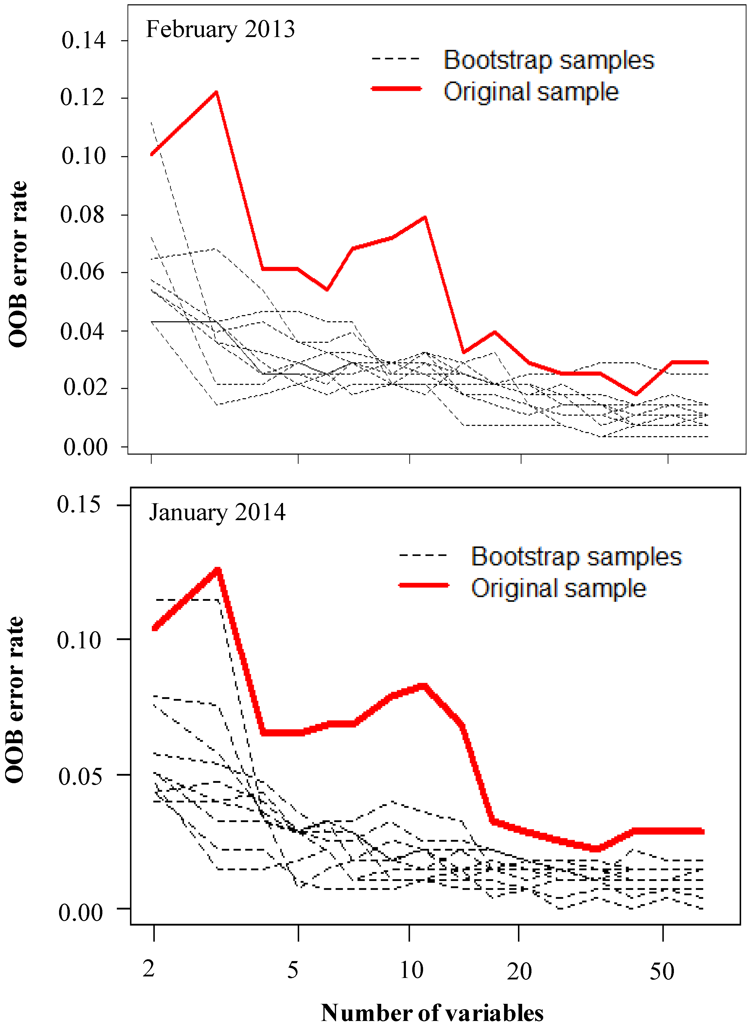
3.1. Optimization of Random Forest Classification Models

An optimal ntree value of 500 was obtained by all RF classification models derived in the present study, while mtry values of 8 and 3 were achieved when classifying the 2013 and the 2014 AISA Eagle image data, respectively. On the other hand, an optimal mtry value of 2 was attained when the important AISA Eagle bands from both the 2013 and the 2014 imagery were analyzed.
Figure 2. The usefulness of AISA Eagle wavebands in classifying the studied classes as measured by the random forest classifier. Bars in red indicate the selected bands (n = 26 for the February 2013 data and n = 21 for the January 2014 data) using the backward selection function and the .632+ bootstrapping rule on the bands importance rank.
Remotesensing 07 13298 g002

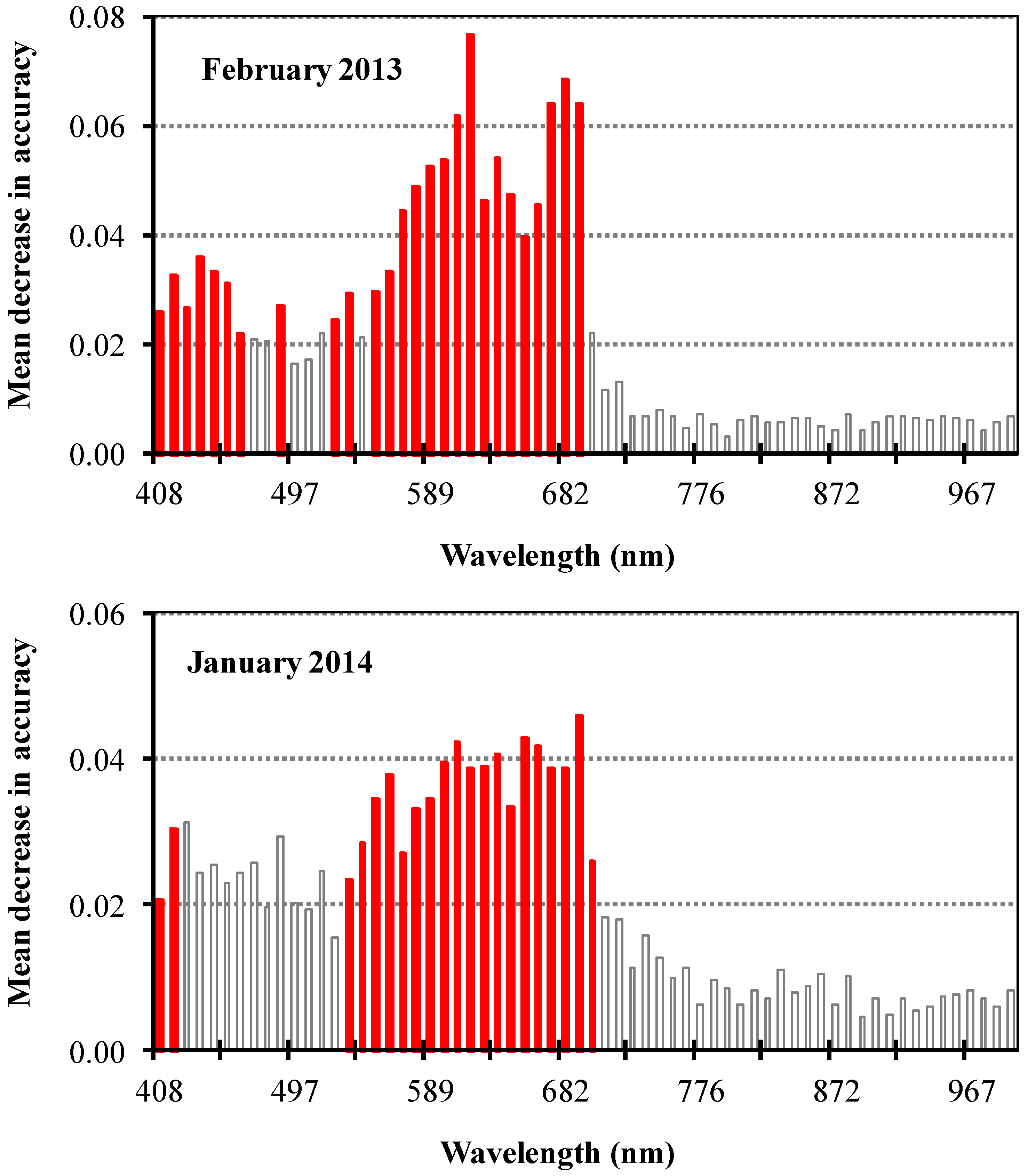
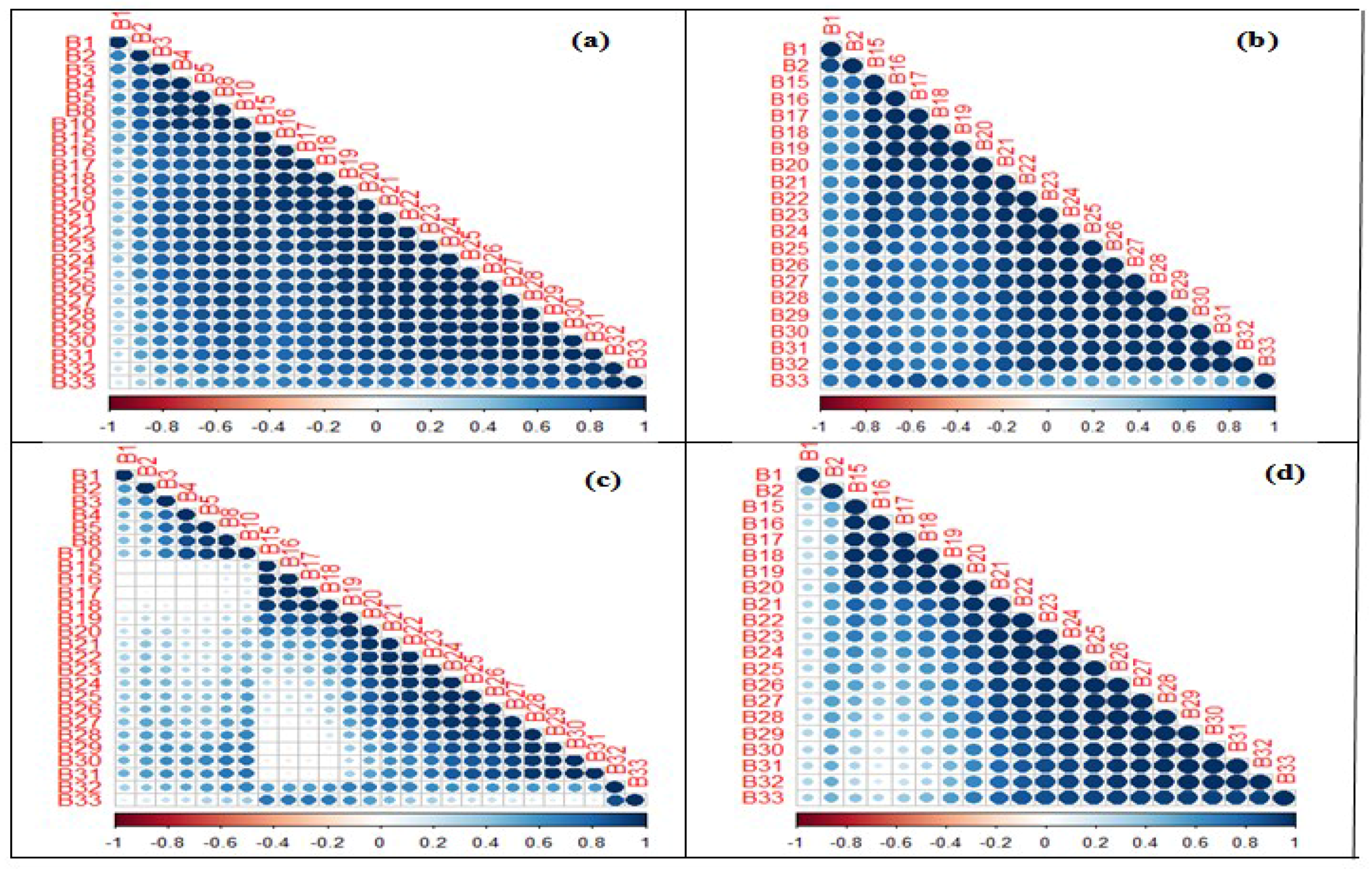
3.2. Spectral Band Selection

The usefulness of the AISA Eagle bands for mapping flowering plants and other LULC classes in the study area using RF is presented in Figure 2. The general trend of band importance in both years (2013 and 2014) was similar. The figure shows that bands centered at the blue (400–500 nm), green (500–600 nm), and red edge (650–690 nm) regions of the electromagnetic spectrum (EMS) were more important for discriminating amongst the classes compared with bands centered at the near infrared spectral region (700–955 nm). Figure 3 shows the change in OOB error rate with increasing number of AISA Eagle spectral bands (n = 64) using the .632+ bootstrap selection method. The method resulted in selecting a fewer number of bands (26 in 2013 and 21 in 2014) that can accurately differentiate among the classes. Figure 2 highlights these useful bands which are located at the visible (400–700 nm) region of the EMS. It is evident that the majorities of these bands are redundant and contain relatively similar spectral information for mapping WF trees as indicated by the Pearson correlation coefficients (r) (Figure 4a,b). While for mapping YF features, co-linearity was observed mainly between adjacent bands (Figure 4c,d).
Figure 3. Results of backward selection function and .632+ bootstrapping rule using AISA Eagle wavebands importance in classifying the studied classes as measured by random forest.
Remotesensing 07 13298 g003
Figure 4. Correlation coefficients (r) between reflectance at the most important AISA Eagle wavebands (n = 26 in February 2013 and 21 in January 2014) when classifying white flowering trees using the February 2013 data (a), the January 2014 data (b) and the yellow flowering trees from the February 2013 data (c) and the January 2014 data (d).
Remotesensing 07 13298 g004

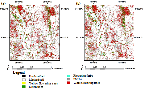
3.3. Accuracy Assessment

The thematic maps produced using AISA Eagle imagery acquired in 2013 and 2014 and RF classification algorithm are presented in Figure 5 and Figure 6. The spatial patterns were different between the maps in that more compact flowering could be visually observed in the 2013 imagery. In January 2014, most of trees in the test site were either green trees or shrubs, with a few scattered WF trees (Figure 6). Croplands (flowering maize and sorghum) were overly present in the 2014 flowering map. The February 2013 data are dominated by the WF class (Figure 5). YF trees were found to be mostly scattered along rivers and seepage lines. It is interesting to note that most of the pixels in the maize and sorghum farms, which were at a senescence stage in February, were masked out as soil and only weeds (forbs) which produced white flowers on the those farms. The confusion matrices of the classification maps (Figure 5 and Figure 6) are shown in Table 2 and Table 3. It is apparent that the OA was considerably different among the maps produced using the AISA Eagle data captured in February 2013 as opposed to those obtained using the January 2014 data. The band selection (variable importance) analysis showed relatively similar classification results compared to those obtained using all AISA Eagle bands. Chi-squared (χ2) of McNemar’s test ranged between 2.01 and 2.56, showing non-significant differences among classification results produced using all AISA Eagle bands and the most important ones. On the contrary, the indvidual accuracies (UA and PA) for most classes were somewhat higher (sometimes 5%–6%) when all AISA Eagle bands were utilized (Table 2 and Table 3). Furthermore, the results showed low QDs (1%–3%) and relatively higher ADs (9%–17%) among the studied classes. However, when assessing the February 2013 RF classification models using the January 2014 data, the OA was quite low (25.13–37.44), indicating poor performance of the models (Table 4).
Figure 5. Classification maps obtained using the random forest classifier, all (a) and the 26 most important (b) AISA Eagle wavebands when data collected in February 2013 were analyzed.
Remotesensing 07 13298 g005
Figure 6. Classification maps obtained using the random forest classifier, all (a) and the 21 most important (b) AISA Eagle wavebands when data collected in January 2014 were analyzed.
Remotesensing 07 13298 g006
Table 2. Classification confusion matrix of random forest classifier using AISA Eagle bands of the 30% test data collected in February 2013.
Ground Truth
(a)
Classified
WFYFGTSHRFBTotalUA
Using all (n= 64) AISA Eagle wavebands
WF46020101035386.79
YF02500100025590.91
GT05035402006484.38
SHR02010154015991.53
FB03020002495687.50
Total5858575955287
PA (%)76.6783.3390.0090.0089.09
OA (%)88.15
QD (%)03.00
AD (%)09.00
(b)Using the most important (n = 26) AISA Eagle wavebands
WF44030202035481.48
YF03490201035884.48
GT04025202006086.67
SHR03020153016088.33
FB04020001485587.27
Total5858585855287
PA (%)73.3381.6786.6788.3387.27
OA (%)85.71
QD (%)01.00
AD (%)13.00
Table 3. Classification confusion matrix of random forest classifier using AISA Eagle bands of the 30% test data collected in January 2014.
Ground Truth
(a)
Classified
WFYFGTSHRCRBTFBTotalUA
Using all (n= 64) AISA Eagle wavebands
WF180101010101012475.00
YF022702020100023675.00
GT020244010001005088.00
SHR010101430001004791.49
CR010200012100022777.78
BT010002010022002684.62
FB000200010200303585.71
Total25355050252535245
PA (%)72.0077.1488.0086.0084.0088.0085.71
OA (%)83.67
QD (%)02.00
AD (%)15.00
(b)WFYFGTSHRCRBTFBTotalUA
Using the most important (n = 21) AISA Eagle wavebands
WF180101010102022669.23
YF022602030200033868.42
GT020243010001004987.76
SHR010202420001004887.50
CR010200012000022676.92
BT010002010021002584.00
FB000200010200283384.85
Total25355050252535245
PA (%)72.0074.2986.0084.0080.0084.0080.00
OA (%)80.82
QD (%)02.00
AD (%)17.00
Table 4. Classification confusion matrix of the random forest model using 70% of the February 2013 data as training data set and 30% of the January 2014 data as independent test sample data set.
Ground Truth
(a)
Classified
WFYFGTSHRFBTotalUA
Using all (n= 64) AISA Eagle wavebands
WF08101507064617.39
YF06121108064327.91
GT04041913044443.18
SHR03050320053655.56
FB04040202142653.85
Total2535505035195
PA (%)13.3320.0031.6733.3340.00
OA (%)37.44
QD (%)18.00
AD (%)45.00
(b)Using the most important (n = 21) AISA Eagle wavebands
WF05121709105309.43
YF06091310074520.00
GT04061416044431.82
SHR06050413063438.24
FB04030202081942.11
Total2535505035195
PA (%)08.3315.0023.3321.6722.86
OA (%)25.13
QD (%)19.00
AD (%)55.00
In general, the individual accuracies (PA and UA) were relatively high; they ranged between 73% and 91.5% for the February 2013 data, while for the January 2014 data the accuracies ranged between 68.42% and 91.5%. The accuracies for WF plants were generally lower than those for YF plants in both data sets, except for the UA when all February 2013 AISA Eagle bands were analyzed. WF trees in January 2014 obtained the least user’s accuracy (69.2), indicating the confusion of this class with other classes. Contrary, all classes were inaccurately mapped (low PA and UA were obtained) when the February 2013 classification models were transferred to the January 2014 data (Table 4).

4. Discussion

The results showed relatively high OA and individual class accuracies (PA, and UA), indicating the potential of AISA Eagle data and RF classifier for flower mapping in a heterogeneous landscape. Furthermore, our study showed the robustness of the .632+ bootstrap method of the RF classifier in reducing the dimensionality of the hyperspectral data.
The optimal ntree values (500) for RF classification models developed in the present study were consistent with the default value recommended by Breiman [37]. While, only the analysis of 2013 AISA Eagle bands resulted in a default mtry value (8) which is the square root of the predictor variables [37]. However, RF is an empirical machine learning method that requires optimized ntree and mtry parameters (e.g., [38,53]).
We have masked out bare soil areas and produced an explicit flowering and LULC maps showing only vegetation classes (Figure 5 and Figure 6). It is therefore expected that bands in the visible portion of the EMS were found to be more useful for feature and land cover class discrimination [26]. The SWIR region of the EMS could have been useful for discriminating different flowering plants. However, using SWIR bands would have increased the AISA Eagle image acquisition costs significantly as we would have needed to fly at a three times lower altitude in order to capture the same pixel size, due to SWIR sensor specifications. Having visible and near infrared (VINIR) and SWIR spectral regions would always be useful, but in our case the VNIR spectral region was optimally sufficient to separate flowering from non-flowering and also discriminate between flowering colors [54]. Spectral characteristics in the visible and red edge waveband regions are known to be sensitive to chlorophyll and other leaf and flower pigments [9,55]. In addition, the results showed that decreasing the dimensionality (26 bands in 2013 and 21 bands in 2014) produced relatively similar accuracies compared to all the bands (n = 64). The dimensionality of the AISA Eagle was reduced by about 40% and 33% for 2013 and 2014 data, respectively. It is also worth noting that the computational cost of optimizing the RF classification algorithm using grid search and a cross-validation method was considerably decreased when the dimensionality of the hyperspectral data was reduced. However, some of the selected bands were found to be correlated and contain the same spectral information, particularly for mapping WF trees. Therefore, future studies should employ classification methods that take into account the co-linearity between the predictor bands like Deng and Runger’s [47] regularized RF classification algorithm.
OA achieved in the present study are comparable to the recommendation of Anderson et al. [56] who noted that any OA mapping result less than 80%, for particular features and classes mapped using remotely sensed data, cannot be considered accurate. Nonetheless, the relatively high OA presented in Table 2 and Table 3 should be interpreted with some caution; the high OA might not represent the true accuracy of the classification maps [57]. The individual class accuracies for some classes like WF trees are relatively low. This could be due to the confusion of WF plant canopies with background soil reflectance particularly along the perimeter of plant canopies [8]. The low mapping accuracy for WF class could also be explained by the slightly higher auto-correlation between the useful bands (Figure 4). The lower correlation coefficients between the optimized bands as a function of mapping YF (Figure 4c,d), compared to mapping WF (Figure 4a,b), provided a further insight into the higher classification accuracy of the YF class. These discrepancies in correlations between the optimized bands for mapping the YF and the WF classes need further investigation. In general, the spatial patterns of the flowering plants in the two maps (Figure 5 and Figure 6) are somewhat different. These differences are a result of differences in flowering fractional coverages between January (beginning of blooming) and February (peak blooming period). For example, the upper left and upper right and bottom right patches in January 2014 (Figure 6) were white flowering plants in February 2013 (Figure 5). Since we used canopy-level hyperspectral data, the shape and geometry of flowering tree species could have affected the spectral responses of flowering classes [9,58] and hence the mapping accuracy of these classes. We applied a pixel-based classification approach which often leads to a “salt-and-pepper” pattern in the mapping result [59,60,61]. Likewise, Cho et al. [12] noted that such an approach can result in misclassification of pixels along the border of the tree crowns and within the tree crown, particularly for the trees that have high intra-class variability. Since flower mapping requires high spatial resolution imagery to capture flowering responds within plants and tree canopies [8], we suggest that the methods used in our study could only be up-scaled to spaceborne images of about one meter pixel resolution. However, most satellite-borne images of a very fine pixel size (~1 m) deem to exhibit multispectral data characteristics (e.g., WorldView-3) with a few number of bands that might not be adequate for discriminating flowering responds. We utilized hyperspectral data with a fine spatial resolution (0.6 m) in combination with an optimized machine learning classification approach (RF) which would have been sufficient in mapping the flowering plants even if they were not in bloom at the time the images were acquired. However, our initial aim was to produce flowering maps in two different time points that could be useful in assessing floral change (i.e., phenology). We also conducted our experiment in February 2013 which is the maximum flowering period. The maximum flowering period is more significant for hive productivity and honey flow since flowering trees that are preferred by bees (i.e., Acacia tortilis) are in full bloom during this period [3]. We then repeated the experiment at the beginning of the flowering period (January 2014) to assess the applicability of our methods using field data of less floral fractional coverage. In particular, we grouped the flowering plants in the study area according to their flowering colors (i.e., white and yellow) and mapped the flowering plants to provide information that is helpful for making informed decisions regarding the optimal placement of bee hives in the landscape and to better understand honeybees’ foraging behavior. Nevertheless, the future studies should incorporate the SWIR bands together with the VNIR and explore the utility of AISA Eagle hyperspectral data and optimized random forest classification method for mapping the relevant plant species when they are not in full bloom (green trees). The upcoming studies should also look at up-scaling the approach for mapping the plant species when they are not blooming to speceborne hyperspectral sensors.
Our study also showed that flowering classes can be mapped more accurately in the February 2013 data than in the January 2014 data. In general, February is the peak flowering period when most of the melliferous plants at the Mwingi study area are in full bloom, while January is the beginning of blooming period. These seasonal differences are largely associated with flowering compaction, the effect of non-flowering material on the flower signal that is received by the sensor, and phenological variations between the same tree species. The seasonal and phenological differences between the two data sets (February 2013 and January 2014) could also be a reason for the the poor performance of February 2013 models when transferred to the January 2014 data. Another reason that could have hindered the performance of the February 2013 models, when up-scaled in time (Table 4), is the collinearity between the predictor variables (AISA Eagle bands). This is in acordance with the finding of Dormann et al. [62] who noted that collinearity can hinder the performance of statistical models when transferred to other points in time or space. Furthermore, the results of the current study showed that YF trees are mainly found along the riverside vegetation communities. This finding could be further investigated to study the effect of topography and proximity from rivers in mapping the spatial distribution of flowering plants.
We mapped the spatial distribution and abundance of YF and WF plants in the landscape matrix. This information is required for understanding honeybees’ foraging behavior [63] as an important measure for developing conservation frameworks for bee diversity, bee health, and landscape integrity [64]. Spatio-temporal information about melliferous plants is also valuable for conservation and ecological status valuations and ultimately sustainable resource use and biodiversity [65].

5. Conclusions

This study demonstrated the possibility of mapping flowering features and other LULC types in a heterogeneous landscape using AISA Eagle hyperspectral data. Maps derived for the peak flowering season were more accurate than those derived for the beginning of the main flowering period. Despite the fact that most of the white flowering crops were not existent (already harvested cropland) in February 2013, we recommend the use of the February 2013 data set for modeling purposes (e.g., analyzing the abundance and distribution of flowering plants for landscape and bee health studies). The spatial flowering patterns observed in February 2013 were somewhat more compact compared to the patterns in January 2014. Furthermore, in Kenya farmers’ decision regarding the planting date of crops (which is a land use class in the January 2014 map) and the cropping system used in a particular year is highly variable and depends on socio-economic and climatic factors. Random forest .632+ bootstrapping feature selection method proved useful in reducing the dimensionality of hyperspectral data. The selected bands produced maps of comparable accuracies to those produced using all AISA Eagle bands. However, most of the selected AISA Eagle bands were redundant and auto-correlated, hence future studies should look at the use of classification methods that do not encounter auto-correlation problems such as the regularized RF classification algorithm.
Overall, our study is an important step towards a development of an operational flower mapping framework in African savannas. Given the cost of AISA Eagle data and cloud cover which might hinder acquisition of cloud-free spaceborne images during specific phenological flowering stage, the future studies should investigate the use of hyperspectral sensors mounted on drones or unmanned aerial vehicles for mapping flowering response and explicit LULC assessments. However, if cloud-free satellite imagery of high spatial resolutions (e.g., WorldView-3) can be acquired, the methods used in our study could be extended to spaceborne sensors so that monitoring of floral cycles at key sites can be facilitated at regular intervals.

Acknowledgments

We thank the European Union for funding of the project “African reference laboratory for the management of pollinator bee diseases and pests for food security” in which context the present study was made possible. We are grateful to the University of Helsinki, Department of Geoscience and Geography, for capturing the hyperspectral data and data pre-processing. We also thank bee keepers in Mwingi, Kenya for facilitating field data collection. We gratefully acknowledge the Centre for International Migration and Development (CIM) of the German Development Organization (GIZ). We also acknowledge the contribution of the International Center for Insect Physiology and Ecology (ICIPE) “Random Forest Innovations Project”. Our gratitude is further extended to the Faculty of Agriculture, University of Khartoum. We are very thankful to the anonymous reviewers for their useful comments and suggestions.

Author Contributions

Elfatih M. Abdel-Rahman analyzed the data, wrote the manuscript and is the main author of all sections. All co-authors provided valuable inputs with regard to fieldwork, data analysis, and manuscript preparation.

Conflicts of Interest

The authors declare no conflict of interest.

References

  1. Sammataro, D.; Weiss, M. Comparison of productivity of colonies of honey bees, Apis mellifera, supplemented with sucrose or high fructose corn syrup. J. Insect Sci. 2013, 13. [Google Scholar] [CrossRef] [PubMed]
  2. Sponsler, D.B.; Johnson, R.M. Honey bee success predicted by landscape composition in Ohio, USA. PeerJ 2015, 3. [Google Scholar] [CrossRef] [PubMed]
  3. Raina, S.K.; Kioko, E.; Zethner, O.; Wren, S. Forest habitat conservation in Africa using commercially important insects. Annu. Rev. Entomol. 2011, 56, 465–485. [Google Scholar] [CrossRef] [PubMed]
  4. Chen, J.; Shen, M.; Zhu, X.; Tang, Y. Indicator of flower status derived from in situ hyperspectral measurement in an alpine meadow on the Tibetan Plateau. Ecol. Indic. 2009, 9, 818–823. [Google Scholar] [CrossRef]
  5. Decourtye, A.; Mader, E.; Desneux, N. Landscape enhancement of floral resources for honey bees in agro-ecosystems. Apidologie 2010, 41, 264–277. [Google Scholar] [CrossRef]
  6. Fitter, A.; Fitter, R. Rapid changes in flowering time in British plants. Science 2002, 296, 1689–1691. [Google Scholar] [CrossRef] [PubMed]
  7. Houle, G. Spring-flowering herbaceous plant species of the deciduous forests of eastern Canada and 20th century climate warming. Can. J. For. Res. 2007, 37, 505–512. [Google Scholar] [CrossRef]
  8. Landmann, T.; Piiroinen, R.; Makori, D.M.; Abdel-Rahman, E.M.; Makau, S.; Pellikka, P.; Raina, S.K. Application of hyperspectral remote sensing for flower mapping in African savannas. Remote Sens. Environ. 2015, 166, 50–60. [Google Scholar] [CrossRef]
  9. Kumar, L.; Dury, S.J.; Schmidt, K.; Skidmore, A. Imaging spectrometry and vegetation science. In Image Spectrometry; van der Meer, F.D., de Jong, S.M., Eds.; Kluwer Academic Publishers: London, UK, 2003; pp. 111–156. [Google Scholar]
  10. Lillesand, T.M.; Kiefer, R.W. Remote Sensing and Image Interpretation, 4th ed.; John Wiley & Sons Inc.: New York, NY, USA, 2001. [Google Scholar]
  11. Naidoo, L.; Cho, M.; Mathieu, R.; Asner, G. Classification of savanna tree species, in the Greater Kruger National Park region, by integrating hyperspectral and LiDAR data in a Random Forest data mining environment. ISPRS J. Photogramm. Remote Sens. 2012, 69, 167–179. [Google Scholar] [CrossRef]
  12. Cho, M.A.; Mathieu, R.; Asner, G.P.; Naidoo, L.; van Aardt, J.; Ramoelo, A.; Debba, P.; Wessels, K.; Main, R.; Smit, I.P. Mapping tree species composition in South African savannas using an integrated airborne spectral and LiDAR system. Remote Sens. Environ. 2012, 125, 214–226. [Google Scholar] [CrossRef]
  13. Giurfa, M.; Nunez, J.; Chittka, L.; Menzel, R. Colour preferences of flower-naive honeybees. J. Comp. Physiol. 1995, 177, 247–259. [Google Scholar] [CrossRef]
  14. Cnaani, J.; Thomson, J.D.; Papaj, D.R. Flower choice and learning in foraging bumblebees: Effects of variation in nectar volume and concentration. Ethology 2006, 112, 278–285. [Google Scholar] [CrossRef]
  15. Weng, Q. Advances in Environmental Remote Sensing: Sensors, Algorithms, and Applications; CRC Press: Boca Raton, FL, USA, 2011. [Google Scholar]
  16. Thenkabail, P.S.; Lyon, J.G.; Huete, A. Hyperspectral Remote Sensing of Vegetation; CRC Press: Boca Raton, FL, USA, 2011. [Google Scholar]
  17. Christian, B.; Krishnayya, N. Classification of tropical trees growing in a sanctuary using Hyperion (EO-1) and SAM algorithm. Curr. Sci. 2009, 96, 1601–1607. [Google Scholar]
  18. Féret, J.; Asner, G.P. Tree species discrimination in tropical forests using airborne imaging spectroscopy. IEEE Trans. Geosci. Remote Sens. 2013, 51, 73–84. [Google Scholar] [CrossRef]
  19. Prospere, K.; McLaren, K.; Wilson, B. Plant species discrimination in a tropical wetland using in situ hyperspectral data. Remote Sens. 2014, 6, 8494–8523. [Google Scholar] [CrossRef]
  20. Plaza, A.; Benediktsson, J.A.; Boardman, J.W.; Brazile, J.; Bruzzone, L.; Camps-Valls, G.; Chanussot, J.; Fauvel, M.; Gamba, P.; Gualtieri, A. Recent advances in techniques for hyperspectral image processing. Remote Sens. Environ. 2009, 113, S110–S122. [Google Scholar] [CrossRef]
  21. Ham, J.; Chen, Y.; Crawford, M.; Ghosh, J. Investigation of the random forest framework for classification of hyperspectral data. IEEE Trans. Geosci. Remote Sens. 2005, 43, 492–501. [Google Scholar] [CrossRef]
  22. Lawrence, R.L.; Wood, S.D.; Sheley, R.L. Mapping invasive plants using hyperspectral imagery and Breiman Cutler classifications (randomForest). Remote Sens. Environ. 2006, 100, 356–362. [Google Scholar] [CrossRef]
  23. Chan, J.C.W.; Paelinckx, D. Evaluation of Random Forest and Adaboost tree-based ensemble classification and spectral band selection for ecotope mapping using airborne hyperspectral imagery. Remote Sens. Environ. 2008, 112, 2999–3011. [Google Scholar] [CrossRef]
  24. Waske, B.; Benediktsson, J.A.; Ãrnason, K.; Sveinsson, J.R. Mapping of hyperspectral AVIRIS data using machine-learning algorithms. Can. J. Remote Sens. 2009, 35, 106–116. [Google Scholar] [CrossRef]
  25. Ramoelo, A.; Skidmore, A.; Cho, M.; Mathieu, R.; Heitkönig, I.; Dudeni-Tlhone, N.; Schlerf, M.; Prins, H. Non-linear partial least square regression increases the estimation accuracy of grass nitrogen and phosphorus using in situ hyperspectral and environmental data. ISPRS J. Photogramm. Remote Sens. 2013, 82, 27–40. [Google Scholar] [CrossRef]
  26. Abdel-Rahman, E.M.; Mutanga, O.; Adam, E.; Ismail, R. Detecting Sirex noctilio grey-attacked and lightning-struck pine trees using airborne hyperspectral data, random forest and support vector machines classifiers. ISPRS J. Photogramm. Remote Sens. 2014, 88, 48–59. [Google Scholar] [CrossRef]
  27. Ngugi, R.K. Use of Indigenous and Contemporary Knowledge on Climate and Drought Forecasting Information in Mwingi District, Kenya; A Report to UNDP; College of Agriculture and Veterinary Science, University of Nairobi: Nairobi, Kenya, 1999. [Google Scholar]
  28. Raina, S.; Kimbu, D. Variations in races of the honeybee Apis mellifera (Hymenoptera: Apidae) in Kenya. Int. J. Trop. Insect Sci. 2005, 25, 281–291. [Google Scholar] [CrossRef]
  29. Delaplane, K.S. Honey Bees and Beekeeping; A Report of Cooperative Extension; College of Agricultural and Environmental Sciences, College of Family and Consumer Sciences, The University of Georgia: Athens, GA, USA, 2010. [Google Scholar]
  30. Williams, G.R.; Tarpy, D.R.; Vanengelsdorp, D.; Chauzat, M.P.; Cox-Foster, D.L.; Delaplane, K.S.; Neumann, P.; Pettis, J.S.; Rogers, R.E.; Shutler, D. Colony collapse disorder in context. Bioessays 2010, 32, 845–846. [Google Scholar] [CrossRef] [PubMed]
  31. Fening, K.O.; Kioko, E.N.; Raina, S.K.; Mueke, J.M. Monitoring wild silkmoth, Gonometa postica Walker, abundance, host plant diversity and distribution in Imba and Mumoni woodlands in Mwingi, Kenya. Int. J. Biodivers. Sci. Manage. 2008, 4, 104–111. [Google Scholar] [CrossRef]
  32. Muya, B.I. Determinants of Adoption of Modern Technologies in Beekeeping Projects: The Case of Women Groups in Kajiado County, Kenya. Master’s Thesis, University of Nairobi, Nairobi, Kenya, 2014. [Google Scholar]
  33. Gao, B.C.; Montes, M.J.; Davis, C.O.; Goetz, A.F. Atmospheric correction algorithms for hyperspectral remote sensing data of land and ocean. Remote Sens. Environ. 2009, 113, S17–S24. [Google Scholar] [CrossRef]
  34. Richter, R.; Schläpfer, D. Geo-atmospheric processing of airborne imaging spectrometry data. Part 2: Atmospheric/topographic correction. Int. J. Remote Sens. 2002, 23, 2631–2649. [Google Scholar] [CrossRef]
  35. Guanter, L.; Richter, R.; Kaufmann, H. On the application of the MODTRAN4 atmospheric radiative transfer code to optical remote sensing. Int. J. Remote Sens. 2009, 30, 1407–1427. [Google Scholar] [CrossRef]
  36. Mannschatz, T.; Pflug, B.; Borg, E.; Feger, K.-H.; Dietrich, P. Uncertainties of LAI estimation from satellite imaging due to atmospheric correction. Remote Sens. Environ. 2014, 153, 24–39. [Google Scholar] [CrossRef]
  37. Breiman, L. Random forests. Mach. Learn. 2001, 45, 5–32. [Google Scholar] [CrossRef]
  38. Liaw, A.; Weiner, M. Classification and regression by randomForest. R News. 2002, 2, 18–22. [Google Scholar]
  39. Statnikov, A.; Wang, L.; Aliferis, C.F. A comprehensive comparison of random forests and support vector machines for microarray-based cancer classification. BMC Bioinf. 2008, 9, 1–10. [Google Scholar] [CrossRef] [PubMed]
  40. Prasad, A.; Iverson, L.; Liaw, A. Newer classification and regression tree techniques: Bagging and random forests for ecological prediction. Ecosystems 2006, 9, 181–199. [Google Scholar] [CrossRef]
  41. Guo, L.; Chehata, N.; Mallet, C.; Boukir, S. Relevance of airborne lidar and multispectral image data for urban scene classification using Random Forests. ISPRS J. Photogramm. Remote Sens. 2011, 66, 56–66. [Google Scholar] [CrossRef]
  42. Qi, Y. Random forest for bioinformatics. In Ensemble Machine Learning: Methods and Applications; Zhang, C., Ma, Y., Eds.; Springer: Berlin, Germany, 2012; pp. 307–323. [Google Scholar]
  43. R Development Core Team. R: A Language and Environment for Statistical Computing, R Foundation for Statistical Computing. Available online: http://www.R-project.org (accessed on 20 April 2015).
  44. Diaz-Uriarte, R. Package “varSelRF”. Available online: http://ligarto.org/rdiaz/Software/Software.html (accessed on 20 April 2015).
  45. Efron, B.; Tibshirani, R. Improvements on cross-validation: The .632+ bootstrap method. J. Am. Stat. Assoc. 1997, 92, 548–560. [Google Scholar]
  46. Diaz-Uriarte, R.; Alvarez de Andres, S. Gene selection and classification of microarray data using random forest. BMC Bioinf. 2006, 7, 1–13. [Google Scholar]
  47. Deng, H.; Runger, G. Feature selection via regularized trees. In Proceedings of the 2012 International Joint Conference on Neural Networks (IJCNN), Brisbane, QLD, Australia, 10–15 June 2012.
  48. Adam, E.; Mutanga, O.; Ismail, R. Determining the susceptibility of Eucalyptus nitens forests to Coryphodema tristis (cossid moth) occurrence in Mpumalanga, South Africa. Int. J. Geogr. Inf. Sci. 2013, 27, 1924–1938. [Google Scholar] [CrossRef]
  49. Cohen, J.A. Coefficient of agreement for nominal scales. Educ. Psychol. Meas. 1960, 20, 37–46. [Google Scholar] [CrossRef]
  50. Congalton, R.G.; Green, K. Assessing the Accuracy of Remotely Sensed Data: Principles and Practices; Lewis Publishers: Boca Raton, FL, USA, 1999. [Google Scholar]
  51. Pontius, R.G.; Millones, M. Death to Kappa: Birth of quantity disagreement and allocation disagreement for accuracy assessment. Int. J. Remote Sens. 2011, 32, 4407–4429. [Google Scholar] [CrossRef]
  52. Foody, G.M. Thematic map comparison: Evaluating the statistical significance of differences in classification accuracy. Photogramm. Eng. Remote Sens. 2004, 70, 627–633. [Google Scholar] [CrossRef]
  53. Abdel-Rahman, E.M.; Ahmed, F.B.; Ismail, R. Random forest regression and spectral band selection for estimating sugarcane leaf nitrogen concentration using EO-1 Hyperion hyperspectral data. Int. J. Remote Sens. 2013, 34, 712–728. [Google Scholar] [CrossRef]
  54. Ge, S.; Everitt, J.; Carruthers, R.; Gong, P.; Anderson, G. Hyperspectral characteristics of canopy components and structure for phenological assessment of an invasive weed. Environ. Monit. Assess. 2006, 120, 109–126. [Google Scholar] [CrossRef] [PubMed]
  55. Filella, I.; Penuelas, J. The red edge position and shape as indicators of plant chlorophyll content, biomass and hydric status. Int. J. Remote Sens. 1994, 15, 1459–1470. [Google Scholar] [CrossRef]
  56. Anderson, J.R.; Hardy, E.E.; Roach, J.T.; Witmer, R.E. A Land Use and Land Cover Classification System for Use with Remote Sensor Data; US Government Printing Office: Washington, DC, USA, 1976; Volume 964. [Google Scholar]
  57. Olofsson, P.; Foody, G.M.; Stehman, S.V.; Woodcock, C.E. Making better use of accuracy data in land change studies: Estimating accuracy and area and quantifying uncertainty using stratified estimation. Remote Sens. Environ. 2013, 129, 122–131. [Google Scholar] [CrossRef]
  58. Petropoulos, G.P.; Manevski, K.; Carlson, T.N. Hyperspectral remote sensing with emphasis on land cover mapping: From ground to satellite observations. In Scale Issues in Remote Sensing; Weng, Q., Ed.; John Wiley & Sons Inc.: Oxford, UK, 2014; pp. 285–320. [Google Scholar]
  59. De Jong, S.M.; Hornstra, T.; Maas, H.G. An integrated spatial and spectral approach to the classification of Mediterranean land cover types: The SSC method. Int. J. Appl. Earth Obs. Geoinf. 2001, 3, 176–183. [Google Scholar] [CrossRef]
  60. Ouyang, Z.T.; Zhang, M.Q.; Xie, X.; Shen, Q.; Guo, H.Q.; Zhao, B. A comparison of pixel-based and object-oriented approaches to VHR imagery for mapping saltmarsh plants. Ecol. Inform. 2011, 6, 136–146. [Google Scholar] [CrossRef]
  61. Piiroinen, R.; Heiskanen, J.; Mõttus, M.; Pellikka, P. Classification of crops across heterogeneous agricultural landscape in Kenya using AisaEAGLE imaging spectroscopy data. Int. J. Appl. Earth Obs. Geoinf. 2015, 39, 1–8. [Google Scholar] [CrossRef]
  62. Dormann, C.F.; Elith, J.; Bacher, S.; Buchmann, C.; Carl, G.; Carré, G.; Marquéz, J.R.G.; Gruber, B.; Lafourcade, B.; Leitão, P.J. Collinearity: A review of methods to deal with it and a simulation study evaluating their performance. Ecography 2013, 36, 27–46. [Google Scholar] [CrossRef]
  63. Dongock, N.; Tchoumboue, J.; Youmbi, E.; Zapfack, L.; Mapongmentsem, P.; Tchuenguem, F. Predominant melliferous plants of the western Sudano Guinean zone of Cameroon. AJEST 2011, 5, 443–447. [Google Scholar]
  64. Abou-Shaara, H. Continuous management of varroa mite in honey bee, Apis. mellifera, colonies. Acarina 2014, 22, 149–156. [Google Scholar]
  65. Tashev, A.; Pancheva, E. The Melliferous plants of the Bulgarian flora—Conservation importance. For. Ideas 2011, 17, 228–237. [Google Scholar]

