Article

First Polarimetric GNSS-R Measurements from a Stratospheric Flight over Boreal Forests

Barcelona Tech Remote Sensing Laboratory and IEEC/UPC, Universitat Politècnica de Catalunya, UPC Campus Nord, D3, Barcelona 08034, Spain
*
Author to whom correspondence should be addressed.
Remote Sens. 2015, 7(10), 13120-13138; https://doi.org/10.3390/rs71013120
Submission received: 29 June 2015 / Revised: 18 September 2015 / Accepted: 27 September 2015 / Published: 2 October 2015

Abstract

:
The first-ever dual-frequency multi-constellation Global Navigation Satellite Systems Reflectometry (GNSS-R) polarimetric measurements over boreal forests and lakes from the stratosphere are presented. Data were collected during the Swedish National Space Board (SNSB)/European Space Agency (ESA) sponsored Balloon Experiments for University Students (BEXUS) 19 stratospheric balloon experiment using the P(Y) and C/A ReflectOmeter (PYCARO) instrument operated in closed-loop mode. Maps of the polarimetric ratio for L1 and L2 Global Positioning System (GPS) and GLObal Navigation Satellite System (GLONASS), and for E1 Galileo signals are derived from the float phase at 27,000 m height, and the specular points are geolocalized on the Earth’s surface. Polarimetric ratio (Γrlrr) maps over boreal forests are shown to be in the range 2–16 dB for the different GNSS codes. This result suggests that the scattering is taking place not only over the soil, but over the different forests elements as well. Additionally to the interpretation of the experimental results a theoretical investigation of the different contributions to the total reflectivity over boreal forests is performed using a bistatic scattering model. The simulated cross- (reflected Left Hand Circular Polarization LHCP) and co-polar (reflected Right Hand Circular Polarization RHCP) reflectivities are evaluated for the soil, the canopy, and the canopy–soil interactions for three different biomass densities: 725 trees/ha, 150 trees/ha and 72 trees/ha. For elevation angles larger than the Brewster angle, it is found that the cross-polar signal is dominant when just single reflections over the forests are evaluated, while in the case of multiple reflections the co-polar signal becomes the largest one.

Graphical Abstract

1. Introduction

Scientific applications of GNSS-R for Earth Observation include mesoscale ocean altimetry [1], wind speed measurements [2], ice altimetry [3], and soil moisture and vegetation determination [4]. There are different data acquisition techniques [5]: Conventional GNSS-R (cGNSS-R) [6], interferometric GNSS-R (iGNSS-R) [7], and reconstructed-code GNSS-R (rGNSS-R) [8]. At present, data collected by the Surrey Satellite Technology Ltd SSTL’s TechDemoSat-1 mission [9] are being processing by the community. Scattering over ocean is found to be highly diffuse, while over land and cryosphere surface targets the reflection becomes specular [10]. These studies consolidate the pioneer results of the United Kingdom Disaster Monitoring Constellation (UK-DMC) and push forward the popularity of GNSS-R in the Remote Sensing community. In the near future several new space-borne missions will include GNSS-R payloads: National Aeronautics and Space Administration (NASA) Cyclone Global Navigation Satellite System (GyGNSS) mission [11], ESA’s GNSS rEflectometry, Radio Occultation and Scatterometry experiment on-board the International Space Station (GEROS-ISS) [12], ESA’s Passive Reflectometry and Interferometry System In-Orbit Demonstrator (PARIS-IoD) [13], and UPC’s 3Cat-2 6U CubeSat [14].
The use of GNSS-R polarimetry over land was first proposed in 2000 for soil moisture monitoring [15]. Later, theoretical simulations were carried out to evaluate the performance of GNSS-R polarimetric measurements for biomass monitoring [16]. Coherent and incoherent scattering were considered in the simulations. In particular, the coherent electromagnetic field was modeled as the reflection of the GNSS signals over the soil, attenuated by the vegetation above it. In this work [16], it was stated that the coherent component of the co-polar reflected signal is 30 dB lower than the cross-polar one. The incoherent component is dominant for co-polar signatures and for a biomass density larger than 50 ton/ha, while the coherent component is the highest for cross-polar signals up to 200 t/ha. Later, an experimental study [17] showed that the co-polar coherent reflectivity is roughly constant for biomass densities from 100 t/ha to 350 t/ha and for an elevation angle in the range θe = (50°, 80°). On the other side, the cross-polar component is shown to be reduced to approximately 5 dB. Recently, a different approach has proposed that the forward scattering coefficient is governed by the scattering properties of the vegetation elements and the soil surface, as well as by the interaction between the canopy and the soil, and the soil with the trunks [18]. In this study, the total cross- and the co-polar scattering coefficients are shown to be, respectively, approximate −8 to 8 dB, and approximate −2 to −15 dB for elevation angles in the range θe = (50°, 80°).
This work presents the first-ever measurements of polarimetric GNSS-R signatures using data from a stratospheric balloon experiment. Section 2 describes the experimental set-up. Section 3 presents the experimental results obtained with the PYCARO instrument and their interpretation. Section 4 provides final discussions, and conclusions are included in Section 5. Additionally, theoretical simulations of the cross- and co-polar reflectivities are presented in the appendix. The EMISVEG simulator [19,20] uses a bistatic scattering model to evaluate separately the forward scattered field over the soil, and the different forest’s trees elements.

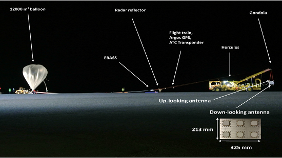
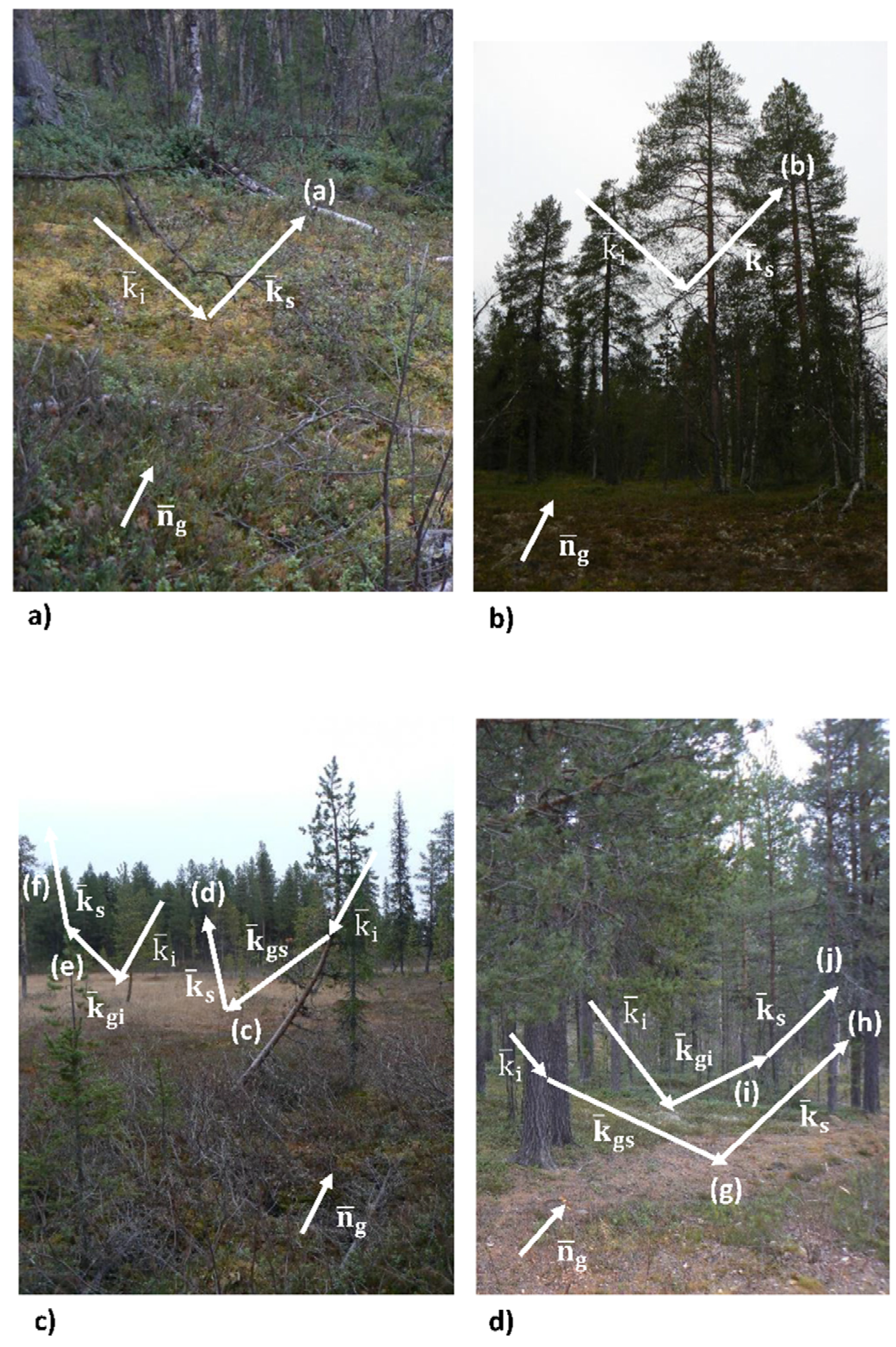
2. Experimental Set-Up and Scenario

The ESA BEXUS 19 stratospheric flight (Figure 1) took place on 8 October 2014, at 6:00 p.m. (GPS Time), the experiment duration was 4 hours, the maximum flight height was ~27,000 m, and the trajectory was a single track from Esrange Space Center (latitude 67°53′N, longitude 21°04′E) to Finland (latitude 68°04′N, longitude 25°81′E) over lakes and boreal forest, which is characterized by coniferous forests consisting mostly of pines, spruces, and larches with needle-shaped leaves. Note that biomass of boreal forests is high, but the plant species diversity is less than that in tropical wet forests. The structure of these forests is quite homogeneous which allows the use of allometric equations to characterize the biomass. An updated version of the PYCARO reflectometer [8] including GLONASS and Galileo correlation channels was used. Additionally, both dual-band (L1, L2) and dual-polarization (RHCP, LHCP) zenith-looking antenna patch to collect the direct GNSS signals and nadir-looking antenna array to collect the Earth-reflected signals (Figure 1) were installed in the gondola. The nadir-looking antenna was composed of 6 elementary antenna patches. The total gain of the array was 12.9 dB at L1-LHCP, 13.3 dB at L1-RHCP, 11.6 dB at L2-LHCP and 11.6 dB at L2-RHCP. The On-Board Data Handling (OBDH) subsystem was composed of a Commercial Off The Shelf (COTS) microcontroller for housekeeping and scientific data management, communications with the ground station, and data storage in a micro-Secure Digital (SD) card. The collected data were registered on-board, and simultaneously they were sent to the ground station using the E-Link system [21]. Additionally, an active thermal control was used because the outdoor temperature was so cold down to −70 °C.
Figure 1. Configuration of the BEXUS 19 stratospheric balloon at Esrange Space Center: 12,000 m3 balloon, valve, cutter, parachute, Esrange Balloon Service System (EBASS), flight train, Argos GPS and Air Traffic Control (ATC) Transponder (AGT), strobe light, radar reflector, and gondola. Total length of the system is up to 75 m [21]. Photo credits: European Space Agency (ESA).
Remotesensing 07 13120 g001

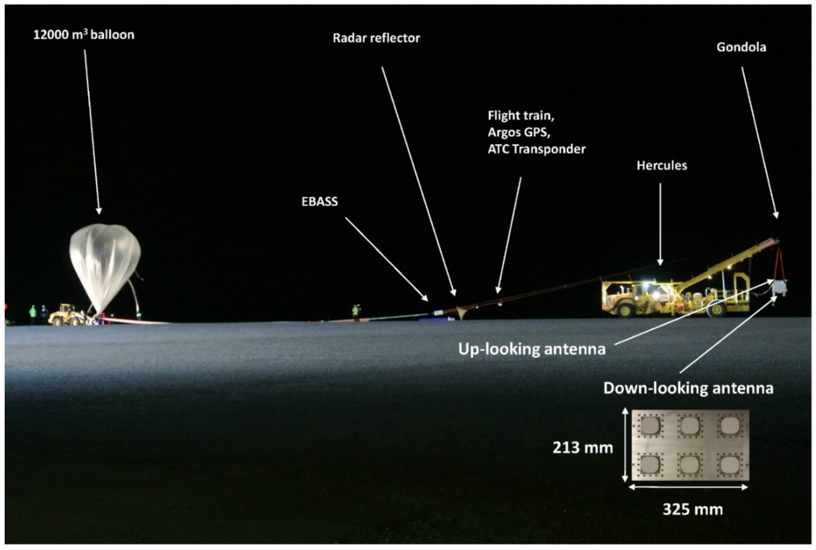
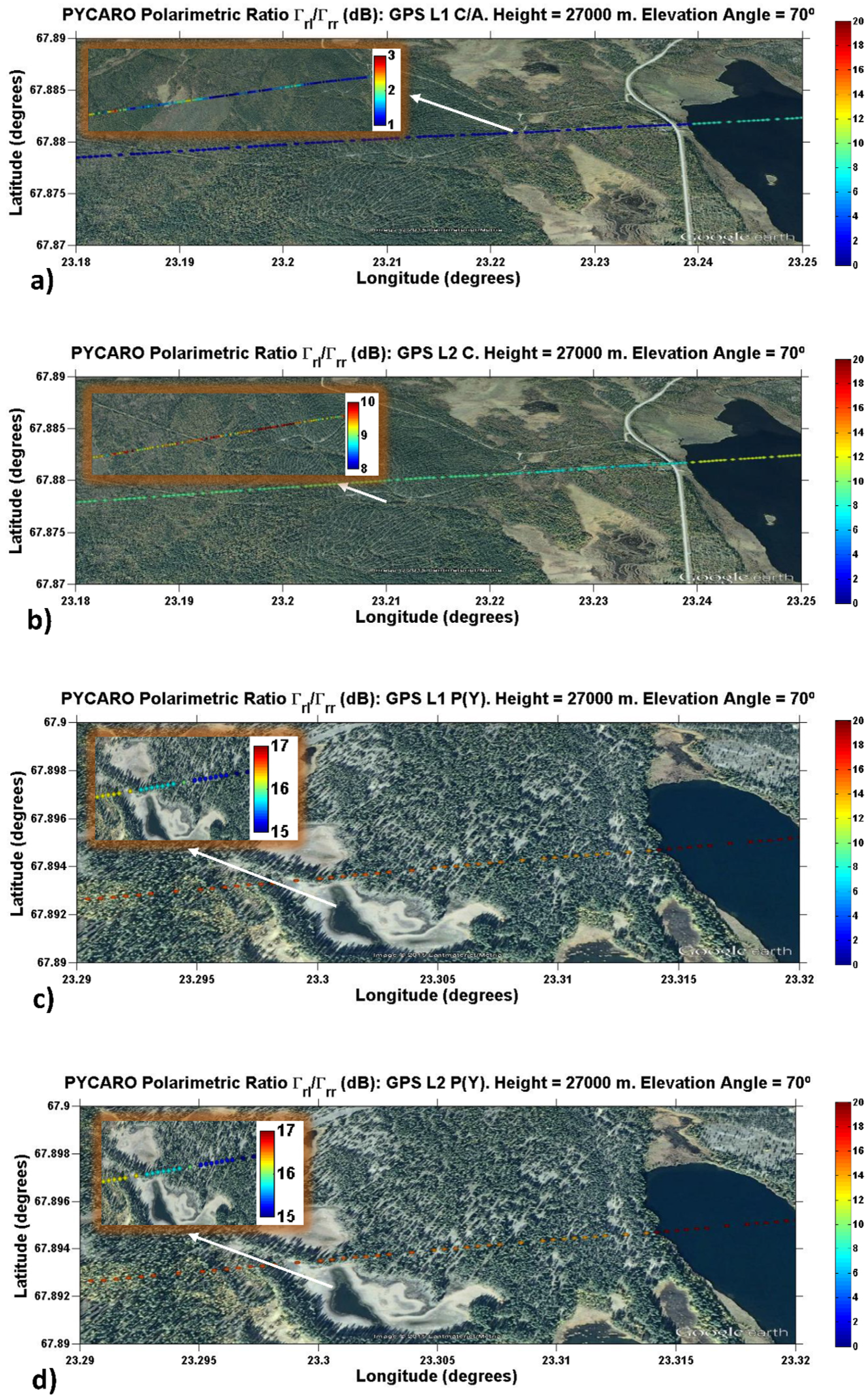
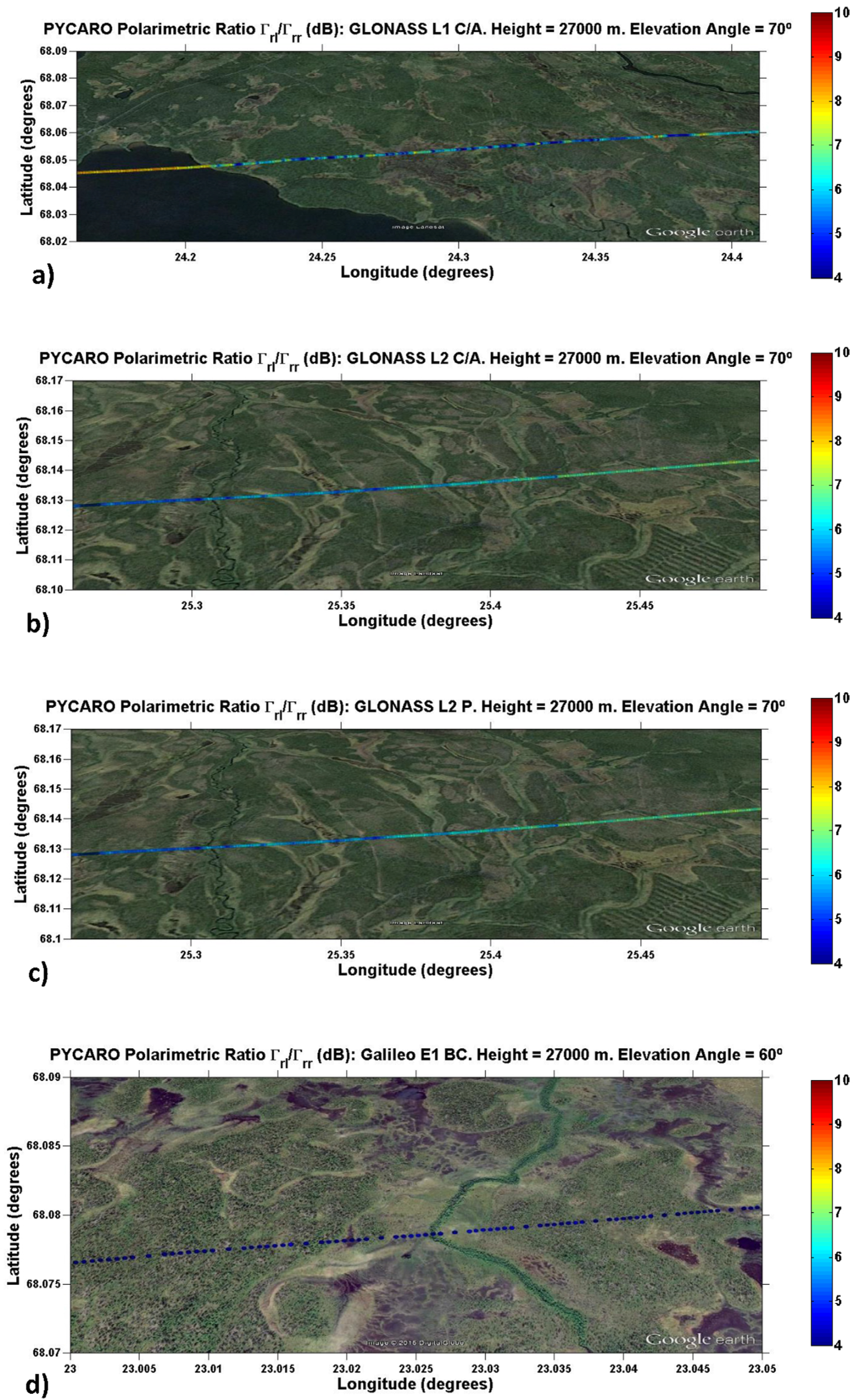
3. Results of a Stratospheric Balloon Experiment over Boreal Forests

The PYCARO reflectometer was operated in closed-loop mode during this experiment, with delay and phase tracking loops activated. It uses cGNSS-R technique to process the open-access codes, and the rGNSS-R one for the encrypted codes. The polarimetric study is performed using two different observables: the polarimetric ratio [15] and the polarimetric phase [22] using the measurements provided by the phase tracking loop. The polarization ratio is more sensitive to soil dielectric properties and can cancels roughness effects although it does not do so perfectly for arbitrary scattering media. It is defined as the ratio of the cross-over the co-polar reflectivities Γ rl / Γ rr , and it is estimated as the ratio of the peak of the reflected signal power waveform at LHCP | Y reflected , Peak l | 2 over the peak of the reflected signal power waveform at RHCP | Y reflected , Peak r | 2 , after proper compensation of the noise power floor and the antenna radiation pattern:
Γ rl Γ rr = | Y reflected , Peak l | 2 | Y reflected , Peak r | 2
where l and r denote Left and Right Hand Circular Polarization, respectively. Note that the noise power floor of the reflected waveforms | Y noise | 2 has to be subtracted to the reflected power waveform | Y | 2 to obtain the power of the signal itself | Y signal | 2 . Additionally, the different gain of the antenna array at LHCP (12.9 dB at L1-LHCP and 11.6 at L2-LHCP) and RHCP (13.3 dB at L1-RHCP and 11.6 dB at L2-RHCP) have to be compensated by subtracting the antenna gain to the reflected signal power. Once the effect of the noise and the antenna have been compensated, the incoherent power component is omitted in the reflectivity, as obtained using Equation (1), by subtracting to each incoherently averaged waveform’s peak | Y reflected , Peak | 2 the amplitude variance of the complex waveforms’ peaks σ | Y reflected , Peak | 2 [23]:
| Y reflected , Peak | 2 = | Y reflected , Peak | 2 σ | Y reflected , Peak | 2
Thus, reflectivity values are associated to the first Fresnel zone. The semi-major axis of the first Fresnel zone during the float phase of the flight and for an elevation angle θe = 70° is: GPS L1 Coarse/Acquisition C/A (74 m), GPS L2 Precise/Secure P(Y) (83 m), GPS L1 P(Y) (74 m), GPS L2 Civilian C (83 m), GLONASS L1 C/A (74 m), GLONASS L2 C/A (83 m), GLONASS L2 Precise P (83 m) and Galileo E1 BC (74 m). Additionally, the difference of the unwrapped phases of the complex waveforms peak at LHCP Ψ n l and RHCP Ψ n r can be used. This phase has two terms; one induced during the scattering process, which is roughly constant at high elevation angles (e.g., θe ≥ 60°), and another one due to the propagation. As compared to the polarimetric ratio the main advantage is that the phase difference between the RHCP and LHCP signals can be modeled independently of the elevation angle [22].
After compensation of the first term (using as a first approximation a flat soil model (e.g., Equations (18) and (19) in [24]) the phase difference δΨ n between the peak amplitude of the LHCP and the RHCP reflected complex waveforms at time tn can be used to infer the geometric delay difference ρ geo , n as:
ρ geo , n = λδΨ n 2 π
where λ is the signal wavelength. Height differences hn of the center of phase of the scatterers at LHCP and RHCP are related to the geometric delay difference ρ geo , n as:
h n = ρ geo , n 2 sinθ e
It is found that the mean of the polarimetric phase corresponding to GPS, GLONASS and Galileo signals over boreal forests is in the range from approximate −1.4 m to −9.6 m, which suggests that the phase center of the reflected signals at LHCP is higher than the one at RHCP, that is the scattering process takes place over the canopy and the soil [18]. The trajectory of the balloon was provided by Swedish Space Corporation (SSC) using a GPS receiver on-board, and small platform height variations were compensated for. Note that the vertical speed of the gondola during the float phase was smaller than 1 m/s, which prevented phase jumps. Single reflections (from RHCP to LHCP) are mainly due to interactions with the upper scatterers on the forests. On the other side, signals collected at RHCP involve multiple scattering soil–leaves and soil–branches (first from RHCP to LHCP and then from LHCP to RHCP). This is the reason that explains that the polarimetric phase has negative values (Equation (4)).
Figure 2 and Figure 3 show the first-ever maps of the polarimetric ratio using dual-band multi-constellation signals over boreal forests and lakes. The polarimetric ratio was provided over lakes and boreal forests to give a more complete information and description of the polarimetric properties in the GNSS-R case for different types of scattering media. In Figure 2 there are two different color scales to show a general overview of the polarimetric ratio and also the sensitivity of the technique over boreal forests as it can be seen in the embedded scales. For this study, the elevation angle of the selected satellites was θe = 70° for GPS and GLONASS, and θe = 60° for Galileo. This selection was made because for lower elevation angles the performance of the technique was degraded due to the high directivity of the down-looking antenna array. The maps correspond to different ground tracks. The polarimetric ratio values at the specular reflection points were geolocated and represented over the Earth’s surface using Google Maps for simpler interpretation. The ephemerides as provided by an on-board positioning receiver were used to derive the orbit parameters of the GNSS satellites, while the PYCARO trajectory was measured by the on-board receiver. cGNSS-R was used for data acquisition of GPS L1 C/A (Figure 2a), GPS L2 C (Figure 2b), GLONASS L1 C/A (Figure 3a), GLONASS L2 C/A (Figure 3b), GLONASS L2 P (Figure 3c) and Galileo E1 BC (Figure 3d) signals, while rGNSS-R for GPS L1 P(Y) (Figure 2c) and GPS L2 P(Y) (Figure 2d). The mean polarimetric ratio (PR) for GPS L1 C/A signals is ~8 dB and ~4.2 dB over lakes and boreal forests, respectively (Table 1). Additionally, it is found that for the so-called data-less signal GPS L2 C the ratio is, respectively, ~12.7 dB and ~8.1 dB over lakes and boreal forests. The reason that explains the higher values of PR of GPS L2 C as compared to GPS L1 C/A signals is that the depolarization of the direct signal (Table 2) is higher for L1 C/A than for L2 C signals SNR GPS , L 1 C / A , l = 13 dB and SNR GPS , L 2 C , l = 3 dB). The Signal-to-Noise Ratio (SNR) values of the direct signals are higher for L1 than for L2, as can be appreciated in Table 2. This is empirical evidence showing that the degree of depolarization is lower for GPS L2 C signals.
Figure 2. Measured polarimetric ratios for a flight height of 27,000 m and an elevation angle θe = 70° for (a) GPS L1 C/A, (b) GPS L2 C, (c) GPS L1 P (Y), (d) GPS L2 P (Y).
Remotesensing 07 13120 g002
The rGNSS-R is evaluated successfully for first time over forests, despite the large dispersion of the signal induced by the scattering media. The polarimetric ratio is larger as compared to the GPS L1 C/A signals, with a value ~20.4 dB and ~14.6 dB over lakes and boreal forests, respectively. It is worth pointing out some considerations about the squaring losses of the P (Y) code correlation technique implemented in PYCARO (rGNSS-R). They have a non-linear dependence with the SNR of the received signal [8]: The lower the SNR, the larger the squaring losses [25]. Therefore, the polarimetric ratio as derived from the P (Y) code is higher because of the SNR of the collected RHCP signals is lower than the LHCP ones. Additionally, the direct P (Y) signal depolarization is much lower as compared to the L1 C/A and the L2 C, which also contributes to a higher PR.
Figure 3. Measured polarimetric ratios for a flight height of 27,000 m and an elevation angle θe = 70° for (a) GLONASS L1 C/A, (b) GLONASS L2 C/A, (c) GLONASS L2 P; and for an elevation angle θe = 60° for (d) Galileo E1 BC.
Remotesensing 07 13120 g003
Maps of the mean polarimetric ratio for GLONASS L1 C/A (Figure 3a), L2 C/A (Figure 3b) and L2 P (Figure 3c) are also included. Values over lakes are found to be ~8.2 dB for GLONASS L1 C/A signals, in agreement with GPS L1 C/A signals (Table 1 and Table 2) because the corresponding direct signals have a similar level of depolarization, and the lakes scattering properties are the same independently of the track. On the other side, the effect of the different tracks (different forest structure) is manifested in the different values of the polarimetric ratio over forests because the signal depolarization due to the scattering, the propagation and the effect of multiple reflections. However, there were no signal acquisitions over lakes at RHCP for GLONASS L2 C/A and L2 P because the direct signal is found to be highly polarized (Table 2). Table 2 shows that there were no signal acquisitions of the direct GLONASS L2 C/A and L2 P signals at LHCP. This is an indication showing that these signals are highly polarized so that the SNR at LHCP is so low that could not be detected by the PYCARO instrument during the flight. On the other side, the following values are found over boreal forests: PR GLONASS , L 1 C / A ~ 6.7 dB, PR GLONASS , L 2 C / A ~ 6.3 dB and PR GLONASS , L 2 P ~ 6.3 dB.
Table 1. Mean polarimetric ratio over forests and lakes for GPS (L1 C/A, L2 C, L1 P (Y) and L2 P (Y)), GLONASS (L1 C/A, L2 C/A and L2 P) and Galileo (E1 BC) signals during the float phase of BEXUS 19 flight.
GNSS CodeElevation AnglePR (dB)
(Forests)
PR (dB)
(Lakes)
GPS L1 C/A θe ~ 70°4.28
GPS L2 P(Y) θe ~ 70°14.620.4
GPS L1 P(Y) θe ~ 70°14.620.4
GPS L2 C θe ~ 70°8.112.7
GLONASS L1 C/A θe ~ 70°6.78.2
GLONASS L2 C/A θe ~ 70°6.3-
GLONASS L2 P θe ~ 70°6.3-
Galileo E1 BC θe ~ 60°4.1-
Table 2. Signal-to-Noise Ratio at RHCP y LHCP of the direct GPS (L1 C/A, L2 C, L1 P (Y) and L2 P (Y)), GLONASS (L1 C/A, L2 C/A and L2 P) and Galileo (E1 BC) signals as function of the elevation angle during the float phase of BEXUS 19 flight.
GNSS CodeSNRr (dB)
θe~ 70°
SNRl (dB)
θe~ 70°
SNRr (dB)
θe~ 60°
SNRl (dB)
θe~ 60°
SNRr (dB)
θe~ 50°
SNRl (dB)
θe~ 50°
SNRr (dB)
θe~ 40°
SNRl (dB)
θe~ 40°
GPS L1 C/A3413332332233023
GPS L2 P(Y)19-16-13-10-
GPS L1 P(Y)19-16-13-10-
GPS L2 C283253238218
GLONASS L1 C/A3112311829252115
GLONASS L2 C/A16-16-20-20-
GLONASS L2 P12-12-16-16-
Galileo E1 BC15-14-13-11-
In this work, authors use the available ground truth data to interpret the results, but unfortunately there are no ground truth data for each track. The PR for GLONASS L2 C/A and L2 P are found to be equal over the same track because the direct signals were no depolarized (Table 2). Finally, it is found that the polarimetric ratio for Galileo E1 BC over boreal forests for a different track and time of signal acquisition is PR Galileo , E 1 BC ~ 4.1 dB.
A common characteristic for all the GNSS signals is that the polarimetric ratio is lower over boreal forests ( PR GPS , L 1 C / A ~ 4.2 dB, PR GPS , L 2 C ~ 8.1 dB, PR GPS , P ( Y ) ~ 14.6 dB, and PR GLONASS , L 1 C / A ~ 6.7 dB) than over lakes PR GPS , L 1 C / A ~ 8 dB, PR GPS , L 2 C ~ 12.7 dB, PR GPS , P ( Y ) ~ 20.4 dB, and PR GLONASS , L 1 C / A ~ 8.2 dB). In this scenario, in addition to depolarization effects due to scattering and propagation through the vegetation, multiple reflections involving canopy-soil and soil-canopy increase the amount of co-polar signals in the final scattered field reaching the receiver.

4. Final Discussions

The BEXUS 19 stratospheric balloon experiment with an apogee of ~27,000 m has provided a unique opportunity to study for first time the scattering of GNSS signals over boreal forests. Multi-constellation (GPS, GLONASS and Galileo) reflected signals were collected by the PYCARO instrument at dual-band (L1, L2) and dual-polarization (RHCP, LHCP). These measurements provide the first experimental evidence towards the further evaluation of GNSS-R for polarimetric applications. First results show a promising performance of the PYCARO instrument as the payload for the 3Cat-2 mission. The scientific evaluation of this dataset offers the opportunity to evaluate the feasibility of the GNSS-R to perform biomass monitoring, which is a key-factor for analyzing the carbon cycle. The main added value is the measurement of polarimetric signatures, which shows sensitivity over forests and lakes. Additionally, different data acquisition techniques have been used: cGNSS-R for the open-source codes and the novel rGNSS-R for the encrypted P(Y) GPS code. The scattering of the GNSS-R signals takes place over the soil and the canopy but also through multiple reflections involving canopy-soil and soil-branches interactions. This is an important issue that has to be considered to perform biomass monitoring, since the vegetation provides a scattered field additionally to the effect of the attenuation of the signals reflected over the soil. Future work should include a study of: (a) The potential advantages of the synergy between both data access techniques, and (b) scattering over different types of vegetated soils.

5. Conclusions

The polarimetric ratio and the mean polarimetric phase over boreal forests with a biomass density of ~2,500 trees/ha and for an elevation angle of θe = 70° for GPS and GLONASS and θe = 60° for Galileo vary in the ranges from approximate 2 to 16 dB and from approximate −1.4 to −9.6 m, respectively. This is due to the effect of different tracks, periods of signal acquisition, levels of depolarization of the direct signals and because of the squaring losses of the rGNSS-R. The polarimetric phase is found to be negative, which means that the center of phase of the reflected signals at LHCP is higher in the vertical profile of the forests as compared with RHCP signals. As the main conclusion, GNSS-R has been shown to have sensitivity to perform polarimetric measurements over lakes and boreal forests from a stratospheric balloon flight with an apogee of 27,000 m using dual-band multi-constellation signals.
Additionally, a theoretical investigation of the different contributions to the total reflectivity over boreal forests has been performed and it is included in the appendix. The evolution of the reflectivity as a function of the elevation angle over boreal forests using simulations of the cross- (reflected LHCP) and co-polar (reflected RHCP) scattered fields over soil and canopy, including canopy-soil interactions, for three different levels of biomass density (725 trees/ha, 150 trees/ha and 72 tress/ha) has been analyzed. The total reflectivity is dominated by that of the soil. The canopy (branches, leaves) reflectivity variations for larger density levels are found to have a dependence with the elevation angle, the polarization of the reflected signal and the scatterer type. Cross-polar canopy reflectivity increments are from approximate 10 to 20 dB for elevation angles in the range θe = (10°, 80°). On the other side, attenuation due to signal propagation through forests leads to lower reflectivity values over soil as lower is the elevation angle, independently of the polarization. However, the polarization is found to be an important parameter that determines the reflectivity levels of canopy-soil interactions. Increments of canopy-soil cross-polar reflectivity values have a similar trend than those corresponding to soil scattering. Nonetheless, for elevation angles larger than ~30°, the former scattering mechanism shows a higher increment of reflectivity as compared to scattering only over the soil. Additionally, it is found that leaves–soil co-polar reflectivity levels reduces from 10 dB to 0 dB for elevation angles in the range θe = (10°, 80°), while for branches–soil interactions is roughly constant around zero.

Acknowledgments

The authors would like to thanks Mrs. Pons and Khoe from the administration of the Department of Signal Theory and Communications (TSC) of the Universitat Politècnica de Catalunya-Barcelona Tech (UPC) and the REXUS/BEXUS (ESA, DLR, SNSB, SSC, and ZARM) team for their collaboration, help and advice during all the project. Special thanks to Dra. Natacha Callens (ESA) and Mr. Alexander Kinnaird (SSC) for their help during the flight campaign, and to Mr. Sylvain Vey (ESA) for his advice during the thermal analysis.
This project has received funding from the European Union’s Seventh Framework Programme for research, technological development and demonstration under grant agreement “European GNSS-R Environmental Monitoring” no FP7-607126-E-GEM (Online Available: http://www.e-gem.eu), and by the project “Aplicaciones avanzadas en radio ocultaciones y dispersometría utilizando señales GNSS y otras señales de oportunidad” of the Spanish Ministerio de Ciencia e Innovación (MICINN), Grant No AYA2011-29183-C02-01.

Author Contributions

Hugo Carreno-Luengo and Adriano Camps conceived and designed the experiment; Hugo Carreno-Luengo performed the experiment; Hugo Carreno-Luengo analyzed the data; Hugo Carreno-Luengo performed the theoretical simulations; Hugo Carreno-Luengo wrote the paper.

Appendix

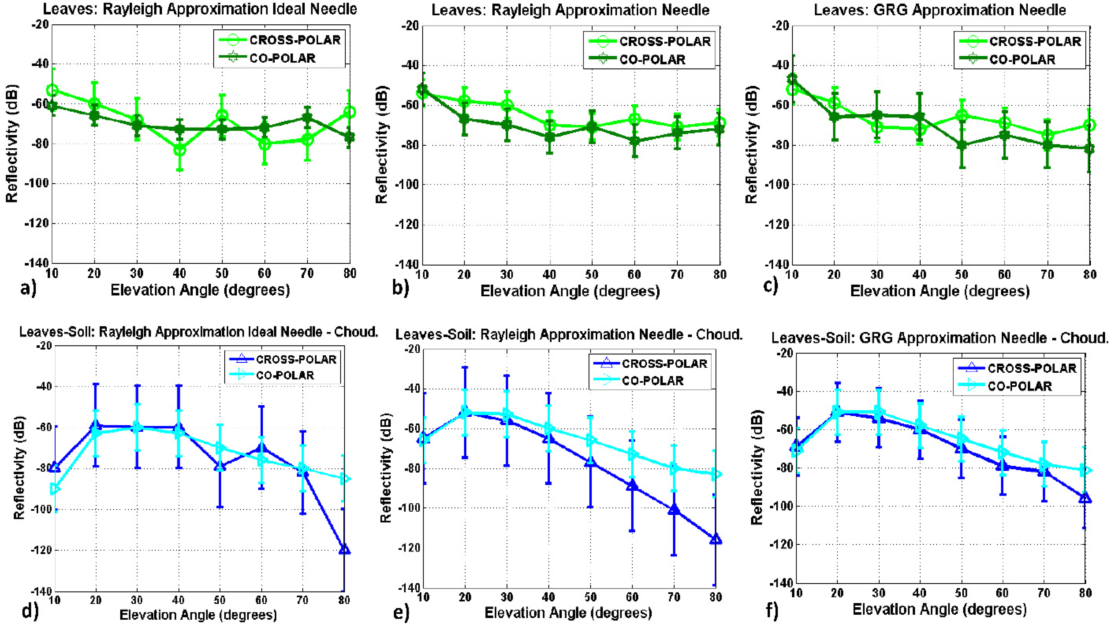
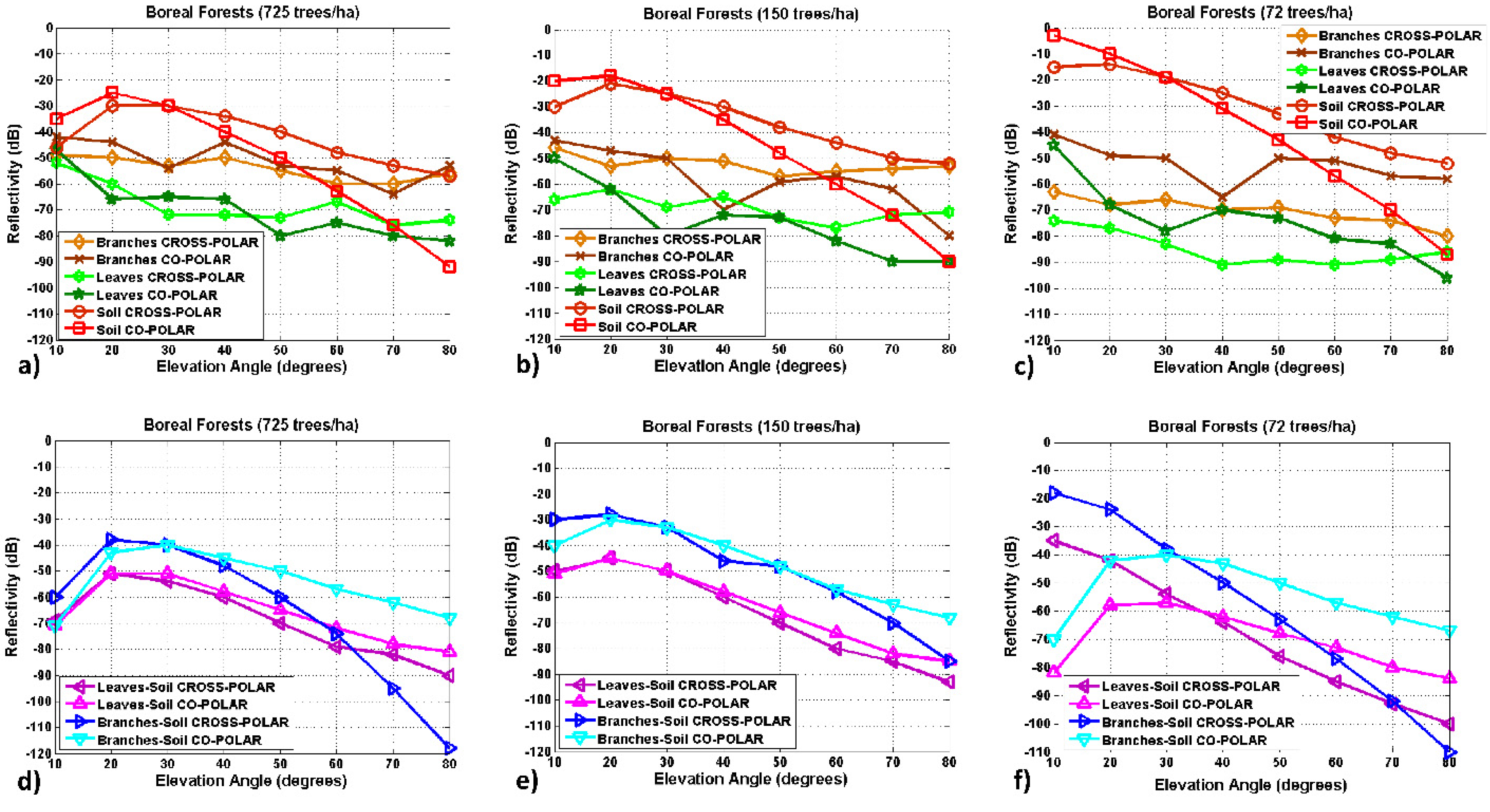
Part I: Simulations of the Reflectivity over Boreal Forests

Part I of the appendix provides a theoretical analysis of the reflectivity over boreal forests. The bistatic geometry of GNSS-R is represented in Figure A1a, and a sample 3-D structure of the tree type used in the simulations is represented in Figure A1b. Simulations of the reflectivity at L1-band over forests have been performed with a modified version of EMISVEG (appendix Part II) using signals at Right Hand Circular Polarization (RHCP) and Left Hand Circular Polarization (LHCP). In the considered scattering model, individual tree components located above a tilted dielectric rough plane are illuminated by the electromagnetic field and the scattered fields are computed, and then added coherently, as in [26]. Branches and tree trunks are modeled by stratified dielectric cylinders, arranged following a fractal geometry described by Lindenmayer systems [27]. The leaves are modeled by dielectric needles, and are added to the tree model. This scattering model preserves the phase of scattering fields from scatterers (leaves, branches, and trunks) in the simulation of this coherent signature from the forest. The effect of attenuation and phase change of the coherent wave propagating in the forest media is also taken into account using the Foldy’s approximation [28].
The scattering matrix S = was transformed from linear to circular polarization. This matrix relates the components of the scattered field E ¯ s and the incident field E ¯ i for all the polarimetric combinations:
[ E r s E l s ] = e jkR 0 R 0 [ S rr S rl S lr S ll ] [ E r i E l i ]
where R 0 is the distance from the specular point to the receiver, which is a function of the scatterer. Subscripts r and l denote Right Hand Circular Polarization and Left Hand Circular Polarization, respectively.
These simulations provide reflectivity values for the soil, branches (tree trunks are also included into the simulations), leaves and multiple reflections involving leaves-soil and branches-soil interactions, as in [18]. EMISVEG was originally developed for full-polarimetric microwave emission studies at L-band, but it has been now adapted to compute the forward scattering. L-band (1.400–1.427 MHz) data from the SMOS REFLEX 2004 field experiment [29] were used to validate the model. In the frame of this work, it has been modified to evaluate the forward scattering coefficient over boreal forests at circular polarization using the Forward Scattering Alignment (FSA) convention.
Figure A1. (a) Reference system following the Forward Scattering Alignment (FSA) criterion. (b) Sample 3-D structure of the tree-type used along the simulations performed to estimate the reflectivity.
Remotesensing 07 13120 g004
Figure A2. Simulated reflectivity for a biomass density of 725 tress/ha over leaves: (a) Rayleigh approximation ideal needle, (b) Rayleigh approximation needle, (c) Generalized Rayleigh Gans approximation needle; and leaves-soil interactions: (d) Rayleigh approximation ideal needle-Choudhury, (e) Rayleigh approximation needle-Choudhury, and (f) Generalized Rayleigh Gans approximation needle-Choudhury.
Remotesensing 07 13120 g005
The vegetation height was set to be ~20 m (Figure A1b) based on the available ground truth data [30,31], and the scattering area was set to be equal to the first Fresnel zone A Fresnel . The attenuation coefficient over canopy at L band is ~1.5 dB/m. A much lower tree density for a biomass density of 100 t/ha (725 trees/ha instead ~2,700 trees/ha as in [32] for a tree height ~20 m) was required to make the simulations feasible. The electromagnetic models selected for the expression of the bistatic scattering matrices were the Semi-Exact solution for the branches S = branches [33], the Generalized Rayleigh-Gans (GRG) approximation for a needle in the case of leaves S = needle [34], and the Choudhury method for the soil S = soil [35]. The Semi-Exact solution was selected because the radii of curvature of the branches of Northern Sweden forests is not an order of magnitude larger than the signals wavelength used in the simulations λ L 1 = 19 cm). The Physical Optics approximation for higher frequencies provides a fast algorithm when the radius of tree branches is large compared to the wavelength [33]. The GRG approximation for a needle was selected to evaluate the scattering on leaves because: (a) Needles are the best geometrical approximation for leaves in coniferous vegetation, and (b) GRG is valid for a scatterer with at least one of its dimensions small as compared to the signals wavelength [34]. Nonetheless, several simulations were performed to evaluate the differences with other methods: Rayleigh approximation for an ideal needle (Figure A2a), Rayleigh approximation for a needle (Figure A2b), and the GRG approximation for a needle (Figure A2c). Additionally, the leaves–soil scattering mechanism was evaluated using the same scattering methods for the leaves, and the Choudhury method [35] to account for the electromagnetic interaction with the soil (Figures A2d–f). These simulations show that there are several differences: (a) A larger dynamic range of the co-polar reflectivity over leaves using the GRG method (~30 dB) as compared to that obtained with the Rayleigh approximation for an ideal needle (~20 dB); and (b) both the cross- and the co-polar reflectivities for leaves–soil interactions.
The cross-polar values are under-estimated as compared to the GRG-Choudhury method (from ~10 dB at low elevation angles θe ~ 10°, to ~20 dB for high elevation angles, θe ~ 80°). On the other side, the co-polar reflectivity levels are under-estimated ~20 dB using the Rayleigh approximation for an ideal needle for low elevation angles, θe ~ 10°.
After these previous considerations, the cross- and co-polar reflectivity coefficients are analyzed as a function of the elevation angle in the range θe = (10°, 80°) for three different biomass densities 725 trees/ha (Figure A3a, single reflections; and Figure A3d, multiple reflections), 150 trees/ha (Figure A3b, single reflections; and Figure A3e, multiple reflections) and 72 trees/ha (Figure A3c, single reflections; and Figure A3f, multiple reflections). The co-polar component over soil-surface is dominant for low elevation angles up to θe ~ 30°, while the cross-polar is the highest component for larger elevation angles. Actually, this corresponds to the Brewster angle, which is a property of the reflector type and indicates the change of polarity of the vertical component of incident electromagnetic field after being reflected [36]. A common characteristic of the full ranges of biomass densities and elevation angles under study is the order of reflectivity levels. First of all, the soil surface (on average ~10 dB more than other contributions), which is followed by reflectivity levels over branches and leaves.
Figure A3. Cross- and co-polar reflectivity simulations over forests: (ac) direct scattering (canopy, soil) and (df) multiple scattering (canopy–soil interactions), for a biomass density of (a,d) 725 trees/ha, (b,e) 150 trees/ha, and (c,f) 72 trees/ha.
Remotesensing 07 13120 g006
The study of multiple reflections involving both leaves-soil and soil-leaves, and both branches-soil and soil-branches shows that the cross-polar component is the highest for low elevation angles up to θe ~ 30°, while the co-polar one is the highest component for higher elevation angles. This inversed-behavior as compared with single reflections is due the double polarization changes induced by, first from RHCP to LHCP, and then from LHCP to RHCP.

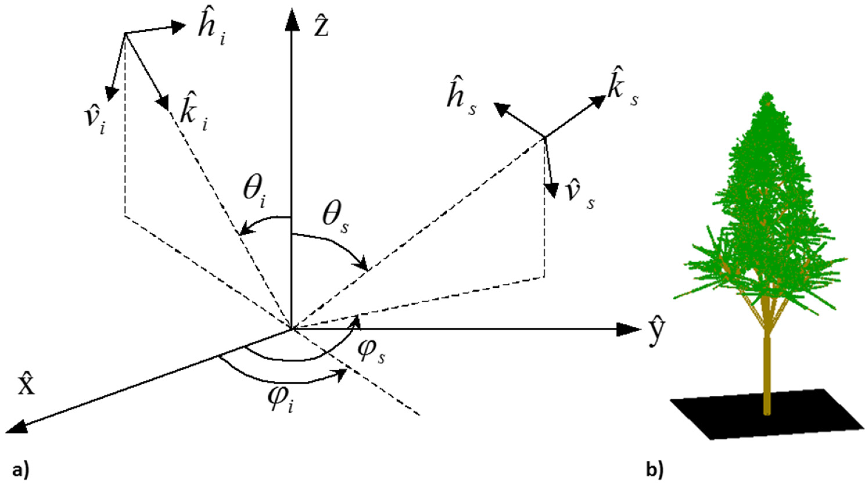
Part II: Theoretical Electromagnetic Model

The presented model has to be validated and it represents a theoretical investigation of the different contributions to total reflectivity. The model should satisfy the following premises to properly simulate the properties of GNSS reflectometry during the experiment using the PYCARO instrument: (a) Realistic 3-D spatial structure of a forest, in which every scatterer has its deterministic location; (b) accurate generation of tree structures based on physical parameters; (c) account for the coherent effects that may exist in different scatterers; (d) account for the scattering contribution from the scatterers in the forest canopy, and also for the direct scattering of the rough ground surface; (e) the scattered fields of adjacent trees in a forest stand are assumed to be uncorrelated; (f) the effect of attenuation and phase change of the coherent wave propagating in the random media; and (g) only the scattering in the forward direction has to be accounted for.
The total scattered field within the first Fresnel zone can be written as a function of the position of the nominal specular point ρ ¯ as follows:
E ¯ s ( ρ ¯ ( t ) ) = E ¯ soil s ( ρ ¯ ( t ) ) + E ¯ forest s , leaves ( ρ ¯ ( t ) ) + E ¯ forest s , leaves _ soil ( ρ ¯ ( t ) ) + E ¯ forest s , soil _ leaves ( ρ ¯ ( t ) ) + E ¯ forest s , branches ( ρ ¯ ( t ) ) + E ¯ forest s , branches _ soil ( ρ ¯ ( t ) ) + E ¯ forest s , soil _ branches ( ρ ¯ ( t ) )
where E ¯ soil s , E ¯ forest s , leaves , E ¯ forest s , leaves _ soil , E ¯ forest s , soil _ leaves , E ¯ forest s , branches , E ¯ forest s , branches _ soil , and E ¯ forest s , soil _ branches are the total forward scattered fields by soil surface, leaves, multiple interactions involving both soil and leaves, branches, and multiple interactions involving branches and soil, respectively. Since the specular reflection point changes with time, the values of the electric fields in Equation (A2) are also a function of time.The Choudhury method [35] is used to simulate the direct scattering of the GPS signals E ¯ soil s over the ground surface. To the first order of approximation, the scattering from every type of forest element is approximated by the superposition of the scattered field from each scatterer within the tree structure. Hence, neglecting the effect of multiple scattering among the scatterers, the scattered field from a single tree for every type of forest element can be evaluated by [26]:
E ¯ s , element = e jkr r n = 1 N e j ϕ n S = n interaction E ¯ 0 i , element
where j = 1 is the imaginary unit, N is the total number of the scatterers within the tree structure, S = n interaction is the scattering matrix in circular polarization of the nth scatterer above the soil corresponding to a forest element, ϕ n is a phase compensation term accounting for the shift of the phase reference from the local coordinate system of the nth scatterer to the global coordinate phase reference, and E ¯ 0 i , element is the amplitude of the incident electromagnetic wave. Denoting the position of the nth scatterer in the global coordinate system by r ¯ n , ϕ n is given by [26]:
ϕ n = ( k ¯ i k ¯ s ) r ¯ n
where k ¯ i and k ¯ s are, respectively, the unit vectors representing the propagation direction of the incident and the scattered fields.
The forest element scattered field E ¯ forest s , element is modeled taking into account the effect of attenuation and phase change of the coherent wave E ¯ s , element propagating in the random media (boreal forest). Based on Foldy’s approximation [28], the variation of the mean field E ¯ forest s , element with respect to the distance s along the direction k ¯ is generally governed by:
d E ¯ forest s , element ds = jK E ¯ forest s , element
where K is the effective propagation constant. Using eigen-analysis, the differential Equation (A5) is solved and the solution is given by:
E ¯ forest s , element = e jk o s T = ( s , k ¯ ) E ¯ forest s , element , 0
where T = is the transmissivity matrix accounting for the extinction due to scattering and absorption, and E ¯ forest s , element , 0 is the forest scattered field at s = 0 .
To account for this last term and for the bistatic nature of the GNSS reflectometry, the expressions for the scattering matrix as proposed in [26] in the forward-scatter direction of each different forest element interactions S = n interaction are modeled as follows:
S = n element = T = n i S = n 0 ( k ¯ s , k ¯ i ) T = n i
S = n element , soil = e n T = t R = ( k ¯ s , k ¯ gs ) T = n r S = n 0 ( k ¯ gs , k ¯ i ) T = n i
S = n soil , element = e n T = n i S = n 0 ( k ¯ s , k ¯ gi )   T = n r R = ( k ¯ gi , k ¯ i ) T = t
where S = n element , S = n element , soil , and S = n soil , element are the direct scattering, the element-soil scattering and the soil-element scattering matrices, respectively. T = n i , T = n r , and T = t are the transmissivity matrices, respectively, for the direct, reflected, and total travelling path, and R = is the reflection matrix of the rough tilted ground plane whose elements are derived as per Wang and Choudhury [37], and:
k ¯ gi = k ¯ i 2 n ¯ g ( n ¯ g k ¯ i )
k ¯ gs = k ¯ s 2 n ¯ g ( n ¯ g k ¯ s )
τ i = 2 k 0 ( n ¯ n n ¯ g ) ( n g k ¯ i )
τ s = 2 k 0 ( n ¯ n n ¯ g ) ( n ¯ g k ¯ s )
where the phase terms τi and τs account for the extra path lengths of the image excitation and the image scattered waves, respectively, and k ¯ i , k ¯ s , k ¯ gi , k ¯ gs and n ¯ g are defined in Figure A4.
The electromagnetic models selected for the expression of the bistatic scattering matrices S = n 0 are the Semiexact solution for the branches [33], and the Generalized Rayleigh-Gans approximation for a needle in the case of leaves [34].
The incident L1 GPS signals after the scattering over the ground surface ((a) in white in Figure A4a) are collected by the receiver. The direct scattering over the canopy attenuates and scatters forward the incident GPS signals without reaching the trunks. The incident GPS wavefront is first scattered by the canopy ((b) in white in Figure A4b). There is a component in the specular direction, but also, a fraction of it penetrates the trunks, reaches the ground ((c) in white in Figure A4c) and is reflected on the ground, and travels up through the upper layers to the receiver ((d) in white in Figure A4c). As a complement of the latter contribution, ground reflection ((e) in white in Figure A4c) followed by specular scattering over the canopy ((f) in white in Figure A4c) is also considered. The incident wave propagates through the upper layers and is attenuated by them before it scatters over the ground. The upward reflected GPS signals penetrate the trunks and are scattered by the canopy. As the last contribution, specular scattering on the trunks ((g) in white in Figure A4d) followed by ground reflection ((h) in white in Figure A4d) is considered. This mechanism is similar to the canopy–soil one. However, the scattering process occurs in the trunks instead of the canopy, and the canopy acts as an attenuating medium. Ground reflection ((i) in white in Figure A4d) followed by trunk specular scattering ((j) in white in Figure A4d) complements the latter mechanism, being similar to the soil–canopy mechanism.
Figure A4. (a) Soil scattering. (b) Direct scattering over canopy. (c) Multiple scattering involving soil and canopy. (d) Multiple scattering involving both soil and branches.
Remotesensing 07 13120 g007
The statistics of the scattered field are approximated from a Monte-Carlo simulation in which a large number of tree structures are generated using stochastic L-systems [38] and then the scattering matrix of all generated trees are computed. The total forest element scattered field in circular polarization E ¯ forest s , element is obtained as the mean of 100 Monte-Carlo realizations to average the position of the scatterers. A large number of fractal-generated trees (725, 150 and 72 trees/ha) is considered during the Monte-Carlo simulations to characterize the statistics of the scattered signals. Finally, the reflectivity is defined as [39]:
Γ = 1 4 πsinθ e i σ 0 s = 1 4 πsinθ e i | E ¯ s | 2 / A | E ¯ i | 2 / 4 πR 0 2 cosθ e s s e s
where θ e i is the elevation angle of the incident wave, θ e s and φ s are the elevation and azimuth angles of the scattered wave, and σ 0 is the forward scattering coefficient, A is the illuminated area, and the integration is carried out over the upper half space. Since around the direction of specular reflection the coherent component is much larger than the incoherent one, the integrand in Equation (A14) tends to a delta function. This allows reducing the integration limits around the specular direction. In our case, after inspection of the integrand, it was concluded that the contributions beyond a 4° × 4° domain had a negligible contribution to the computed reflectivity value.

Conflicts of Interest

The authors declare no conflict of interest.

References

  1. Martín-Neira, M. A PAssive Reflectometry and Interferometry System (PARIS): Application to ocean altimetry. ESA J. 1993, 17, 331–355. [Google Scholar]
  2. Garrison, J.L.; Katzberg, S.J.; Hill, M.I. Effect of sea roughness on bistatically scattered range coded signals from the global positioning system. Geophys. Res. Lett. 1998, 25, 2257–2260. [Google Scholar] [CrossRef]
  3. Fabra, F. GNSS-R as A Source of Opportunity for Remote Sensing of the Cryosphere. Ph.D. Thesis, Universitat Politècnica de Catalunya, Barcelona, Spain, 2014. [Google Scholar]
  4. Rodriguez-Alvarez, N. Contributions to Earth Observation Using GNSS-R Opportunity Signals. Ph.D. Thesis, Universitat Politècnica de Catalunya, Barcelona, Spain, 2011. [Google Scholar]
  5. Zavorotny, V.U.; Gleason, S.; Cardellach, E.; Camps, A. Tutorial on remote sensing using GNSS bistatic radar of opportunity. IEEE Geosci. Remote Sens. Mag. 2014, 2, 8–45. [Google Scholar] [CrossRef]
  6. Garrison, J.L.; Komjathy, A.; Zavorotny, V.; Katzberg, S.J. Wind speed measurement using forward scattered GPS signals. IEEE Trans. Geosci. Remote Sens. 2002, 40, 50–65. [Google Scholar] [CrossRef]
  7. Cardellach, E.; Rius, A.; Martín-Neira, M.; Fabra, F.; Ribó, S.; Kainulainen, J.; Camps, A.; D’Addio, S. Consolidating the precision of interferometric GNSS-R ocean altimetry using airborne experimental data. IEEE Trans. Geosci. Remote Sens. 2014, 52, 4992–5004. [Google Scholar] [CrossRef]
  8. Carreno-Luengo, H.; Camps, A.; Ramos-Pérez, I.; Rius, A. Experimental evaluation of GNSS-reflectometry altimetric precision using the P (Y) and C/A signals. IEEE Sel. Top. Appl. Earth Obs. Remote Sens. 2014, 7, 1493–1500. [Google Scholar] [CrossRef]
  9. Unwin, M.; Jales, P.; Curiel, A.S.; Brenchley, M.; Sweeting, M.; Gommenginger, C.; Roselló, J. Sea state determination with GNSS reflectometry on TechDemoSat-1. In Proceedings of the 2014 ESA Small Satellites, Systems and Services Symposium, Mallorca, Spain, 26–30 May 2014.
  10. Unwin, M. TechDemoSat-1 and the GNSS reflectometry experiment. Available online http://www.merrbys.co.uk:8080/CatalogueData/Documents/TDS-1%20SGR-ReSI%20Experiment.pdf (accessed on 5 June 2015).
  11. Rose, R.; Wells, W.; Rose, D.; Ruf, C.; Ridley, A.; Nave, K. Nanosat technology and managed risk: An update of the CYGNSS microsatellite constellation mission development. In Proceedings of the 28th AIAA/USU Conference on Small Satellites, Logan, UT, USA, 4–7 August 2014; pp. 1–12.
  12. Wickert, J.; Beyerle, G.; Cardellach, E.; Förste, C.; Gruber, T.; Helm, A.; Hess, M.P.; Hoeg, P.; Jakowski, N.; Kern, M.; et al. GEROS-ISS-GNSS rEflectometry, Radio Occultation and Scatterometry on-board the International Space Station. In Proceedings of 4th International Colloquium Scientific and Fundamental Aspects of the Galileo Programme, Espoo, Finland, 28–31 October 2013.
  13. Martín-Neira, M.; D’Addio, S.; Buck, C.; Floury, N.; Prieto-Cerdeira, R. The PARIS ocean altimeter in-orbit demonstrator. IEEE Trans. Geosci. Remote Sens. 2011, 49, 2209–2237. [Google Scholar] [CrossRef]
  14. Carreno-Luengo, H.; Camps, A.; Jové, R.; Alonso, A.; Olivé, R.; Amèzaga, A.; Vidal, D.; Munoz, J.F. The 3Cat-2 project: GNSS-R In-Orbit demonstrator for earth observation. In Proceedings of the 2014 ESA Small Satellites, Systems and Services Symposium, Mallorca, Spain, 26–30 May 2014.
  15. Zavorotny, V.U.; Voronovich, A.G. Bistatic GPS signal reflections at various polarizations from rough land surface with moisture content. In Proceedings of the 2000 IEEE International Geoscience and Remote Sensing Symposium, Honolulu, Hawaii, USA, 24–28 July 2000; pp. 2852–2854.
  16. Ferrazzoli, P.; Guerriero, L.; Pierdicca, N.; Rahmoune, R. Forest biomass monitoring with GNSS-R: Theoretical simulations. Adv. Space Res. 2011, 47, 1823–1832. [Google Scholar] [CrossRef]
  17. Egido, A.; Paloscia, S.; Motte, E.; Guerriero, L.; Pierdicca, N.; Caparrini, M.; Santi, E.; Fontanelli, G.; Floury, N. Airborne GNSS-R soil moisture and above ground biomass observations. IEEE Sel. Top. Appl. Earth Obs. Remote Sens. 2014, 7, 1522–1532. [Google Scholar] [CrossRef]
  18. Wu, X.R.; Jin, S.G. GPS-Reflectometry: Forest canopies polarization scattering properties and modelling. Adv. Space Res. 2014, 54, 863–870. [Google Scholar] [CrossRef]
  19. Martínez-Vazquez, A. Emisividad Polarimétrica del Terreno Efecto de la Vegetación. Master’s Thesis, Universitat Politècnica de Catalunya, Barcelona, Spain, 2001. [Google Scholar]
  20. Ledesma-Galera, I. Estudio Experimental del Comportamiento Radiométrico de LAS Superfícies naturales. Master’s Thesis, Universitat Politècnica de Catalunya, Barcelona, Spain, 2002. [Google Scholar]
  21. Kinnaird, A. BEXUS User Manual. Available online: http://www.rexusbexus.net/index.php?option=com_content&view=article&id=51&Itemid=63 (accessed on 5 December 2014).
  22. Cardellach, E.; Ribó, S.; Rius, A. Technical Note on Polarimetric Phase Interferometry (POPI). Available online: http://arxiv.org/pdf/physics/0606099.pdf (accessed on 1 March 2015).
  23. Beckmann, P.; Spizzichino, A. The Scattering of Electromagnetic Waves from Rough Surfaces; Artech House Inc.: Norwood, MA, USA, 1963; p. 125. [Google Scholar]
  24. Smyrnaios, M.; Schon, S. Multipath Propagation, Characterization and Modelling in GNSS. Available online: http://cdn.intechopen.com/pdfs-wm/43710.pdf (accessed on 9 September 2015).
  25. Woo, T.K. Optimum semi-codeless carrier phase tracking of L2. In Proceedings the 12th International Technical Meeting of the Satellite Division of the Institute of Navigation, Nashville, TN, USA, 14–17 September 1999; pp. 82–99.
  26. Yi-Cheng, L.; Sarabandi, K. A Monte Carlo coherent scattering model for forest canopies using fractal-generated trees. IEEE Trans. Geosci. Remote Sens. 1999, 37, 440–451. [Google Scholar] [CrossRef]
  27. Prusinkiewicz, P.; Lindenmayer, A. The Algorithmic Beauty of Plants; Springer-Verlag: New York, NY, USA, 1990. [Google Scholar]
  28. Tsang, L.; Kong, J.A.; Shin, R.T. Theory of Microwave Remote Sensing; Wiley Interscience: New York, NY, USA, 1985. [Google Scholar]
  29. Martínez-Vazquez, I.; Camps, A.; Lopez-Sanchez, J.M.; Vall-llosera, M.; Monerris, A. Numerical simulation of the full-polarimetric emissivity of vines and comparison with experimental data. Remote Sens. 2009, 1, 300–317. [Google Scholar] [CrossRef] [Green Version]
  30. Caicoya, A.T.; Kugler, F.; Hajnsek, I.; Papathanassiou, K. Boreal forest biomass classification with TANDEM-X. In Proceedings of the 2012 IEEE International Geoscience and Remote Sensing Symposium, Munich, Germany, 22–27 July 2012; pp. 3439–3442.
  31. Global map of forest height produced from NASA’s ICESAT/GLAS, MODIS and TRMM sensors. Available online: http://www.nasa.gov/topics/earth/features/earth20120217map.html (accessed on 1 March 2015).
  32. Imhoff, M.L. Radar backscattering and biomass saturation: Ramifications for global biomass inventory. IEEE Trans. Geosci. Remote Sens. 1995, 33, 511–518. [Google Scholar] [CrossRef]
  33. Lin, Y.-C.; Sarabandi, K. Electromagnetic scattering model for a tree trunk above a tilted ground plane. IEEE Trans. Geosci. Remote Sens. 1995, 33, 1063–170. [Google Scholar]
  34. Karam, M.A.; Fung, A.K.; Antar, Y.M.M. Electromagnetic wave scattering from some vegetation samples. IEEE Trans. Geosci. Remote Sens. 1998, 26, 799–808. [Google Scholar] [CrossRef]
  35. Choudhury, B.J.; Schmugge, T.J.; Chang, A.; Newton, R.W. Effect of surface roughness on the microwave emission from soils. J. Geophys. Res. 1979, 84, 5699–5706. [Google Scholar] [CrossRef]
  36. Rodriguez-Alvarez, N.; Camps, A.; Vall-llosera, M.; Bosch-Lluis, X.; Monerris, A.; Ramos-Pérez, I.; Valencia, E.; Marchán-Hernandez, J.F.; Martinez-Fernandez, J.; Baroncini-Turricchia, G.; et al. Land geophysical parameters retrieval using the interference pattern GNSS-R technique. IEEE Trans. Geosci. Remote Sens. 2011, 49, 71–84. [Google Scholar] [CrossRef]
  37. Ulaby, F.T.; Moore, R.K.; Fung, A.K. Radar remote sensing and surface scattering and emission theory. In Microwave Remote Sensing: Active and Passive; Addison-Wesley: Reading, MA, USA, 1982; Volume II, pp. 1540–1541. [Google Scholar]
  38. Lindermayer, A. Developmental algorithms for multicellular organisms: A survey of L-systems. J. Theor. Bio. 1975, 54, 3–22. [Google Scholar] [CrossRef]
  39. Ulaby, F.T.; Moore, R.K.; Fung, A.K. Microwave remote sensing fundamentals and radiometry. In Microwave Remote Sensing: Active and Passive; Addison-Wesley: Reading, MA, USA, 1982; Volume I, pp. 249–251. [Google Scholar]

