A Spectral Decomposition Algorithm for Estimating Chlorophyll-a Concentrations in Lake Taihu, China


Abstract
:
1. Introduction
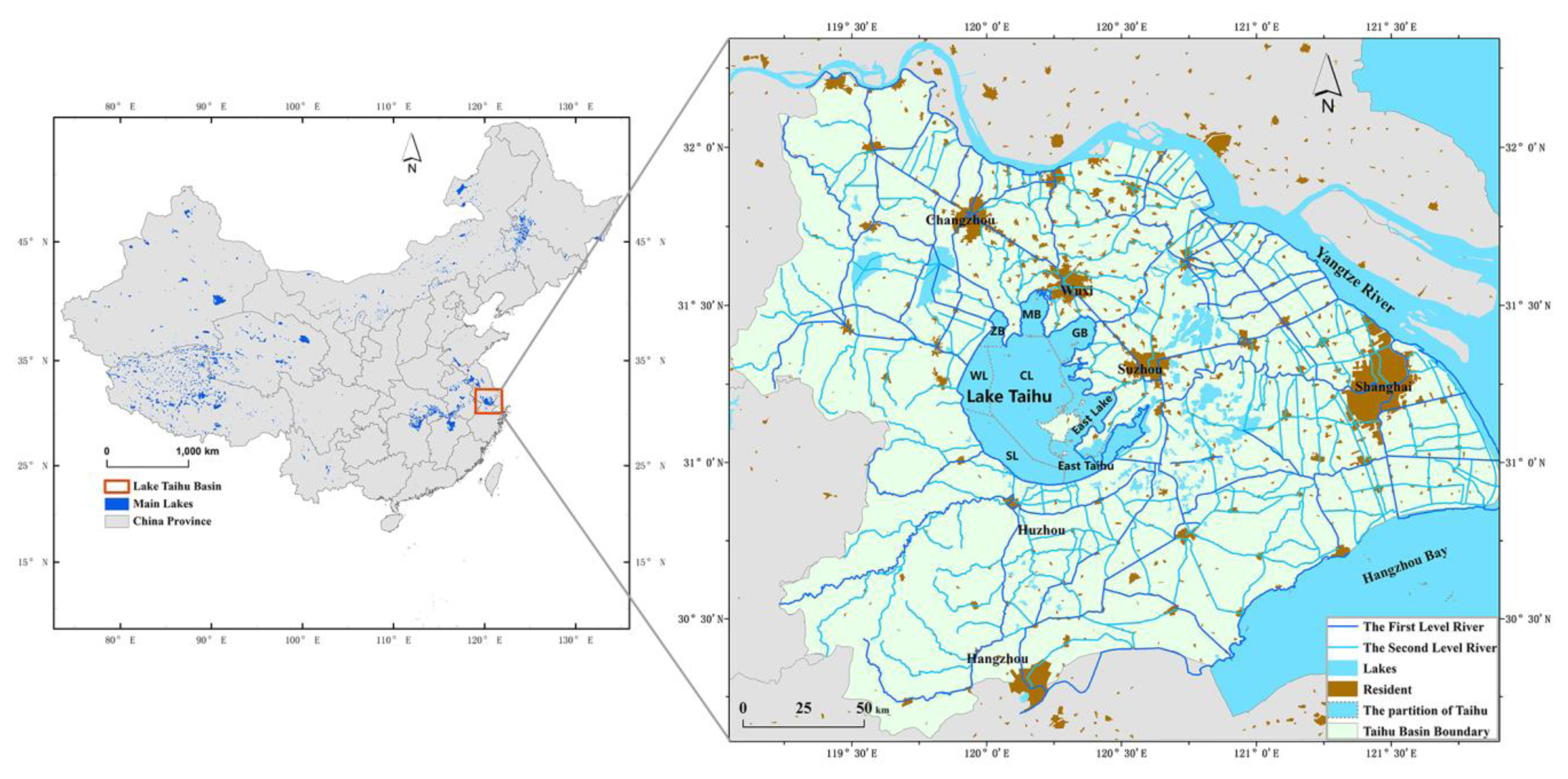
2. Study Area
3. Materials
3.1. Simulated Dataset
- Inherent optical property (IOP) specification model: CASE2;
- Pure water IOP [39];
- IOP specifications for Chla, NPSS and CDOM including a concentration profile, specific absorption and specific scattering spectra [26];
- Internal Source and Inelastic Scatter Selection linked to Chlorophyll Fluorescence, CDOM Fluorescence and Raman Scattering;
- Wind speed of 3.5 m/s (average of wind speed in Lake Taihu) and solar zenith angle of 30°;
- Parameters of air-water surface boundary conditions, sky conditions and bottom boundary condition were set to their default values.
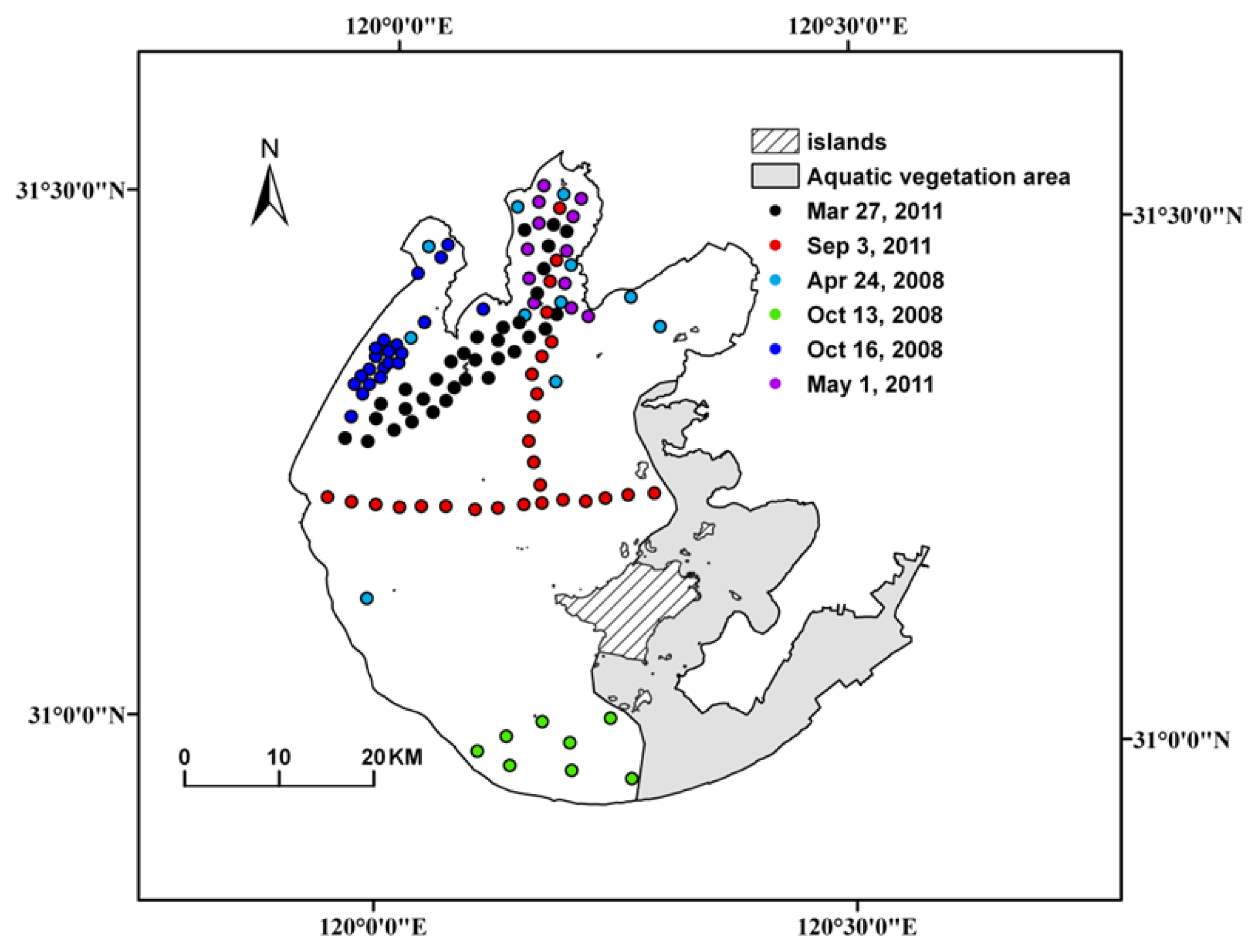
3.2. Field Measurements
3.3. MERIS Images
4. Methods
4.1. The Spectral Decomposition Algorithm for Lake Taihu
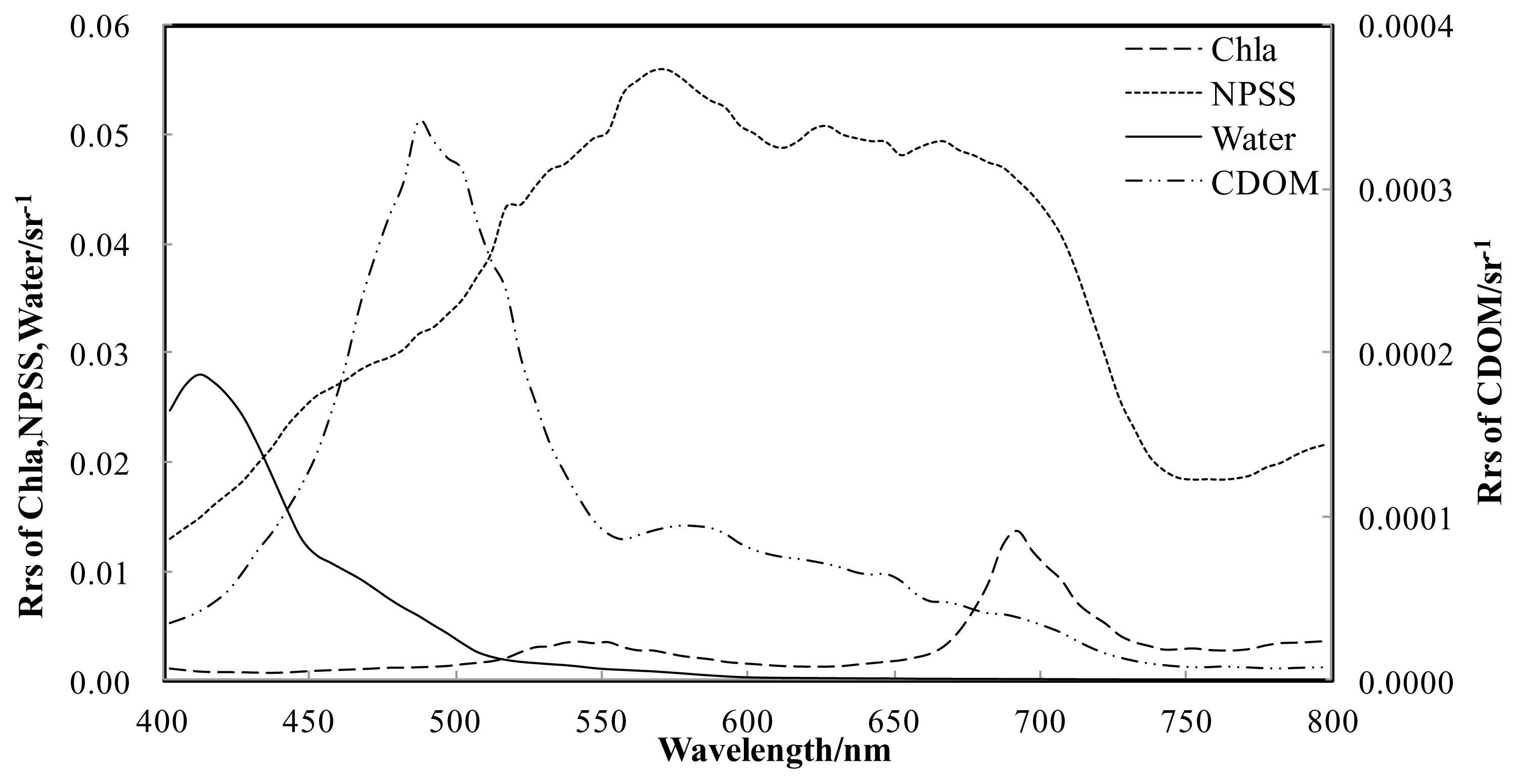
4.2. The Spectral Properties of End-Members
5. Results
6. Validation
7. Discussions
7.1. Accuracy Estimation Using MERIS Data
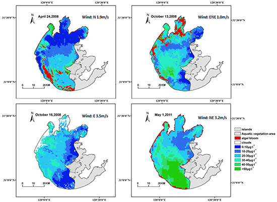
7.2. Application of the Spectral Decomposition Algorithm to Study Chla Spatial Distributions
7.3. The Spectral Decomposition Model Application to Other Satellite Data
8. Conclusions
Acknowledgments
Conflicts of Interest
- Author ContributionsYuchao Zhang had the original idea for the study and with all co-authors carried out the design. Ronghua Ma was responsible for recruitment and follow-up of study participants. Jinduo Xu was responsible for data cleaning. Hongtao Duan and Yuchao Zhang carried out the analyses. Yuchao Zhang drafted the manuscript, which was revised by Steven Loiselle. All authors read and approved the final manuscript.
References
- Ma, R.H.; Duan, H.T.; Tang, J.W.; Chen, Z.B. Remote Sensing of Lake Water Environment; Science Publication: Beijing, China, 2010. (In Chinese) [Google Scholar]
- Morel, A.; Prieur, L. Analysis of variations in ocean color. Limnol. Oceanogr 1977, 22, 709–722. [Google Scholar]
- Gordon, H.R.; Morel, A.Y. Remote Assessment of Ocean Color for Interpretation of Satellite Visible Imagery: A Review. In Lecture Notes on Coastal and Estuarine Studies; Springer-Verlag: Berlin, Germany, 1983; p. 114. [Google Scholar]
- Sathyendranath, S.; Morel, A. Light emerging from the sea-interpretation and uses in remote sensing. Remote Sens. Appl. Mar. Sci. Technol 1983, 106, 323–357. [Google Scholar]
- IOCCG, Remote Sensing of Ocean Colour in Coastal, and Other Optically-Complex Waters. In Reports of the International Ocean-Colour Coordinating Group; Sathyendranath, S. (Ed.) IOCCG: Dartmouth, NS, Canada, 2000; pp. 12–17.
- Dekker, A.G. Detection of Optical Water Quality Parameters for Eutrophic Waters by High Resolution Remote Sensing. In Doctorate Thesis in Earth and Life Sciences; Vrijie Universiteit: Amsterdam, The Netherlands, 1993; pp. 10–13. [Google Scholar]
- Gons, H.J. Optical teledetection of chlorophyll-a in turbid inland waters. Environ. Sci. Technol 1999, 33, 1127–1132. [Google Scholar]
- Gitelson, A.A.; Dall’Olmo, G.; Moses, W.M.; Rundquist, D.C.; Barrow, T.; Fisher, T.R.; Gurlin, D.; Holz, J. A simple semi-analytical model for remote estimation of chlorophyll-a in turbid waters: Validation. Remote Sens. Environ 2008, 112, 3582–3593. [Google Scholar]
- Dall’Olmo, G.; Gitelson, A.A. Effect of bio-optical parameter variability on the remote estimation of chlorophyll-a concentration in turbid productive waters: Experimental results. Appl. Opt 2005, 44, 412–422. [Google Scholar]
- Zimba, P.V.; Gitelson, A. Remote estimation of chlorophyll concentration in hyper-eutrophic aquatic systems: Model tuning and accuracy optimization. Aquaculture 2006, 256, 272–286. [Google Scholar]
- Le, C.F.; Li, Y.M.; Zha, Y.; Sun, D.Y.; Huang, C.C.; Lu, H. A four-band semi-analytical model for estimating chlorophyll-a in highly turbid lakes: The case of Taihu Lake, China. Remote Sens. Environ 2009, 113, 1175–1182. [Google Scholar]
- Duan, H.T.; Ma, R.H.; Zhang, Y.Z.; Loiselle, S.A.; Xu, J.P.; Zhao, C.L.; Zhou, L.; Shang, L.L. A new three-band algorithm for estimating chlorophyll concentrations in turbid inland lakes. Environ. Res. Lett 2010, 5, 1–6. [Google Scholar]
- Yang, W.; Bunki, M.; Chen, J.; Fukushima, T.; Ma, R.H. An enhanced three-band index for estimating Chlorophyll-a in turbid Case-II waters: Case studies of Lake Kasumigaura, Japan, and Lake Dianchi, China. IEEE Geosci. Remote Sens. Lett 2010, 7, 655–659. [Google Scholar]
- Li, Y.M.; Wang, Q.; Wu, C.Q.; Zhao, S.H.; Xu, X.; Wang, Y.F.; Huang, C.C. Estimation of chlorophyll-a concentration using NIR/Red bands of MERIS and classification procedure in inland turbid water. IEEE Trans. Geosci. Remote Sens 2012, 50, 988–997. [Google Scholar]
- Pilorz, S.H.; Davis, C.O. Spectral Decomposition of Sea Surface Reflected Radiance. Proceedings of the Geoscience and Remote Sensing Symposium, IGARSS ’90, ‘Remote Sensing Science for the Nineties’, 10th Annual International, University of Maryland, College Park, MD, USA, 20–24 May 1990; pp. 345–348.
- Novo, E.M.; Shimabukuro, Y.E. Spectral mixture analysis of inland tropical waters. Int. J. Remote Sens 1994, 15, 1351–1356. [Google Scholar]
- Tyler, A.N.; Svab, E.; Preston, T.; Présing, M.; Kovács, W.A. Remote sensing of the water quality of shallow lakes: A mixture modelling approach to quantifying phytoplankton in water characterized by high suspended sediment. Int. J. Remote Sens 2006, 27, 1521–1537. [Google Scholar]
- Sváb, E.; Tyler, A.N.; Preston, T.; Présing, M.; Balogh, K.V. Characterizing the spectral reflectance of algae in lake waters with high suspended sediment concentrations. Int. J. Remote Sens 2005, 26, 919–928. [Google Scholar]
- Novo, E.M.; Barbosa, C.C.; Freitas, R.M.; Shimabukuro, Y.E.; Melack, J.M.; Filho, W.P. Seasonal changes in chlorophyll distributions in Amazon floodplain lakes derived from MODIS images. Limnology 2006, 7, 153–161. [Google Scholar]
- Oyama, Y.; Matsushita, B.; Fukushima, T.; Naqai, T.; Imai, A. A new algorithm for estimating chlorophyll-a concentration from multi-spectral satellite data in case II waters: A simulation based on a controlled laboratory experiment. Int. J. Remote Sens 2007, 28, 1437–1453. [Google Scholar]
- Oyama, Y.; Matsushita, B.; Fukushima, T.; Matsushige, K.; Imai, A. Application of spectral decomposition algorithm for mapping water quality in a turbid lake (Lake Kasumigaura, Japan) from Landsat TM data. ISPRS J. Photogramm. Remote Sens 2009, 64, 73–85. [Google Scholar]
- Oyama, Y.; Matsushita, B.; Fukushima, T.; Chen, J.; Naqai, T.; Imai, A. Testing the spectral decomposition algorithm (SDA) for different phytoplankton species by a simulation based on tank experiments. Int. J. Remote Sens 2010, 31, 1605–1623. [Google Scholar]
- Xiao, C.; Wen, J.G.; Liu, Q.H.; Zhou, Y. Study on spectral unmixing model and its application in extracting chlorophyll concentration of water body. J. Remote Sens 2006, 10, 559–567. (In Chinese) [Google Scholar]
- Qian, S.; Lin, Q.Z.; Chen, X. An improved method of spectral unmixing of remote sensing image and its application in water pollution monitoring and assessing. Geogr. Geo-Inf. Sci 2003, 19, 36–38. (In Chinese) [Google Scholar]
- Zheng, Y.F.; Fan, W.H.; Zhang, X.F.; Wu, R.J. Pixel unmixing technology of MODIS remote sensing data. J. Nanjing Inst. Meteorol 2008, 31, 145–150. (In Chinese) [Google Scholar]
- Lu, C.P.; Lv, H.; Li, Y.M. Algorithms based on spectral decomposition algorithm for retrieval of constituents in Taihu Lake. J. Geo-Inf. Sci 2012, 13, 687–694. (In Chinese) [Google Scholar]
- Mertes, L.A.K.; Daniel, D.L.; Melack, J.M.; Nelson, B.; Martinelli, L.A.; Forsberg, B.R. Spatial patterns of hydrology, geomorphology, and vegetation on the floodplain of the Amazon River in Brazil from a remote sensing perspective. Geomorphology 1995, 13, 215–232. [Google Scholar]
- Mobley, C.D. Light and Water: Radiative Transfer in Natural Waters; Academic Press: New York, NY, USA, 1994. [Google Scholar]
- Ma, R.; Jiang, G.; Duan, H.; Bracchini, L.; Loiselle, S.A. Effective upwelling irradiance depths in turbid waters: A spectral analysis of origins and fate. Opt. Express 2011, 19, 7127–7138. [Google Scholar]
- Wang, C.F.; Duan, H.T.; Ma, R.H.; Zhang, Y.C. Inherent optical properties of large lakes in the middle-lower reaches of the Yangtze River: I Absorption. J. Lake Sci 2013, 25, 497–504. (In Chinese) [Google Scholar]
- Cai, Q.; Gao, X.; Chen, Y.; Ma, S.; Dokulil, M. Dynamic variations of water quality in Lake Taihu and multivariate analysis of its influential factors. Chin. Geogr. Sci 1996, 6, 364–374. [Google Scholar]
- Chen, Y.W.; Qin, B.Q.; Teubner, K.; Dokulil, M. Long-term dynamics of phytoplankton assemblages: Microcystis- domination in a large shallow lake in China. J. Plankton Res 2003, 25, 445–453. [Google Scholar]
- Duan, H.; Ma, R.; Zhang, Y.; Loiselle, S.A. Are algal blooms occurring later in Lake Taihu? Climate local effects outcompete mitigation prevention. J. Plankton Res 2014, 2014. [Google Scholar] [CrossRef]
- Guo, L. Doing battle with the green monster of Taihu Lake. Science 2007, 317. [Google Scholar] [CrossRef]
- Duan, H.T.; Ma, R.H.; Xu, X.F.; Kong, F.X.; Zhang, S.X.; Kong, W.J.; Hao, J.Y.; Shang, L.L. Two-decade reconstruction of algal blooms in China’s Lake Taihu. Environ. Sci. Technol 2009, 43, 3522–3528. [Google Scholar]
- Cai, Y.F. Comparative Study of Composition and Dynamics of Cyanobacteria and Their Driving Factors in Lake Taihu and Lake Chaohu. Ph.D Thesis, Nanjing Institute of Geography and Limnology, Chinese Academy of Sciences, Nanjing, China, 30 May 2009. [Google Scholar]
- Hu, C.H.; Hu, W.P.; Zhang, F.B.; Hu, Z.X.; Li, X.H.; Chen, Y.G. Sediment resuspension in the Lake Taihu, China. Chin. Sci. Bull 2006, 51, 731–737. [Google Scholar]
- Zhang, Y.L.; Qin, B.Q.; Ma, R.H.; Zhu, G.W.; Zhang, L.; Chen, M.W. Chromophoric dissolved organic matter absorption characteristics with relation to fluorescence in typical macrophyte, algae lake zones of Lake Taihu. Environ. Sci 2005, 26, 142–147. (In Chinese) [Google Scholar]
- Pope, R.M.; Fry, E.S. Absorption spectrum (380–700 nm) of pure water. II. Integrating cavity measurements. Appl. Opt 1997, 36, 8710–8723. [Google Scholar]
- Mueller, J.L.; Fargion, G.S.; McClain, C.R. Ocean Optics Protocols for Satellite Ocean Color Sensor. In Special Topics in Ocean Optics Protocols and Appendices; Goddard Space Flight Center: Greenbelt, MD, USA, 2003; pp. 52–63. [Google Scholar]
- Rast, M.; Bezy, J.L.; Bruzzi, S. The ESA medium resolution imaging spectrometer MERIS a review of the instrument and its mission. Int. J. Remote Sens 1999, 20, 1681–1702. [Google Scholar]
- Gons, H.J.; Auer, M.T.; Effler, S.W. MERIS satellite chlorophyll mapping of oligotrophic and eutrophic waters in the Laurentian Great Lakes. Remote Sens. Environ 2008, 112, 4098–4106. [Google Scholar]
- Alikas, K.; Reinart, A. Validation of the MERIS products on large European lakes: Peipsi, Vänern and Vättern. Hydrobiologia 2008, 599, 161–168. [Google Scholar]
- Duan, H.T.; Ma, R.H.; Simis, S.G.H.; Zhang, Y.Z. Validation of MERIS case-2 water products in Lake Taihu, China. GIS Sci. Remote Sens 2012, 49, 873–894. [Google Scholar]
- Earth Observation Toolbox and Development Platform. Available online: http://www.brockmann-consult.de/cms/web/beam (accessed on 26 May 2013).
- Gitelson, A.; Garbuzov, G.; Szilagyi, F.; Mittenzwey, K-H.; Karnieli, A. Quantitative remote sensing methods for real-time monitoring of inland waters quality. Int. J. Remote Sens 1993, 14, 1269–1295. [Google Scholar]
- Schalles, J.F.; Gitelson, A.; Yacobi, Y.Z.; Kroenke, A.E. Estimation of chlorophyll from time series measurements of high spectral resolution reflectance in a eutrophic lake. J. Phycol 1998, 34, 383–390. [Google Scholar]
- Gordon, H. Diffusive reflectance of the ocean: The theory of its augmentation by chlorophyll-a fluorescence at 685 nm. Appl. Opt 1979, 18, 1161–1166. [Google Scholar]
- Moses, W.J.; Gitelson, A.A.; Berdnikov, S.; Povazhnyy, V. Satellite estimation of chlorophyll-a concentration using the red and NIR bands of MERIS—The Azov Sea case study. IEEE Geosci. Remote Sens. Lett 2009, 6, 845–849. [Google Scholar]
- Mishra, S.; Mishra, D.R. Normalized difference chlorophyll index: A novel model for remote estimation of chlorophyll-a concentration in turbid productive waters. Remote Sens. Environ 2012, 117, 394–406. [Google Scholar]
- Zhou, L. Remote Sensing Retrieval of Chlorophyll-a Concentration in Lake Waters. Master’s Thesis, Nanjing Institute of Geography and Limnology, Chinese Academy of Sciences, Nanjing, China, 30 May 2011. [Google Scholar]
- Sosik, H.M.; Mitchell, B.G. Light absorption by phytoplankton, photosynthetic pigments and detritus in the California current system. Deep-Sea Res 1995, 42, 1717–1748. [Google Scholar]
- Stramska, M.; Frye, D. Dependence of apparent optical properties on solar altitude: Experimental results based on mooring data collected in the Sargasso Sea. J. Geogr. Res 1997, 102, 15679–15691. [Google Scholar]
- Kirk, J.T.O. Dependence of relationship between inherent and apparent optical properties of water on solar altitude. Limnol. Oceanogr 1984, 29, 350–356. [Google Scholar]
- Zhang, M.; Kong, F.; Wu, X.; Xing, P. Different photochemical responses of phytoplankters from the large shallow Taihu Lake of subtropical China in relation to light and mixing. Hydrobiologia 2008, 603, 267–278. [Google Scholar]
- Kong, F.X.; Song, L.R. Cynobacteria Blooms Formation and Its Environmental Factors; Science Press: Beijing, China, 2011. (In Chinese) [Google Scholar]
- Cao, H.S.; Kong, F.X.; Luo, L.C.; Shi, X.L.; Yang, Z.; Zhang, X.F.; Tao, Y. Effects of wind and wind-induced waves on vertical phytoplankton distribution and surface blooms of microcystis aeruginosa in Lake Taihu. J. Freshw. Ecol 2006, 21, 231–238. [Google Scholar]
- Huang, Y.P. Water Environment and Its Pollution Control in Lake Taihu; Science Press: Beijing, China, 2010. (In Chinese) [Google Scholar]
- Odermatt, D.; Vittorio Ernesto Brando, A.G.; Schaepman, M. Review of constituent retrieval in optically deep and complex waters from satellite imagery. Remote Sens. Environ 2012, 118, 116–126. [Google Scholar] [Green Version]
- Matthews, M.W.; Bernard, S.; Robertson, L. An algorithm for detecting trophic status (chlorophyll-a), cyanobacterial-dominance, surface scums and floating vegetation in inland and coastal waters. Remote Sens. Environ 2012, 124, 637–652. [Google Scholar]


| Data Type | Numbers | Minimum | Maximum | Mean | SD | CV |
|---|---|---|---|---|---|---|
| 27 March 2011 | 33 | 5.45 | 31.05 | 16.82 | 6.53 | 0.39 |
| 3 September 2011 | 27 | 13.13 | 160.93 | 49.78 | 38.90 | 0.78 |
| 24 April 2008 | 11 | 7.76 | 58.5 | 26.53 | 18.90 | 0.71 |
| 13 October 2008 | 8 | 4.16 | 14.81 | 9.86 | 3.63 | 0.37 |
| 16 October 2008 | 21 | 10.86 | 43.56 | 20.86 | 7.92 | 0.38 |
| 1 May 2011 | 12 | 5.28 | 37.06 | 18.36 | 10.24 | 0.56 |
| Models | MERIS Bands | Function with Cp | R2 | RE (%) | RMSE (μg·L−1) |
|---|---|---|---|---|---|
| M1 | 2,5,7,9 | y = 8.7261Cp2 − 3.4274Cp + 15.119 | 0.6147 | 46.50 | 30.40 |
| M2 | 2,5,7,10 | y = 0.1353Cp2 − 13.153Cp + 19.107 | 0.5750 | 51.29 | 32.04 |
| M3 | 2,5,8,9 | y = 0.0204Cp2 + 0.884Cp + 26.684 | 0.5246 | 62.91 | 33.89 |
| M4 | 2,5,8,10 | y = 0.44Cp2 − 10.25Cp + 41.46 | 0.4813 | 137.15 | 35.39 |
| M5 | 3,5,7,9 | y = 19.214e0.856Cp | 0.7722 | 33.58 | 20.62 |
| M6 | 3,5,7,10 | y = 1.8896Cp2 − 18.66Cp + 56.518 | 0.7449 | 54.54 | 24.82 |
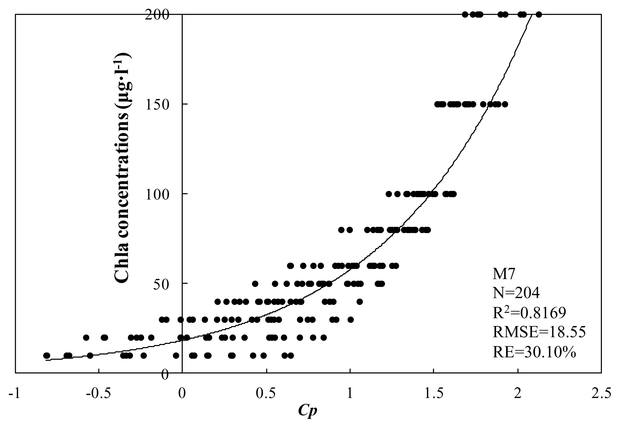
| M7 | 3,5,8,9 | y = 18.219e1.1498Cp | 0.8169 | 30.10 | 18.55 |
| M8 | 3,5,8,10 | y = 42.903e1.2412Cp | 0.5552 | 52.78 | 33.00 |
| Range | Samples | RMSE (μg·L−1) | RE (%) |
|---|---|---|---|
| 0 < Chla ≤ 10 μg·L−1 | 4 | 6.04 | 86.89 |
| 10 < Chla ≤ 20 μg·L−1 | 27 | 5.82 | 31.85 |
| 20 < Chla ≤ 30 μg·L−1 | 10 | 8.22 | 28.22 |
| 30 < Chla ≤ 40 μg·L−1 | 7 | 9.58 | 23.46 |
| 40 < Chla ≤ 50 μg·L−1 | 2 | 20.76 | 47.98 |
| 50 μg·L−1 < Chla | 10 | 7.98 | 7.57 |
| Model | Bands Combination | RMSE (μg L−1) | RE (%) |
|---|---|---|---|
| LI-1 model | 12.76 | 55.71 | |
| LI-2 model | 16.41 | 61.62 | |
| LI-3 model | 10.56 | 51.62 | |
| LI-4 model | 10.01 | 53.82 | |
| LI-5/Moses’ model | Rrs(b9)/Rrs(b7) | 13.59 | 60.56 |
| LI-6 model | Rrs(b9)/Rrs(b8) | 14.78 | 53.00 |
| Zhou’s model | 8.75 | 64.56 | |
| Mishra’s model | (Rrs(b9) − Rrs(b7))/(Rrs(b9) + Rrs(b7)) | 10.98 | 54.64 |
| New model | M7(band 3,5,8,9) | 8.45 | 58.06 |
| Range | Time | |||
|---|---|---|---|---|
| 24 April 2008 | 13 October 2008 | 16 October 2008 | 1 May 2011 | |
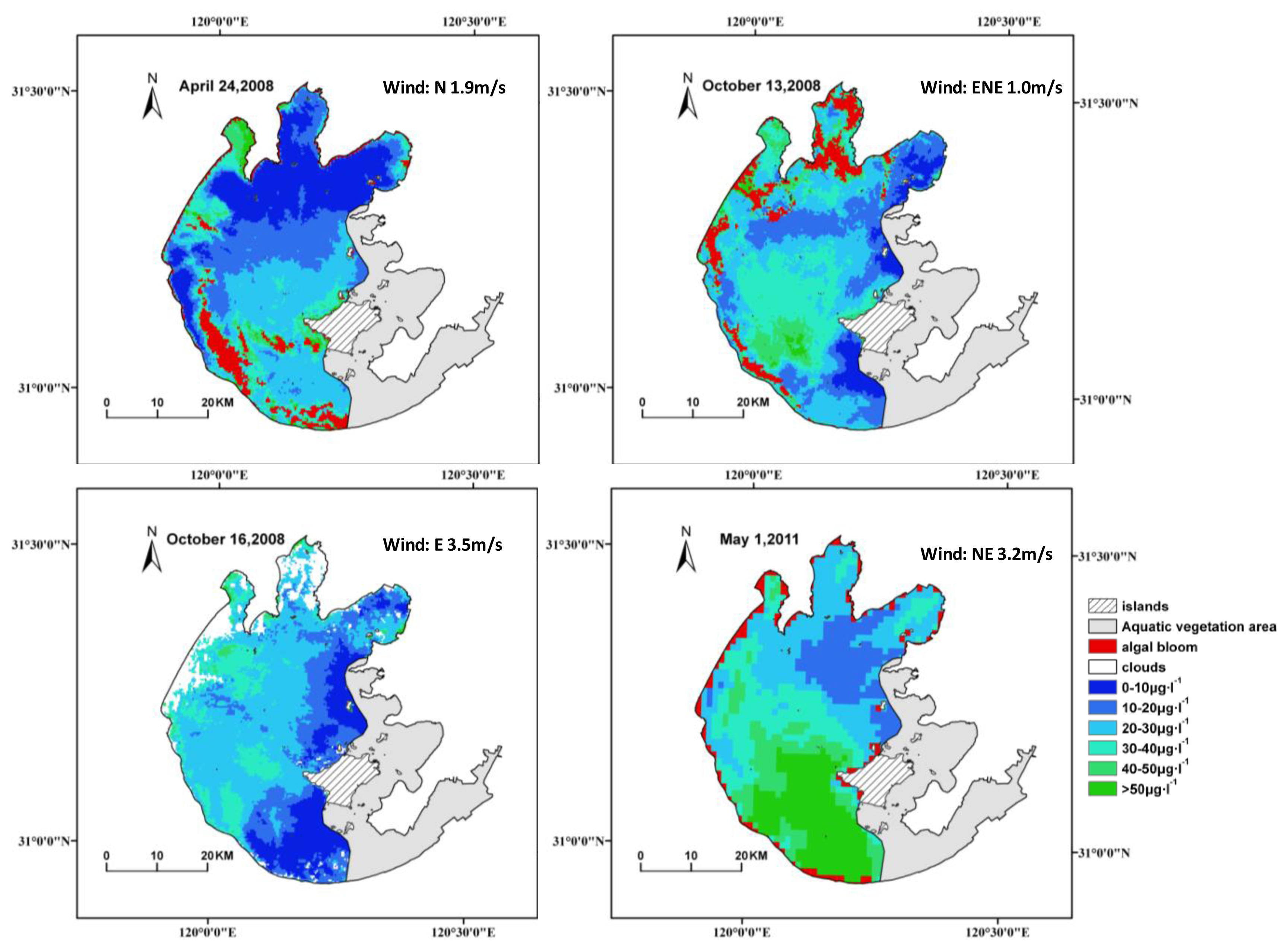
| 0 < Chla ≤ 10 μg·L−1 | 22.27% | 9.24% | 17.78% | 0% |
| 10 < Chla ≤ 20 μg·L−1 | 26.03% | 21.92% | 21.13% | 16.12% |
| 20 < Chla ≤ 30 μg·L−1 | 30.84% | 32.76% | 41.13% | 33.52% |
| 30 < Chla ≤ 40 μg·L−1 | 10.67% | 21.47% | 14.01% | 22.86% |
| 40 < Chla ≤ 50 μg·L−1 | 7.28% | 11.24% | 3.18% | 12.07% |
| The rest | 2.91% | 3.38% | 2.77% | 15.44% |
© 2014 by the authors; licensee MDPI, Basel, Switzerland This article is an open access article distributed under the terms and conditions of the Creative Commons Attribution license (http://creativecommons.org/licenses/by/3.0/).
Share and Cite
Zhang, Y.; Ma, R.; Duan, H.; Loiselle, S.; Xu, J. A Spectral Decomposition Algorithm for Estimating Chlorophyll-a Concentrations in Lake Taihu, China. Remote Sens. 2014, 6, 5090-5106. https://doi.org/10.3390/rs6065090
Zhang Y, Ma R, Duan H, Loiselle S, Xu J. A Spectral Decomposition Algorithm for Estimating Chlorophyll-a Concentrations in Lake Taihu, China. Remote Sensing. 2014; 6(6):5090-5106. https://doi.org/10.3390/rs6065090
Chicago/Turabian StyleZhang, Yuchao, Ronghua Ma, Hongtao Duan, Steven Loiselle, and Jinduo Xu. 2014. "A Spectral Decomposition Algorithm for Estimating Chlorophyll-a Concentrations in Lake Taihu, China" Remote Sensing 6, no. 6: 5090-5106. https://doi.org/10.3390/rs6065090