
Improvement Method of Antenna Negative Sidelobes on Cross Beam Correlation Microwave Radiometer

1
The Key Laboratory of Microwave Remote Sensing, National Space Science Center, Chinese Academy of Sciences, Beijing 100190, China
2
The School of Electronic, Electrical and Communication Engineering, University of Chinese Academy of Sciences, Beijing 100049, China
*
Author to whom correspondence should be addressed.
Remote Sens. 2024, 16(7), 1245; https://doi.org/10.3390/rs16071245
Submission received: 29 January 2024
/
Revised: 29 March 2024
/
Accepted: 30 March 2024
/
Published: 31 March 2024
(This article belongs to the Section Engineering Remote Sensing)
Abstract
:A weighting method is proposed for the correlation radiation measurement system based on Mills cross array. The Mills cross array achieves high spatial resolution by the product of two orthogonal fan beams. However, the product power pattern of the Mills cross array lacks a square operation, resulting in sidelobe deterioration and the presence of negative sidelobes. Therefore, a window function is necessary to improve beam performance. However, because of the negative sidelobes, the antenna array is sensitive to the weighting function, and common window functions such as Hanning and Hamming are not suitable for achieving optimal antenna performance. A weighting method is proposed to fully utilize the feature that the received energy of positive and negative sidelobes cancel each other out and to reduce the influence of antenna sidelobe errors in radiation measurement. Such a weighting function can be obtained by combining the combined cosine window function with the existing particle swarm optimization (PSO). The optimized window function is evaluated through numerical simulation and compared with the typical window function weighting results. The results show that this weighting method can minimize the impact of negative sidelobes and reduce the loss of spatial resolution.
1. Introduction
The Mills cross measurement system processes the received signals of two orthogonal fan beams and achieves “pencil” beam observation at the intersection of the fan beams [1,2]. This system was first used in astronomy [3,4,5] and is a simple, small-area, low-cost antenna system design solution. In recent years, advancements in digital signal processing technology and microwave technology have led to their gradual application in the field of microwave remote sensing [6,7,8,9]. Compared to a filled array antenna, this design ensures resolution while significantly reducing the number of antenna elements and simplifying antenna design. In contrast, compared to synthetic aperture radiometers using sparse arrays, the measurement system significantly reduces the cost and system complexity, making it sufficiently attractive for remote sensing observations.
The basic structure of the Mills cross array is a “cross”, which consists of two long antennas arranged orthogonally in space, as illustrated in Figure 1. The array elements are evenly distributed on the two antenna arms to form two orthogonal fan-shaped beams. The coherence of the signals in the overlapping region of the beams is utilized to achieve the observation effect of a “pencil” beam.
For the measurement model depicted in Figure 1, the correlation result of the output signals of the two sector beams can be expressed as [10,11]:
where k is the Boltzmann constant, is the brightness temperature distribution of the scene, B is the receive bandwidth, are the normalized patterns of two subarrays with gains and , the components and are direction cosines ( and are the traditional spherical coordinates). From (1), the normalized power pattern of the Mills cross array, which is equivalent to the power pattern of the conventional antenna array, can be obtained
It can be found that the power pattern of the equivalent pencil beam of the Mills cross antenna array is directly obtained by multiplying the voltage patterns of the two subarrays, which is one less squaring operation than that of the power pattern of the conventional antenna array. As a result, the sidelobe of the equivalent product power pattern obtained from (2) deteriorates, which can have a large impact on the radiometric measurements [7,8], and a window function needs to be added to suppress the sidelobe level to improve the beam performance. Additionally, due to significant differences in the voltage patterns of the two sub-arrays, the phases of the two voltage patterns cannot be cancelled out through conjugate multiplication. As a result, the product power pattern of Mills cross antenna arrays will exhibit negative sidelobes [12], similar to the synthetic array factor of the synthetic aperture radiometer [13,14].
It is also important to note that the “negative” energy received by the negative sidelobe can cancel out some of the energy received by the positive sidelobe, or even make the overall energy received by the sidelobe negative, which can have an effect on the radiometric measurements. When the energy received by the positive and negative sidelobes is equal in magnitude, the sidelobe will not affect the observation of the main lobe, which is expected. Therefore, we aim for the weighted product power pattern to satisfy two main criteria: (1) low sidelobe level, and (2) equal positive and negative sidelobe solid angles, or at least a positive sidelobe solid angle greater than the negative sidelobe solid angle. Conventional weighting schemes can be used for sidelobe suppression of Mills cross array, but they are not optimal because they do not take into account the effect of the negative sidelobe of the array. In other words, they do not achieve the optimal performance of the antenna array under identical conditions.
In this paper, we propose a weighting method based on a combination of the cosine window function and the particle swarm optimization (CosW-PSO), which aims to fully utilize the negative sidelobe characteristic of the antenna power pattern in order to minimize the impact of antenna sidelobe errors.
2. Theoretical Analysis
Without considering the effect of antenna gain loss and antenna efficiency, the lossless antenna temperature of the Mills cross array can be expressed in terms of the main lobe mean brightness temperature and the sidelobe mean brightness temperature [15]:
where is the lossless antenna temperature and “” denotes the observation space . When analyzing the negative energy effects received by the negative sidelobe of the Mills cross array in detail, (3) is inappropriate because it treats all sidelobes as a single term. For this reason, the sidelobes are divided into two categories, positive and negative sidelobes, according to phase, and (3) is modified to be:
where and denote the sets of positive and negative sidelobes, respectively, and are main beam solid angle, positive sidelobe solid angle, and negative sidelobe solid angle, respectively, which can be expressed by the normalized product power pattern as
, and note that is negative. The pattern solid angle of is expressed by , which satisfies . can be obtained directly by radiometer measurement, and the estimate can be analytically obtained by (4).
The second term of Equation (6) is the measurement error term generated by the sidelobe.
The restriction of can be achieved by adding window functions. When there is a high demand for , a window function with strong suppression of the sidelobe level (SLL) is required. However, the more the SLL is suppressed by the window function, the greater the loss of the 3 dB beamwidth, which leads to a deterioration in spatial resolution. For antenna arrays with negative sidelobes, the energy received by the positive and negative sidelobes can cancel each other, and for this reason, we consider exploiting this property to reduce the beamwidth degradation by lowering the limit on SLL while ensuring the requirement of . Doing a deformation of (7),
In Equation (8), the measurement error caused by sidelobes is divided into two terms. The first term on the left represents the measurement error due to the difference in solid angle values between positive and negative sidelobes, and since is negative, this term is zero when . The second item on the left represents the measurement error caused by the difference in the average brightness temperature of the positive and negative sidelobe observation scenes, with a slope that is affected by the sidelobe level. Thus, we will find an interesting phenomenon that for antenna arrays with negative sidelobes, when the two conditions and are fulfilled, even though . Among all the influence factors of , , and are variables related to the observation scene that are not controlled. However, and are determined by the sidelobes of the antenna array, which can be adjusted by the window function. Therefore, the restriction on SLL can be reduced by designing the window function so that the antenna array satisfies the condition , which makes the first term error zero.
In the next section, we will discuss the feasibility of optimizing Equation (8) from two perspectives: the sidelobe distribution characteristics of the Mills cross array and the implementation of the array window function.
3. Negative Sidelobes and Window Function Design
3.1. Sidelobes Distribution Characteristics of Mills Cross Array
In order to achieve the positive and negative sidelobe solid angle equality by window function, the distribution characteristics of negative sidelobes in Mills cross array need to be known first [11].
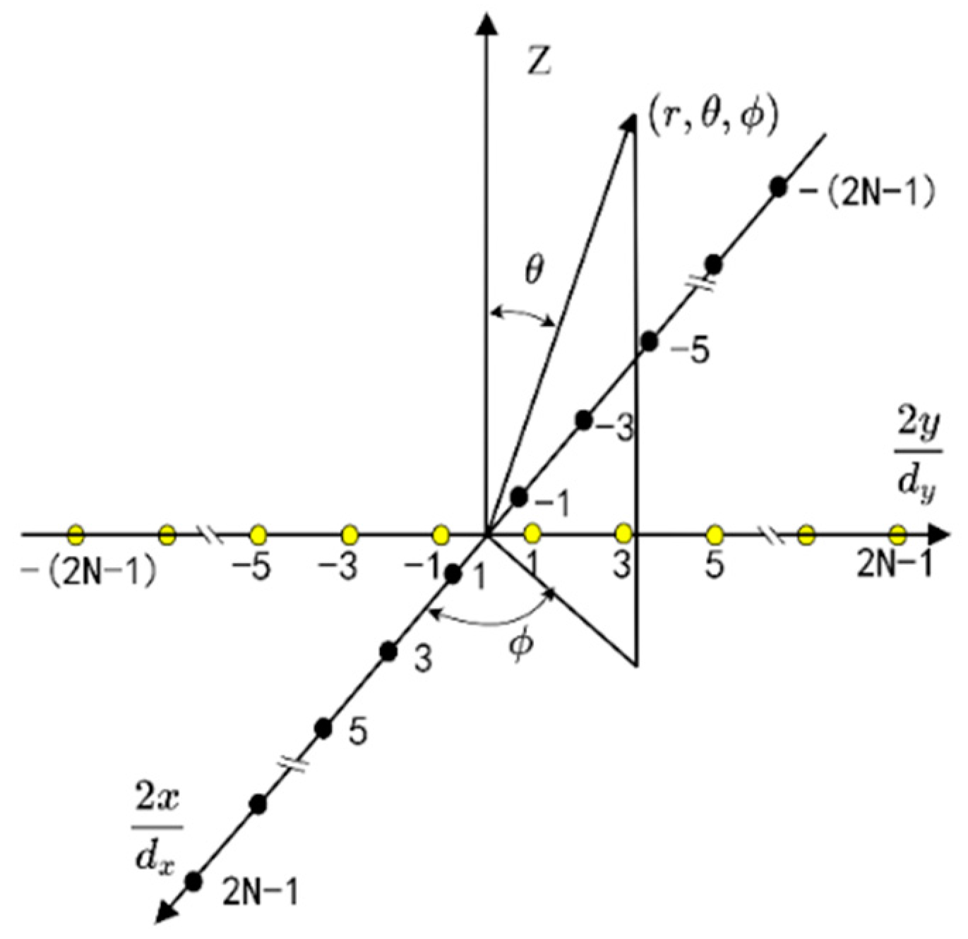
As shown in Figure 2, the two subarrays of the Mills cross array are zero-baseline but completely independent. Each subarray has an even number of antenna elements which are uniformly distributed on the antenna arms. When each array element is considered to isotropic source, the array factor of the Mills cross array is:
where 2N is the number of antenna units on each arm, is the antenna unit spacing on the corresponding arm, and .
Equation (9) corresponds to the power, but the subarray patterns of the two multiplying beams have large differences, so the conjugate multiplication does not zero out the phase of the product result. The product array factor of a Mills cross array can be approximated as the product of two sinc(·) functions. It is clear that for each sinc(·) function, starting from the main lobe, the phase of the sidelobes alternate between 0° and 180° in a striped pattern. According to (9), the phase distribution of the product array factor is obtained from phase difference in the voltage patterns of the two subarrays, with two phase values of 0° and 180° (−180°), which are alternately distributed in a grid pattern around the main lobe as the center, as shown in Figure 3.
It is obvious that since the positive and negative sidelobe of the Mills cross array are alternately distributed centered on the main lobe, it is feasible to make the first term in (8) zero by adding a window function. At the same time, the alternating distribution of positive and negative sidelobe also greatly reduces the difference between the observed scene average brightness temperature and , offering the possibility of relaxing the requirement of slope .
When the radiation patterns of individual array elements are identical, the product power pattern of a Mills cross array can be expressed as the product of the product array factor and the antenna element power pattern. Considering the array windowing at the same time, (9) becomes,
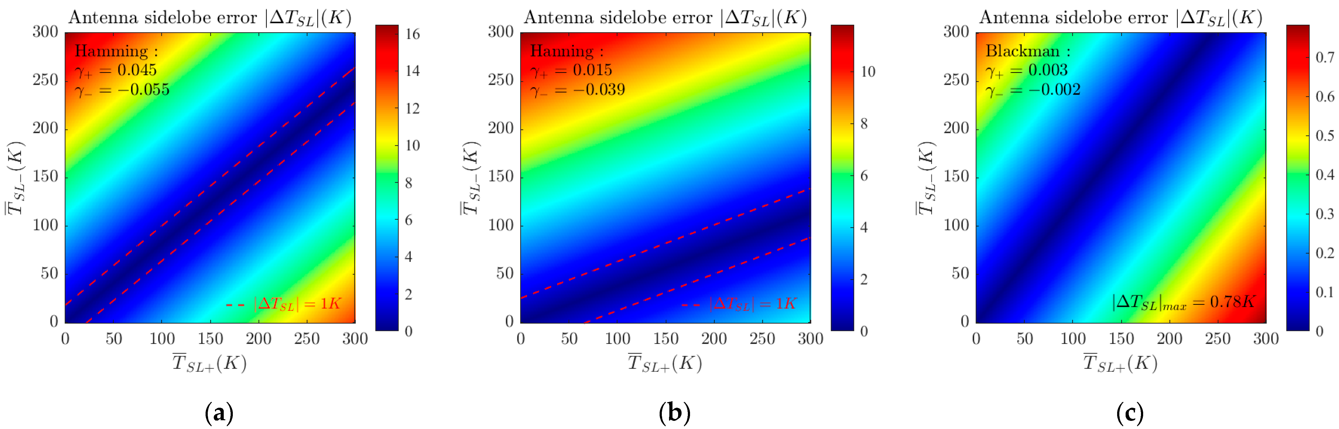
where is the array weighting coefficient and is the element antenna voltage pattern. However, the commonly used weighting functions are not fully applicable to achieve the antenna beam characteristic requirements described above. This is because the commonly used windowing functions are more concerned with the degree of suppression and the rate of decline of the sidelobe level without considering the energy ratio between the positive and negative sidelobes. Figure 4 shows the variation image of antenna sidelobe error with and after weighted by several common window functions, where .
As expected, when weighted by several common window functions, the absolute values of positive and negative sidelobe solid angles and are not equal. This causes the optimal solution of the sidelobe error in Figure 4 to deviate from the centerline . As can be seen from the beam characteristics of the Mills cross array, the values of and are similar. Therefore, we prefer that the optimal solution of occurs at .
In Figure 4c, the sidelobe error is less than 1 after Blackman weighting, but this is only the result of strong suppression of SLL, which results in a significant loss of spatial resolution. However, the above analysis shows that the first term on the right-hand side of (8) can be made zero by choosing an appropriate window function. At this time, there is no need for stronger suppression of the SLL to achieve the same or even smaller sidelobe error as when the Blackman window is added. And better spatial resolution than Blackman weighting can be obtained. This window function can be derived using particle swarm optimization.
3.2. Particle Swarm Optimization Algorithm
Particle swarm optimization (PSO) is a nonlinear optimization algorithm [16,17], which has been successfully applied to antenna array design problems [18,19,20,21]. In the PSO algorithm, each particle represents a candidate solution to the optimization problem and adjusts its position in the search space according to its own experience and the experience of the particle population. At each iteration, the particle swarms are evaluated by their fitness function to find the optimal solution for themselves and the population, and the process is repeated until the population is found to converge to the global optimum. The two basic equations for particle swarm position iteration are as follows:
where is the particle velocity matrix, is the current particle solution matrix, and are the best position of the individual particle and the best position of the group that has been found, respectively, is the inertia weight, and are acceleration constants, and the uniformly generated random numbers in the range of [0, 1] used to simulate the unpredictability of the group behavior.
Compared to other optimization algorithms, such as genetic algorithm (GA) and simulated annealing (SA), PSO is easier to understand and implement and does not require much preprocessing. Only a minimal amount of fitness evaluation is needed to construct the product power pattern of the Mills cross array with equal positive and negative sidelobes solid angles. And the detailed optimal configuration scheme is presented in the following subsection.
3.3. Window Function Optimization Based on Particle Swarm Algorithm
As described in Section 2, the optimization of in (8) lies in the two factors: the sum of the positive and negative sidelobe solid angles and the ratio of the negative sidelobe solid angle to the main lobe solid angle of the array pattern, which is a bi-objective optimization problem with two fitness functions that can be modeled as:
where is the optimization objective for the slope of the second error term in Equation (8), determined by the maximum possible positive and negative sidelobe average brightness temperature difference in the observation scene and the maximum antenna sidelobe error, , that the measurement system can tolerate. and are defined by (5). In fact, when , the error introduced by it is then less than , so the fitness function can be further modified as:
The use of the fitness Function (14) can speed up the optimization convergence by reducing the requirement of while satisfying the bias requirement. Next for the bi-objective optimization problem described in (13) and (14), we simply use the conventional weighted aggregation (CWA) method to deal with it, forming a single-objective optimization by weighting the factors
In the equation, the weight coefficients and are two real numbers between [0, 1], which satisfy . In this case, and are used. In addition, it is worth discussing that the CWA method is used here instead of vector-evaluated PSO (VEPSO) [22] or MOPSO (d-MOPSO) [23], because the level of importance for the two factors in (13) is clear. Therefore, the determination of the weighting coefficients , is simpler, and the optimal solution meeting the requirements can be obtained [15]. The d-MOPSO method greatly increases the complexity of the algorithm because it introduces the concept of Pareto dominance [24].
For the Mills cross array depicted in Figure 2, the optimization of (15) is achieved by iterating over the weighted window functions of the two subarrays. Considering that the two subarrays have the same antenna configuration, the same window function () can be used, reducing the dimension of the search space of the particle swarm optimizer to half of the original size. The specific implementation of particle swarm optimization has two routes:
- (1)
- Particle swarm optimization weight function value: The PSO algorithm directly implements iterations on the weighting values [25], and the search space has a dimension of 2N, which is the length of the window function on each arm. This approach has a wider solution space but does not guarantee the sidelobe characteristics of the optimized pattern, such as sidelobe distribution spacing and sidelobe level decline characteristics, which may cause large tail lobes.
- (2)
- Particle swarm optimization of the combined term coefficients of the combined cosine window: The PSO algorithm iteratively combines term coefficients of the combined cosine window, and then calculates the weighting function value of the array using the updated combined term coefficients. The dimension of the search space is reduced from 2N to P + 1 (where P is the number of the terms in the function of the combined cosine window, generally 2 or 3). This optimization scheme can effectively leverage prior knowledge of the combined cosine window to expedite the optimization process. At the same time, the optimized window function can inherit the favorable performance of the combined cosine window, so the optimized pattern tends to exhibit good sidelobe performance.
The initial population particles of the standard PSO algorithm are randomly assigned, ignoring the available prior knowledge and resulting in the optimization converging too slowly or falling into a local optimum. To address this, we aim to optimize the initial value and the space range of constraint solutions by utilizing existing experience of window functions, so as to obtain the optimal solution that meets the requirements. The combined cosine window functions are flexible and diverse and can generate excellent cosine window functions [26], such as the Hanning window, Hamming window, Blackman window, and so on. Therefore, we use the combined cosine window function in the PSO algorithm to speed up the optimization solution. For a linear subarray with 2N antenna elements, the general expression for the combined cosine window function can be expressed as:
where P is the number of terms of the combined cosine window function; is a real constant coefficient not less than 0; = , , denotes the distance between the nth antenna element and the center of the array; and , which is generally taken to be equal, i.e., the distance between the furthest antenna unit and the center of the array.
It can be found that the array weighting coefficient is jointly constrained by the number of cosine terms , coefficients and . The combined term coefficient optimization is to optimize , and by particle swarm optimization algorithm, and then obtain the optimal solution of the weighted coefficient by (16). It should be noted that before PSO optimization, we need to determine the number of cosine terms , and afterward the iteration coefficient dimension
At each iteration, are the results after dividing their sum to satisfy . After bringing (17) into (16), if a particle have , to ensure that the array weighting factor is greater than 0, the following substitution is made
where are the classical coefficients of the P-order combinatorial cosine window and are the weighting coefficients obtained by bringing the classical coefficients into (16).
The particle swarm optimization flowchart using the proposed optimal combination of cosine window coefficients strategy is shown in Figure 5. The optimization scheme of the particle swarm algorithm using this strategy can be described as:
- Step 1: Determine the value of the combined cosine term P and initialize the particle swarm using the existing P-order cosine window function according to the desired value;
- Step 2: For each particle use (16) to calculate the weighting function value of the array (when , let ), bring in (10) to obtain the product power pattern of Mills cross array;
- Step 3: Evaluate the fitness of each particle, using fitness Function (15);
- Step 4: Compare the fitness of each particle to its best fitness. If , then , ;
- Step 5: Compare the fitness of each particle with the global optimal particle. If , then , ;
- Step 6: Update the velocity and position of all the particles;
- Step 7: Repeat steps 2 to 6 until satisfies the design requirements, output the global optimal solution , then compute the optimized solution of the weighted window function from (16).
4. Numerical Simulation
In order to verify the performance of the above PSO and combined cosine window function (CosW-PSO) algorithm and evaluate the improvement of the optimized antenna pattern with respect to the sidelobe error, two experiments are conducted in this section. The first is to compare the antenna pattern optimization capabilities of the CosW-PSO scheme proposed in Section 3.3 with the traditional PSO scheme using cosine window initial value optimization (Con-PSO). The second is to test the optimized pattern performance using common natural scenarios and compare it with the observed performance of the traditional weighted pattern.
4.1. Pattern Optimization Using CosW-PSO
For Mills cross array with given array elements of 3030, the PSO strategy shown in Figure 5 was used to optimize the antenna pattern. The subarray element spacing was set to , and the element pattern was replaced by a normalized Gaussian function with a value of −15 dB at .
In the numerical simulation, the basic parameters of the PSO algorithm are set as and P = 3, which are used to perform the PSO optimization of two values: (1) ; (2) , increasing the requirement of antenna sidelobe error . Each optimization was performed for 300 iterations using 30 populations. The convergence curves of the fitness Function (15) for two values of are given in Figure 6 and compared with the convergence curves using the conventional PSO scheme. It is clearly shown that although both schemes can reach the global optimum, CosW-PSO converges at 80 iterations, while Con-PSO requires at least 250 iterations to reach convergence. That is to say, the CosW-PSO scheme greatly improves the convergence characteristics, especially the convergence speed.
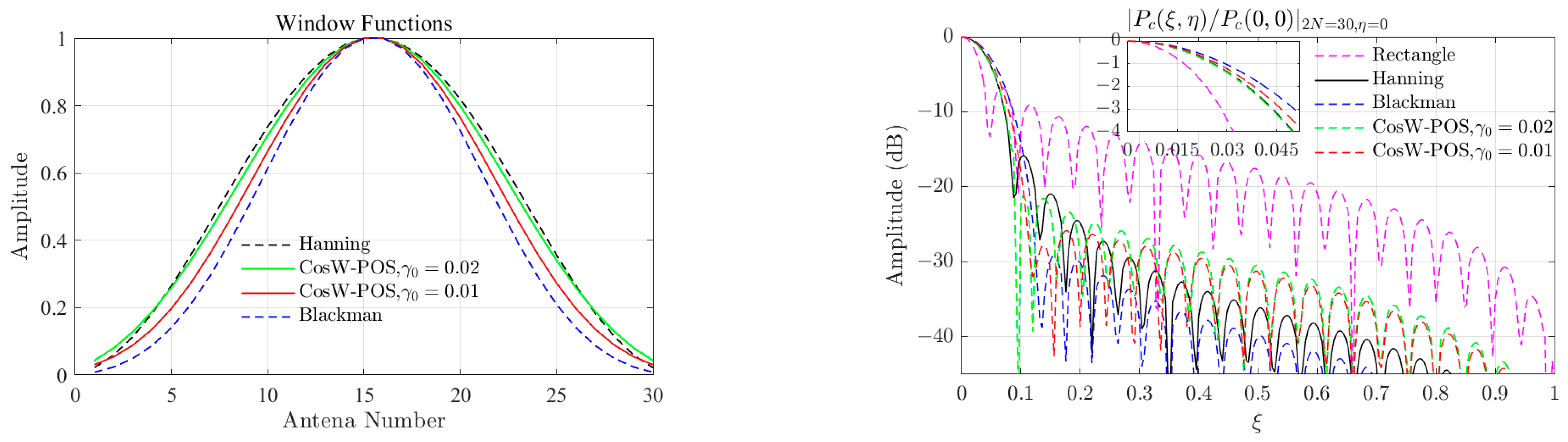
The combined cosine window coefficients obtained from the CosW-PSO optimization are shown in Table 1, and the corresponding optimization window function and Con-PSO optimization window function are compared in Figure 7. Although both optimization schemes result in globally optimal solutions, it is clear that their weighting factors are completely different. In contrast, the window function curves obtained by CosW-PSO are much smoother, and the performance of the multiplicative beams obtained by them will be dramatically different, as shown in Figure 8.
Figure 8 shows the optimized patterns of CosW-PSO and Con-PSO schemes when . It can be obviously found that the sidelobes of the product power pattern obtained from the CosW-PSO optimization are equally spaced in the space, and thus are reflected in the observation space as densely and uniformly distributed sidelobes, which is the desired characteristic of the pattern optimization. Because of the alternating distribution of positive and negative sidelobe s, the denser and more homogeneous their distribution in the observation space, the smaller will be the difference between the average positive and negative sidelobe brightness temperatures during measurement. According to (8), when the first term on the right is zero and the requirement of sidelobe error is unchanged, the average brightness temperature difference () in positive and negative sidelobes becomes smaller, and the requirement on the slope decreases, which allows relaxing the suppression of the SLL by the array weighting and decreasing the loss of spatial resolution due to the weighting. Meanwhile, it can be found that the sidelobe optimized by CosW-PSO decreases with the increase in , and has a good decay rate, which can effectively reduce the influence of the temperature source in the region of a large observation angle. The optimized antenna directional map obtained by using the Con-PSO scheme has an uneven distribution of positive and negative sidelobes, and larger sidelobes appear at large observation angles, which is not the desired result of the optimization.
In contrast, the optimization results of CosW-PSO are fully consistent with the optimal solution of the expected product power pattern. This is because the array weighting values obtained by the CosW-PSO strategy are computed by (16), which is a combined cosine window function under the optimization of a specific objective, and thus can inherit the properties of the combined cosine window function in terms of the suppression of the sidelobes and sidelobe decay speed, as well as specification of the location of the zero point of the patterns. The Con-PSO strategy, on the other hand, does not have the ability to constrain this feature during the optimization process because it is directly searching in a larger weighting function solution space, which is large but does not add the optimization objectives of the sidelobe decay rate and the zero position during the optimization. Thus, for the fitness Function (13), the newly proposed CosW-PSO strategy has good performance in terms of convergence speed and optimization results.
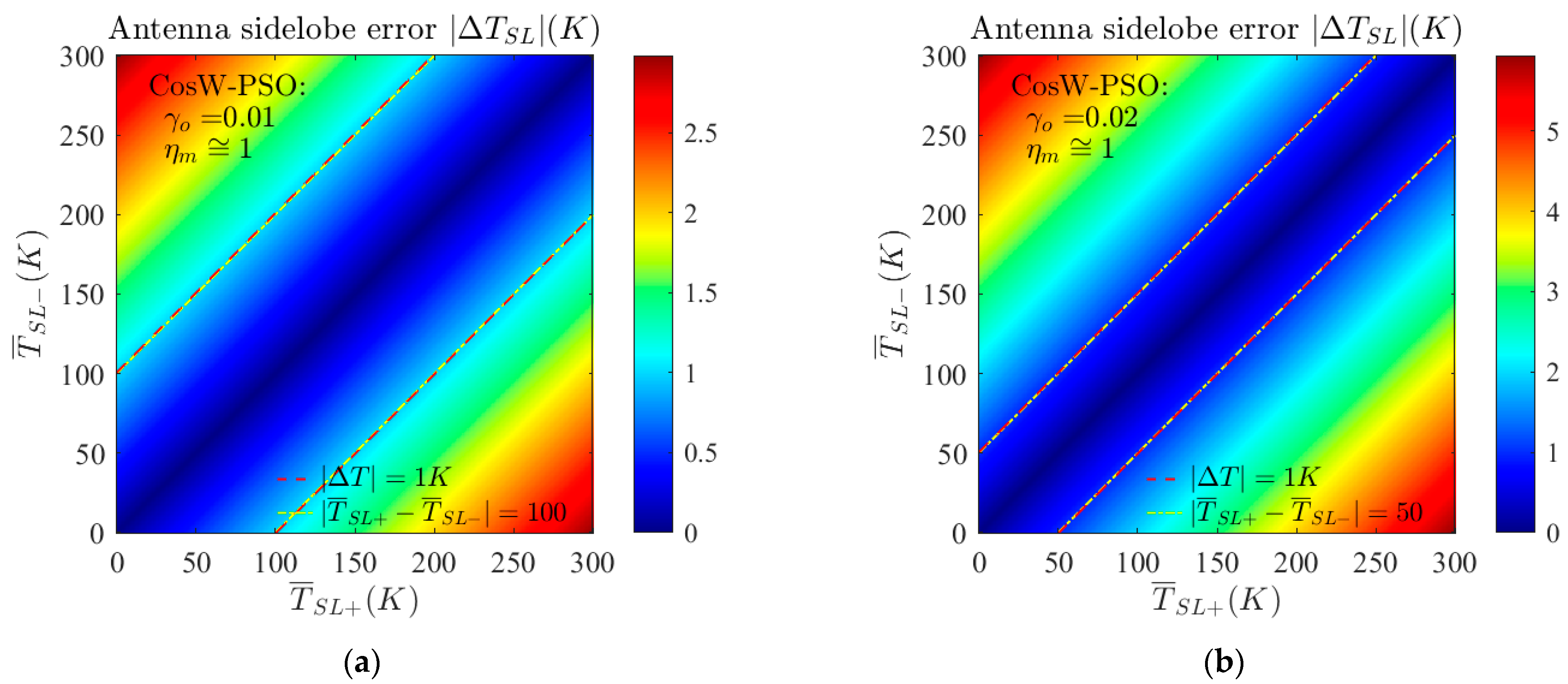
The variation in the sidelobe error with and for the product power patterns obtained by the CosW-PSO optimization for two values of is given in Figure 9. And is the newly defined main beam efficiency in [27]. Compared to Figure 4, the optimal solution of the sidelobe error of the optimized product power pattern coincides exactly with the line and has a value of 0 on this line. With the PSO optimization method, we can achieve the control and optimization of the sidelobe error by adjusting the value according to the average brightness temperature difference in the usage scenarios, thus improving the radiometer system performance.
4.2. Natural Scene Observation Simulation
When observing a natural scene, the positive and negative sidelobe mean brightness temperatures and change with the transition of the observed scene, and thus the sidelobe errors generated by antenna observations in different scenes will be different. The optimized antenna array product power pattern is used for natural scenario observation to verify its performance, and the observation results are compared with those of traditional weighted patterns.
The original scene image, shown in Figure 10, is a brightness temperature image of an estuarine coast, derived from optical remote sensing imagery with a pixel size of . Each irradiation of the antenna beam can obtain an observed bright temperature in the field of view located in the center region of the y-axis, and when the observation platform is moved along the x-dimension, the observation results of the scene temperature in the center strip (the region shown by the black dashed box in Figure 10) of the y-axis can be obtained.
The observed result here is the antenna temperature corresponding to (3), and the ideal measured temperature is the main lobe average brightness temperature obtained by irradiating the main beam alone. The sidelobe measurement errors generated by the antenna array are obtained by (8). It should be noted that here we are concerned with the measurement error caused by antenna sidelobe under different weighted window functions, rather than the difference between the antenna temperatures, because the angular resolutions of the antennas are significantly different at different weighted window functions, which will make their “ideal” temperature different.
Figure 11 shows the comparison of the Hanning window, Blackman window, and CosW-PSO optimized windows at and , as well as the corresponding Mills cross product power patterns on the . Then the weighted antenna array was, respectively, used to simulate the observation of the scene shown in Figure 10.
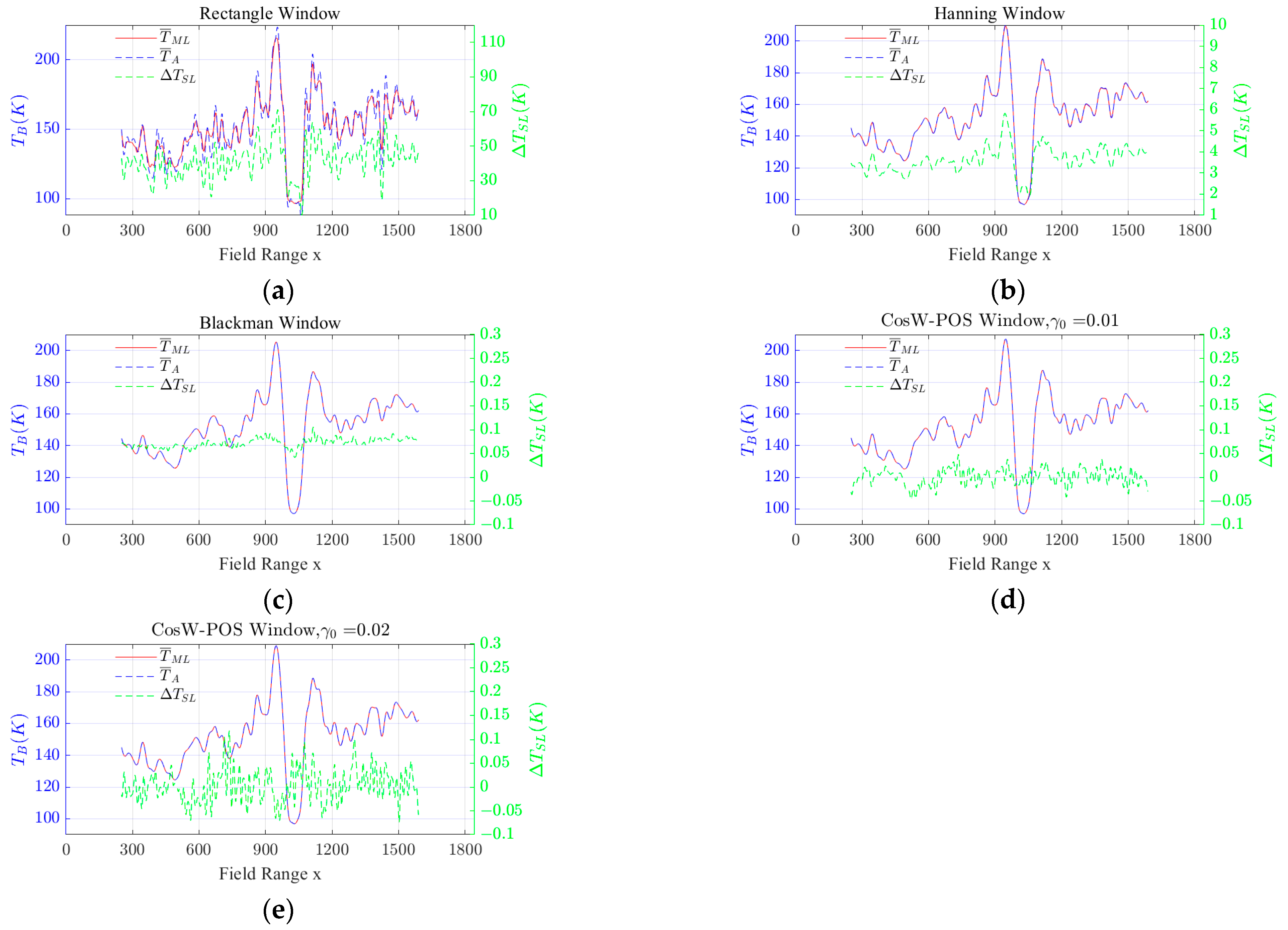
Observations of the brightness temperature of the strip in the center of the Y-axis at different weightings of the antenna array are given in Figure 12. The corresponding antenna array parameters are shown in Table 2. Figure 12a shows the numerical simulation results with rectangular windows, as a comparison, demonstrating the necessity of adding a window function to the Mills cross antenna array, otherwise, its sidelobes will introduce intolerable measurement errors.
When the Mills cross antenna array is under the Hanning window, the difference between positive and negative sidelobe solid angles is significant. As a result, the first term in (8) becomes the main influencing factor, leading to a large measurement error in antenna sidelobes during numerical simulations (Max() = 5.828 K), as shown in Figure 12b. This suggests that when the power pattern has negative sidelobes, the traditional window functions are no longer applicable and will introduce large measurement errors unless the SLL is suppressed to a very low level, such as the Blackman window, but this will result in a significant loss of spatial resolution.
As expected, the antenna array has better performance when the CosW-PSO optimized window function is applied, not only in terms of its reduction of the sidelobe error, but also in terms of its improvement in angular resolution (Table 2). As shown in Figure 12d, the CosW-PSO optimized window function with the sidelobe constraint improves the spatial resolution by 11% compared to the simulation results with the Blackman window, while the maximum measurement error due to the antenna sidelobe is reduced by half. Figure 12e relaxes the SLL requirement, , yet has a similar maximum sidelobe measurement error as the Blackman window, but with a 15.7% improvement in spatial resolution, which is comparable to the beamwidth as the Hanning window.
Numerical simulation results for natural scenarios demonstrate the improvement of Mills cross antenna performance by the CosW-PSO optimized window function. It is proved that the feasibility of using the positive and negative sidelobe received energy to cancel each other to reduce the effect of sidelobe error in radiometric measurements when there is a negative sidelobe in the antenna power pattern. This also benefits spatial resolution. It should also be mentioned that the optimization effect of the CosW-PSO window function will increase with the increase in array size. Because the larger the antenna array size, the more the number of sidelobes, so the distribution of positive and negative sidelobes will be closer and more uniform, resulting in the actual observation of the positive and negative sidelobes of the average brightness of the temperature difference being smaller, reducing the antenna sidelobe measurement error.
5. Conclusions
The correlation radiation measurement system based on the Mills cross array uses the coherence of the overlapping region of the cross beams and the multiplicative signal processing for radiometric measurements. This measurement mode produces deterioration in the sidelobe of the power pattern of the antenna array and the presence of negative sidelobes. On the one hand, a high sidelobe introduces a large sidelobe error, and therefore a windowing function of the antenna array is necessary. On the other hand, the “negative” energy received by the negative sidelobe cancels out the energy received by the positive sidelobe, reducing the overall energy leakage from the sidelobe. In this case, the measurement error caused by the sidelobes is affected by both the sidelobe level and the positive-to-negative sidelobe received energy ratio, which may result in a high sidelobe level but a small sidelobe error. This problem is illustrated in the article through the sidelobe characteristic analysis and numerical simulation of Mills cross array.
In this case, a weighting method based on the combined cosine window function algorithm and particle swarm optimization (CosW-PSO) is proposed for Mills cross array weighting. The theoretical analysis and simulation results demonstrate that this optimization method can make full use of the prior knowledge of the cosine window function and reduce the dimension of optimized particles to improve the convergence performance of the optimizer. Compared with the traditional PSO scheme, the window function generated by this method can inherit the excellent performance of the cosine window function and obtain the desired power pattern.
The simulation results of the natural scene show that the sidelobe energy leakage can be reduced by utilizing the cancellation of positive and negative sidelobes receiving energy from the Mills cross array. Additionally, the optimized CosW-PSO window function can improve the beam performance of the antenna array compared to conventional window functions. This is reflected in the fact that the CosW-PSO optimized window function has the least restriction on SLL for the same sidelobe error requirement, or that the use of the CosW-PSO optimized window function minimizes the sidelobe error uncertainty and improves the measurement accuracy for the same spatial resolution requirement.
Author Contributions
X.F. and H.L. proposed the concept and optimization model of CosW-PSO; X.F. and C.Z. established simulation models; X.F., D.H. and L.N. performed the simulation and analyzed the simulation results; D.H. funding; X.F. wrote the manuscript and H.L. edited this article. All authors have read and agreed to the published version of the manuscript.
Funding
This work is supported in part by the National Natural Science Foundation of China under Grant 42206185 and the National Space Science Center of CAS Foundation under Grant E2PD40017S.
Data Availability Statement
The data presented in this study are available on request from the corresponding author.
Conflicts of Interest
The authors declare no conflicts of interest.
References
- Mills, B.Y.; Little, A.G. A High-Resolution Aerial System of a New Type. Aust. J. Phys. 1953, 6, 272. [Google Scholar] [CrossRef]
- Milman, A.S. Sparse Aperture Microwave Radiometers for earth remote sensing. Radio Sci. 1988, 23, 193–205. [Google Scholar] [CrossRef]
- Shain, C.A. The Sydney 19.7-mc radio telescope. Proc. IRE 1958, 46, 85–88. [Google Scholar] [CrossRef]
- Mills, B.Y.; Little, A.G.; Sheridan, K.V.; Slee, O.B. A high resolution radio telescope for use at 3.5 m. Proc. IRE 1958, 46, 67–84. [Google Scholar] [CrossRef]
- Costian, C.H.; Lacey, J.D.; Roger, R.S. Large 22-MHz array for radio astronomy. IEEE Trans. Antennas Propag. 1969, 17, 162–169. [Google Scholar] [CrossRef]
- Malliot, H.A. A cross beam interferometer radiometer for high resolution microwave sensing. In Proceedings of the 1993 IEEE Aerospace Applications Conference Digest, Steamboat Springs, CO, USA, 31 January–5 February 1993; pp. 77–86. [Google Scholar]
- Grill, M.; Honary, F.; Nielsen, E.; Hagfors, T.; Dekoulis, G.; Chapman, P.; Yamagishi, H. A New Imaging Riometer based on Mills Cross Technique. In Proceedings of the 7th International Symposium on Communication Theory and Applications, Ambleside, UK, 13–18 July 2003; pp. 26–31. [Google Scholar]
- Li, Y.; Timms, G.P.; Archer, J.W.; Rosolen, G.C.; Tello, J.Y.; Brothers, M.L.; Hellicar, A.D.; Guo, Y.J. Passive millimeter-wave imaging using two scanning fan-beam antennas. In Proceedings SPIE—Passive Millimeter-Wave Imaging Technology X; SPIE: Bellingham, WA, USA, 2007; Volume 6548, pp. 65480E–65481E. [Google Scholar]
- Li, Y.; Archer, J.; Tello, J.; Rosolen, G.; Ceccato, F.; Hay, S.; Hellicar, A.; Guo, Y. Performance evaluation of a passive millimeter-wave imager. IEEE Trans. Microw. Theory Technol. 2009, 57, 2391–2405. [Google Scholar] [CrossRef]
- Verdilla, S.R. Calibration, Validation and Polarimetry in 2D Aperture Synthesis: Application to MIRAS. Ph.D. Thesis, University Politecnica de Catalunya, Barcelona, Spain, May 2005. [Google Scholar]
- Feng, X.; Liu, H.; Zhang, C.; Han, D.; Guo, X.; Niu, L. Performance Analysis of Cross Beam Correlation Microwave Radiometers Using Two Orthogonal Subarrays. IEEE Trans. Geosci. Remote Sens. 2024, 62, 5300717. [Google Scholar] [CrossRef]
- Grill, M. Technological Advances in Imaging Riometry. Ph.D. Thesis, University of Lancaster, Lancaster, UK, 2007. [Google Scholar]
- Bará, J.; Camps, A.; Torres, F.; Corbella, I. Angular resolution of two-dimensional, hexagonally sampled interferometric radiometers. Radio Sci. 1998, 33, 1459–1473. [Google Scholar] [CrossRef]
- Camps, A.; Corbella, I.; Bara, J.; Torres, F. Radiometric sensitivity computation in aperture synthesis interferometric radiometer. IEEE Trans. Geosci. Remote Sens. 1998, 36, 680–685. [Google Scholar] [CrossRef]
- Long, D.; Ulaby, F. Microwave Radar and Radiometric Remote Sensing; The University of Michigan Press: Ann Arbor, MI, USA, 2015. [Google Scholar]
- Kennedy, J.; Eberhart, R. Particle swarm optimization. Proc. IEEE Int. Conf. Neural Netw. 1995, 4, 1942–1948. [Google Scholar]
- Eberhart, R.C.; Kennedy, J. A new optimizer using particle swarm theory. In Proceedings of the Sixth International Symposium on Micromachine and Human Science, Nagoya, Japan, 4–6 October 1995; pp. 39–43. [Google Scholar]
- Jin, N.; Rahmat-Samii, Y. Advances in particle swarm optimization for antenna designs: Real-number, binary, single-objective and multiobjective implementations. IEEE Trans. Antennas Propag. 2007, 55, 556–567. [Google Scholar] [CrossRef]
- Jin, N.; Rahmat-Samii, Y. Analysis and particle swarm optimization of correlator antenna arrays for radio astronomy applications. IEEE Trans. Antennas Propag. 2008, 56, 1269–1279. [Google Scholar] [CrossRef]
- Khodier, M.M.; Christodoulou, C.G. Linear array geometry synthesis with minimum sidelobe level and null control using particle swarm optimization. IEEE Trans. Antennas Propag. 2008, 53, 1269–1279. [Google Scholar] [CrossRef]
- Gies, D.; Rahmat-Samii, Y. Particle swarm optimization for reconfigurable phased-differentiated array design. Microw. Opt. Technol. Lett. 2003, 38, 168–175. [Google Scholar] [CrossRef]
- Parsopoulos, K.; Vrahatis, M. Recent approaches to global optimization problems through particle swarm optimization. Nat. Comput. 2002, 1, 235–306. [Google Scholar] [CrossRef]
- Fieldsend, J.; Singh, S. A multi-objective algorithm based upon particle swarm optimization, an efficient data structure and turbulence. In Proceedings of the U.K. Workshop on Computational Intelligence, Birmingham, UK, 2–4 September 2002; pp. 37–44. [Google Scholar]
- Velduizen, D.; Zydallis, J.; Lamont, G. Considerations in engineering parallel multiobjective evolutionary optimizations. IEEE Trans. Evol. Comput. 2003, 7, 144–173. [Google Scholar] [CrossRef]
- Brown, A.D. Electronically Scanned Arrays-Matlab Modeling and Simulation; CRC Press, Taylor &. Francis Group, LLC: Boca Raton, FL, USA, 2012; pp. 35–80. [Google Scholar]
- Nuttall, A.H. Some windows with very good side lobe behavior. IEEE Trans. Acoust. Speech Signal Process. 1981, 29, 84–91. [Google Scholar] [CrossRef]
- Wu, J.; Zhang, C.; Liu, H.; Yan, J. Performance Analysis of Circular Antenna Array for Microwave Interferometric Radiometers. IEEE Trans. Geosci. Remote Sens 2017, 55, 3261–3271. [Google Scholar] [CrossRef]
Figure 1.
Observation model based on Mills cross antenna array.

Figure 2.
Mills cross antenna array. The and coordinates have been normalized by and .

Figure 3.
Amplitude and phase of product array factor of the 30 30 Mills cross array.

Figure 4.
Variation in with and , when the antenna array is added with (a) Hamming window, (b) Hanning window, and (c) Blackman window. The number of Mills cross array elements is set to 30 + 30, and the subarray element spacing is set to . Without loss of generality, the element pattern is replaced with normalized Gaussian functions.

Figure 5.
Particle swarm optimization flow diagram with the proposed strategy.

Figure 6.
Fitness values of two optimization strategies for (a) and (b) . The average global best of 10 independent trials increases the persuasiveness of the comparison.
Figure 6.
Fitness values of two optimization strategies for (a) and (b) . The average global best of 10 independent trials increases the persuasiveness of the comparison.

Figure 7.
The optimization window function of two optimization strategies when and .

Figure 8.
The amplitude and phase of the product power pattern weighted by (a) CosW-PSO and (b) Con-PSO optimized window functions when .
Figure 8.
The amplitude and phase of the product power pattern weighted by (a) CosW-PSO and (b) Con-PSO optimized window functions when .

Figure 9.
Variation in the sidelobe error with and for the product power patterns obtained by CosW-PSO optimization for (a) and (b) .
Figure 9.
Variation in the sidelobe error with and for the product power patterns obtained by CosW-PSO optimization for (a) and (b) .

Figure 10.
The brightness temperature distribution of the original scene used for numerical simulation. Obtained from optical remote sensing image of estuarine coast.
Figure 10.
The brightness temperature distribution of the original scene used for numerical simulation. Obtained from optical remote sensing image of estuarine coast.

Figure 11.
The window functions and corresponding array patterns used in numerical simulations.

Figure 12.
Antenna temperature and main lobe average brightness temperature as well as sidelobe error for the Mills cross antenna array with (a) rectangle window, (b) Hanning window, (c) Blackman window, and CosW-PSO optimization windows at (d) and (e) .
Figure 12.
Antenna temperature and main lobe average brightness temperature as well as sidelobe error for the Mills cross antenna array with (a) rectangle window, (b) Hanning window, (c) Blackman window, and CosW-PSO optimization windows at (d) and (e) .


Table 1.
Combined cosine window coefficients obtained by the CosW-PSO scheme.
| 0.01 | 0.3992 | 0.4976 | 0.0773 | 18.04 |
| 0.02 | 0.4450 | 0.5125 | 0.0551 | 17.93 |
Table 2.
Performance parameters and sidelobe errors of Mills cross antenna array with different window functions.
Table 2.
Performance parameters and sidelobe errors of Mills cross antenna array with different window functions.
| Rectangle | CosW-PSO | Blackman | Hanning | ||
|---|---|---|---|---|---|
| 3.2548 | 5.2731 | 5.0092 | 5.7951 | 5.0494 | |
| 0.7832 | 1 | 1 | 0.9995 | 0.9767 | |
| MSLL (dB) | −6.67 | −25.80 | −21.45 | −29.24 | −15.80 |
| \ | 0.01 | 0.02 | 0.003 | 0.015 | |
| \ | −0.01 | −0.02 | −0.002 | −0.039 | |
| Max () (K) | 71 | 0.052 | 0.118 | 0.106 | 5.828 |
| Mean () (K) | 41 | 0.0004 | 0.0028 | 0.0721 | 3.6234 |
1 MBE = computed by using the new definition in [27]. 2 and are the ratio of positive and negative sidelobe solid angles to the main lobe solid angles, respectively.
Disclaimer/Publisher’s Note: The statements, opinions and data contained in all publications are solely those of the individual author(s) and contributor(s) and not of MDPI and/or the editor(s). MDPI and/or the editor(s) disclaim responsibility for any injury to people or property resulting from any ideas, methods, instructions or products referred to in the content. |
© 2024 by the authors. Licensee MDPI, Basel, Switzerland. This article is an open access article distributed under the terms and conditions of the Creative Commons Attribution (CC BY) license (https://creativecommons.org/licenses/by/4.0/).
Share and Cite
MDPI and ACS Style
Feng, X.; Liu, H.; Zhang, C.; Han, D.; Niu, L. Improvement Method of Antenna Negative Sidelobes on Cross Beam Correlation Microwave Radiometer. Remote Sens. 2024, 16, 1245. https://doi.org/10.3390/rs16071245
AMA Style
Feng X, Liu H, Zhang C, Han D, Niu L. Improvement Method of Antenna Negative Sidelobes on Cross Beam Correlation Microwave Radiometer. Remote Sensing. 2024; 16(7):1245. https://doi.org/10.3390/rs16071245
Chicago/Turabian StyleFeng, Xiaolong, Hao Liu, Cheng Zhang, Donghao Han, and Lijie Niu. 2024. "Improvement Method of Antenna Negative Sidelobes on Cross Beam Correlation Microwave Radiometer" Remote Sensing 16, no. 7: 1245. https://doi.org/10.3390/rs16071245
Note that from the first issue of 2016, this journal uses article numbers instead of page numbers. See further details here.