Infrared Small Target Detection Based on Tensor Tree Decomposition and Self-Adaptive Local Prior

Abstract

Infrared small target detection plays a crucial role in both military and civilian systems. However, current detection methods face significant challenges in complex scenes, such as inaccurate background estimation, inability to distinguish targets from similar non-target points, and poor robustness across various scenes. To address these issues, this study presents a novel spatial–temporal tensor model for infrared small target detection. In our method, we introduce the tensor tree rank to capture global structure in a more balanced strategy, which helps achieve more accurate background estimation. Meanwhile, we design a novel self-adaptive local prior weight by evaluating the level of clutter and noise content in the image. It mitigates the imbalance between target enhancement and background suppression. Then, the spatial–temporal total variation (STTV) is used as a joint regularization term to help better remove noise and obtain better detection performance. Finally, the proposed model is efficiently solved by the alternating direction multiplier method (ADMM). Extensive experiments demonstrate that our method achieves superior detection performance when compared with other state-of-the-art methods in terms of target enhancement, background suppression, and robustness across various complex scenes. Furthermore, we conduct an ablation study to validate the effectiveness of each module in the proposed model.

1. Introduction

In comparison to active radar imaging, infrared imaging offers the benefits of enhanced portability and improved concealment. Meanwhile, compared with visible light systems, it boasts a range of advantages, such as exceptional anti-interference features and the ability to operate all throughout the day [1]. Owing to the superior benefits of infrared imaging, infrared dim and small target detection plays a significant role in military and civil applications, such as aerospace technology [2], security surveillance [3], and forest fire prevention [4]. However, due to the lengthy detection distance, infrared targets usually occupy only a few pixels and lack shape information and textural features. In addition, infrared images in complex scenes often contain a variety of interferences (e.g., heavy clutter and prominent suspicious targets), resulting in a weak signal-to-clutter ratio (SCR) [5]. Therefore, infrared small target detection remains a challenging issue and has attracted widespread research interests.

1.1. Related Works

In general, infrared small target detection algorithms primarily include single-frame detection and sequential-frame detection [6]. For a long time, many single-frame detection approaches have been developed to address the challenges in infrared small target detection. Single-frame detection methods can be divided into four categories: (1) background consistency-based methods; (2) human visual system (HVS)-based methods; (3) deep learning (DL)-based methods; and (4) low-rank and sparse decomposition (LRSD)-based methods.

• Background consistency-based methods achieve target enhancement and background suppression based on the assumption of background consistency. Typical methods include the Top-hat filter [7], Max–Mean and Max–Median filters [8], and the high-pass filter [9]. Hadhoud and Thomas [10] extended the LMS algorithm [11] and proposed a two-dimensional adaptive least mean square filter (TDLMS). Cao and Sun [12] utilized the maximum inter-class variance method to improve morphological filtering. Although these methods are capable of achieving fast detection speeds, they are unsuitable for application in complex scenes.
• Contrast is the most crucial factor encoded in our visual system; HVS-based methods generally utilize visual saliency features to distinguish the target from the background. Chen et al. [13] proposed a local contrast method (LCM) to describe the difference between the target and its neighborhood. Inspired by LCM, many methods based on local contrast improvement have been proposed. Starting from the perspective of image patch difference, Wei et al. [14] presented a multiscale patch-based contrast measure (MPCM). Shi et al. [15] proposed a high-boost-based multiscale local contrast measure (HBMLCM). Han et al. [16] designed a multiscale tri-layer local contrast measure (TLLCM) to compute comprehensive contrast. Han et al. [17] improved the detection accuracy by utilizing the Laplacian filter and proposed a coarse-to-fine structure (MCFS) for infrared small moving target detection. However, when the image contains background edges and pixel-sized noises with high brightness (PNHB), such algorithms usually display high false alarms.
• With the development of artificial neural networks, DL-based methods have received extensive attention for their application in infrared target detection. Fan et al. [18] improved the convolutional neural network to extract infrared image features, aiming to improve detection accuracy and efficiency. Zhao et al. [19] designed an architecture of generative adversarial network (GAN), which models the detection problem issue as an image-to-image translation problem. In [20], a novel Dim2Clear network (Dim2Clear) was proposed to solve the problem of noise interference. Recently, Ying et al. [21] developed a label evolution framework with single point supervision. Although DL-based methods can achieve good detection performance under training scenes, their generalization to practical applications remains a challenge.
• In recent years, LRSD-based methods have achieved great success and can now effectively separate the low rank background and the sparse target of infrared image. Gao et al. [22] first proposed an infrared patch-image model (IPI) by constructing local patches. Consequently, infrared small target detection is transformed into an optimization problem. However, as the nuclear norm minimization (NNM) uses the same threshold to shrink singular values, an over-shrinkage problem may occur in complex backgrounds full of interference [23]. Furthermore, besides the target, edges and corners in the background are also considered as sparse components under the $l_1$-norm [24]. To handle the above problems, Dai et al. [25] constructed a non-negative infrared patch-image model (NIPPS) by adding a non-negative constraint to the sparse target. Wang et al. [26] introduced the total variation regularization that better removes the noise and proposed a total variation regularization and principal component pursuit model (TV-PCP). Zhang et al. [27] designed a nonconvex rank approximation minimization (NRAM) by utilizing the $l_{\mathrm{2,1}}$-norm to constrain the remaining edges. Assuming that the background comes from multiple subspaces, the stable multi-subspace learning model (SMSL) [28] and the self-regularized weighted sparse model (SRWS) [29] were proposed to improve detection performance. In order to better extract the image structure information and meet the practical demand for fast detection speed, Dai and Wu [30] adopted the tensor structure and proposed a reweighted infrared patch-tensor model (RIPT). Zhang and Peng [31] combined the partial sum of the tensor nuclear norm (PSTNN) and the local prior to effectively improve detection efficiency. In [32], the tensor fibered nuclear norm based on the Log operator (LogTFNN) was used to nonconvex approximate the tensor rank, which helps suppress background and noise. Zhang et al. [33] constructed a non-local block tensor and an adaptive compromising factor based on the image local entropy. Then, a self-adaptive and non-local patch-tensor model (ANLPT) was proposed for infrared small target detection.

Although the above LRSD-based single-frame detection methods have achieved good results, they ignore temporal information. Traditional sequential-frame detection methods, such as 3D matched filtering [34], dynamic programming algorithms [35], the spatiotemporal saliency approach [36], and trajectory consistency [37], face challenges in effectively separating the background from the target. In addition, these methods usually require prior knowledge, which is difficult to obtain in practical applications. In order to exploit the spatial–temporal information that is neglected in LRSD-based single-frame detection approaches, Sun et al. [38] stacked images from successive adjacent frames. Inspired by this, Zhang et al. [39] proposed a novel spatial–temporal tensor model with edge-corner awareness to further improve detection ability. Considering that the Laplace operator can approximate the tensor rank more accurately, Hu et al. [40] proposed a multi-frame spatial–temporal patch-tensor model (MFSTPT). Wang et al. [41] integrated the nonoverlapping patch spatial–temporal tensor model (NPSTT) and the tensor capped nuclear norm (TCNN) for detection results with low false alarms. Further, Liu et al. [42] designed a nonconvex tensor Tucker decomposition method, in which factor prior was used to obtain accurate background estimation and reduce computational complexity.

1.2. Motivation

Compared with background consistency-based approaches and HVS-based approaches, low-rank and sparse tensor decomposition (LRSTD)-based methods can better enhance small target features and suppress background clutter interference. Among these approaches, single-frame detection methods only consider single-frame image to construct the optimization model and struggle to achieve accurate results in various challenging environments with dynamic change or heavy clutter. Considering the significance of combining contextual information in the spatial–temporal domain, this article primarily concentrates on sequential-frame infrared target detection. While currently available methods have achieved relatively good detection performance, there are still some issues that need to be addressed.

First, due to the complex multilinear structure of the tensor, the exact approximation of the background tensor rank is always a major difficulty. To improve the accuracy of background estimation, these LRSTD-based methods [30,31,43] focus on designing more accurate tensor rank constraints, such as the sum of nuclear norm (SNN), tensor nuclear norm (TNN), and tensor train nuclear norm. Nevertheless, it has been proven that SNN fails to accurately approximate the tensor rank [44]. According to the definition of TNN, it lacks flexibility and the ability to measure low-rankness from multiple modes [45]. Although tensor train rank has a well-balanced matricization scheme, it suffers from higher storage requirements [46]. In summary, the approximation of the background tensor rank still needs to be improved. Therefore, we apply tensor tree rank to separate target and background. Compared with the above strategies, tensor tree decomposition is a more balanced method that splits the modes of a tensor in a hierarchical way.

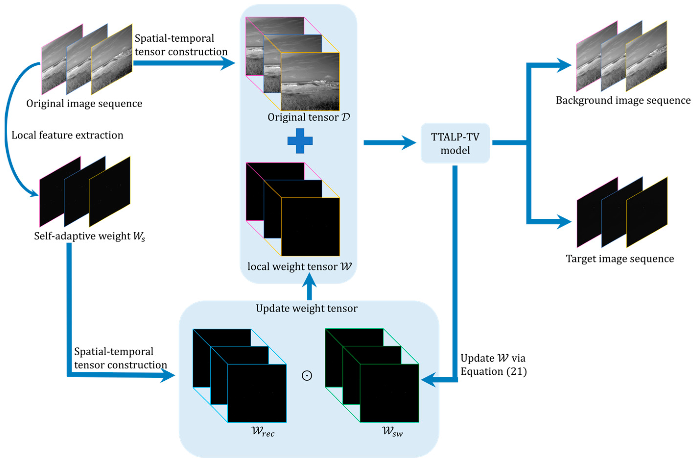
In addition to accurate background tensor estimation, the suppression of strong edges and corner points is key to achieving good detection performance. The local structure prior is often used to suppress interference. The RIPT only focuses on the edge structure information of the background, which may lead to false alarms. Likewise, the fixed prior weights used in PSTNN and MFSTPT cannot effectively suppress clutter in diverse scenes with different levels of interference. It is important to balance the enhancement of the target and the suppression of the interference from edges and corners in different scenes. To solve this problem, we propose a self-adaptive local prior method to adaptively suppress background clutter. Moreover, we use spatial–temporal total variation (STTV) to explore local smooth information. This strategy helps us to better remove the background noise. By combining tensor tree decomposition, self-adaptive local prior, and STTV, our method can accurately detect small targets. In the following sections, we refer to the proposed method as the TTALP-TV method. We present the results of qualitative and quantitative experiments to demonstrate that TTALP-TV surpasses other state-of-the-art methods in terms of target enhancement and background suppression in various complex scenes. Figure 1 presents the flowchart of our method. The main contributions of this article can be summarized as follows:

(1)

In order to approximate the tensor rank function more flexibly and accurately, we introduce tensor tree decomposition to exploit spatial and temporal correlation through a hierarchical structure.

(2)

The self-adaptive local prior is proposed as a target weight, which can not only better extract target information but also more effectively remove background clutter. Simultaneously, we impose STTV regularization constraint on the background to preserve image details and reduce noise interference.

(3)

We integrate the tensor tree rank, self-adaptive local prior, and STTV for infrared small target detection. An efficient optimization scheme using the alternating direction multiplier method (ADMM) is introduced to solve the proposed model.

The remaining sections of this article are organized as follows. Section 2 summarizes the notations and preliminaries of tensor tree decomposition. Section 3 introduces the TTALP-TV model and describes its optimization procedure in detail. In Section 4, we demonstrate the effectiveness of the proposed algorithm through extensive experiments and analyses. Finally, Section 5 concludes this article and discusses the future work.

2. Notations and Preliminaries

This section introduces the essential notations and preliminaries used in this research. In this paper, we use lowercase letters (e.g., $x$), boldface lowercase letters (e.g., $\mathbf{x}$), boldface capital letters (e.g., $X$), and Euler script (e.g., $\mathcal{X}$) to represent scalars, vectors, matrices, and tensors, respectively. The $D$th-order tensor $\mathcal{X}\in {\mathbb{R}}^{I_1\times \cdots \times I_D}$, and $\mathbb{D}=\left\{1,\cdots ,D\right\}$. The node-q tensor-matrix multiplication can be denoted as $\mathcal{Y}=\mathcal{X}{\times }_{q}U$, where $\mathcal{X}\in {\mathbb{R}}^{I_1\times \cdots \times I_D}$, $U\in {\mathbb{R}}^{J\times I_q}$, $\mathcal{Y}\in {\mathbb{R}}^{I_1\times \cdots \times I_{q-1}\times J\times I_{q+1}\times \cdots \times I_D}$, and q is the node in the tensor tree format.

The specific explanations of the symbols used are given in

Table 1. Mathematical symbols.

Notation	Explanation
$\mathcal{X}\in {\mathbb{R}}^{I_1\times I_2\times I_3}$	3th-order tensor
$\mathcal{X}(i,j,k$$)/x_{i,j,k}$	Its $(i,j,k$)-th element
$〈\mathcal{X},\mathcal{Y}〉$	The inner product of two tensors, ${\sum }_{i_1{,i}_{2,}{i}_3}{x}_{i_1{,i}_{2,}{i}_3}{y}_{i_1{,i}_{2,}{i}_3}$
${‖\mathcal{X}‖}_0$	The $l_0$-norm, the number of non-zero elements in $\mathcal{X}$
${‖\mathcal{X}‖}_1$	The $l_1$-norm, the sum of non-zero elements in $\mathcal{X}$
${‖\mathcal{X}‖}_F$	The Frobenius norm, the square root of the sum of the squares of all elements in $\mathcal{X}$
${‖X‖}_{*}$	The matrix nuclear norm, the sum of all singular values in $X$

.

Tensor Tree Network

Definition 1 (Tensor tree structure) [47].

For $D$th-order data, we define a binary tree $\mathbb{T}$ with root $\mathbb{D}$ as its dimension tree. Each node ${\mathbb{C}}_q\subset \mathbb{T},$ $q=1,\cdots ,Q$ possesses the following attributes:

• The node with only one entry is a leaf, i.e., ${\mathbb{C}}_p=\left\{d\right\}$. The set of all leaf nodes can be represented as follows:

$$\mathbb{F}(\mathbb{T})=\left\{{\mathbb{C}}_p\subset \mathbb{T} | {\mathbb{C}}_p \mathrm{i}\mathrm{s} \mathrm{a} \mathrm{l}\mathrm{e}\mathrm{a}\mathrm{f} \mathrm{n}\mathrm{o}\mathrm{d}\mathrm{e} \mathrm{o}\mathrm{f} \mathbb{T}, p=1,\cdots ,P\right\}$$

(1)

where $P$ is the number of leaves.

2.

The node consisting of two disjoint successors is an interior node. The set of all interior nodes is denoted by:

$$\mathbb{E}(\mathbb{T})=\mathbb{T}\setminus \mathbb{F}(\mathbb{T})$$

(2)

And $Q-P$ represents the number of interior nodes.

3.

The tree distance $h({\mathbb{C}}_q)$ is the distance between the node ${\mathbb{C}}_q\subset \mathbb{T}$ and the root, with a maximum depth of $H$. At depth $h$, $P_h$ and $Q_h$ denote the number of leaves and total nodes, respectively.

Definition 2 (Matricization) [47].

Given a node of dimension indices ${\mathbb{C}}_q\subset \mathbb{D}$ and its complement ${\overline{\mathbb{C}}}_q=\mathbb{D}\setminus {\mathbb{C}}_q$, the matricization of a tensor $\mathcal{X}\in {\mathbb{R}}^{I_1\times \cdots \times I_D}$ is defined as:

$$X_{\left[q\right]}\in {\mathbb{R}}^{I_{{\mathbb{C}}_q}\times I_{{\overline{\mathbb{C}}}_q}}$$

(3)

where $I_{{\mathbb{C}}_q}=\prod _{c\in {\mathbb{C}}_q}{I}_c$ and $I_{{\overline{\mathbb{C}}}_q}=\prod _{\overline{c}\in {\overline{\mathbb{C}}}_q}{I}_{\overline{c}}$.

Definition 3 (Tensor tree rank) [47].

Let $\mathbb{T}$ be a dimension tree of a $D$th-order tensor, the tensor tree rank is the set of ranks of the matricization for each node, in the form of:

$${\mathrm{r}\mathrm{a}\mathrm{n}\mathrm{k}}_{\mathrm{t}\mathrm{r}\mathrm{e}\mathrm{e}}=\left\{k_q|k_q=\mathrm{r}\mathrm{a}\mathrm{n}\mathrm{k}\left(X_{\left[q\right]}\right), \forall {\mathbb{C}}_q\subset \mathbb{T}\right\}$$

(4)

Definition 4 (Tensor tree decomposition) [47].

Given $\mathcal{X}\in {\mathbb{R}}^{I_1\times \cdots \times I_D}$, for every node ${\mathbb{C}}_q\subset \mathbb{T}$, $X_{\left[q\right]}$ can be written as:

$$X_{\left[q\right]}=U_q{V}_q^{\mathrm{T}}, U_q\subset {\mathbb{R}}^{I_{{\mathbb{C}}_q}\times k_{{\mathbb{C}}_q}}$$

(5)

where $k_{{\mathbb{C}}_q}$ is the standard matrix rank of $X_{\left[q\right]}$. For each ${\mathbb{C}}_q\subset \mathbb{E}(\mathbb{T})$ with two disjoint successors ${\mathbb{C}}_{q1}$ and ${\mathbb{C}}_{q2}$, the column vectors ${\mathbf{u}}_q\left(:,l\right)$ of $U_q$ can be expressed as:

$${\mathbf{u}}_q\left(:,l\right)=\sum _{l_1=1}^{k_{q_1}}\sum _{l_2=1}^{k_{q_2}}{\mathcal{G}}_q(l,l_1,l_2){\mathbf{u}}_{q_1}\left(:,l_1\right)⨂{\mathbf{u}}_{q_2}\left(:,l_2\right)$$

(6)

where ${\mathcal{G}}_q\left(l,l_1,l_2\right)$ is the coefficient of the linear combination. Figure 2 graphically illustrates the tensor tree decomposition of a 4th-order tensor, providing an intuitive understanding of its structure.

3. Methodology

3.1. Spatial–Temporal Infrared Tensor Model

According to the characteristic analysis in [22], the original infrared images can be linearly modeled as:

$$f_D=f_B+f_T+f_N$$

(7)

where $f_B$, $f_T$, $f_D$, and $f_N$ denote the background image, target image, infrared image, and noise image, respectively. Equation (7) only considers spatial data and ignores the target’s motion in the temporal dimension, increasing the risk of missed detections or false alarms in some complex infrared scenes. Moreover, compared with the matrix-based methods, in the tensor domain, we can explore the intrinsic relationships of the data from multiple perspectives and improve computational efficiency.

To ensure the comprehensive utilization of spatial and temporal information, we adopt the approach in [38] to construct spatial–temporal image tensor. As shown in Figure 1, the input image tensor $\mathcal{D}\in {\mathbb{R}}^{n_1\times n_2\times L}$ is constructed by stacking consecutive $L$ frames in chronological order from the infrared sequence. Therefore, Equation (7) is written as follows:

$$\mathcal{D}=\mathcal{B}+\mathcal{T}+\mathcal{N}$$

(8)

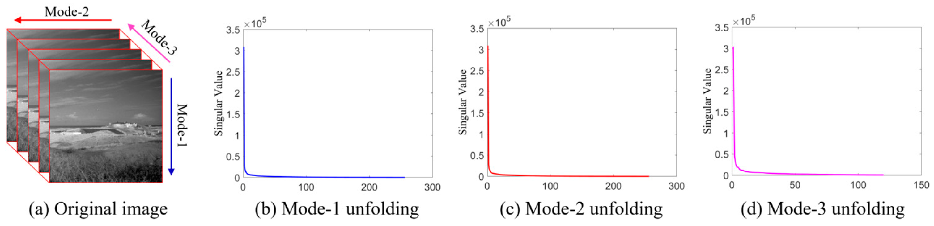
where $\mathcal{B}$, $\mathcal{T}$, $\mathcal{D},$ and $\mathcal{N}$ are the spatial–temporal tensor forms of $f_B$, $f_T$, $f_D$, and $f_N$, respectively. Figure 3 shows that the singular value distribution curves of the image tensor along mode 1, mode 2, and mode 3 rapidly decrease to zero. This indicates that background tensor $\mathcal{B}$ is a low-rank tensor. Given that the infrared small targets usually occupy only a few pixels in the entire image, it can be assumed that $\mathcal{T}$ is a sparse tensor. At the same time, it is commonly assumed that the noise in infrared images is additive Gaussian noise that satisfies ${‖\mathcal{N}‖}_F<\delta$. Therefore, the mathematical formula is as follows:

$$\begin{gathered} \underset{\mathcal{B},\mathcal{T}}{\min }\mathrm{r}\mathrm{a}\mathrm{n}\mathrm{k}(\mathcal{B})+{\lambda }_1{‖\mathcal{T}‖}_0 \\ \mathrm{s}.\mathrm{t}.{‖\mathcal{D}-\mathcal{B}-\mathcal{T}‖}_F<\delta \end{gathered}$$

(9)

where ${\lambda }_1$ is a positive regularization parameter balancing the trade-off between the target spatial–temporal tensor and the background spatial–temporal tensor. As the optimization of $l_0$-norm is NP-hard. In practice, it is usually substituted with the $l_1$-norm:

$$\begin{gathered} \underset{\mathcal{B},\mathcal{T}}{\min }\mathrm{r}\mathrm{a}\mathrm{n}\mathrm{k}(\mathcal{B})+{\lambda }_1{‖\mathcal{T}‖}_1 \\ \mathrm{s}.\mathrm{t}.{‖\mathcal{D}-\mathcal{B}-\mathcal{T}‖}_F<\delta \end{gathered}$$

(10)

3.2. Self-Adaptive Local Prior Information

In infrared images, the strong edges and corner points in the background exhibit sparsity similar to that of the target. This makes it difficult to completely distinguish them from the target when relying solely on global sparse features. Thus, it is essential to extract local prior and incorporate it into the optimization function to reduce background residuals. For this reason, the structure tensor [48] was used to depict the local geometry structure of infrared images. For an original infrared image $D$, the classic linear structure tensor can be calculated as follows:

$$J_{\rho }=K_{\rho }\ast \left(\nabla D_{\rho }⨂ \nabla D_{\rho }\right)=\left(\begin{array}{cc}{J}_{11}& J_{12}\\ J_{21}& J_{22}\end{array}\right)=\left(\begin{array}{cc}{K}_{\rho }\ast I_x^2& K_{\rho }\ast I_x{I}_y\\ K_{\rho }\ast I_x{I}_y& K_{\rho }\ast I_y^2\end{array}\right)$$

(11)

$$\begin{gathered} \lambda 1=\frac{1}{2}\left(J_{11}+J_{22}+\sqrt{{\left(J_{22}-J_{11}\right)}^2+4{J_{12}}^2}\right) \\ \lambda 2=\frac{1}{2}\left(J_{11}+J_{22}-\sqrt{{\left(J_{22}-J_{11}\right)}^2+4{J_{12}}^2}\right) \end{gathered}$$

(12)

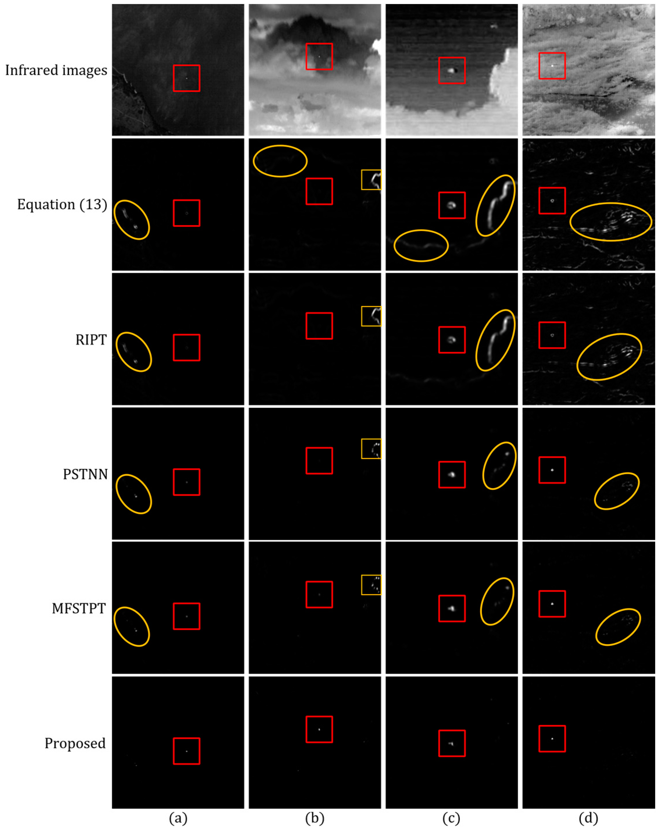
where $K_{\rho }$ denotes the Gaussian kernel function with variance $\rho$, $\ast$ denotes the convolution operation, $\nabla$ denotes the gradient, and $⨂$ denotes the Kronecker product. The difference between $\lambda 1$ and $\lambda 2$ reflects the image area to which the pixel belongs. When the pixel belongs to the flat region, $\lambda 1\approx \lambda 2\approx 0$; when the pixel belongs to the corner region, $\lambda 1\ge \lambda 2\gg 0$; and when the pixel belongs to the edge region, $\lambda 1\gg \lambda 2\approx 0$. The local prior information extracted in RIPT [30] is calculated as follows:

$$E\left(x,y\right)=\lambda 1-\lambda 2$$

(13)

where $\left(x,y\right)$ represents the pixel position. However, as shown in row 3 of Figure 4, RIPT only captures the edge structure information of the background, which may result in background residuals and the loss of targets. Brown et al. [49] proposed the following corner-strength function to highlight target information:

$$C\left(x,y\right)=\frac{\mathrm{d}\mathrm{e}\mathrm{t}\left(ST\left(x,y\right)\right)}{\mathrm{t}\mathrm{r}\left(ST\left(x,y\right)\right)}=\frac{\lambda 1\lambda 2}{\lambda 1+\lambda 2}$$

(14)

where $ST\left(·\right)$ means the structure tensor, and $\mathrm{d}\mathrm{e}\mathrm{t}\left(·\right)$ and $\mathrm{t}\mathrm{r}\left(·\right)$ represent the determinant and trace of the matrix, respectively. The PSTNN model [31] utilizes the maximum eigenvalue as the background weight function, rather than Equation (13), and combines it with Equation (14) to calculate the prior weight:

$$W_p\left(x,y\right)=C·E$$

(15)

Row 4 of Figure 4 shows that the PSTNN suppresses the residual edge effect to some extent, but there is still room for improvement. In MFSTPT model [40], a weighted geometric average strategy was developed to integrate edge weighting from Equation (13) and the corner-point weighting from Equation (14), which can be expressed as follows:

$$W_c\left(x,y\right)=\sqrt[n]{C^p·E^q}$$

(16)

However, as demonstrated in row 5 of Figure 4, strong edges are still not constrained effectively, despite the improved acquisition of target information. Based on the above analyses, we believe that the previous methods do not fully exploit the pixel information contained in $\lambda 1$ and $\lambda 2$. Another problem is that the weight-stretching parameter artificially set in RIPT and MFSTPT cannot effectively balance the enhancement of the target and the suppression of the background. The underlying reason is the lack of consideration of the clutter information content in infrared images across different scenes. Therefore, a self-adaptive local prior method is proposed to address the above issues. Inspired by the Frangi filter [50], we utilize the ratio and the difference of eigenvalues to highlight target information and suppress background interference:

$$\begin{gathered} R\left(x,y\right)=\frac{\left|\lambda 1\right|}{\left|\lambda 2\right|} \\ \beta =\mathrm{m}\mathrm{e}\mathrm{a}\mathrm{n}\left(\sqrt[3]{\lambda 1-\lambda 2}\right) \end{gathered}$$

(17)

where $R\left(x,y\right)$ represents the statistical measure of edges and corner points, and $\left|\lambda 1\right|>\left|\lambda 2\right|$. In edge and corner-point regions, a larger difference between the eigenvalues results in a higher $R$-value. In contrast, in flat regions, the similarity between the two eigenvalues leads to a lower $R$-value. In addition, the $\beta$-value reflects the level of background interference contained in the original image. In scenes with strong clutter, the $\beta$-value is larger. Instead, as the background clutter decreases, the $\beta$-value will also be smaller. This can be used to adaptively suppress edges and corners. Thus, the final self-adaptive prior weight is described as:

$$W_s\left(x,y\right)=\mathrm{e}\mathrm{x}\mathrm{p}\left(-\frac{R^2}{2\beta }\right)·\left(1-\mathrm{e}\mathrm{x}\mathrm{p}\left(-\frac{{\lambda 1}^2+{\lambda 2}^2}{2c^2}\right)\right)$$

(18)

where $c$ denotes the half of the maximum of $\sqrt{{\lambda 1}^2+{\lambda 2}^2}$. The last row in Figure 4 shows that the proposed self-adaptive weight effectively suppresses the residual effect of strong edges and bright corner points, while also highlighting the target information. It can be seen that the adaptive factor $\beta$ enhances suppression in scenes with strong clutter, resulting in a slight target shrinkage, but significantly reduces background residuals compared to other methods. Then, we construct the spatial–temporal tensor ${\mathcal{W}}_s$ and normalize it as follows:

$${\mathcal{W}}_s=\frac{{\mathcal{W}}_s-w_{min}}{w_{max}-w_{min}}$$

(19)

where $w_{max}$ and $w_{min}$ denote the maximum and minimum values of ${\mathcal{W}}_s$, respectively. In order to accelerate the convergence speed and improve the computational efficiency, we use the reweighted scheme [51] to add a sparse weight:

$${\mathcal{W}}_{sw}^{k+1}=\frac{c}{\left|{\mathcal{T}}^k\right|+\epsilon }$$

(20)

where $c$ denotes a non-negative constant, $\epsilon$ represents a small positive number preventing the denominator from being 0, and $k$ is the number of iterations. Considering that self-adaptive prior weight in Equation (19) can suppress edges and corner points, we obtain ${\mathcal{W}}_{rec}$ by taking the reciprocal of the corresponding elements in ${\mathcal{W}}_s$. Combined with the sparse weight in Equation (20), we build the final local prior tensor as follows:

$$\mathcal{W}={\mathcal{W}}_{rec}\odot {\mathcal{W}}_{sw}$$

(21)

where $\odot$ represents the Hadamard product.

3.3. Spatial–Temporal Total Variation Regularization

In real-world infrared scenes, heavy noise can be a significant interference, causing false alarms in target detection. Fortunately, the TV model effectively reduces image noise while simultaneously preserving the spatial piecewise smoothness. Introduced by Rudin [52], TV regularization can distinguish between areas with significant variations, such as edges and textures, and smooth areas with large amounts of noise. For the matrix $X\in {\mathbb{R}}^{I_1\times I_2}$, the TV norm can be mathematically expressed as follows:

$$\begin{gathered} {‖X‖}_{\mathrm{T}\mathrm{V}}=\sum _{i=1}^{I_1-1}\sum _{j=1}^{I_2-1}\left(\left|X_{i+1,j}{-X}_{i,j}\right|+\left|{X_{i,j+1}-X}_{i,j}\right|\right) \\ +\sum _{i=1}^{I_1-1}\left|{X_{i+1,I_2}-X}_{i,I_2}\right|+\sum _{j=1}^{I_2-1}\left|{X_{I_1,j+1}-X}_{I_1,j}\right| \end{gathered}$$

(22)

It can be seen from Equation (22) that the matrix-based TV framework only depicts the spatial continuity of the infrared targets and ignores the temporal continuity between successive frames. For the exploration of temporal coherence and spatio-temporal smoothing of small targets, the STTV can be obtained:

$${‖\mathcal{X}‖}_{\mathrm{S}\mathrm{T}\mathrm{T}\mathrm{V}}={‖D_h\mathcal{X}‖}_1+{‖D_v\mathcal{X}‖}_1+{‖D_z\mathcal{X}‖}_1$$

(23)

$$D_h\mathcal{X}=\mathcal{X}\left(i+1,j,k\right)-\mathcal{X}\left(i,j,k\right)$$

(24)

$$D_v\mathcal{X}=\left(\mathcal{X}|i,j+1,k\right)-\mathcal{X}\left(i,j,k\right)$$

(25)

$$D_z\mathcal{X}=\mathcal{X}\left(i,j,k+1\right)-\mathcal{X}\left(i,j,k\right)$$

(26)

where $D_h$, $D_v$, and $D_z$ represent the horizontal, vertical, and temporal difference operators, respectively. This spatiotemporal form of TV can be seen as an effective regular item, and it exhibits a degree of resilience against noise while preserving the image details. Furthermore, it not only emphasizes the spatial smoothness of the local region in the image but also considers that the target remains temporally consistent among successive frames.

3.4. The Proposed TTALP-TV Model

In tensor robust principal component analysis (TRPCA) problems, the rank function is a nonconvex objective to solve. Therefore, the approximation of low-rank background tensor $\mathcal{B}$ in Formula (10) is a crucial issue. A recent study [53] shows that employing the tensor tree-based TRPCA method can measure low-rankness of each mode and reduce memory requirements. In this article, we leverage the advantages of tensor tree rank and present the following optimization model:

$$\begin{gathered} \underset{\mathcal{B},\mathcal{T}}{\min }{{\mathbf{w}}^T\mathrm{r}\mathrm{a}\mathrm{n}\mathrm{k}}_{\mathrm{t}\mathrm{r}\mathrm{e}\mathrm{e}}\left(\mathcal{B}\right)+{\lambda }_1{‖\mathcal{T}‖}_1 \\ \mathrm{s}.\mathrm{t}.{‖\mathcal{D}-\mathcal{B}-\mathcal{T}‖}_F<\delta \end{gathered}$$

(27)

where ${\mathrm{r}\mathrm{a}\mathrm{n}\mathrm{k}}_{\mathrm{t}\mathrm{r}\mathrm{e}\mathrm{e}}\left(\mathcal{B}\right)={\left[k_1,\cdots ,k_Q\right]}^T$ is the tensor tree rank and the weighting vector ${\mathbf{w}}^T$ meets ${\sum }_{q=1}^Q{w}_q=1$. The direct minimization of tensor tree ranks in Formula (27) is NP-hard. As such, we can use their matrix nuclear norms as convex surrogates:

$$\begin{gathered} \underset{\mathcal{B},\mathcal{T}}{\min }\sum _{q=1}^Q{w}_q{‖B_{\left[q\right]}‖}_{\ast }+{\lambda }_1{‖\mathcal{T}‖}_1 \\ \mathrm{s}.\mathrm{t}.{‖\mathcal{D}-\mathcal{B}-\mathcal{T}‖}_F<\delta \end{gathered}$$

(28)

Furthermore, we incorporate the local prior tensor and STTV regularization to obtain the prior information and suppress background noise, respectively. The proposed TTALP-TV model is as follows:

$$\begin{gathered} \underset{\mathcal{B},\mathcal{T}}{\min }\sum _{q=1}^Q{w}_q{‖B_{\left[q\right]}‖}_{\ast }+{\lambda }_1{‖\mathcal{W}\odot \mathcal{T}‖}_1+{\lambda }_2{‖\mathcal{B}‖}_{\mathrm{S}\mathrm{T}\mathrm{T}\mathrm{V}} \\ \mathrm{s}.\mathrm{t}.{‖\mathcal{D}-\mathcal{B}-\mathcal{T}‖}_F<\delta \end{gathered}$$

(29)

where ${\lambda }_2$ is a positive regularization parameter.

3.5. Optimization Procedure

The objective function (29) can be solved effectively using the ADMM [54] method. By introducing four auxiliary variables, $\mathcal{X}$, $Z_1$, $Z_2$, and $Z_3,$ we obtain the following model:

$$\begin{gathered} \underset{\mathcal{B},\mathcal{T}}{\min }\sum _{q=1}^Q{w}_q{‖X_{\left[q\right]}‖}_{\ast }+{\lambda }_1{‖\mathcal{W}\odot \mathcal{T}‖}_1+{\lambda }_2\left({‖Z_1‖}_1+{‖Z_2‖}_1+{‖Z_3‖}_1\right) \\ \mathrm{s}.\mathrm{t}.{‖\mathcal{D}-\mathcal{B}-\mathcal{T}‖}_F<\delta ,\mathcal{X}=\mathcal{B},{ Z}_1=D_h\mathcal{B},{ Z}_2=D_v\mathcal{B},{ Z}_3=D_z\mathcal{B} \end{gathered}$$

(30)

Based on the inexact augmented Lagrangian multiplier (IALM) [55], Equation (30) is written as:

$$\begin{gathered} L_A\left(\mathcal{B},\mathcal{T},\mathcal{X},Z\right)=\sum _{q=1}^Q{w}_q{‖X_{\left[q\right]}‖}_{\ast }+{\lambda }_1{‖\mathcal{W}\odot \mathcal{T}‖}_1+{\lambda }_2\left({‖Z_1‖}_1+{‖Z_2‖}_1+{‖Z_3‖}_1\right) \\ +\langle y_1,\mathcal{D}-\mathcal{B}-\mathcal{T}\rangle +〈y_2,\mathcal{X}-\mathcal{B}〉+〈y_3,{ Z}_1-D_h\mathcal{B}〉 \\ +〈y_4,{ Z}_2-D_v\mathcal{B}〉+〈y_5,{ Z}_3-D_z\mathcal{B}〉+\frac{\mu }{2}({‖\mathcal{D}-\mathcal{B}-\mathcal{T}‖}_F^2 \\ +{‖\mathcal{X}-\mathcal{B}‖}_F^2+{‖{ Z}_1-D_h\mathcal{B}‖}_F^2+{‖{ Z}_2-D_v\mathcal{B}‖}_F^2+{‖{ Z}_3-D_z\mathcal{B}‖}_F^2) \end{gathered}$$

(31)

where $y_1,y_2,y_3,y_4, \mathrm{a}\mathrm{n}\mathrm{d} y_5$ are the Lagrangian multipliers, and $\mu$ represents a positive penalty parameter. Using the ADMM framework, we can divide the Equation (31) into the following subproblems:

(a)

Updating $\mathcal{X}$ with other variables being fixed:

$$\begin{gathered} \mathcal{X}=\underset{\mathcal{X}}{\mathrm{arg\; min}}\sum _{q=1}^Q{w}_q{‖X_{\left[q\right]}‖}_{\ast }+〈y_2,\mathcal{X}-\mathcal{B}〉+\frac{\mu }{2}{‖\mathcal{X}-\mathcal{B}‖}_F^2 \\ \underset{\mathcal{X}}{=\mathrm{arg\; min}}\sum _{q=1}^Q{w}_q{‖X_{\left[q\right]}‖}_{\ast }+\frac{\mu }{2}{‖\mathcal{X}-\left(\mathcal{B}-\frac{y_2}{\mu }\right)‖}_F^2 \end{gathered}$$

(32)

Let $\tau =\frac{w_q}{\mu }$ and $\mathcal{S}=\mathcal{B}-\frac{y_2}{\mu }$, Equation (32) can be rewritten as:

$$\mathcal{X}=\underset{\mathcal{X}}{\mathrm{arg\; min}}\sum _{q=1}^Q\tau {‖X_{\left[q\right]}‖}_{\ast }+\frac{1}{2}{‖X_{\left[q\right]}-S_{\left[q\right]}‖}_F^2$$

(33)

For each node ${\mathbb{C}}_q\subset \mathbb{T}$, the solution of $X_{\left[q\right]}$ can be obtained by the singular value thresholding (SVT) [56]:

$$X_{\left[q\right]}={\mathrm{S}\mathrm{V}\mathrm{T}}_{\tau }\left(S_{\left[q\right]}\right)=U{\mathrm{s}\mathrm{t}\mathrm{h}}_{\tau }\left(\sum \right)V^{\mathrm{H}}$$

(34)

where ${\mathrm{s}\mathrm{t}\mathrm{h}}_{\tau }\left(s\right)=\mathrm{s}\mathrm{g}\mathrm{n}\left(s\right)\mathrm{m}\mathrm{a}\mathrm{x}(\left|s\right|-\tau ,0)$ and $\mathrm{H}$ denotes the complex conjugate.

According to the tensor tree structure of $\mathcal{X}$, $U_q$ can be used to represent the updated node value instead of directly updating $X_{\left[q\right]}$. Moreover, after updating the two successor nodes ${\mathbb{C}}_{q_1},{\mathbb{C}}_{q_2}\subset {\mathbb{C}}_q$, we can update the transfer tensor ${\mathcal{G}}_q$ to represent $U_q$ for each interior node ${\mathbb{C}}_q\subset \mathbb{T}$, where ${\mathcal{G}}_q$ is obtained by applying SVT to the new tensor $\mathcal{C}=\mathcal{S}{\times }_{q_1}{U}_{q_1}{\times }_{q_2}{U}_{q_2}$. In summary, we can utilize tensor tree decomposition to update $\mathcal{X}$, and the solution details are summarized in Algorithm 1.

Algorithm 1: The updating of $\mathcal{X}$ from leaves to roots.

Input: $\mathcal{S}$, $\tau$

for $p=1,\cdots , P$

$\left[U_p,k_p\right]={\mathrm{S}\mathrm{V}\mathrm{T}}_{\tau }\left(S_{\left[p\right]}\right)$   end for ${\mathcal{C}}_{H-1}=\mathcal{S}{\times }_1{U}_1{\times }_2{U}_2\cdots {\times }_P{U}_P$

for $h=H-1,\cdots , 0$ do

for $q_h=1,\cdots , Q_h$ do     if (the $q_h$ node is an interior one)       $\left[{\widehat{U}}_{q_h},{\widehat{k}}_{q_h}\right]={\mathrm{S}\mathrm{V}\mathrm{T}}_{{\tau }_{q_h}}\left(C_{\left[q_h\right]}\right)$       ${\mathcal{G}}_{q_h}=\mathrm{r}\mathrm{e}\mathrm{s}\mathrm{h}\mathrm{a}\mathrm{p}\mathrm{e}\left({\widehat{U}}_{q_h},{\widehat{k}}_{q_h}, {\widehat{k}}_{q_{h,1}},{\widehat{k}}_{q_{h,2}} \right)$     end if   end for   ${\mathcal{C}}_{h-1}={\mathcal{C}}_h{\times }_1{\widehat{U}}_1{\times }_2{\widehat{U}}_2\cdots {\times }_{(Q_h-P_h)}{\widehat{U}}_{(Q_h-P_h)}$

end for $\mathcal{X}$ can be constructed from ${\mathcal{G}}_q$ and $U_q$

Output: $\mathcal{X}$

(b)

Updating $\mathcal{B}$ with other variables being fixed:

$$\begin{gathered} \mathcal{B}=\underset{\mathcal{B}}{\mathrm{arg\; min}}\frac{\mu }{2}({‖\mathcal{D}-\mathcal{B}-\mathcal{T}+\frac{y_1}{\mu }‖}_F^2+{‖\mathcal{X}-\mathcal{B}+\frac{y_2}{\mu }‖}_F^2 \\ \hspace{1em}\hspace{1em}\hspace{1em}\hspace{1em}\hspace{1em}\hspace{1em}\hspace{1em}\hspace{1em}+{‖{ Z}_1-D_h\mathcal{B}+\frac{y_3}{\mu }‖}_F^2+{‖{ Z}_2-D_v\mathcal{B}+\frac{y_4}{\mu }‖}_F^2+{‖{ Z}_3-D_z\mathcal{B}+\frac{y_5}{\mu }‖}_F^2) \end{gathered}$$

(35)

The closed form solution of Equation (35) is expressed as follows:

$$\mathcal{B}={\mathcal{F}}^{-1}\left(\frac{\mathcal{F}\left(L+{\theta }_1+{\theta }_2+{\theta }_3\right)}{2+{\sum }_{i\in \left\{h,v,z\right\}}\mathcal{F}{\left(D_i\right)}^{\mathrm{H}}\mathcal{F}\left(D_i\right)}\right)$$

(36)

where $L=\mathcal{D}-\mathcal{T}+\mathcal{X}+\left(y_1∕\mu \right)+\left(y_2∕\mu \right)$, ${\theta }_1=D_h^{\mathrm{T}}\left(Z_1+\left(y_3∕\mu \right)\right)$, ${\theta }_2=D_v^{\mathrm{T}}\left(Z_2+\left(y_4∕\mu \right)\right)$, and ${\theta }_3=D_z^{\mathrm{T}}\left(Z_3+\left(y_5∕\mu \right)\right)$. $\mathcal{F}$ and ${\mathcal{F}}^{-1}$ represent the fast nFFT operator and the inverse nFFT operator, respectively.

(c)

Updating $\mathcal{T}$ with other variables being fixed:

$$\mathcal{T}=\underset{\mathcal{T}}{\mathrm{arg\; min}}{\lambda }_1{‖\mathcal{W}\odot \mathcal{T}‖}_1+\frac{\mu }{2}{‖\mathcal{D}-\mathcal{B}-\mathcal{T}+\frac{y_1}{\mu }‖}_F^2$$

(37)

Using the element-wise shrinkage approach [57], $\mathcal{T}$ is updated by:

$$\mathcal{T}={\mathrm{T}\mathrm{H}}_{\frac{{\lambda }_1}{\mu }}\left(\mathcal{D}-\mathcal{B}+\frac{y_1}{\mu }\right)$$

(38)

where $\mathrm{T}\mathrm{H}\left(·\right)$ denotes the element-wise shrinkage operator.

(d)

Updating $Z_1$, $Z_2$, ${\mathrm{a}\mathrm{n}\mathrm{d} Z}_3$ with other variables being fixed:

$$\left\{\begin{array}{c}{ Z}_1=\underset{{\mathit{Z}}_1}{\mathrm{arg\; min}}{\lambda }_2{‖Z_1‖}_1+\frac{\mu }{2}{‖{ Z}_1-D_h\mathcal{B}+\frac{y_3}{\mu }‖}_F^2\\ { Z}_2=\underset{{\mathit{Z}}_2}{\mathrm{arg\; min}}{\lambda }_2{‖Z_2‖}_1+\frac{\mu }{2}{‖{ Z}_2-D_v\mathcal{B}+\frac{y_4}{\mu }‖}_F^2\\ { Z}_3=\underset{{\mathit{Z}}_3}{\mathrm{arg\; min}}{\lambda }_2{‖Z_3‖}_1+\frac{\mu }{2}{‖{ Z}_3-D_z\mathcal{B}+\frac{y_5}{\mu }‖}_F^2\end{array}\right.$$

(39)

The Equation (39) can be solved by the element-wise shrinkage operator:

$$\left\{\begin{array}{c}{ Z}_1={\mathrm{T}\mathrm{H}}_{\frac{{\lambda }_2}{\mu }}\left(D_h\mathcal{B}-\frac{y_3}{\mu }\right)\\ { Z}_2={\mathrm{T}\mathrm{H}}_{\frac{{\lambda }_2}{\mu }}\left(D_v\mathcal{B}-\frac{y_4}{\mu }\right)\\ { Z}_3={\mathrm{T}\mathrm{H}}_{\frac{{\lambda }_2}{\mu }}\left(D_z\mathcal{B}-\frac{y_5}{\mu }\right)\end{array}\right.$$

(40)

(e)

Updating Lagrangian multipliers $y_1,y_2,y_3,y_4,\mathrm{a}\mathrm{n}\mathrm{d} y_5$ with other variables being fixed:

$$\left\{\begin{array}{c}{y}_1=y_1+\mu \left(\mathcal{D}-\mathcal{B}-\mathcal{T}\right)\\ y_2=y_2+\mu \left(\mathcal{X}-\mathcal{B}\right)\\ y_3=y_3+\mu \left(Z_1-D_h\mathcal{B}\right)\\ y_4=y_4+\mu \left(Z_2-D_v\mathcal{B}\right)\\ y_5=y_5+\mu \left(Z_3-D_z\mathcal{B}\right)\end{array}\right.$$

(41)

(f)

Updating penalty parameter $\mu$ by $\mu =\mathrm{m}\mathrm{i}\mathrm{n}\left(\rho \mu ,{\mu }_{\mathrm{m}\mathrm{a}\mathrm{x}}\right)$.

The complete process of the ADMM optimization method is given in Algorithm 2.

Algorithm 2: TTALP-TV algorithm

Input: The spatial–temporal tensor $\mathcal{D}\in {\mathbb{R}}^{n_1\times n_2\times L},$ $\mathrm{parameters} {\lambda }_1,$ ${\lambda }_2,$ $\mu$

Initialize: ${\mathcal{B}}^0=\mathcal{D},$ ${\mathcal{T}}^0=Z_i^0=0,$ $i=1, 2, 3,$ $y_i^0=0,$ $i=1, 2, 3, 4, 5,$ ${\mu }^0=5\mathrm{e}-3,$ ${\mu }_{\mathrm{m}\mathrm{a}\mathrm{x}}=1\mathrm{e}6,$ $\rho =1.2$$, \zeta =1e-6$$, \mathrm{maximum} \mathrm{iteration} \mathrm{step} K=100$.

While not converged do

1: $\mathrm{Update} {\mathcal{X}}^{k+1}$ by Algorithm 1

2: $\mathrm{Update} {\mathcal{B}}^{k+1}$ via Equation (36)

3: $\mathrm{Update} {\mathcal{T}}^{k+1}$ via Equation (38) 4: $\mathrm{Update} {\mathcal{W}}^{k+1}$ via Equation (21)

5: $\mathrm{Update} {{ Z}_1}^{k+1}, {{ Z}_2}^{k+1}, {{ Z}_3}^{k+1}$ via Equation (40)

6: Update Lagrangian multipliers $y_i^{k+1},$$i=1, 2, 3, 4, 5$ via Equation (41)

7: $\mathrm{Update} \mathrm{penalty} \mathrm{parameter} \mu$ via                  $\mu =\mathrm{m}\mathrm{i}\mathrm{n}\left(\rho \mu ,{\mu }_{\mathrm{m}\mathrm{a}\mathrm{x}}\right)$

8: Check the convergence condition                $\frac{{‖\mathcal{D}-{\mathcal{B}}^{k+1}-{\mathcal{T}}^{k+1}‖}_F^2}{{‖\mathcal{D}‖}_F^2}\le \zeta$

9: $\mathrm{Update} k=k+1$

End while

Output: Background component $\mathcal{B}$ and target component $\mathcal{T}$.

3.6. Steps of Detection Method

Figure 1 elaborates the whole process of the proposed TTALP-TV model, which is described as follows:

• Self-adaptive local prior extraction. Given an infrared image, the self-adaptive prior weight $W_s$ is calculated by Equation (18).
• Spatial–temporal tensor construction. The spatial–temporal infrared tensor $\mathcal{D}\in {\mathbb{R}}^{n_1\times n_2\times L}$ and local prior tensor $\mathcal{W}\in {\mathbb{R}}^{n_1\times n_2\times L}$ are constructed by stacking consecutive $L$ frames in chronological order from the original image sequence and the prior weight map, respectively.
• Background and target separation. The spatial–temporal infrared tensor $\mathcal{D}$ is decomposed into background tensor $\mathcal{B}$ and target tensor $\mathcal{T}$ through Algorithm 2.

Image reconstruction. Contrary to the construction process, the target image $f_T$ is reconstructed from $\mathcal{T}$.

4. Experimental Results

In this section, we first discuss the datasets used in infrared target detection experiments. Then, we introduce evaluation metrics and analyze the effects of several important parameters on the TTALP-TV model. Finally, we evaluate the detection ability and robustness of the proposed algorithm and compare it with eight state-of-the-art methods in six complex scenes.

4.1. Experiment Data

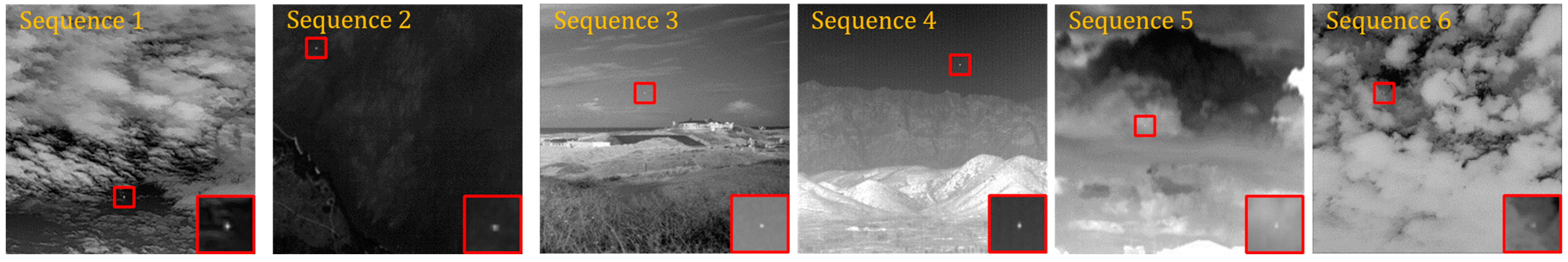
The dataset used in the experiments consists of six infrared image sequences, including complex scenes such as sky, sea, clouds, mountains, and buildings. The infrared sequences 1, 3, 4, and 6 are from [58,59]. In order to carry out an objective assessment of TTALP-TV from diverse scenes, we simulated infrared sequences 2 and 5 using the strategy in [22]. As shown in Figure 5, the images are uniformly scaled to the same size to improve target visibility. Meanwhile, each small target is marked by a red rectangle and magnified in the bottom right corner of the image. It can be seen that, in most scenes, the targets occupy a few pixels and lack shape information and texture features. Due to heavy clutter interference in complex scenes, it is difficult to distinguish the target from the background. The specific descriptions of sequences are presented in

Table 2. Characteristics of the dataset.

Sequence	Frames	Image Size	Target Descriptions	Background Descriptions
1	120	$256\times 256$	Slow-moving and small	Ground background with fierce clouds and noise
2	120	$256\times 256$	Slow-moving and weak airplane	Ground background with sea and islands
3	120	$256\times 256$	Fast-moving, small and dim	Ground background with bright buildings
4	120	$256\times 256$	Fast-moving, small and regular shape	Ground background with reflective mountains
5	120	$256\times 205$	Fast-moving, irregularly shaped aircraft	Ground background with reflective clouds
6	120	$296\times 237$	Fast-moving, small and dim	Ground background with multilayer clouds

. Additionally, the entire experiment framework was implemented using MATLAB R2020a in Windows 10 based on AMD Ryzen 7 5800H 3.20 GHz CPU with 16GB memory.

4.2. Evaluation Metrics and Baselines

We evaluate the detection performance of the TTALP-TV method using three evaluation metrics: 3D receiver operating characteristic (3D ROC) [60], signal-to-clutter ratio gain (SCRG), and background suppression factor (BSF). The 3D ROC curve consists of three parameters, including false alarm rate $F_a$, detection probability $P_d$, and threshold $\tau$. The $P_d$ evaluates the target detection capability, while the $F_a$ assesses the background suppression capability, as defined below:

$$P_d=\frac{\mathrm{T}\mathrm{D}}{\mathrm{A}\mathrm{T}}$$

(42)

where $\mathrm{T}\mathrm{D}$ and $\mathrm{A}\mathrm{T}$ denote the number of detected targets and the number of actual targets, respectively.

$$F_a=\frac{\mathrm{F}\mathrm{D}}{\mathrm{N}\mathrm{P}}$$

(43)

where $\mathrm{F}\mathrm{D}$ and $\mathrm{N}\mathrm{P}$ denote the number of false detections and the number of image pixels, respectively. Due to the intersections between ROC curves, we calculate the AUC values of three 2D ROC curves, ${\mathrm{A}\mathrm{U}\mathrm{C}}_{\left(F_a,P_d\right)}$, ${\mathrm{A}\mathrm{U}\mathrm{C}}_{\left(\tau ,P_d\right)}$, and ${\mathrm{A}\mathrm{U}\mathrm{C}}_{\left(\tau ,F_a\right)}$, for a more accurate performance assessment. The values of ${\mathrm{A}\mathrm{U}\mathrm{C}}_{\left(F_a,P_d\right)}$ and ${\mathrm{A}\mathrm{U}\mathrm{C}}_{\left(\tau ,P_d\right)}$ range from zero to one, where values closer to one indicate better target detection capability. Conversely, the value of ${\mathrm{A}\mathrm{U}\mathrm{C}}_{\left(\tau ,F_a\right)}$ ranges from one to zero, where the value closer to zero represents a better ability to suppress background clutter. Therefore, the above three AUC values are combined to comprehensively evaluate the overall accuracy (OA) and the signal-to-noise probability ratio (SNPR), which are defined as follows:

$${\mathrm{A}\mathrm{U}\mathrm{C}}_{\mathrm{O}\mathrm{A}}={\mathrm{A}\mathrm{U}\mathrm{C}}_{\left(F_a,P_d\right)}+{\mathrm{A}\mathrm{U}\mathrm{C}}_{\left(\tau ,P_d\right)}-{\mathrm{A}\mathrm{U}\mathrm{C}}_{\left(\tau ,F_a\right)}$$

(44)

$${\mathrm{A}\mathrm{U}\mathrm{C}}_{\mathrm{S}\mathrm{N}\mathrm{P}\mathrm{R}}=\frac{{\mathrm{A}\mathrm{U}\mathrm{C}}_{\left(\tau ,P_d\right)}}{{\mathrm{A}\mathrm{U}\mathrm{C}}_{\left(\tau ,F_a\right)}}$$

(45)

where ${\mathrm{A}\mathrm{U}\mathrm{C}}_{\mathrm{O}\mathrm{A}}\in \left[0,2\right]$ and ${\mathrm{A}\mathrm{U}\mathrm{C}}_{\mathrm{S}\mathrm{N}\mathrm{P}\mathrm{R}}\in \left[0,+\mathrm{\infty }\right]$. Meanwhile, higher ${\mathrm{A}\mathrm{U}\mathrm{C}}_{\mathrm{O}\mathrm{A}}$ and ${\mathrm{A}\mathrm{U}\mathrm{C}}_{\mathrm{S}\mathrm{N}\mathrm{P}\mathrm{R}}$ denote a stronger ability to detect targets and suppress background clutter, respectively.

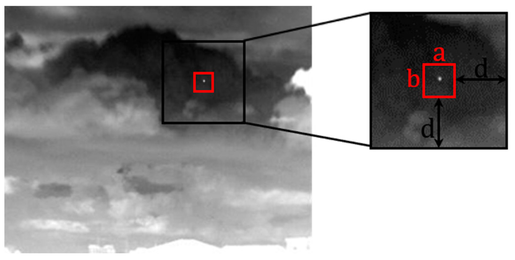
In addition, the SCRG and BSF can also be used to measure an algorithm’s ability to enhance the target and suppress the background, respectively. Both SCRG and BSF are calculated in the neighborhood of the target. As shown in Figure 6, if the target size is $a\times b$, then $(a+2d)\times (b+2d)$ denotes the size of the target neighborhood. In the experiments of this paper, we follow [32] to set $d=65$.

The SCRG represents the SCR of the detection result and the original image, which is expressed as:

$$\mathrm{S}\mathrm{C}\mathrm{R}\mathrm{G}=\frac{{\mathrm{S}\mathrm{C}\mathrm{R}}_{\mathrm{o}\mathrm{u}\mathrm{t}}}{{\mathrm{S}\mathrm{C}\mathrm{R}}_{\mathrm{i}\mathrm{n}}}$$

(46)

where SCR reflects the degree of discrimination between the target and the background clutter in the image, which can be calculated as:

$$\mathrm{S}\mathrm{C}\mathrm{R}=\frac{\left|{\overline{\mu }}_0-{\overline{\mu }}_1\right|}{{\mathsf{\sigma }}_1}$$

(47)

where ${\overline{\mu }}_0$ denotes the target’s average gray value, ${\overline{\mu }}_1$ denotes that of the target neighborhood, and ${\mathsf{\sigma }}_1$ denotes the gray standard deviation of the target neighborhood.

The BSF can evaluate the background suppression ability, which is defined as follows:

$$\mathrm{B}\mathrm{S}\mathrm{F}=\frac{{\mathsf{\sigma }}_{\mathrm{i}\mathrm{n}}}{{\mathsf{\sigma }}_{\mathrm{o}\mathrm{u}\mathrm{t}}}$$

(48)

where ${\mathsf{\sigma }}_{\mathrm{o}\mathrm{u}\mathrm{t}}$ and ${\mathsf{\sigma }}_{\mathrm{i}\mathrm{n}}$ represent the standard deviations of the target neighborhood in the detection result and the original image, respectively.

4.3. Parameter Analyses

The settings of different parameters in the model have a great impact on the detection performance. Therefore, this section aims to explore the appropriate parameters for the TTALP-TV method in sequences 1–6. According to [61], we set ${\lambda }_2=0.01$. Then, we detail the effects of $L$ and $H$ on the detection capability of our proposed method.

4.3.1. Adjacent Frames Number $L$

In the construction of the spatial–temporal tensor, the adjacent frame number $L$ determines the utilization of temporal domain information. In order to investigate the influence of different $L$ values on the detection performance of the TTALP-TV model, we adjust $L$ from 2 to 6 with a step of 1. Figure 7 shows the analysis results of various $L$ values using the 3D ROC. Increasing the $L$ values can incorporate more temporal information, which ensures the low-rankness of the spatial–temporal tensor. At the same time, over-large adjacent frame numbers will lead to redundant and repetitive information, resulting in high false alarms. Figure 7 shows that $L=3$ is the most suitable for the proposed model.

4.3.2. Tuning Parameter $H$

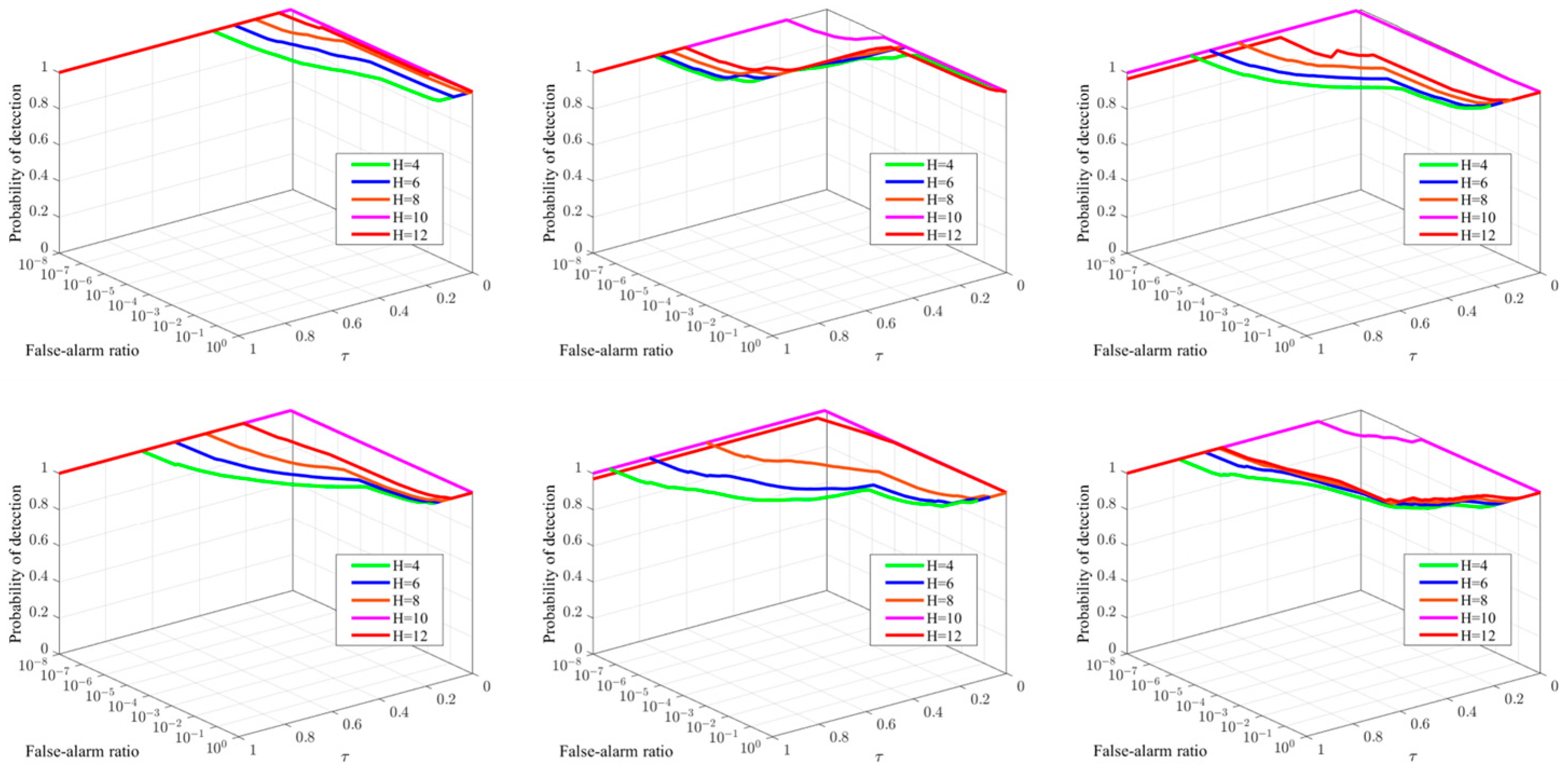
The compromising parameter ${\lambda }_1$ controls the balance between the sparse target and the low-rank background in the framework. Following [62], we set ${\lambda }_1=H∕\sqrt{max\left(n_1,n_2\right)\ast L}$, where $H$ is a crucial tuning parameter. We change $H$ from 4 to 12 with a step of 2. The 3D ROC analysis results of $H$ are shown in Figure 8. It can be seen from Figure 8 that when $H$ values increase, the false alarms decrease, which indicates that $H$ assists in the suppression of background residuals. Meanwhile, if $H$ is too large (e.g., $H=12$), some necessary information may be lost, resulting in the degradation of detection performance. Based on the 3D ROC analysis results shown in Figure 8, we set $H=10.$

4.4. Ablation Study

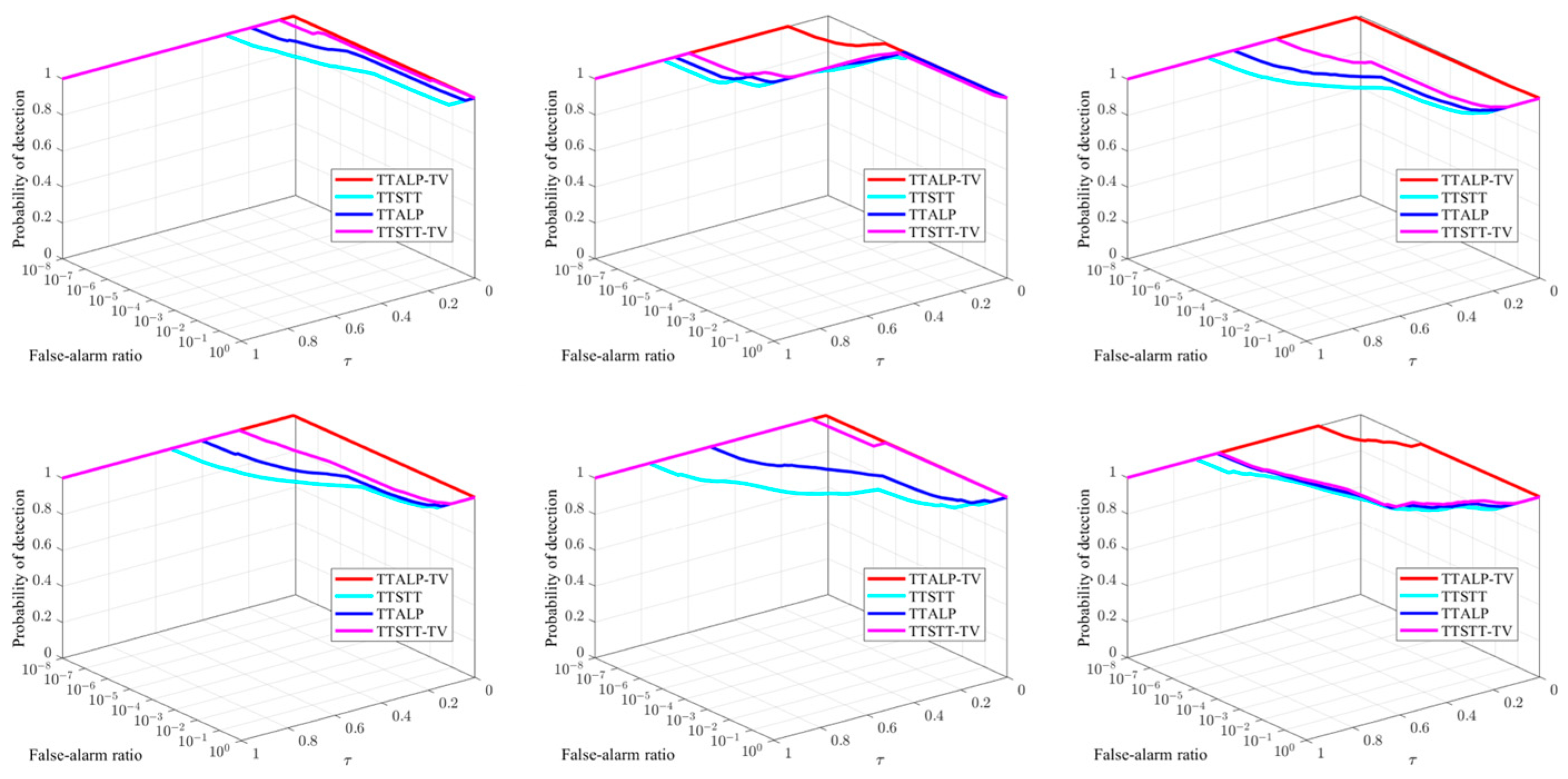
In order to validate the effectiveness of the self-adaptive local prior and STTV regularization in the proposed TTALP-TV method, we conducted an ablation study, as shown in Figure 9. The TTALP-TV framework consists of three parts: the tensor tree-based spatiotemporal tensor model, the self-adaptive local prior tensor, and STTV regularization. As illustrated in Figure 9, we compare the 3D ROC analysis results of four versions of the TTALP-TV method in sequences 1–6: (1) the tensor tree-based spatiotemporal tensor model (TTSTT), (2) incorporating self-adaptive local prior tensor into the tensor tree-based spatiotemporal tensor model (TTALP), (3) imposing STTV regularization constraint on the background component in the tensor tree-based spatiotemporal tensor model (TTSTT-TV), and (4) integrating the self-adaptive local prior tensor and STTV regularization into the tensor tree-based spatiotemporal tensor model (TTALP-TV). Figure 9 shows that leveraging the self-adaptive local prior does in fact improve target detection performance to a certain extent. Moreover, the STTV regularization constraint on the background helps better remove background clutter and noise while preserving image details. The results of the ablation experiments intuitively demonstrate the significance of any single module and provide guidance for further attempts to improve the optimization model.

4.5. Noise Robustness Validation of the Proposed TTALP-TV Method

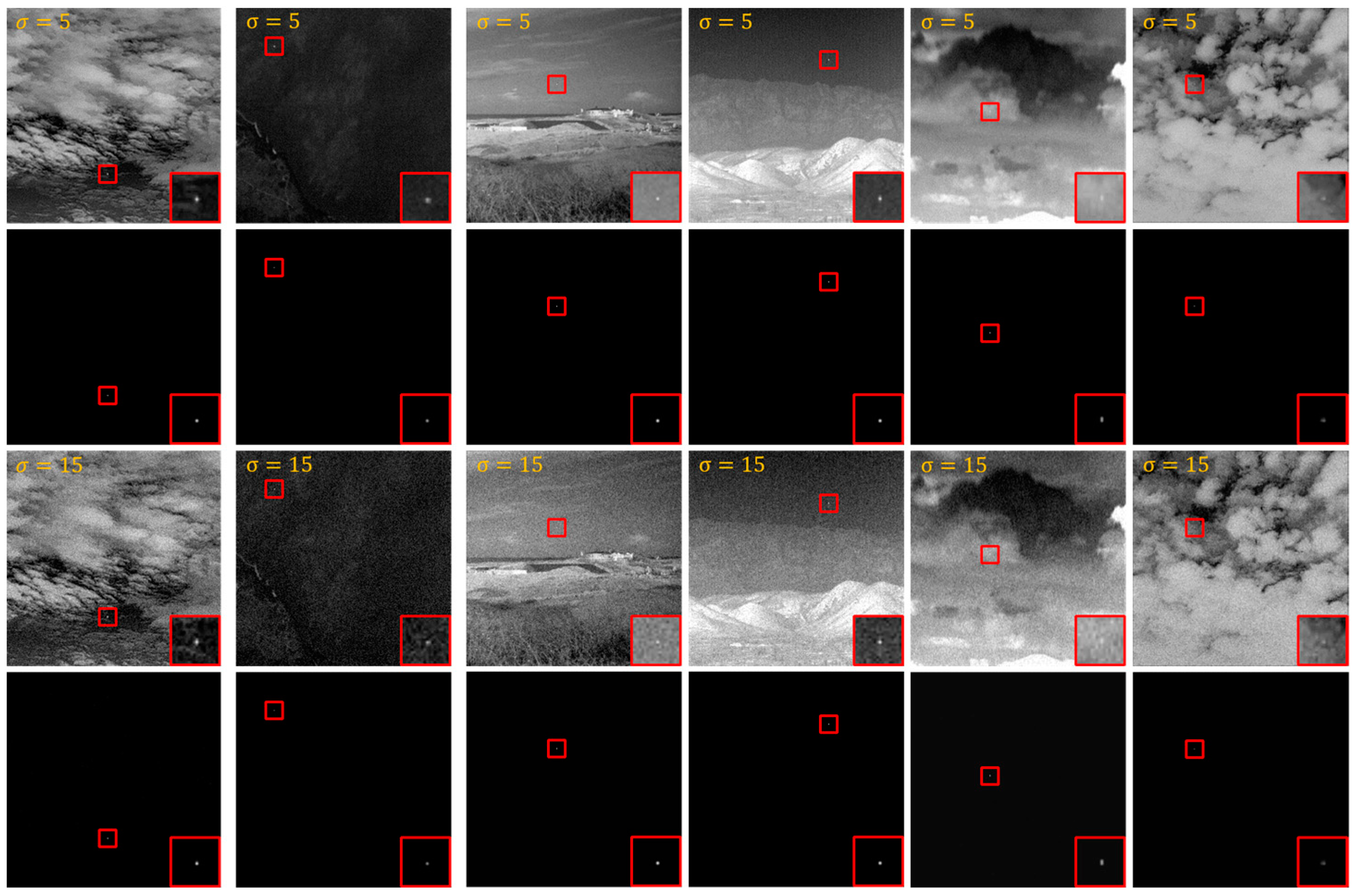
Due to the influence of the real-world environment on the sensor, infrared images usually contain noise. Therefore, it is essential to evaluate the robustness of the TTALP-TV model to noise. To evaluate the noise robustness of TTALP-TV under different noise intensities, Gaussian white noise of $\sigma =5$ and $\sigma =15$ was added to six scenes, respectively. The second and fourth rows of Figure 9 show the visual detection results of $\sigma =5$ and $\sigma =15$, respectively. Figure 10 shows that TTALP-TV can accurately detect targets and suppress noise of different intensities, demonstrating its robustness to noisy scenes.

4.6. Comparison with State-of-the-Art Methods

In order to assess the advantages of the TTALP-TV method, we compare it with eight representative baseline methods. These methods can be categorized into background consistency-based methods (Top-hat [7]), HVS-based methods (TLLCM [16]), LRSD-based single-frame detection methods (IPI [22], PSTNN [31], NTFRA [32], and ANLPT [33]) and LRSD-based sequential-frame detection methods (ASTTV-NTLA [63] and NFTDGSTV [42]).

Table 3. Detailed parameters of nine methods.

Method	Parameters
Top-hat	Shape: disk, structure size: $5\times 5$.
TLLCM	Different filtering window: $3\times 3$, $5\times 5$, $7\times 7$.
IPI	Patch size: $50\times 50$, step: 10, $\lambda =1∕\sqrt{min\left(m,n\right)}$, $\epsilon ={10}^{-7}$.
PSTNN	Patch size: $40\times 40$, step: 40, $\lambda =0.7∕\sqrt{min\left(n_1,n_2\right)\ast n_3}$, $\epsilon ={10}^{-7}$.
ASTTV-NTLA	$L=3$, $H=6$, ${\lambda }_{tv}=0.005$, ${\lambda }_s=\frac{H}{\sqrt{max\left(M,N\right)\ast L}}$, ${\lambda }_3=100$.
NTFRA	Patch size: $40\times 40$, step: 40, $\lambda =1∕\sqrt{min\left(n_1,n_2\right)\ast n_3}$, $\beta =0.05$, $\mu =200$.
ANLPT	Patch size: $50\times 50$, step: 50, region: 10, channel: 3, $\mu ={10}^{-3}$.
NFTDGSTV	$L=3$, $H=4$, ${\lambda }_1=0.01$, ${\lambda }_2=\frac{H}{\sqrt{max\left(M,N\right)\ast L}}$, ${\lambda }_s=0.001$.
Proposed	$L=3$, $H=10$, ${\lambda }_1=\frac{H}{\sqrt{max\left(n_1,n_2\right)\ast L}}$, ${\lambda }_2=0.01$.

lists the detailed parameter settings of these methods.

4.6.1. Visual Comparison

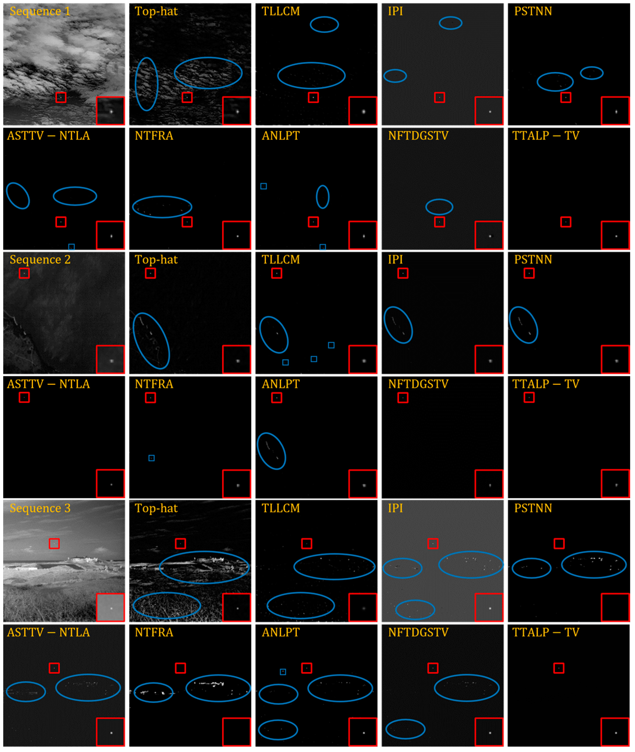
Figure 11 and Figure 12 show the detection results of eight compared methods and our method in six infrared sequences. From Figure 11 and Figure 12, we can see that Top-hat has a lot of clutter and noise residuals in its detection results. The main reason for this is that the structure size of the Top-hat is fixed, meaning it cannot adapt to the dynamics of complex scenes. In contrast, TLLCM suppresses clutter to a certain extent but still has background residuals in complex scenes. Compared with the background consistency and HVS methods, the matrix-based LRSD method IPI contains fewer background residuals, but its background is gray. As can be seen from Figure 11 and Figure 12, the PSTNN and ANLPT methods can achieve relatively better target detection performance (e.g., sequences 1, 4, and 6), but they are basically unable to completely suppress background.

At the same time, we can see that NTFRA can better preserve targets and suppress background interference but fails in complex scenes with highlighted line edges (e.g., sequences 3–4). These single-frame detection methods effectively utilize spatial information to separate the target from the background. However, using only inter-frame information results in low robustness to various complex scenes with dynamic changes and heavy clutter. Therefore, many researchers have combined spatial–temporal information to improve detection ability and remove background interference. It can be seen from Figure 11 and Figure 12 that ASTTV-NTLA and NFTDGSTV present exceptional target detection and background suppression abilities in scenes with little clutter interference (e.g., sequence 2). However, when faced with complex scenes with high-brightness clutter and heavy noise (e.g., sequences 3, 4, and 6), their detection performance will degrade significantly. In contrast, the proposed TTALP-TV method is not only able to accurately extract the target and preserve a relatively complete shape, but it can also mostly suppress strong edges and bright corner-point noise in complex scenes.

4.6.2. Quantitative Analysis

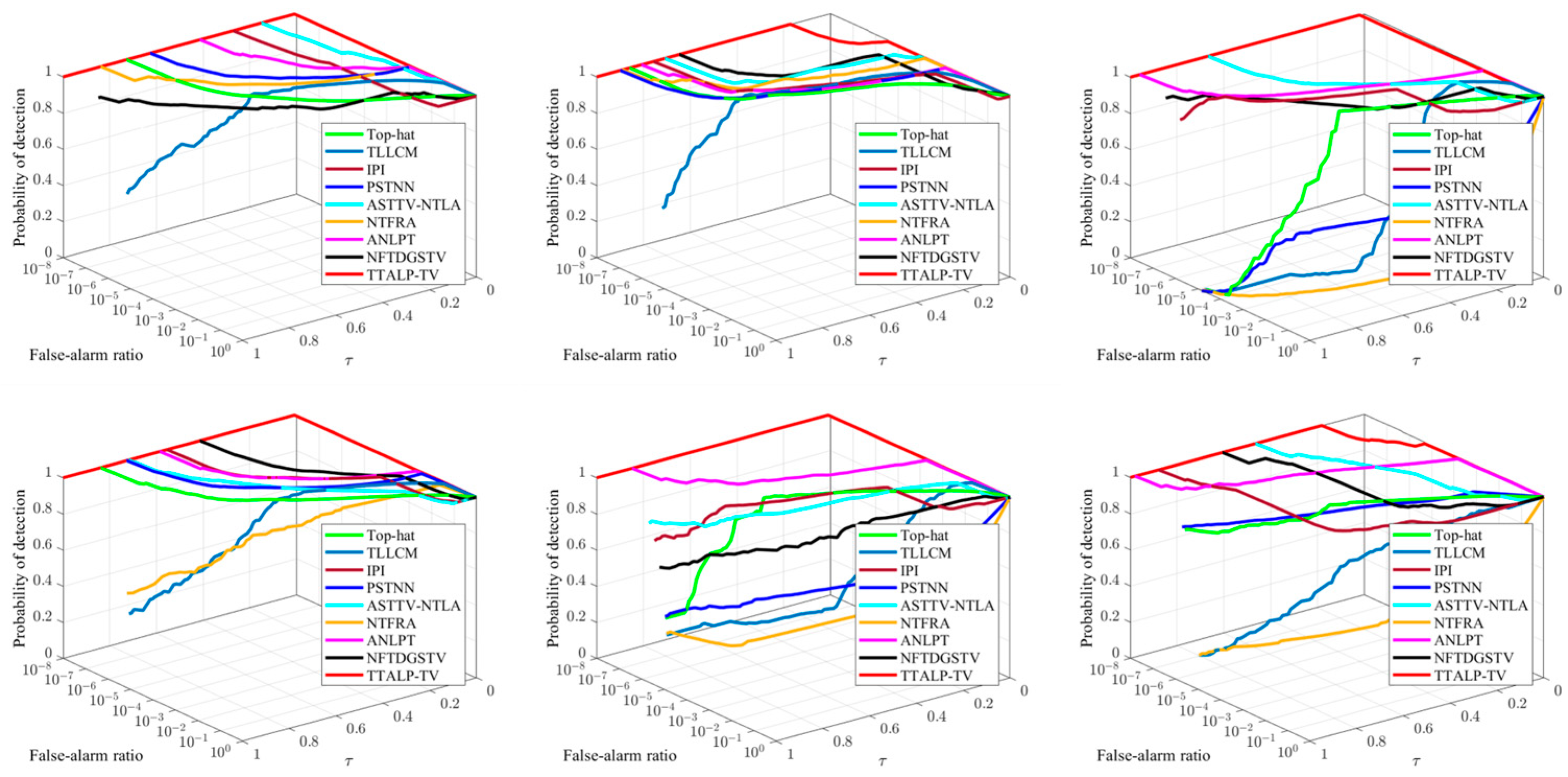
In addition to the qualitative analysis in Figure 11 and Figure 12, we adopt 3D ROC, ${\mathrm{A}\mathrm{U}\mathrm{C}}_{\mathrm{O}\mathrm{A}}$, ${\mathrm{A}\mathrm{U}\mathrm{C}}_{\mathrm{S}\mathrm{N}\mathrm{P}\mathrm{R}}$, SCRG, and BSF, a total of five evaluation metrics, to compare nine methods quantitatively. Figure 13 shows the 3D ROC curves of all comparison methods in complex and noisy scenes (e.g., sequences 1–6). In order to clearly depict the differences among the nine methods, the logarithmic scale is used for the false alarm rate axis. As shown in Figure 13, the proposed TTALP-TV method is closer to the top-right corner, indicating that it has superior detection performance. The single-frame detection method ANLPT also achieves good detection performance in sequence 5. Meanwhile, other sequential-frame detection methods, ASTTV-NTLA and NFTDGSTV, exhibit performance similar to our method in sequence 2 and sequence 6, but were not good enough in the rest of the sequences. To further assess which method has the best performance, we use ${\mathrm{A}\mathrm{U}\mathrm{C}}_{\mathrm{O}\mathrm{A}}$ and ${\mathrm{A}\mathrm{U}\mathrm{C}}_{\mathrm{S}\mathrm{N}\mathrm{P}\mathrm{R}}$ to evaluate target detection ability and background suppression ability, respectively. In each sequence, the highest value is highlighted in red, and the second highest value is marked in green.

Table 4. ${\mathrm{A}\mathrm{U}\mathrm{C}}_{\mathrm{O}\mathrm{A}}$ and ${\mathrm{A}\mathrm{U}\mathrm{C}}_{\mathrm{S}\mathrm{N}\mathrm{P}\mathrm{R}}$ of nine methods in sequences 1–3.

Method	Sequence 1		Sequence 2		Sequence 3
	${\mathbf{A}\mathbf{U}\mathbf{C}}_{\mathbf{O}\mathbf{A}}$	${\mathbf{A}\mathbf{U}\mathbf{C}}_{\mathbf{S}\mathbf{N}\mathbf{P}\mathbf{R}}$	${\mathbf{A}\mathbf{U}\mathbf{C}}_{\mathbf{O}\mathbf{A}}$	${\mathbf{A}\mathbf{U}\mathbf{C}}_{\mathbf{S}\mathbf{N}\mathbf{P}\mathbf{R}}$	${\mathbf{A}\mathbf{U}\mathbf{C}}_{\mathbf{O}\mathbf{A}}$	${\mathbf{A}\mathbf{U}\mathbf{C}}_{\mathbf{S}\mathbf{N}\mathbf{P}\mathbf{R}}$
Top-hat	1.9279	13.9053	1.9722	36.1500	1.6818	9.5483
TLLCM	1.8827	115.6874	1.9228	158.0823	1.3038	39.1759
IPI	1.8275	5.8048	1.9445	18.0709	1.7117	3.4998
PSTNN	1.9945	187.9084	1.9943	180.1801	0.8804	39.4834
ASTTV-NTLA	1.9943	182.1271	1.9947	197.3122	1.8817	8.4660
NTFRA	1.9944	186.0783	1.9947	195.7341	0.4936	0.6221
ANLPT	1.9946	193.5168	1.9943	181.1781	1.9942	178.3936
NFTDGSTV	1.8983	10.8409	1.9762	42.2723	1.9065	12.3141
Proposed	1.9948	198.0273	1.9948	198.0127	1.9944	183.0405

and

Table 5. ${\mathrm{A}\mathrm{U}\mathrm{C}}_{\mathrm{O}\mathrm{A}}$ and ${\mathrm{A}\mathrm{U}\mathrm{C}}_{\mathrm{S}\mathrm{N}\mathrm{P}\mathrm{R}}$ of nine methods in sequences 4–6.

Method	Sequence 4		Sequence 5		Sequence 6
	${\mathbf{A}\mathbf{U}\mathbf{C}}_{\mathbf{O}\mathbf{A}}$	${\mathbf{A}\mathbf{U}\mathbf{C}}_{\mathbf{S}\mathbf{N}\mathbf{P}\mathbf{R}}$	${\mathbf{A}\mathbf{U}\mathbf{C}}_{\mathbf{O}\mathbf{A}}$	${\mathbf{A}\mathbf{U}\mathbf{C}}_{\mathbf{S}\mathbf{N}\mathbf{P}\mathbf{R}}$	${\mathbf{A}\mathbf{U}\mathbf{C}}_{\mathbf{O}\mathbf{A}}$	${\mathbf{A}\mathbf{U}\mathbf{C}}_{\mathbf{S}\mathbf{N}\mathbf{P}\mathbf{R}}$
Top-hat	1.9456	18.4296	1.8556	31.0480	1.8923	14.3259
TLLCM	1.8404	98.9758	1.4616	74.5013	1.4474	77.1831
IPI	1.8934	9.3979	1.7779	4.8744	1.5130	2.0540
PSTNN	1.9936	161.9100	1.1649	81.6425	1.7827	162.4838
ASTTV-NTLA	1.8760	8.0798	1.9490	22.9404	1.9047	10.5164
NTFRA	1.8710	47.7343	1.0384	37.7261	0.8706	45.0366
ANLPT	1.9944	184.8268	1.9947	196.1699	1.9947	196.9744
NFTDGSTV	1.9435	17.7605	1.7477	5.9553	1.7946	4.8739
Proposed	1.9948	198.0272	1.9947	198.0339	1.9948	198.0076

show that our method achieves the highest ${\mathrm{A}\mathrm{U}\mathrm{C}}_{\mathrm{O}\mathrm{A}}$ and ${\mathrm{A}\mathrm{U}\mathrm{C}}_{\mathrm{S}\mathrm{N}\mathrm{P}\mathrm{R}}$ values.

In

Table 6. SCRG and BSF of nine methods in sequences 1–3.

Method	Sequence 1		Sequence 2		Sequence 3
	SCRG	BSF	SCRG	BSF	SCRG	BSF
Top-hat	17.87	1.46	1.48	1.17	0.86	0.89
TLLCM	99.67	4.40	2.85	1.97	5.17	4.08
IPI	131.12	12.07	2.49	2.12	7.57	4.79
PSTNN	114.29	7.98	2.59	1.98	1.15	3.24
ASTTV-NTLA	219.24	15.33	2.63	2.52	9.01	4.63
NTFRA	81.11	6.20	2.34	2.27	0.16	1.56
ANLPT	178.28	11.19	2.59	1.95	9.37	4.23
NFTDGSTV	174.78	14.05	2.78	2.78	13.47	6.65
Proposed	235.51	17.83	3.56	3.46	19.51	8.86

and

Table 7. SCRG and BSF of nine methods in sequences 4–6.

Method	Sequence 4		Sequence 5		Sequence 6
	SCRG	BSF	SCRG	BSF	SCRG	BSF
Top-hat	7.79	3.66	14.00	4.29	9.63	2.17
TLLCM	20.94	6.33	32.75	10.46	27.26	6.69
IPI	19.83	11.11	26.56	11.49	25.01	7.94
PSTNN	25.85	12.63	29.74	17.10	62.06	10.56
ASTTV-NTLA	18.18	10.45	36.50	15.77	71.84	14.40
NTFRA	20.50	10.64	23.89	17.50	13.06	9.49
ANLPT	22.97	10.82	41.95	16.01	77.48	14.15
NFTDGSTV	23.18	12.18	29.53	12.56	55.45	12.09
Proposed	27.39	13.88	40.79	17.83	96.11	18.30

, the SCRG and BSF of nine methods in six sequences are displayed, with the highest and second highest values of SCRG and BSF marked in red and green, respectively. The results show that the ANLPT model achieves the highest SCRG values in sequence 5. On the other hand, the SCRG and BSF values of our model surpass other methods for more complex scenes (e.g., sequences 1–4 and 6). In summary, the above quantitative analyses demonstrate the effectiveness of our algorithm in both target enhancement and background suppression, particularly in complex scenes.

4.6.3. Running Time

In addition to the above evaluation metrics, computational efficiency is also a crucial factor in infrared target detection algorithms.

Table 8. Running time(s) of the nine methods.

Method	Sequence 1	Sequence 2	Sequence 3	Sequence 4	Sequence 5	Sequence 6
Top-hat	0.0958	0.0989	0.1008	0.1013	0.1098	0.1011
TLLCM	1.1209	1.0979	1.1193	1.1235	0.8603	1.2962
IPI	5.1073	4.7903	5.1192	5.8094	3.9534	5.9438
PSTNN	0.3605	0.2402	0.3105	0.3168	0.2845	0.2813
ASTTV-NTLA	2.0889	2.1002	2.0552	2.1045	1.4487	2.2719
NTFRA	1.4493	1.3904	1.4145	1.4965	1.2829	1.6751
ANLPT	1.5682	1.5437	1.4939	1.5961	1.2954	1.5260
NFTDGSTV	1.9258	2.0223	1.9534	1.8297	1.8025	2.4437
Proposed	2.3115	2.2845	2.3740	2.3182	1.7406	2.5226

presents the average running time of all comparison methods on six sequences (per frame). It should be noted that the image size of sequences 1–4 is $256\times 256$, and the image size of sequences 5–6 is $256\times 205$ and $296\times 237$, respectively. In general, the larger image size results in the longer running time. Based on Table 8, we can find that Top-hat has the shortest time cost. This is because Top-hat adopts a simple model architecture. It is worth noting that tensor-based algorithms are significantly quicker than the matrix-based IPI algorithm. Among the tensor-based methods, the running time of sequential-frame detection methods (e.g., ASTTV-NTLA, NFTDGSTV) is longer than that of single-frame detection methods (e.g., PSTNN, NTFRA, ANLPT). This is mainly because sequential-frame detection methods require more time to process the temporal domain information. From Table 8, it can be seen that the proposed method has a longer running time than ASTTV-NTLA and NFTDGSTV. This is because computing the self-adaptive prior in TTALP-TV increases costs in terms of time. Based on the qualitative and quantitative results shown in Figure 11, Figure 12 and Figure 13 and Table 4, Table 5, Table 6 and Table 7, it can be concluded that our method has better detection performance than the compared methods. Therefore, the extra running time of our method is acceptable.

5. Conclusions

In this article, the TTALP-TV model is proposed for infrared small target detection in complex scenes. Based on the theorem that the tensor tree decomposition can exploit the data structure in a more balanced strategy, we introduce tensor tree rank to obtain more accurate background estimation. It reduces storage costs and retains spatial and temporal correlation through a hierarchical method. In addition, a novel local prior weight is proposed for adaptively assigning weights to targets, which helps to better distinguish targets from similar objects. Meanwhile, STTV is used as a joint regularization term to remove noise while preserving image details. Therefore, the separation of target and background is converted into an optimization problem. Finally, we provide an efficient ADMM-based framework for solving the proposed TTALP-TV model. Extensive experiments demonstrate that the proposed algorithm not only can accurately detect the target but also effectively suppresses background clutter and noise in various complex scenes. However, the real-time performance of our method still needs to be improved due to the prior weight calculation in the model. In the future, our work will focus on establishing more efficient mechanisms to further simplify the calculation and improve detection efficiency.

References

- Rawat, S.S.; Verma, S.K.; Kumar, Y. Review on recent development in infrared small target detection algorithms. Procedia Comput. Sci. 2020, 167, 2496–2505. [Google Scholar] [CrossRef]
- Xiao, S.; Peng, Z.; Li, F. Infrared Cirrus Detection Using Non-Convex Rank Surrogates for Spatial-Temporal Tensor. Remote Sens. 2023, 15, 2334. [Google Scholar] [CrossRef]
- Gao, J.; Wang, L.; Yu, J.; Pan, Z. Structure Tensor-Based Infrared Small Target Detection Method for a Double Linear Array Detector. Remote Sens. 2022, 14, 4785. [Google Scholar] [CrossRef]
- Pang, D.; Shan, T.; Ma, P.; Li, W.; Liu, S.; Tao, R. A Novel Spatiotemporal Saliency Method for Low-Altitude Slow Small Infrared Target Detection. IEEE Geosci. Remote Sens. Lett. 2022, 19, 7000705. [Google Scholar] [CrossRef]
- Du, J.; Lu, H.; Zhang, L.; Hu, M.; Chen, S.; Deng, Y.; Shen, X.; Zhang, Y. A Spatial-Temporal Feature-Based Detection Framework for Infrared Dim Small Target. IEEE Trans. Geosci. Remote Sens. 2022, 60, 3000412. [Google Scholar] [CrossRef]
- Eysa, R.; Hamdulla, A. Issues on Infrared Dim Small Target Detection and Tracking. In Proceedings of the 2019 International Conference on Smart Grid and Electrical Automation (ICSGEA), Xiangtan, China, 10–11 August 2019; pp. 452–456. [Google Scholar]
- Rivest, J.-F.; Fortin, R. Detection of dim targets in digital infrared imagery by morphological image processing. Opt. Eng. 1996, 35, 1886–1893. [Google Scholar] [CrossRef]
- Deshpande, S.D.; Er, M.H.; Venkateswarlu, R.; Chan, P. Max-mean and max-median filters for detection of small targets. In Proceedings of the Optics & Photonics, Denver, CO, USA, 4 October 1999. [Google Scholar]
- Yang, L.; Yang, J.; Yang, K. Adaptive detection for infrared small target under sea-sky complex background. Electron. Lett. 2004, 40, 1. [Google Scholar] [CrossRef]
- Hadhoud, M.M.; Thomas, D.W. The two-dimensional adaptive LMS (TDLMS) algorithm. IEEE Trans. Circuits Syst. 1988, 35, 485–494. [Google Scholar] [CrossRef]
- Widrow, B.; Glover, J.R.; McCool, J.M.; Kaunitz, J.; Williams, C.S.; Hearn, R.H.; Zeidler, J.R.; Dong, J.E.; Goodlin, R.C. Adaptive noise cancelling: Principles and applications. Proc. IEEE 1975, 63, 1692–1716. [Google Scholar] [CrossRef]
- Cao, M.; Sun, D. Infrared weak target detection based on improved morphological filtering. In Proceedings of the 2020 Chinese Control And Decision Conference (CCDC), Hefei, China, 22–24 August 2020; pp. 1808–1813. [Google Scholar]
- Chen, C.L.P.; Li, H.; Wei, Y.; Xia, T.; Tang, Y.Y. A Local Contrast Method for Small Infrared Target Detection. IEEE Trans. Geosci. Remote Sens. 2014, 52, 574–581. [Google Scholar] [CrossRef]
- Wei, Y.; You, X.; Li, H. Multiscale patch-based contrast measure for small infrared target detection. Pattern Recognit. 2016, 58, 216–226. [Google Scholar] [CrossRef]
- Shi, Y.; Wei, Y.; Yao, H.; Pan, D.; Xiao, G. High-Boost-Based Multiscale Local Contrast Measure for Infrared Small Target Detection. IEEE Geosci. Remote Sens. Lett. 2018, 15, 33–37. [Google Scholar] [CrossRef]
- Han, J.; Moradi, S.; Faramarzi, I.; Liu, C.; Zhang, H.; Zhao, Q. A Local Contrast Method for Infrared Small-Target Detection Utilizing a Tri-Layer Window. IEEE Geosci. Remote Sens. Lett. 2020, 17, 1822–1826. [Google Scholar] [CrossRef]
- Ma, Y.; Liu, Y.; Pan, Z.; Hu, Y. Method of Infrared Small Moving Target Detection Based on Coarse-to-Fine Structure in Complex Scenes. Remote Sens. 2023, 15, 1508. [Google Scholar] [CrossRef]
- Fan, Z.; Bi, D.; Xiong, L.; Ma, S.; He, L.; Ding, W. Dim infrared image enhancement based on convolutional neural network. Neurocomputing 2018, 272, 396–404. [Google Scholar] [CrossRef]
- Zhao, B.; Wang, C.; Fu, Q.; Han, Z. A Novel Pattern for Infrared Small Target Detection with Generative Adversarial Network. IEEE Trans. Geosci. Remote Sens. 2021, 59, 4481–4492. [Google Scholar] [CrossRef]
- Zhang, M.; Zhang, R.; Zhang, J.; Guo, J.; Li, Y.; Gao, X. Dim2Clear Network for Infrared Small Target Detection. IEEE Trans. Geosci. Remote Sens. 2023, 61, 5001714. [Google Scholar] [CrossRef]
- Ying, X.; Liu, L.; Wang, Y.; Li, R.; Chen, N.; Lin, Z.; Sheng, W.; Zhou, S. Mapping Degeneration Meets Label Evolution: Learning Infrared Small Target Detection with Single Point Supervision. In Proceedings of the IEEE/CVF Conference on Computer Vision and Pattern Recognition, Vancouver, BC, Canada, 17–24 June 2023; pp. 15528–15538. [Google Scholar]
- Gao, C.; Meng, D.; Yang, Y.; Wang, Y.; Zhou, X.; Hauptmann, A.G. Infrared patch-image model for small target detection in a single image. IEEE Trans. Image Process. 2013, 22, 4996–5009. [Google Scholar] [CrossRef]
- Xie, Y.; Gu, S.; Liu, Y.; Zuo, W.; Zhang, W.; Zhang, L. Weighted Schatten p-norm minimization for image denoising and background subtraction. IEEE Trans. Image Process. 2016, 25, 4842–4857. [Google Scholar] [CrossRef]
- Dai, Y.; Wu, Y.; Song, Y. Infrared small target and background separation via column-wise weighted robust principal component analysis. Infrared Phys. Technol. 2016, 77, 421–430. [Google Scholar] [CrossRef]
- Dai, Y.; Wu, Y.; Song, Y.; Guo, J. Non-negative infrared patch-image model: Robust target-background separation via partial sum minimization of singular values. Infrared Phys. Technol. 2017, 81, 182–194. [Google Scholar] [CrossRef]
- Wang, X.; Peng, Z.; Kong, D.; Zhang, P.; He, Y. Infrared dim target detection based on total variation regularization and principal component pursuit. Image Vis. Comput. 2017, 63, 1–9. [Google Scholar] [CrossRef]
- Zhang, L.; Peng, L.; Zhang, T.; Cao, S.; Peng, Z. Infrared small target detection via non-convex rank approximation minimization joint l2,1 norm. Remote Sens. 2018, 10, 1821. [Google Scholar] [CrossRef]
- Wang, X.; Peng, Z.; Kong, D.; He, Y. Infrared dim and small target detection based on stable multisubspace learning in heterogeneous scene. IEEE Trans. Geosci. Remote Sens. 2017, 55, 5481–5493. [Google Scholar] [CrossRef]
- Zhang, T.; Peng, Z.; Wu, H.; He, Y.; Li, C.; Yang, C. Infrared small target detection via self-regularized weighted sparse model. Neurocomputing 2021, 420, 124–148. [Google Scholar] [CrossRef]
- Dai, Y.; Wu, Y. Reweighted infrared patch-tensor model with both nonlocal and local priors for single-frame small target detection. IEEE J. Sel. Top. Appl. Earth Obs. Remote Sens. 2017, 10, 3752–3767. [Google Scholar] [CrossRef]
- Zhang, L.; Peng, Z. Infrared small target detection based on partial sum of the tensor nuclear norm. Remote Sens. 2019, 11, 382. [Google Scholar] [CrossRef]
- Kong, X.; Yang, C.; Cao, S.; Li, C.; Peng, Z. Infrared small target detection via nonconvex tensor fibered rank approximation. IEEE Trans. Geosci. Remote Sens. 2021, 60, 5000321. [Google Scholar] [CrossRef]
- Zhang, Z.; Ding, C.; Gao, Z.; Xie, C. ANLPT: Self-Adaptive and Non-Local Patch-Tensor Model for Infrared Small Target Detection. Remote Sens. 2023, 15, 1021. [Google Scholar] [CrossRef]
- Reed, I.S.; Gagliardi, R.M.; Stotts, L.B. Optical moving target detection with 3-D matched filtering. IEEE Trans. Aerosp. Electron. Syst. 1988, 24, 327–336. [Google Scholar] [CrossRef]
- Tonissen, S.M.; Evans, R.J. Peformance of dynamic programming techniques for track-before-detect. IEEE Trans. Aerosp. Electron. Syst. 1996, 32, 1440–1451. [Google Scholar] [CrossRef]
- Li, Y.; Zhang, Y.; Yu, J.-G.; Tan, Y.; Tian, J.; Ma, J. A novel spatio-temporal saliency approach for robust dim moving target detection from airborne infrared image sequences. Inf. Sci. 2016, 369, 548–563. [Google Scholar] [CrossRef]
- Zhao, F.; Wang, T.; Shao, S.; Zhang, E.; Lin, G. Infrared moving small-target detection via spatiotemporal consistency of trajectory points. IEEE Geosci. Remote Sens. Lett. 2019, 17, 122–126. [Google Scholar] [CrossRef]
- Sun, Y.; Yang, J.; Long, Y.; An, W. Infrared small target detection via spatial-temporal total variation regularization and weighted tensor nuclear norm. IEEE Access 2019, 7, 56667–56682. [Google Scholar] [CrossRef]
- Zhang, P.; Zhang, L.; Wang, X.; Shen, F.; Pu, T.; Fei, C. Edge and Corner Awareness-Based Spatial–Temporal Tensor Model for Infrared Small-Target Detection. IEEE Trans. Geosci. Remote Sens. 2021, 59, 10708–10724. [Google Scholar] [CrossRef]
- Hu, Y.; Ma, Y.; Pan, Z.; Liu, Y. Infrared Dim and Small Target Detection from Complex Scenes via Multi-Frame Spatial—Temporal Patch-Tensor Model. Remote Sens. 2022, 14, 2234. [Google Scholar] [CrossRef]
- Wang, G.; Tao, B.; Kong, X.; Peng, Z. Infrared Small Target Detection Using Nonoverlapping Patch Spatial–Temporal Tensor Factorization with Capped Nuclear Norm Regularization. IEEE Trans. Geosci. Remote Sens. 2022, 60, 5001417. [Google Scholar] [CrossRef]
- Liu, T.; Yang, J.; Li, B.; Wang, Y.; An, W. Infrared Small Target Detection via Nonconvex Tensor Tucker Decomposition with Factor Prior. IEEE Trans. Geosci. Remote Sens. 2023, 61, 5617317. [Google Scholar] [CrossRef]
- Wu, F.; Yu, H.; Liu, A.; Luo, J.; Peng, Z. Infrared Small Target Detection Using Spatiotemporal 4-D Tensor Train and Ring Unfolding. IEEE Trans. Geosci. Remote Sens. 2023, 61, 5002922. [Google Scholar] [CrossRef]
- Romera-Paredes, B.; Pontil, M. A New Convex Relaxation for Tensor Completion. In Proceedings of the Advances in Neural Information Processing Systems, Harrahs and Harveys, Lake Tahoe, NV, USA, 5–10 December 2013; pp. 2967–2975. [Google Scholar]
- Yang, J.-H.; Zhao, X.-L.; Ji, T.-Y.; Ma, T.-H.; Huang, T.-Z. Low-rank tensor train for tensor robust principal component analysis. Appl. Math. Comput. 2020, 367, 124783. [Google Scholar] [CrossRef]
- Zhao, Q.; Zhou, G.; Xie, S.; Zhang, L.; Cichocki, A. Tensor ring decomposition. arXiv 2016, arXiv:1606.05535. [Google Scholar]
- Hackbusch, W.; Kühn, S. A new scheme for the tensor representation. J. Fourier Anal. Appl. 2009, 15, 706–722. [Google Scholar] [CrossRef]
- Bigun, J.; Granlund, G.H.; Wiklund, J. Multidimensional orientation estimation with applications to texture analysis and optical flow. IEEE Trans. Pattern Anal. Mach. Intell. 1991, 13, 775–790. [Google Scholar] [CrossRef]
- Brown, M.; Szeliski, R.; Winder, S. Multi-image matching using multi-scale oriented patches. In Proceedings of the 2005 IEEE Computer Society Conference on Computer Vision and Pattern Recognition (CVPR’05), San Diego, CA, USA, 20–25 June 2005; Volume 511, pp. 510–517. [Google Scholar]
- Frangi, A.F.; Niessen, W.J.; Vincken, K.L.; Viergever, M.A. Multiscale vessel enhancement filtering. In Proceedings of the Medical Image Computing and Computer-Assisted Intervention—MICCAI’98, Cambridge, MA, USA, 11–13 October 1998; Wells, W.M., Colchester, A., Delp, S., Eds.; Springer: Berlin/Heidelberg, Germany, 1998; pp. 130–137. [Google Scholar]
- Candes, E.J.; Eldar, Y.C.; Strohmer, T.; Voroninski, V. Phase retrieval via matrix completion. SIAM Rev. 2015, 57, 225–251. [Google Scholar] [CrossRef]
- Rudin, L.I.; Osher, S.; Fatemi, E. Nonlinear total variation based noise removal algorithms. Phys. D Nonlinear Phenom. 1992, 60, 259–268. [Google Scholar] [CrossRef]
- Liu, Y.; Long, Z.; Zhu, C. Image Completion Using Low Tensor Tree Rank and Total Variation Minimization. IEEE Trans. Multimed. 2019, 21, 338–350. [Google Scholar] [CrossRef]
- Boyd, S.; Parikh, N.; Chu, E.; Peleato, B.; Eckstein, J. Distributed optimization and statistical learning via the alternating direction method of multipliers. Found. Trends® Mach. Learn. 2011, 3, 1–122. [Google Scholar]
- Lin, Z.; Chen, M.; Ma, Y. The augmented lagrange multiplier method for exact recovery of corrupted low-rank matrices. arXiv 2010, arXiv:1009.5055. [Google Scholar]
- Cai, J.-F.; Candès, E.J.; Shen, Z. A singular value thresholding algorithm for matrix completion. SIAM J. Optim. 2010, 20, 1956–1982. [Google Scholar] [CrossRef]
- Beck, A.; Teboulle, M. A fast iterative shrinkage-thresholding algorithm for linear inverse problems. SIAM J. Imaging Sci. 2009, 2, 183–202. [Google Scholar] [CrossRef]
- Hui, B.; Song, Z.; Fan, H.; Zhong, P.; Hu, W.; Zhang, X.; Lin, J.; Su, H.; Jin, W.; Zhang, Y.; et al. A Dataset for Infrared Image Dim-Small Aircraft Target Detection and Tracking under Ground/Air Background; China Scientific Data: Beijing, China, 2019. [Google Scholar] [CrossRef]
- Sun, X.; Guo, L.; Zhang, W.; Wang, Z.; Yu, Q. Small Aerial Target Detection for Airborne Infrared Detection Systems Using LightGBM and Trajectory Constraints. IEEE J. Sel. Top. Appl. Earth Obs. Remote Sens. 2021, 14, 9959–9973. [Google Scholar] [CrossRef]
- Chang, C.-I. An effective evaluation tool for hyperspectral target detection: 3D receiver operating characteristic curve analysis. IEEE Trans. Geosci. Remote Sens. 2020, 59, 5131–5153. [Google Scholar] [CrossRef]
- Sun, L.; Zhan, T.; Wu, Z.; Jeon, B. A Novel 3D Anisotropic Total Variation Regularized Low Rank Method for Hyperspectral Image Mixed Denoising. ISPRS Int. J. Geo-Inf. 2018, 7, 412. [Google Scholar] [CrossRef]
- Lu, C.; Feng, J.; Chen, Y.; Liu, W.; Lin, Z.; Yan, S. Tensor robust principal component analysis with a new tensor nuclear norm. IEEE Trans. Pattern Anal. Mach. Intell. 2019, 42, 925–938. [Google Scholar] [CrossRef]
- Liu, T.; Yang, J.; Li, B.; Xiao, C.; Sun, Y.; Wang, Y.; An, W. Nonconvex Tensor Low-Rank Approximation for Infrared Small Target Detection. IEEE Trans. Geosci. Remote Sens. 2022, 60, 5614718. [Google Scholar] [CrossRef]
Figure 1.
Flowchart of the proposed TTALP-TV model for infrared small target detection.
Figure 2.
The diagram of tensor tree decomposition.
Figure 3.
Singular value distribution curves of infrared spatial–temporal tensor along each mode.
Figure 4.
Comparison of different local structure priors. Row 1 shows original infrared images. Rows 2 to 6 depict different local prior maps, obtained by Equation (13), RIPT, PSTNN, MFSTPT, and the proposed method, respectively. Columns (a–d) display the prior weights extracted using different calculation methods for four infrared image sequences.
Figure 5.
Representative frames corresponding to the six infrared sequences used in the experiments.
Figure 6.
Diagram of the target neighborhood.
Figure 7.
Three-dimensional ROC curves corresponding to different parameters of in the six sequences.
Figure 8.
Figure 9.
Ablation results of the six sequences in 3D ROC curves.
Figure 10.
Detection results of TTALP-TV under different noise intensities.
Figure 11.
Detection results of nine methods in sequences 1–3. The red rectangles denote target areas, and the blue ellipses denote noise and background residuals.
Figure 12.
Detection results of nine methods in sequences 4–6. The red rectangles denote target areas, and the blue ellipses denote noise and background residuals.
Figure 13.
Three-dimensional ROC curves of nine methods in sequences 1–6.