

Altimeter Calibrations in the Preliminary Four Years’ Operation of Wanshan Calibration Site

 , ,
, ,
Abstract
:1. Introduction
2. Introduction and Altimeter Calibration Method of WSCS
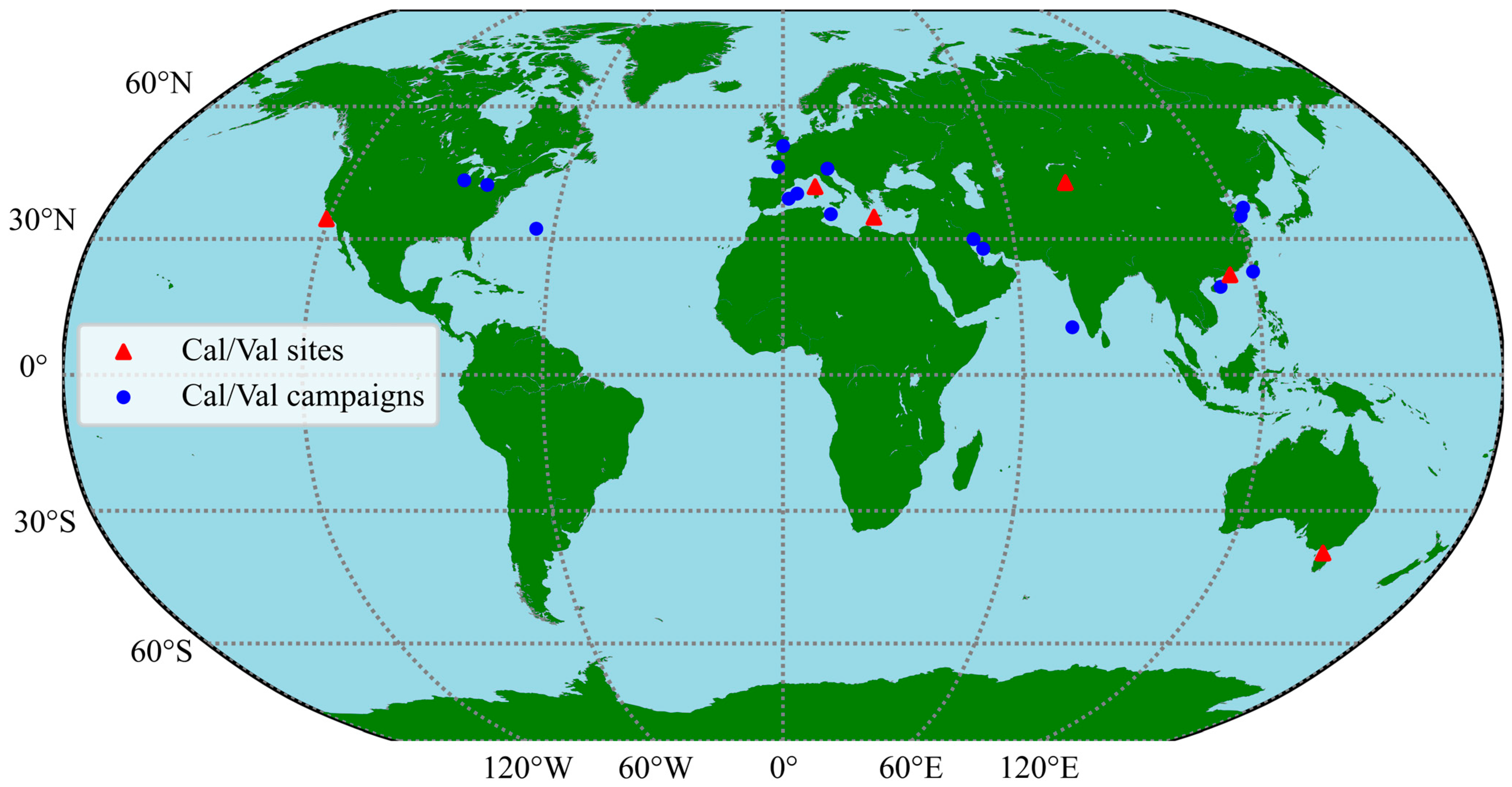
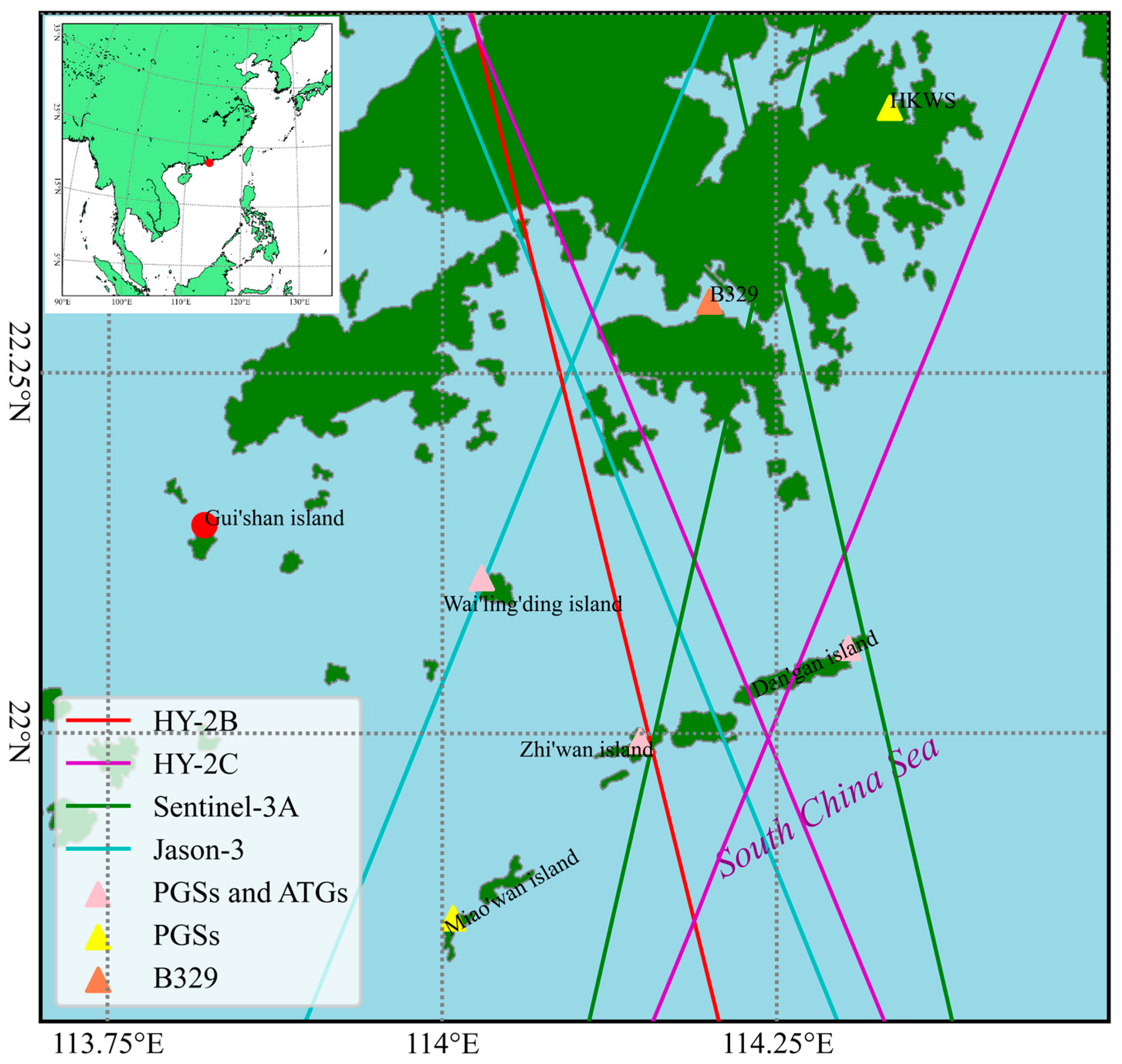
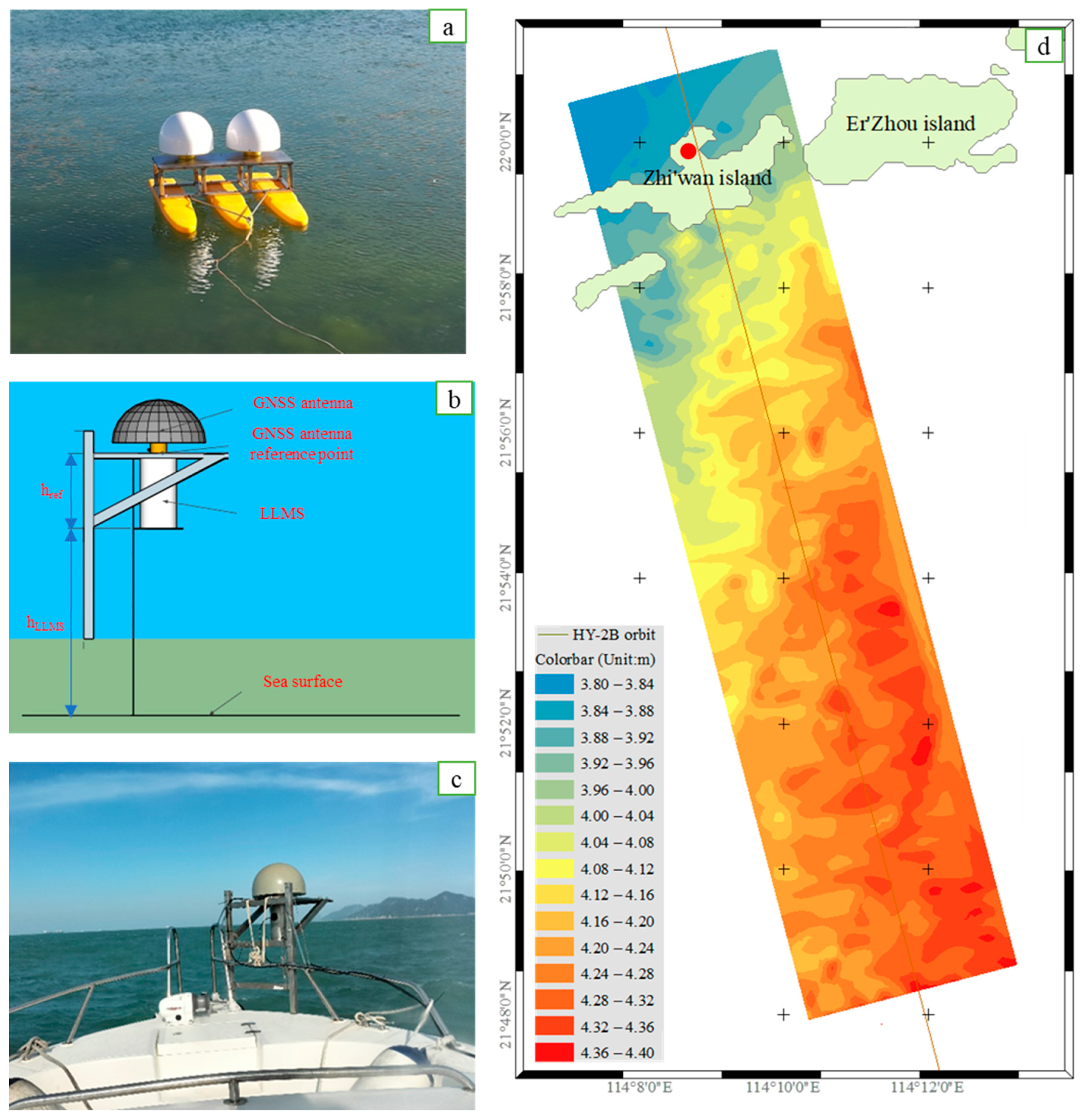
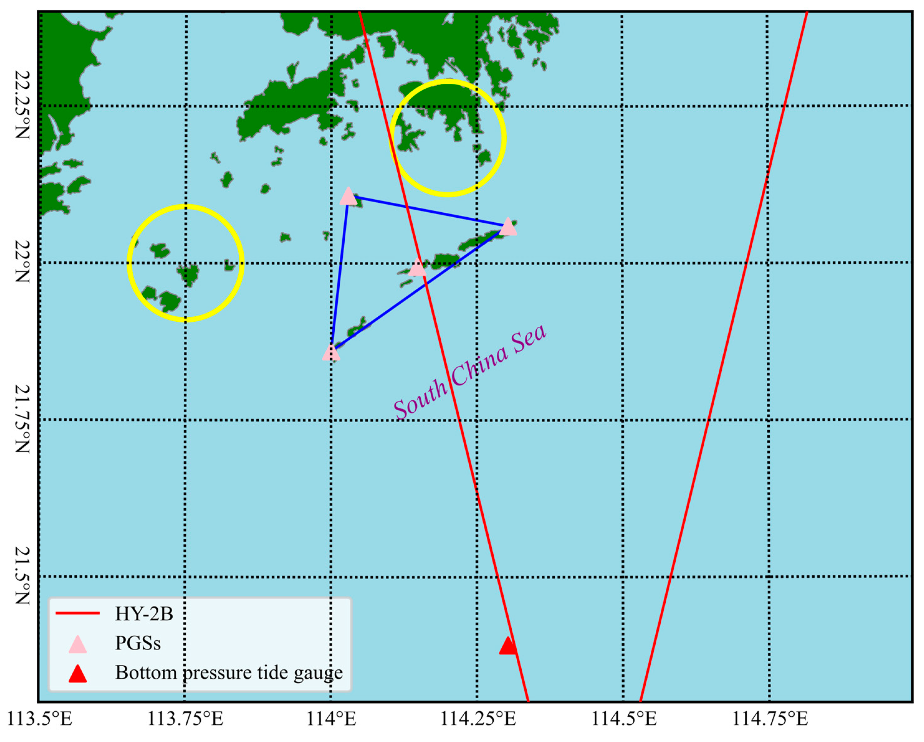
2.1. Introduction of WSCS
2.2. Altimeters and Calibration Methods
- where the H is the height of the altimeter above the ellipsoid;
- R is the range from the altimeters to the surface of the ocean;
- WZD/Dry is the wet/dry zenith delay caused by the wet and dry atmosphere, respectively;
- IC is the ionosphere correction;
- SSB is the sea state bias which was obtained using empirical models;
- SET is the solid Earth tide;
- LT is the loading tide height;
- PT is the pole tide.
- where the is the sea level of the in situ measurements at the time of altimeter overflight which was described in Section 3.2;
- DTidal is the tidal differences between the in situ measurements and the altimeter footprints which was described in Section 3.3.
- DMSS is the MSS differences between the ATGs and the altimeter footprints, which were described in Section 3.4.
3. Related Data and Correction Models in Cal/Val of Altimeters
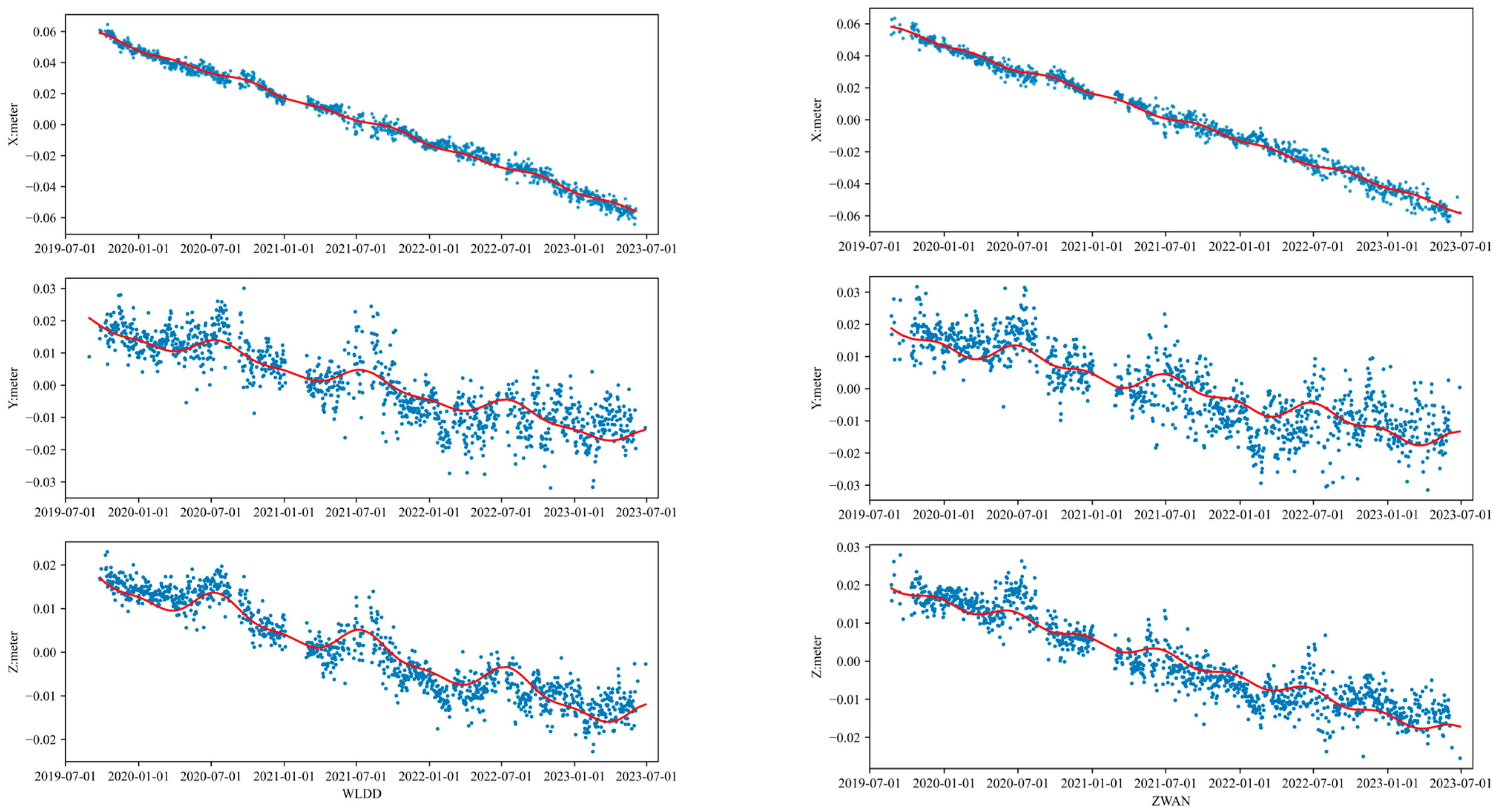
3.1. Datum of WSCS by the PGSs
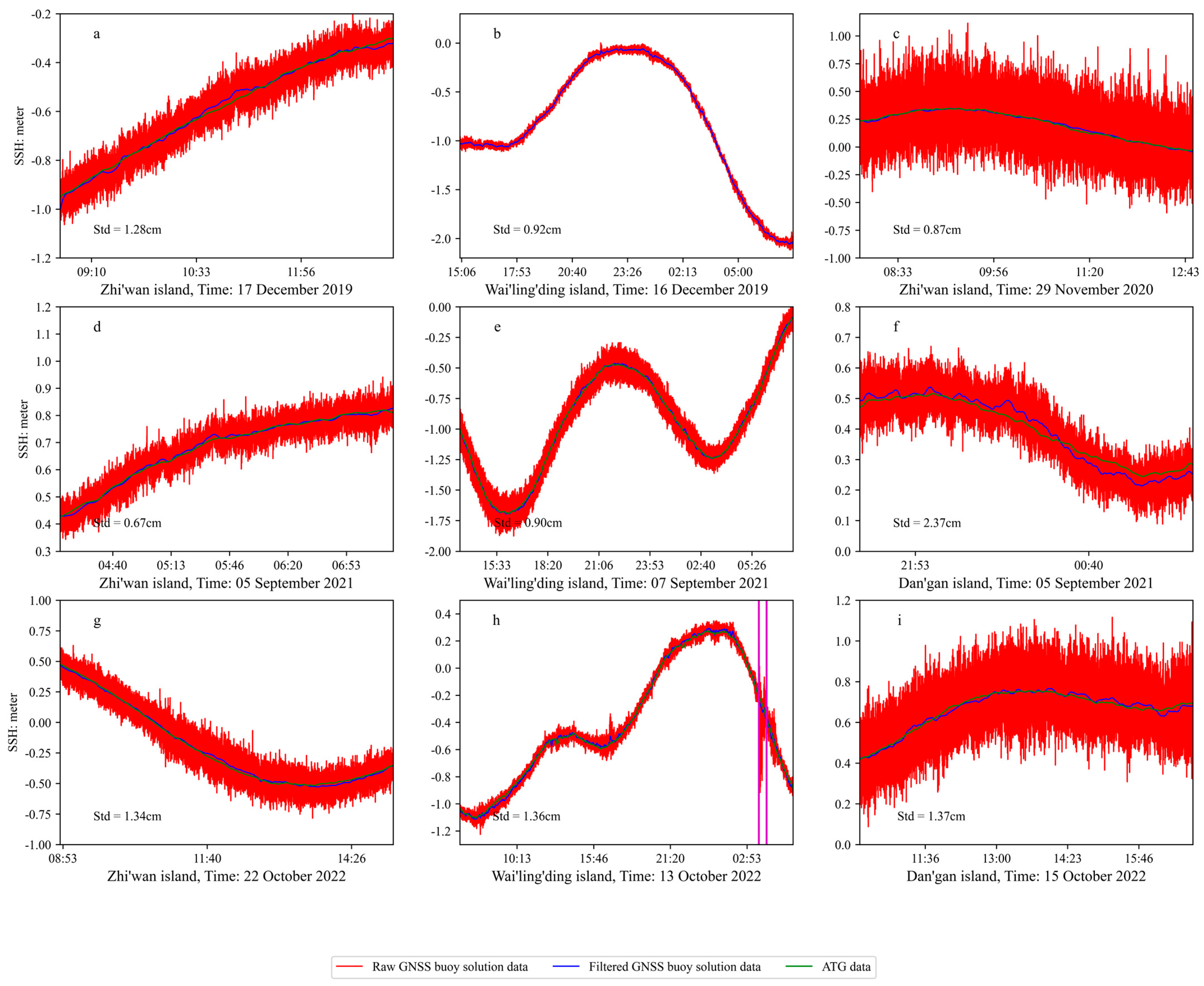
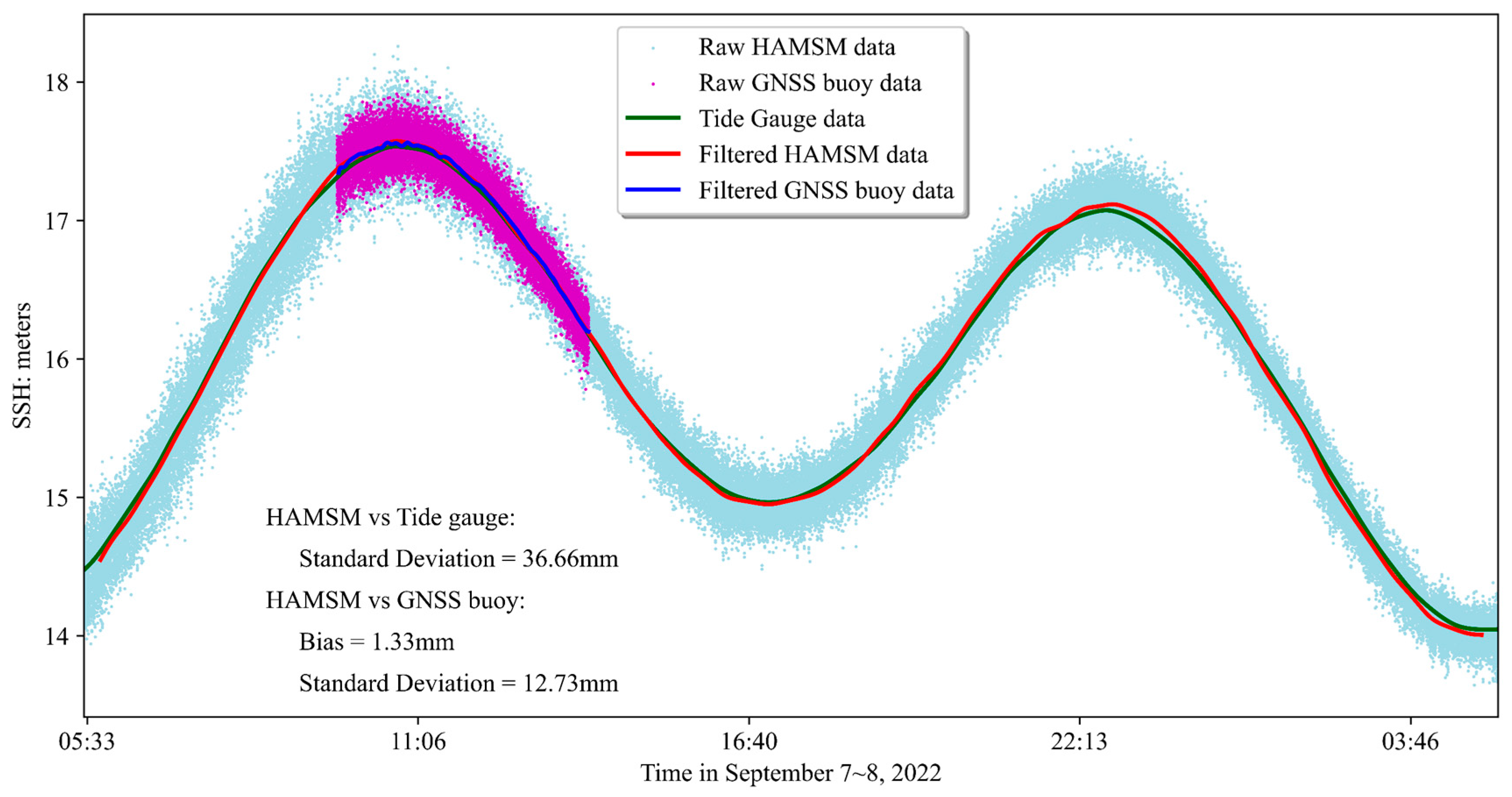
3.2. Datum of the In Situ SSH Measurements
- where, dh was the changes of the height caused by reference ellipsoid transformation;
- da = a0 − a, df = f0 − f were the corrections of the Semi-major Axis and flattening factor, respectively;
- a and a0 were the Semi-major Axis of WGS 84 and altimeter satellite, respectively;
- f and f0 were the Flattening Factor of the Earth of WGS 84 and altimeter satellite, respectively;
- was the latitude, and ;
- e was the first eccentricity of an ellipsoid.
3.3. Tidal Differences
- where the and represent the amplitude and Greenwich phase lag of a tide constituent given by the global tide models, respectively;
- The H and G are the amplitude and Greenwich phase lag derived from in situ tide gauges, respectively.
- where the is the vector difference at a specific location;
- N is the total number of tide gauges;
- is the RMS of constituent k.
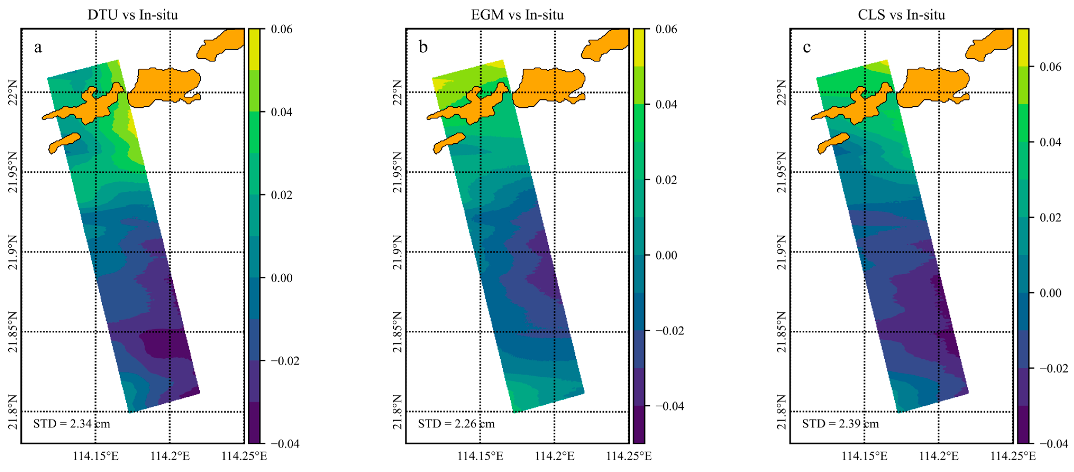
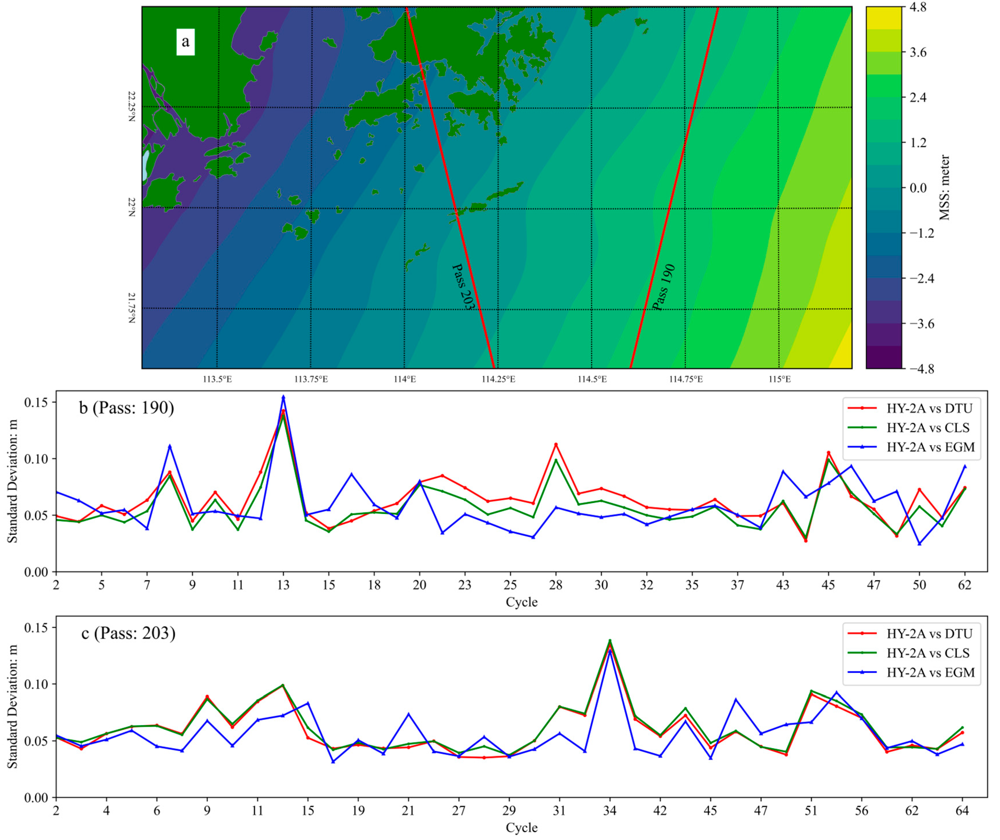
3.4. MSS
3.4.1. Campaigns of Sea Surface Measurements
- where the HGNSS ref is the height measured by the Chock ring antenna;
- href is the height from the Chock ring antenna reference point to the LLMS, which was measured within 1 mm;
- hLLMS is the height from the LLMS to the sea surface.
3.4.2. Mean Sea Surface Models
4. Calibration Results
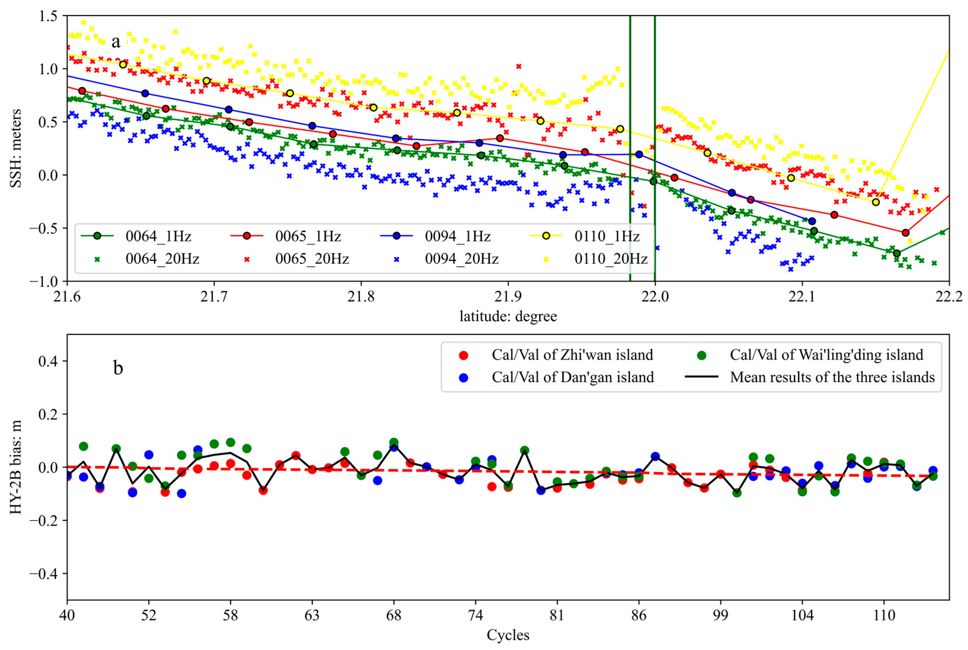
4.1. HY-2B
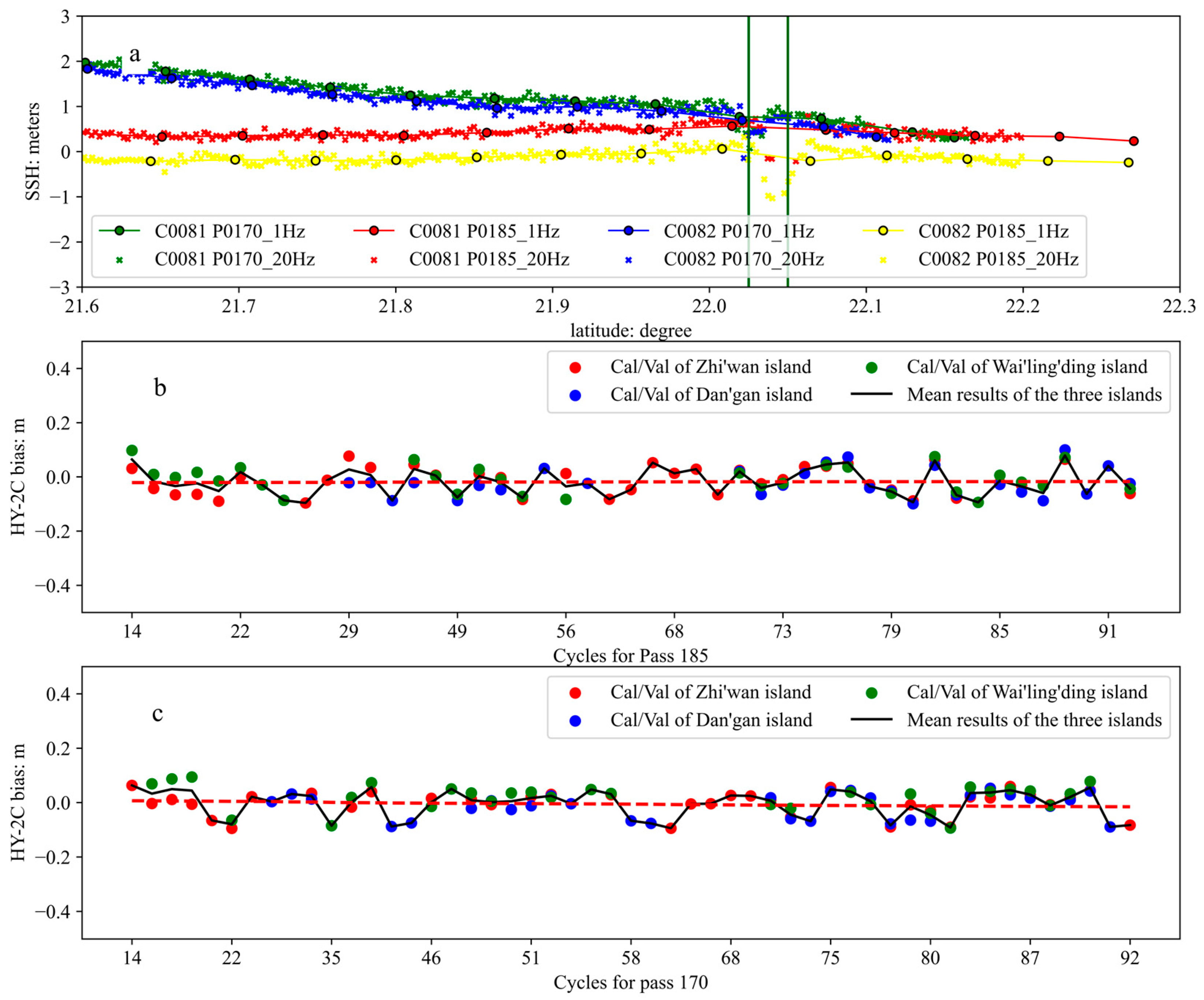
4.2. HY-2C
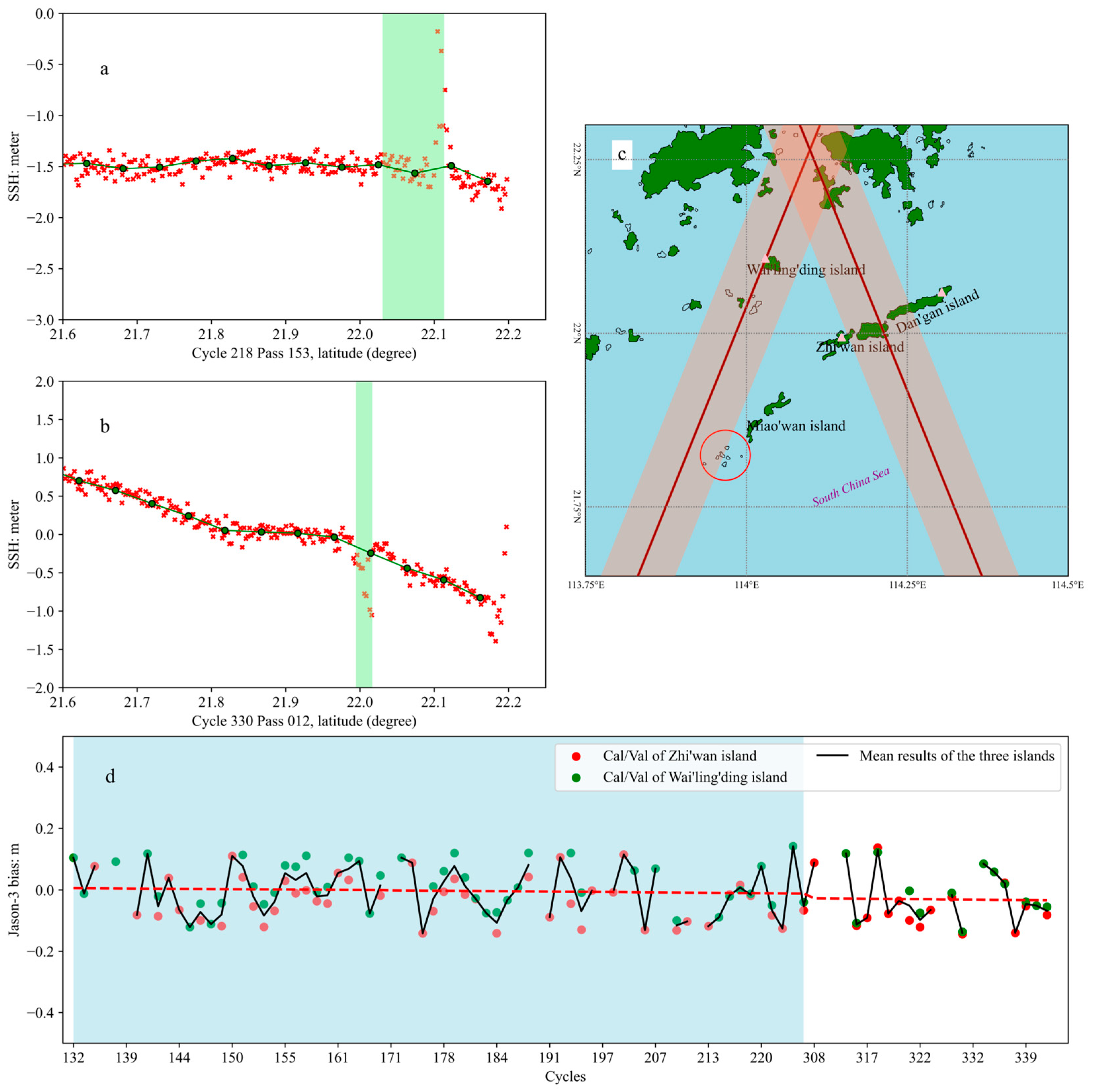
4.3. Jason-3
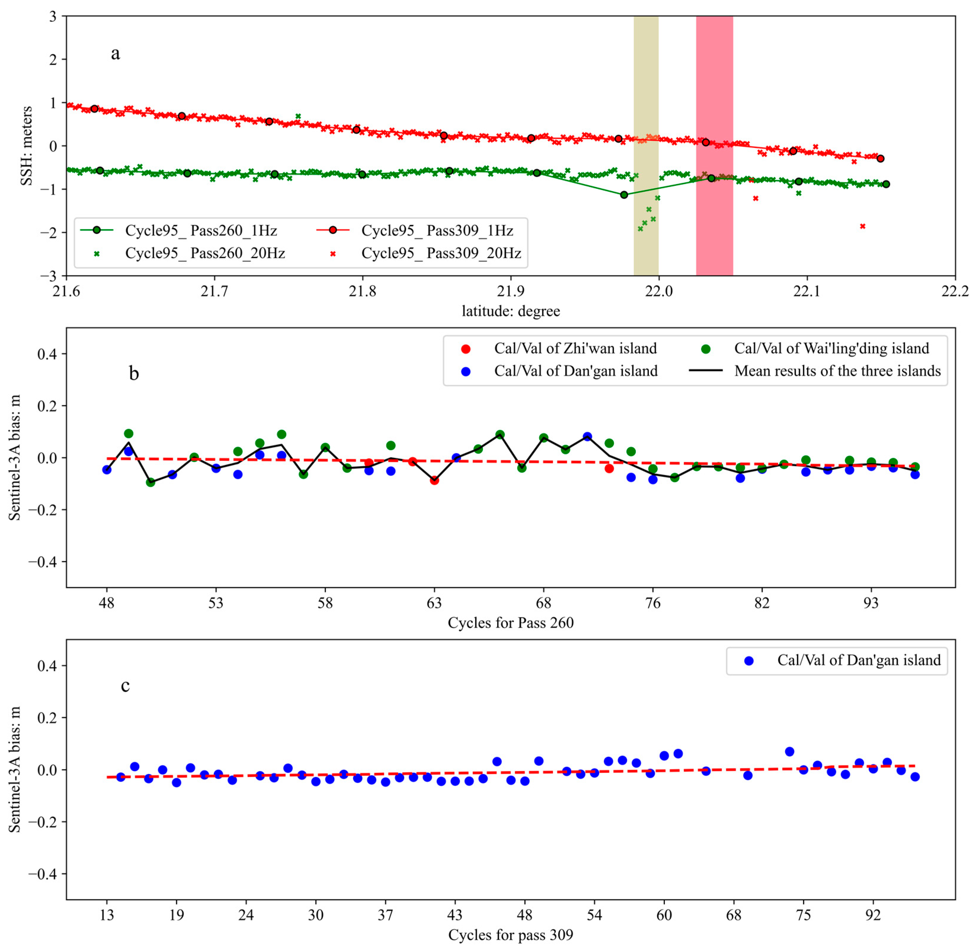
4.4. Sentinel-3A
5. Discussion
6. Conclusions
Author Contributions
Funding
Data Availability Statement
Acknowledgments
Conflicts of Interest
References
- International Altimetry Team. Altimetry for the future: Building on 25 years of progress. Adv. Space Res. 2021, 68, 319–363. [Google Scholar] [CrossRef]
- Eldardiry, H.; Hossain, F.; Strinivasan, M.; Tsontos, V. Success Stories of Satellite Radar Altimeter Applications. Bull. Am. Meteorol. Soc. 2022, 103, 33–53. [Google Scholar] [CrossRef]
- Mertikas, S.P.; Lin, M.; Piretzidis, D.; Kokolakis, C.; Donlon, C.; Ma, C.; Zhang, Y.; Jia, Y.; Mu, B.; Frantzis, X.; et al. Absolute Calibration of the Chinese HY-2B Altimetric Mission with Fiducial Reference Measurement Standards. Remote Sens. 2023, 15, 1393. [Google Scholar] [CrossRef]
- Ménard, Y.; Jeansou, E.; Vincent, P. Calibration of the TOPEX/POSEIDON altimeters at Lampedusa: Additional results at Harvest. J. Geophys. Res. Ocean. 1994, 99, 24487–24504. [Google Scholar] [CrossRef]
- Bonnefond, P.; Exertier, P.; Laurain, O.; Guinle, T.; Féménias, P. Corsica: A 20-Yr multi-mission absolute altimeter calibration site. Adv. Space Res. 2021, 68, 1171–1186. [Google Scholar] [CrossRef]
- Haines, B.; Desai, S.D.; Kubitschek, D.; Leben, R.R. A brief history of the Harvest experiment: 1989–2019. Adv. Space Res. 2021, 68, 1161–1170. [Google Scholar] [CrossRef]
- Mertikas, S.P.; Donlon, C.; Femenias, P.; Mavrocordatos, C.; Galanakis, D.; Guinle, T.; Boy, F.; Tripolitsiotis, A.; Frantzis, X.; Tziavos, I.N.; et al. Absolute Calibration of Sentinel-3A and Jason-3 Altimeters with Sea-Surface and Transponder Techniques in West Crete, Greece. In Fiducial Reference Measurements for Altimetry (Part of the “International Association of Geodesy Symposia Book Series”); Springer: Berlin/Heidelberg, Germany, 2019; Volume 150, pp. 41–47. [Google Scholar]
- Dettmering, D.; Schwatke, C.; Bosch, W. Global Calibration of SARAL/AltiKa Using Multi-Mission Sea Surface Height Crossovers. Mar. Geod. 2015, 38, 206–218. [Google Scholar] [CrossRef]
- Watson, C.; White, N.; Church, J.; Burgette, R.; Tregoning, P.; Coleman, R. Absolute calibration in bass strait, Australia: TOPEX, Jason-1 and OSTM/Jason-2. Mar. Geod. 2011, 34, 242–260. [Google Scholar] [CrossRef]
- Bonnefond, P.; Exertier, P.; Laurain, O.; Thibaut, P.; Mercier, F. GPS-based sea level measurements to help the characterization of land contamination in coastal areas. Adv. Space Res. 2013, 51, 1383–1399. [Google Scholar] [CrossRef]
- Cancet, M.; Bijac, S.; Chimot, J.; Bonnefond, P.; Jeansou, E.; Laurain, O.; Lyard, F.; Bronner, E.; Féménias, P. Regional in situ validation of satellite altimeters: Calibration and cross-calibration results at the Corsican sites. Adv. Space Res. 2013, 51, 1400–1417. [Google Scholar] [CrossRef]
- Dong, X.; Woodworth, P.; Moore, P.; Bingley, R. Absolute Calibration of the TOPEX/POSEIDON Altimeters using UK Tide Gauges, GPS, and Precise, Local Geoid-Differences. Mar. Geod. 2002, 25, 189–204. [Google Scholar] [CrossRef]
- Yuan, J.; Guo, J.; Liu, X.; Zhu, C.; Niu, Y.; Li, Z.; Ji, B.; Ouyang, Y. Mean sea surface model over China seas and its adjacent ocean established with the 19-year moving average method from multi-satellite altimeter data. Cont. Shelf Res. 2020, 192, 104009. [Google Scholar] [CrossRef]
- Jin, T.Y.; Li, J.C.; Jiang, W.P. The global mean sea surface model WHU2013. Geod. Geodyn. 2016, 7, 202–209. [Google Scholar] [CrossRef]
- Yang, L.; Xu, Y.; Lin, M.; Ma, C.; Mertikas, S.P.; Hu, W.; Wang, Z.; Mu, B.; Zhou, X. Monitoring the Performance of HY-2B and Jason-2/3 Sea Surface Height via the China Altimetry Calibration Cooperation Plan. IEEE Trans. Geosci. Remote Sens. 2022, 60, 1–13. [Google Scholar] [CrossRef]
- Zhai, W.; Zhu, J.; Lin, M.; Ma, C.; Chen, C.; Huang, X.; Zhang, Y.; Zhou, W.; Wang, H.; Yan, L. GNSS Data Processing and Validation of the Altimeter Zenith Wet Delay around the Wanshan Calibration Site. Remote Sens 2022, 14, 6235. [Google Scholar] [CrossRef]
- Zhai, W.; Zhu, J.; Chen, C.; Zhou, W.; Yan, L.; Zhang, Y.; Huang, X.; Guo, K. Obtaining accurate measurements of the sea surface height from a GPS buoy. Acta Oceanol. Sin. 2023, 42, 78–88. [Google Scholar] [CrossRef]
- Zhai, W.; Zhu, J.; Ma, C.; Fan, X.; Yan, L.; Wang, H.; Chen, C. Measurement of the sea surface using a GPS towing-body in Wanshan area. Acta Oceanol. Sin. 2020, 39, 123–132. [Google Scholar] [CrossRef]
- Herring, T.; King, R.; McClusky, S. Introduction to GAMIT/GLOBK (Release 10.7); Massachusetts Institute of Technology: Cambridge, MA, USA, 2018; Available online: http://geoweb.mit.edu/gg/Intro_GG.pdf (accessed on 22 June 2020).
- Bos, M.S.; Fernandes, R.M.S.; Williams, S.D.P.; Bastos, L. Fast error analysis of continuous GNSS observations with missing data. J. Geod. 2013, 87, 351–360. [Google Scholar] [CrossRef]
- Vaclavovic, P.; Dousa, J. G-Nut/Anubis: Open-Source Tool for Multi-GNSS Data Monitoring with a Multipath Detection for New Signals, Frequencies and Constellations. In IAG 150 Years. International Association of Geodesy Symposia; Rizos, C., Willis, P., Eds.; Springer: Cham, Switzerland, 2015; p. 143. [Google Scholar] [CrossRef]
- Herring, T.A. TRACK GPS Kinematic Positioning Program, Version 1.07; Massachusetts Institute of Technology: Cambridge, MA, USA, 2017; Available online: http://geoweb.mit.edu/gg/courses/201705_Bristol/pdf/31-TRACK_Intro.pdf (accessed on 30 July 2023).
- OSTM. Jason-3 Products Handbook. 2017; Issue: 1, Rev: 4. Available online: https://www.ospo.noaa.gov/Products/documents/hdbk_j3.pdf (accessed on 30 July 2023).
- Lyard, F.H.; Allain, D.J.; Cancet, M.; Carrère, L.; Picot, N. FES2014 global ocean tide atlas: Design and performance. Ocean Sci. 2021, 17, 615–649. [Google Scholar] [CrossRef]
- Taguchi, E.; Stammer, D.; Zahel, W. Inferring deep ocean tidal energy dissipation from the global high-resolution data-assimilative HAMTIDE model. J. Geophys. Res. Ocean. 2014, 119, 4573–4592. [Google Scholar] [CrossRef]
- Hart-Davis, M.G.; Piccioni, G.; Dettmering, D.; Schwatke, C.; Passaro, M.; Seitz, F. EOT20: A global ocean tide model from multi-mission satellite altimetry. Earth Syst. Sci. 2021, 13, 3869–3884. [Google Scholar] [CrossRef]
- Matsumoto, K.; Takanezawa, T.; Ooe, M. Ocean Tide Models Developed by Assimilating TOPEX/POSEIDON Altimeter Data into Hydrodynamical Model: A Global Model and a Regional Model around Japan. J. Oceanogr. 2000, 56, 567–581. [Google Scholar] [CrossRef]
- Ray, R.D.; Erofeeva, S.Y. Long-Period Tidal Variations in the Length of Day. J. Geophys. Res. Solid Earth 2014, 119, 1498–1509. [Google Scholar] [CrossRef]
- Pawlowicz, R.; Beardsley, B.; Lentz, S. Classical tidal harmonic analysis including error estimates in MATLAB using T_TIDE. Comput. Geosci. 2002, 28, 929–937. [Google Scholar] [CrossRef]
- King, M.A.; Padman, L. Accuracy assessment of ocean tide models around Antarctica. Geophys. Res. Lett. 2005, 32. [Google Scholar] [CrossRef]
- Lei, J.; Li, F.; Zhang, S.; Ke, H.; Zhang, Q.; Li, W. Accuracy Assessment of Recent Global Ocean Tide Models Around Antarctica. Int. Arch. Photogramm. Remote Sens. Spat. Inf. Sci. 2017, 42, 1521–1528. [Google Scholar] [CrossRef]
- Sun, W.; Zhou, X.; Zhou, D.; Sun, Y. Advances and accuracy assessment of ocean tide models in the Antarctic Ocean. Front. Earth Sci. 2022, 10, 757821. [Google Scholar] [CrossRef]
- Bonnefond, P.; Exertier, P.; Laurain, O.; Ménard, Y.; Orsoni, A.; Jeansou, E.; Haines, B.J.; Kubitschek, D.G.; Born, G. Leveling the Sea Surface Using a GPS-Catamaran. Mar. Geod. 2003, 26, 319–334. [Google Scholar] [CrossRef]
- Andersen, O.B.; Rose, S.K.; Abulaitijiang, A.; Zhang, S.; Fleury, S. The DTU21 global mean sea surface and first evaluation. Earth Syst. Sci. Data 2023, 15, 4065–4075. [Google Scholar] [CrossRef]
- Pavlis, N.K.; Holmes, S.A.; Kenyon, S.C.; Factor, J.K. The development and evaluation of the Earth Gravitational Model 2008 (EGM2008). J. Geophys. Res. Solid Earth 2012, 117, B04406. [Google Scholar] [CrossRef]
- Mulet, S.; Rio, M.H.; Etienne, H.; Artana, C.; Cancet, M.; Dibarboure, G.; Feng, H.; Husson, R.; Picot, N.; Provost, C.; et al. The new CNES-CLS18 global mean dynamic topography. Ocean. Sci. 2021, 17, 789–808. [Google Scholar] [CrossRef]
- Pujol, M.; Schaeffer, P.; Faugère, Y.; Raynal, M.; Dibarboure, G.; Picot, N. Gauging the Improvement of Recent Mean Sea Surface Models: A New Approach for Identifying and Quantifying Their Errors. J. Geophys. Res. Ocean. 2018, 123, 5889–5911. [Google Scholar] [CrossRef]
- Andersen, O.B.; Knudsen, P. DNSC08 mean sea surface and mean dynamic topography models. J. Geophys. Res. Ocean. 2009, 114, 327–432. [Google Scholar] [CrossRef]
- Jiang, X.; Jia, Y.; Zhang, Y. Measurement analyses and evaluations of sea-level heights using the HY-2A satellite’s radar altimeter. Acta Oceanol. Sin. 2019, 38, 134–139. [Google Scholar] [CrossRef]
- Lin, M.S.; Wang, X.H.; Peng, H.L.; Zhao, Q.L.; Li, M. Precise orbit determination technology based on dual-frequency GPS solution for HY-2 satellite. Eng. Sci. 2014, 16, 97–101. [Google Scholar]


| PGS | N Slope | E Slope | U Slope | Noise Model | Solutions |
|---|---|---|---|---|---|
| ZWAN | −10.52 ± 0.35 | 30.74 ± 0.24 | −2.05 ± 0.91 | GGM | This research |
| −10.52 ± 0.38 | 30.74 ± 0.24 | −2.33 ± 0.80 | GGM + WN | ||
| WLDD | −10.00 ± 0.29 | 31.25 ± 0.26 | −1.73 ± 0.55 | GGM | |
| −10.01 ± 0.34 | 31.25 ± 0.27 | −1.76 ± 0.59 | GGM + WN | ||
| HKWS | −10.80 ± 0.31 | 30.95 ± 0.21 | −1.43 ± 0.68 | GGM | |
| −10.83 ± 0.29 | 30.95 ± 0.22 | −1.59 ± 0.60 | GGM + WN | ||
| −11.54 ± 0.18 | 32.57 ± 0.16 | 0.73 ± 0.52 | -- | SOPAC | |
| −11.40 ± 0.09 | 32.89 ± 0.14 | 0.32 ± 0.30 | -- | COMB | |
| −11.40 ± 0.10 | 32.94 ± 0.15 | 0.07 ± 0.30 | -- | JPL |
| Tide Model | Facility | Resolution (Degree) | Number of Tidal Constituents |
|---|---|---|---|
| FES2014 | Archiving, Validation, and Interpretation of Satellite Oceanographic (AVISO) | 1/16 | 34 |
| HAMTIDE12 | The Deutsches Geodätisches Forschungsinstitut, Technical University of Munich (DGFI-TUM) | 1/8 | 17 |
| DTU16 | Technical University of Denmark (DTU) | 1/16 | 10 |
| NAO99Jb | National Astronomical Observatory (NAO) | 1/12 | 16 |
| GOT4.10 | National Aeronautics and Space Administration (NASA) | 1/8 | 16 |
| EOT20 | DGFI-TUM | 1/8 | 17 |
| K1 | K2 | M2 | N2 | S2 | O1 | P1 | Q1 | RSS | RSS* | |
|---|---|---|---|---|---|---|---|---|---|---|
| DTU 16 | 2.60 | 1.46 | 9.03 | 2.52 | 2.10 | 5.88 | 0.78 | 1.64 | 4.17 | 4.20 |
| NAOOjb | 2.94 | 1.02 | 9.51 | 2.63 | 2.07 | 5.63 | 1.04 | 1.61 | 4.28 | 4.38 |
| GOT4.10 | 2.80 | 0.70 | 8.54 | 2.77 | 2.43 | 5.72 | 0.81 | 1.61 | 4.04 | 3.83 |
| HAMTIDE12 | 2.63 | 0.62 | 8.60 | 2.59 | 1.97 | 5.53 | 0.78 | 1.58 | 3.96 | 3.95 |
| EOT20 | 11.18 | 0.75 | 9.32 | 2.61 | 2.37 | 5.57 | 2.07 | 1.49 | 5.73 | 4.96 |
| FES2014 | 1.98 | 0.96 | 9.21 | 2.58 | 2.07 | 5.88 | 0.96 | 1.67 | 4.17 | 4.31 |
Disclaimer/Publisher’s Note: The statements, opinions and data contained in all publications are solely those of the individual author(s) and contributor(s) and not of MDPI and/or the editor(s). MDPI and/or the editor(s) disclaim responsibility for any injury to people or property resulting from any ideas, methods, instructions or products referred to in the content. |
© 2024 by the authors. Licensee MDPI, Basel, Switzerland. This article is an open access article distributed under the terms and conditions of the Creative Commons Attribution (CC BY) license (https://creativecommons.org/licenses/by/4.0/).
Share and Cite
Zhai, W.; Zhu, J.; Peng, H.; Chen, C.; Yan, L.; Wang, H.; Huang, X.; Zhou, W.; Guo, H.; Zhang, Y. Altimeter Calibrations in the Preliminary Four Years’ Operation of Wanshan Calibration Site. Remote Sens. 2024, 16, 1087. https://doi.org/10.3390/rs16061087
Zhai W, Zhu J, Peng H, Chen C, Yan L, Wang H, Huang X, Zhou W, Guo H, Zhang Y. Altimeter Calibrations in the Preliminary Four Years’ Operation of Wanshan Calibration Site. Remote Sensing. 2024; 16(6):1087. https://doi.org/10.3390/rs16061087
Chicago/Turabian StyleZhai, Wanlin, Jianhua Zhu, Hailong Peng, Chuntao Chen, Longhao Yan, He Wang, Xiaoqi Huang, Wu Zhou, Hai Guo, and Yufei Zhang. 2024. "Altimeter Calibrations in the Preliminary Four Years’ Operation of Wanshan Calibration Site" Remote Sensing 16, no. 6: 1087. https://doi.org/10.3390/rs16061087