Article

Investigating a Possible Correlation between NOAA-Satellite-Detected Electron Precipitations and South Pacific Tectonic Events

by
Cristiano Fidani
1,2,*,
Serena D’Arcangelo
1,3,
Angelo De Santis
1,
Loredana Perrone
1 and
Maurizio Soldani
1
1
Istituto Nazionale di Geofisica e Vulcanologia (INGV), 00143 Rome, Italy
2
Central Italy Electromagnetic Network (CIEN), 63100 Fermo, Italy
3
Department of Physics of the Earth and Astrophysics, Faculty of Physics, Universidad Complutense de Madrid (UCM), 28040 Madrid, Spain
*
Author to whom correspondence should be addressed.
Remote Sens. 2024, 16(6), 1059; https://doi.org/10.3390/rs16061059
Submission received: 6 February 2024 / Revised: 11 March 2024 / Accepted: 12 March 2024 / Published: 16 March 2024

Abstract

:
On 4 March 2021, a devastating M8.1 earthquake struck the Kermadec Islands of New Zealand. Given the tremendous energy released during the event, we sought to investigate the event’s potential impact on the ionosphere and the inner Van Allen Belt using data from the high-energy electron detectors on board the NOAA-18 satellite. The survey was also extended to the strongest shallow M6.5+ earthquakes occurring between 150° and 190° in longitude, and between −5° and −35° in latitude over the previous ten years. In nearly all cases, evident electron fluxes entering the loss cone were observed. To explore the possibility of a connection between ionospheric signals and tectonic events in this intensely active region, we analyzed electron losses from the inner Van Allen Belt, taking into account latitude, longitude, day/night times, and proximity to the South Atlantic Anomaly. Compared to previous studies, here only the most significant loss phenomena persistent in the ionosphere were considered. Particular interest was reserved for the intense electron loss events that had a duration spanning from a few to several minutes and occurred several hours before and after strong seismic events. Thereafter, time series of electron counting rates and strong Southern Pacific earthquakes were transformed into binary series, and the series multiplication was investigated. The results suggest four peaks of association, including a first couple between electron perturbations detected for ascending semi-orbits and seismic events and a second one between electron perturbations detected in the southern ionosphere and seismic events. They both anticipated the occurrence of earthquakes, occurring around 4 h before them. Other couples were observed between electron perturbations detected for descending semi-orbits and seismic events and between electron perturbations detected in the northern ionosphere and seismic events. They both occurred around 3 h after the occurrence of earthquakes. The case of perturbations anticipating seismic events has the intriguing properties of sustaining the hypothesis that a physical interaction occurred around 6 h before seismic events as in the West Pacific case. A physical model of electrons detected far several thousands of km from the earthquake epicenters was also presented. However, a simulation of random seismic events suggested that the null hypothesis cannot be fully rejected for these associations, prompting many more analyses and case studies.

1. Introduction

Explorations of the ionospheric radiation environment highlighted the role of particle detectors [1] on board Low Earth Orbit (LEO) satellites in characterizing electron bursts. After the discovery of the Van Allen Belts (VABs) [2], they were essentially employed to determine any danger to living organisms when crossing those regions for space missions [3]. The occurrence of sudden increases in electron fluxes was initially associated with solar activity [4]. Sudden increases in electron fluxes were called electron bursts, and they were observed to occur on occasions of strong earthquakes (EQs) [5].
Moreover, the possible influence of the radiation environment on the upper atmosphere regarding physical and chemical properties related to meteorology motivated a systematic long-term monitoring by NOAA—POES (National Oceanic and Atmospheric Administration—Polar Operational Environmental Satellites) [6]. Thus, the initial attempts to obtain statistical correlations between radiation bursts and seismic activity [7,8] were repeated on big databases [9,10,11]. These statistical analyses showed that electron precipitations in the upper atmosphere occurred a few hours before strong EQs in one of the most active tectonic regions of Sumatra and the Philippines [12].
Another of the most active regions, both in volcanic and seismic terms, is the Tonga–Kermadec subduction zone (Figure 1). This is an oceanic ridge in the South-West Pacific Ocean that is divided into the Tonga arc in the north and the Kermadec arc in the south [13] and stretches more than 3000 km north-northeast. Due to the continued subduction of the Pacific plate beneath the Australian plate, the entire arc is affected by many large EQs and is composed of stratovolcanoes. Some large EQs have struck the zone recently. On 4 March 2021, there was a trilogy of seismic events of great magnitude in the New Zealand area. It started with an M7.3 EQ at 13:28 UTC that occurred off the East Cape in New Zealand, without clear foreshock activities. Four hours later, two M7.4 and M8.1 EQs hit the Kermadec Islands; both events were close to each other and separated in time by less than 2 h. A more recent seismic event on 11 November 2022, with M7.3, occurred superficially near the Tonga volcano, which on 15 January 2022 exploded with an impressive eruption (largely studied based on a multi-parametric approach in [14]).
The seismic event that occurred on 4 March 2021, at 19:28:31 UTC, was located at 29.44°S, 177.16°W (data downloaded from United States Geological Survey (USGS) site: https://earthquake.usgs.gov/earthquakes/eventpage/us7000dflf/executive, accessed on 11 March 2024); it presented as a subduction megathrust along the Tonga–Kermadec trench and showed a reverse-faulting mechanism at a shallow depth of ~29 km. The three main EQs caused a cumulative effect resulting in three separate tsunamis. The first tsunami, generated by the M7.3 EQ, reached a maximum amplitude of about 35 cm at East Cape and 20 cm at Great Barrier Island, as reported by Geonet (https://quakesearch.geonet.org.nz/, accessed on 11 March 2024). The effects of the other two EQs produced waves of around 40 cm at the Great Barrier Island. Another significant seismic event with M7.3 occurred at a depth of 24.8 km, approximately 211 km southeast of the Tongan town of Neiafu, on 11 November 2022, at 10:48:46 UTC, and at a 45 km depth (19.17°S and 172.27°W) according to the USGS. The EQ prompted a tsunami warning for Tonga and American Samoa, which was later lifted. Given the frequency of hazardous events in this region, it is recommended to verify whether recurrent features might be observable by satellites for ionospheric observations on past long-term databases.
Statistical results on databases of a sufficient number of years are fundamental for qualifying suitable parameters for seismic hazard assessments [16]. However, a reliable statistical result by ground observations is a very long-term objective, given the rarity of strong seismic events centered in a restricted zone or observation network, though it remains possible for low to moderate EQs [17,18,19]. The sub-ionospheric VLF/LF perturbations detected by ground receivers indeed constitute an exception to this limitation. In fact, each VLF/LF receiver is able to detect remote strong EQ perturbations due to the sub-ionospheric channel extensions of thousands of km around a monitoring station, contributing to statistical studies [20]. Moreover, a real advantage in the analysis of a significant number of strong seismic events that came from the beginning of LEO satellites for Earth observations (as suggested in [21,22]) was the results obtained concerning electromagnetic attenuations measured on board DEMETER satellite from 0 to 4 h before strong EQs [23]. In addition, the anticipation of seismic events up to 15 days in advance was observed by DEMETER, either through ion density or electron density measures [24]. Furthermore, seismo-ionospheric GPS TEC disturbances sporadically manifest approximately 30 to one day before the occurrence of earthquakes, specifically within a 24 h timeframe preceding M5+ EQs on a global scale [25,26,27]. Outgoing long-wave electromagnetic radiation, the energy emitted from Earth, before M6 EQs showed anomalies 5–10 days before the mainshock of large EQs [28]. A significant sequence of thermal anomalies over 11 years (June 2005 to December 2015) for nighttime satellite images has been statistically correlated with Japanese M6+ EQs [16]. Finally, with the application of a Worldwide Statistical Correlation (WSC) approach to M5.5+ shallow EQs and magnetic field and electron density signals recorded during the first 8 years of Swarm satellites (November 2013 to November 2021), it has been noted that the frequency of the found anomalies had slightly increased as an EQ was approaching [29].
Regarding the possible relation between peculiar atmospheric and ionospheric phenomena and the preparation of EQs, there are different models based on the connection among the involved geolayers, the so-called Lithosphere–Atmosphere–Ionosphere Coupling (LAIC) models, proposing various mechanisms: (i) electrostatic channel developed with positive hole charge carriers in crustal rocks [30,31]; (ii) chemical channel furnished by the radon emanation from the ground [32]; (iii) atmospheric oscillation channel triggered by the perturbation in the surface of an imminent EQ [33,34,35]. Specifically, the electron precipitation phenomena occur with a change in the electron pitch angle, which is related to an electromagnetic disturbance. For example, geomagnetic field variations can be generated by telluric [36] or atmospheric [35] currents due to the processes (i)–(iii), or as a consequence of a geomagnetic storm.
The NOAA-15 satellite data analysis did not produce significant correlations with strong EQs at longitudes of Kermadec and Tonga during the period between July 1998 and December 2014 [36]; therefore, a survey was extended to other NOAA satellites. In this investigation, NOAA-18 revealed some observations of electron losses reported on the occasion of recent strong seismic events in the Southern Pacific. However, NOAA data released after 2014 changed in format, and the methodology used in past studies also needed to change for the current analysis. After a description of the observations of a few recent events, a new set of detection rules is reported in Section 2. These were applied here on NOAA-18 high-energy electron recordings to search for electron losses, as detailed in Section 3. Considering all M6.5+ events in the Southern Pacific in the period from January 2013 to June 2023, electron precipitation on the same days and days adjacent to the EQs, while excluding geomagnetic disturbance periods, was analyzed according to these rules. Electron losses are associated with the seismic events based on their time difference in Section 4. A discussion of results concerning similarities and differences with the correlations described in previous studies is finally reported in the Conclusions.

2. Materials and Methods
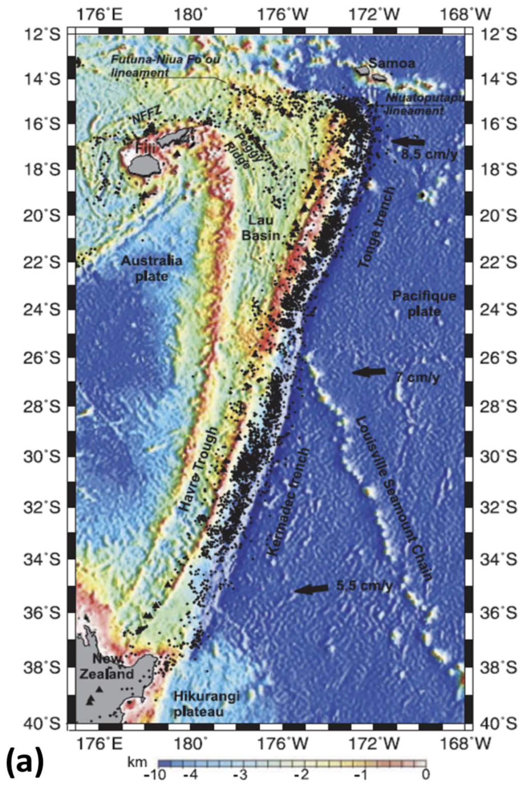
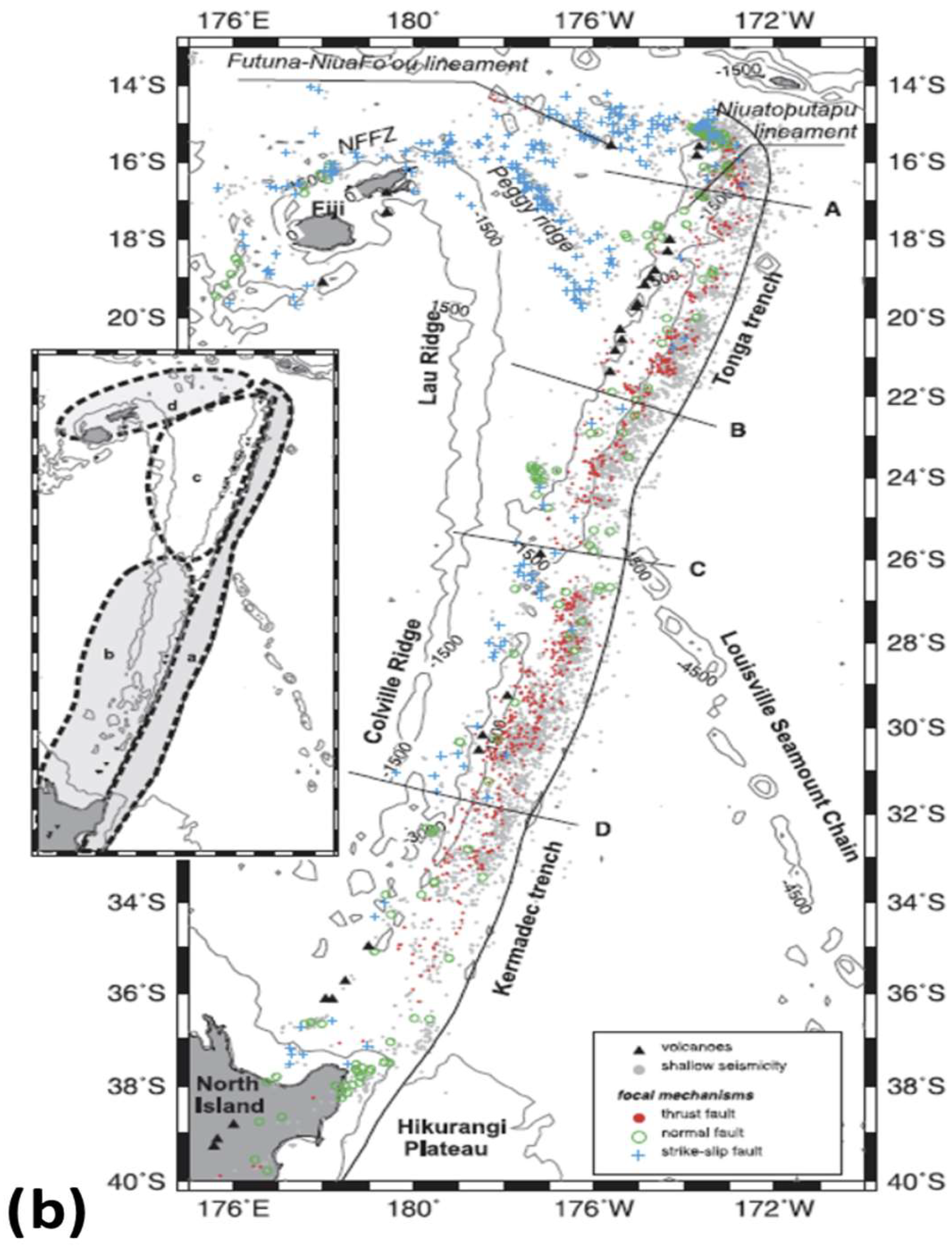
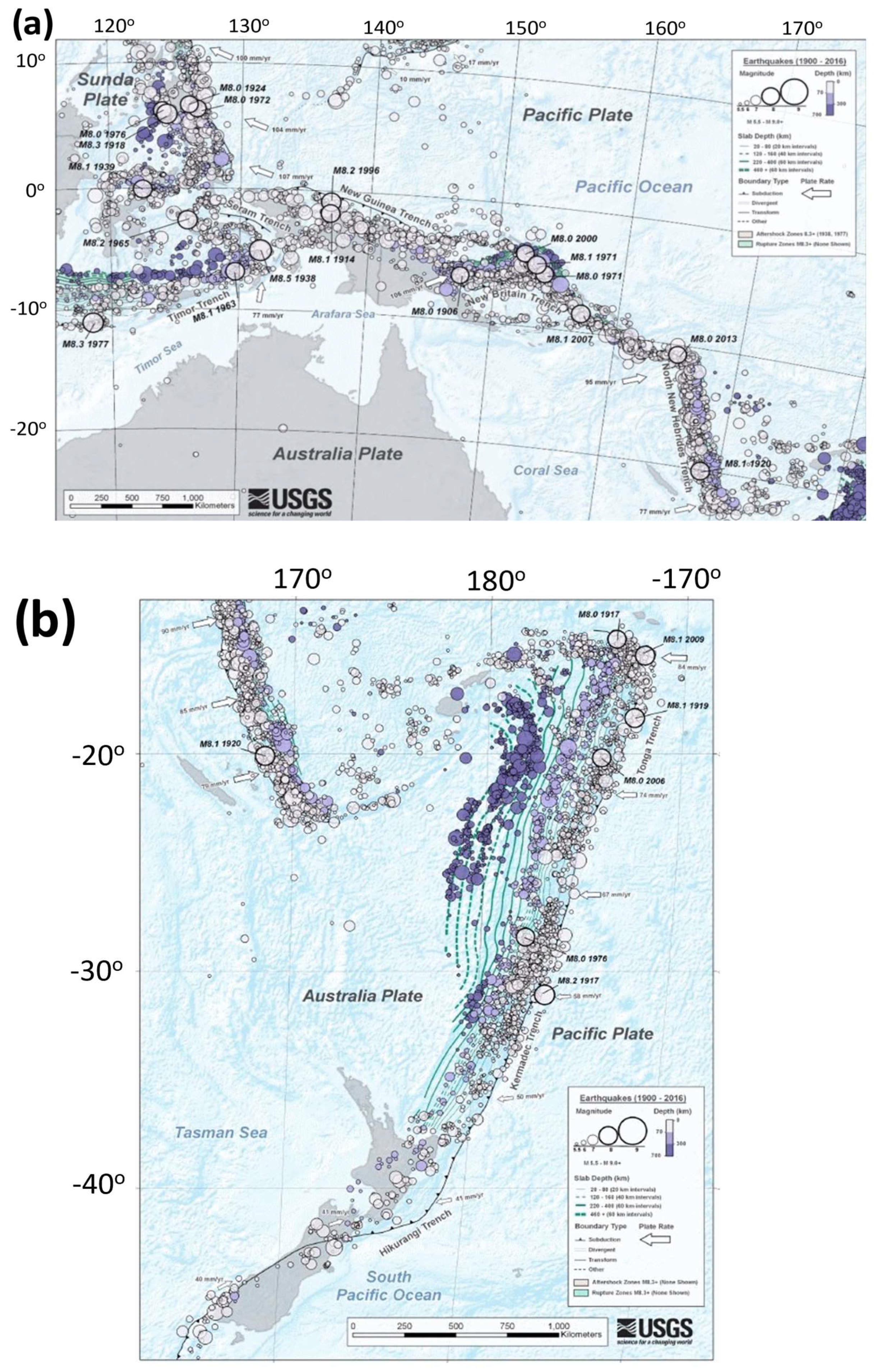
2.1. Tectonics

The South Pacific zone is a significant part of the intertropical convergence zone, which is the largest and most important convergence zone situated near the equator and extending east–west. Spanning from the Western Pacific, located at the maritime continent, towards French Polynesia, and as far as the Cook Islands (at 160°W, 20°S), it comprises a chain of active volcanoes and is affected by frequent strong EQs (Figure 2).
The northern margin of the Australia–Pacific plate boundary (Figure 2a) extends over a distance of more than 4000 km, spanning from the Sunda (Java) trench in the west to the Solomon Islands in the east, and has produced 13 EQs of M7.5+ since 1900. Moving towards the eastern margin of the Australia plate (Figure 2b) there is an oceanic transform, the Macquarie Ridge; two oppositely verging subduction zones, Puysegur and Hikurangi; and a transpressive continental transform, the Alpine Fault through South Island, New Zealand. In this zone, more than 15 M7.5+ EQs have been recorded.

2.2. NOAA Data

The NOAA POES and MetOp satellites are placed in sun-synchronous polar orbit at altitudes between 807 and 854 km (NOAA-15, 19) and at altitudes between 817 and 824 km (MetOp A-B-C), all with inclination angles of 98.6–98.8°. NOAA-15, 18, and 19 and MetOp B and C are still operational, while NOAA-16 and 17 and MetOp A are not available nowadays (more details in https://www.ngdc.noaa.gov/stp/satellite/poes/index.html accessed on 11 March 2024). They have been launched alternatively with AM/PM orbits, where the equator-crossing time of the AM series spacecraft was changed from 07:30 am for the NOAA-15 to 10:00 am for the NOAA-17 in the descending mode. Sun-synchronous polar orbits always have the same orientation with respect to the sun. This means that the satellite flies over the region of the world approximately at the same local time (LT) and LT + 12 h each day (according to ascending and descending orbits). This allows data collection approximately at the same day hours or night hours, making sampling more uniform, and allows for distinguishing between less disturbed night data from daily data due to anthropogenic and solar activities.
The particle detectors on board these satellites are the Total Energy Detector (TED) and the Medium Energy Proton and Electron Detector (MEPED) [37]. The MEPED is composed of eight solid-state detectors which consist of two proton telescopes that monitor the flux in five energy bands in the range 30 keV to 6.9 MeV, two electron telescopes in three energy bands in the range 30 keV to 2.5 MeV, and four omnidirectional detectors sensitive to proton energies above 16 MeV. The opening angle of each electron telescope is 30°, and geometric acceptances are 0.1 cm2 sr, so the view of a telescope is at an angle of 9° with respect to the local zenith, and a second one is in the orthogonal direction. It is possible to obtain the electron rates each second. The electron detector telescopes are sensitive to proton energies between 210 keV and 2.7 MeV; consequently, the computed electron fluxes need to be corrected with the counting rates (CRs) of the proton telescopes. A full set of NOAA orbital parameters was provided every 8 s, whereas satellite latitudes and longitudes were given each 2 s. NOAA data were released in a binary format with a sample time of one second prior to 2012, when electron fluxes still had not been corrected for proton contamination. The archive record of electrons and protons was provided starting from 2012 (https://www.ncei.noaa.gov/data/poes-metop-space-environment-monitor/access/l1b/v01r00/ accessed on 11 March 2024) in the netCDF (network Common Data Form) format, with the electron flux corrections and averages for all the data every 16 s.

2.3. Selections of Seismic Events and Electron Events for a Comparison

The initial studies on any correlation between NOAA satellite data and seismic events produced no significant correlation peaks between electron bursts and EQs with M5+ (as found in [9]). It was necessary to consider M6+ EQs to obtain the first positive correlations [38] and subsequently improve them by introducing the 11-year and seasonal modulation threshold [12,39]. The EQs considered in those studies occurred mainly in the regions of Sumatra and the Philippines, and those studies were later extended to a larger area of the West Pacific [30]. In an attempt to extend the result to the many EQs in the South Pacific, this first study was performed on shallow seismic activity with M6.5+ in a rectangle delimited by a longitude between 150° and 190° and a latitude between −5° and −35°. The seismic event depths were limited to 50 km, as the crust where they had occurred was already submerged by the ocean. The considered decade-long time interval was from January 2013 to June 2023, including the same period when electron fluxes were corrected for proton contamination. A total of 61 strong seismic events were registered by the USGS catalog, and they are reported in Table S1 of the Supplementary Materials.
A completely new approach was used to select electron flux increases from NOAA satellite data. Specifically, it no longer considered single electron bursts, i.e., sudden increases in electron counting rates overcoming a threshold statistically determined [12], but only more evident phenomena of electron precipitations that occurred with some persistence. First of all, only three days per EQ were considered: the day of mainshock, the day before, and the day after. Then, days where the ap index exceeded a threshold dependent on the moment of the solar cycle, as already described in a previous publication [40], were excluded. Consequently, a total of 148 geomagnetically quiet days were selected for the electron studies. Previous analysis of electron bursts from NOAA satellites showed a significant correlation 2–3 h before the West Pacific seismic events, only for electrons detected by 0° telescope and not by 90° or omnidirectional telescopes [12]; electron pitch angles were between 30° and 80°, and between 120° and 160° for correlated electron bursts. The energy measure of the electron counting rate in the energy interval between 30 and 100 keV of past publications was replaced by the electron flux in the first energy integral from 30 keV to 2.7 MeV, as initial correlations were also observed for these measurements [12]. As well as in previous studies, only electrons escaping trapped conditions were taken into account considering something that perturbed their motion in the VABs. Therefore, trapped electrons of the external VAB were excluded by limiting the relative L-shell to 2.2, and trapped electrons of the inner VAB were excluded by considering only positions where the geomagnetic field was greater than 20.5 μT.
The VABs constitute a stable dynamical system where electrons and protons move in the vacuum around geomagnetic lines indefinitely, if not disturbed. The electron flux level along the satellite orbit portions based on the rules above was intended completely to be absorbed in the South Atlantic Anomaly (SAA) within a few hours. Consequently, the mentioned flux was somehow disturbed, escaping the VABs. However, real VABs are not in an ideal medium, and particle interactions with other particles and weak electromagnetic fields are always present, so there is always a certain number of electrons escaping from this system. The flux of these electrons is affected by the noise background, while the electron flux escaping from the VABs affected by disturbances is characterized by large fluctuations above the noise background. On average, electron fluxes between a few units and a few tens of counts/cm2 s str were always present in these regions, with fluctuation durations of tenths of seconds, and therefore were really not exceptional events occurring in the ionosphere. The new analysis consisted of searching for ionospheric perturbations much more evident in amplitude and persisting. CRs detected on the semi-orbits limited by the L-shell < 2.2 and where B > 20.5 μT were considered to follow the Poissonian model. Thus, we defined the probability of a CR being non-Poissonian. MATLAB (R2022a) was used to read netCDF files downloaded from NOAA. Then, the threshold of 300 counts with a minimum total duration of 1 min was chosen to be sure to select exceptional loss events. Thus, the considered disturbances covered large portions of the geographic space, implying a long persistence in the ionosphere as they migrate eastwards before entering the atmosphere in correspondence with the SAA. Persistent electron losses (PELs) were defined as electron fluxes overcoming at least 10 times the daily average of electron fluxes in the detection areas for a timelapse of at least one minute. They were truly huge loss events that reached thousands of counts/cm2 s str detected along satellite orbit intervals of several thousands of km.

3. Results

The study of PELs started on all the available satellites, NOAA-15, 18, and 19 and MetOp 1 and 3, during the days of the strong EQs on Kermadec (2021) and Tonga (2022). Only the NOAA-18 satellite observed electron precipitation some hours before both the mentioned EQs. Thus, a systematic analysis of PELs around the EQ times of the last ten years (Table S1 on Supplementary Materials) was performed on the NOAA-18 database.

3.1. Electron Perturbations of Kermadec and Tonga EQs

The first of two events was an M8.1 EQ that hit the Kermadec Islands on 4 March 2021, at 19:28 UTC, and was preceded a few hours before by two strong foreshocks (M7.3 and M7.4) around the same region. The second EQ, with M7.3, hit the Tonga region on 11 November 2022, at 10:48:46 UTC. Electron fluxes were initially analyzed from all the NOAA and MetOp databases considering the adjacent days to the seismic events and compared to the geomagnetic activity. Specifically, Figure 3 shows the corresponding ap and Dst geomagnetic indices, which assume significant values only on the first ten hours of March 3 and on the first three hours of 4 March 2021. For the second period, the Auroral Electrojet index reaches around 700 nT at 16:30 UTC of 11 November 2022, with the consequent increase in the geomagnetic index ap that reaches the value of 12 nT. An impact due to this small increase in geomagnetic activity could be observed in the analyzed data.
Satellite electron flux measurements were therefore analyzed looking for PELs that met the requirements specified above. Figure 4 shows the geographical distribution of the NOAA-18 trajectory on the EQ day, 4 March 2021, with the detected electron fluxes along the z axis. The measurements reveal a noisy flux constituted by numerous spikes which rarely overcome 1000 counts/cm2 s str and average less than 100 counts/cm2 s str. Two peaks of precipitating electrons at negative latitudes, around 240° and beyond in longitude, are evidenced by colored circles in Figure 4. The electron perturbation highlighted in red was observed in the ionosphere at 17:33 UTC, while the Kermadec seismic event occurred at 19:28 UTC. Then, the ionospheric recorded event anticipated the strong EQ in the Southern Pacific by 2 h and 55 min. It was observed along a descending daytime orbit of the NOAA-18 satellite and reached a flux peak of about 1500 counts/cm2 s str around −20° in latitude, being intense for at least 10° of the satellite semi-orbit. It occurred immediately westwards of the SAA with a second peak of lower maximum flux detected a few minutes before along positive latitudes. The geographical position of Kermadec EQ is also indicated by a yellow disk in Figure 4. The relative longitudes of ionospheric and tectonic events were between 60° and 100°, which means that earthquake and PEL positions of correlated events were separated by several thousands of km. As the SAA is eastward of the South Pacific area, electrons drifting eastward could pass above the epicenter positions before being detected. This was compatible with a causal connection between ionospheric and tectonic events, and the advance was estimated based on the electron drift period [40]. The concept of the electron drift period is fundamental in understanding the interaction between drifting electrons and tectonic regions. The electron drift period refers to the time it takes for electrons to traverse a specific path or orbit within the Earth’s magnetosphere. This period can vary depending on factors such as the energy of the electrons, the strength and direction of the Earth’s magnetic field, and the density of charged particles in the surrounding space. In the context of interactions with tectonic regions, electron drift periods play a crucial role in several ways: (i) timing of electron interactions, (ii) induction of electrical currents, (iii) response to seismic activity, (iv) electromagnetic signals. Overall, understanding electron drift periods, electron precipitations, and their interaction with tectonic regions offers valuable insights into the complex interplay between electromagnetic phenomena and geological processes, contributing to advancements in earthquake forecasting and seismic monitoring technologies. As the electron drift motion for the considered energies is around 30°/h, drifting electrons detected by NOAA flew over the epicentral region at a 60° difference in longitude about two hours before the detections and thus may have interacted with the tectonic region of Kermadec at least 5 h before the quake.
The 2022 Tonga EQ was one magnitude unit lower than the previous EQ, and its depth was slightly greater than the Kermadec one; see Table S1 in Supplementary Materials.
Despite the differences, in this case, a few electron loss phenomena were observed over time and in correspondence to the seismic event. Another red circle evidenced the significant electron flux peak on the eastern proximity to the epicenter, indicated by a yellow disk in Figure 5. The 3D representations of the electron flux evidenced particle loss detected not only at negative latitudes, around 230° and beyond in longitude, but also at positive latitudes. The electron perturbation highlighted in red was observed in the ionosphere at around 18:30 UTC, while the Tonga seismic event occurred at 10:48 UTC.
Then, the ionospheric recorded event followed the strong EQ in the Southern Pacific by 7 h and 42 min. It was observed along a descending daytime orbit of the NOAA-18 satellite and reached a flux peak of about 1700 counts/cm2 s str, staying intense for at least 10° of the satellite’s semi-orbit. It occurred immediately westwards of the SAA with a small flux peak detected a few minutes before along positive latitudes. Eastern-drifting electrons flew over the epicentral region indicated by a yellow disk in Figure 5 more than two hours before the detections and thus may have interacted with the tectonic region of Tonga about 5.5 h after the quake. These observations prompted an investigation considering every possible extended and persistent event of electron losses from the inner VAB around each EQ time.

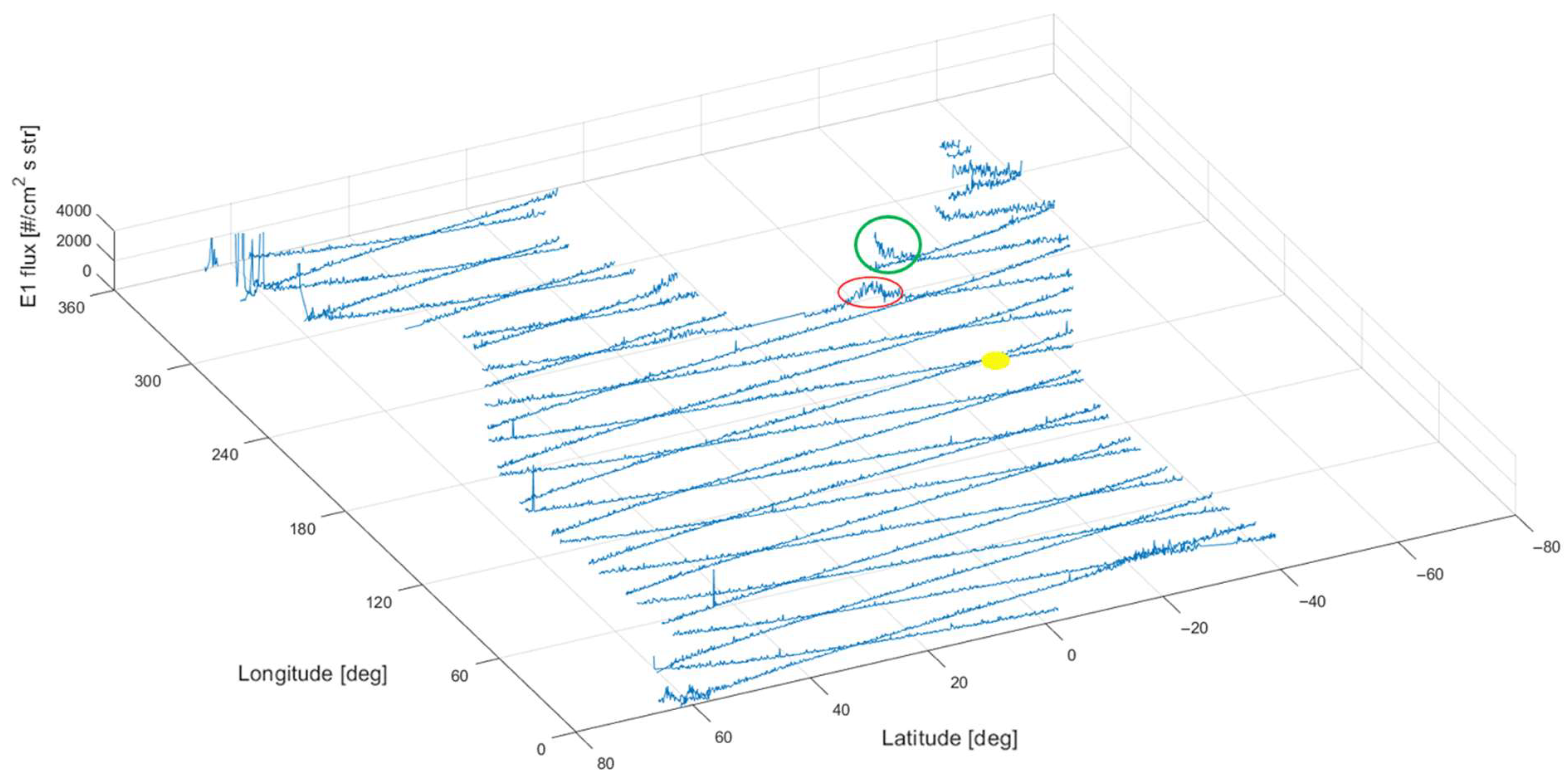
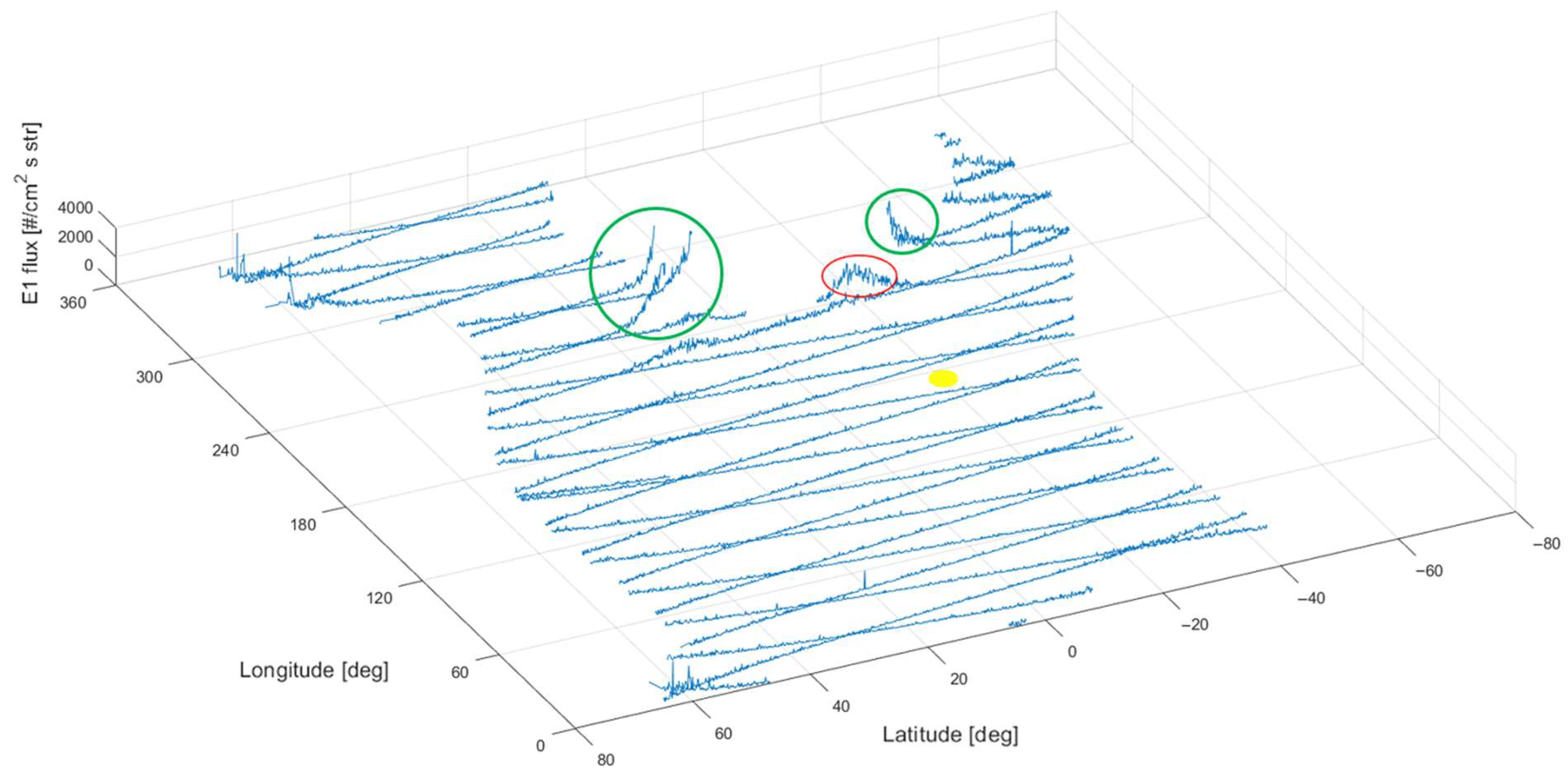
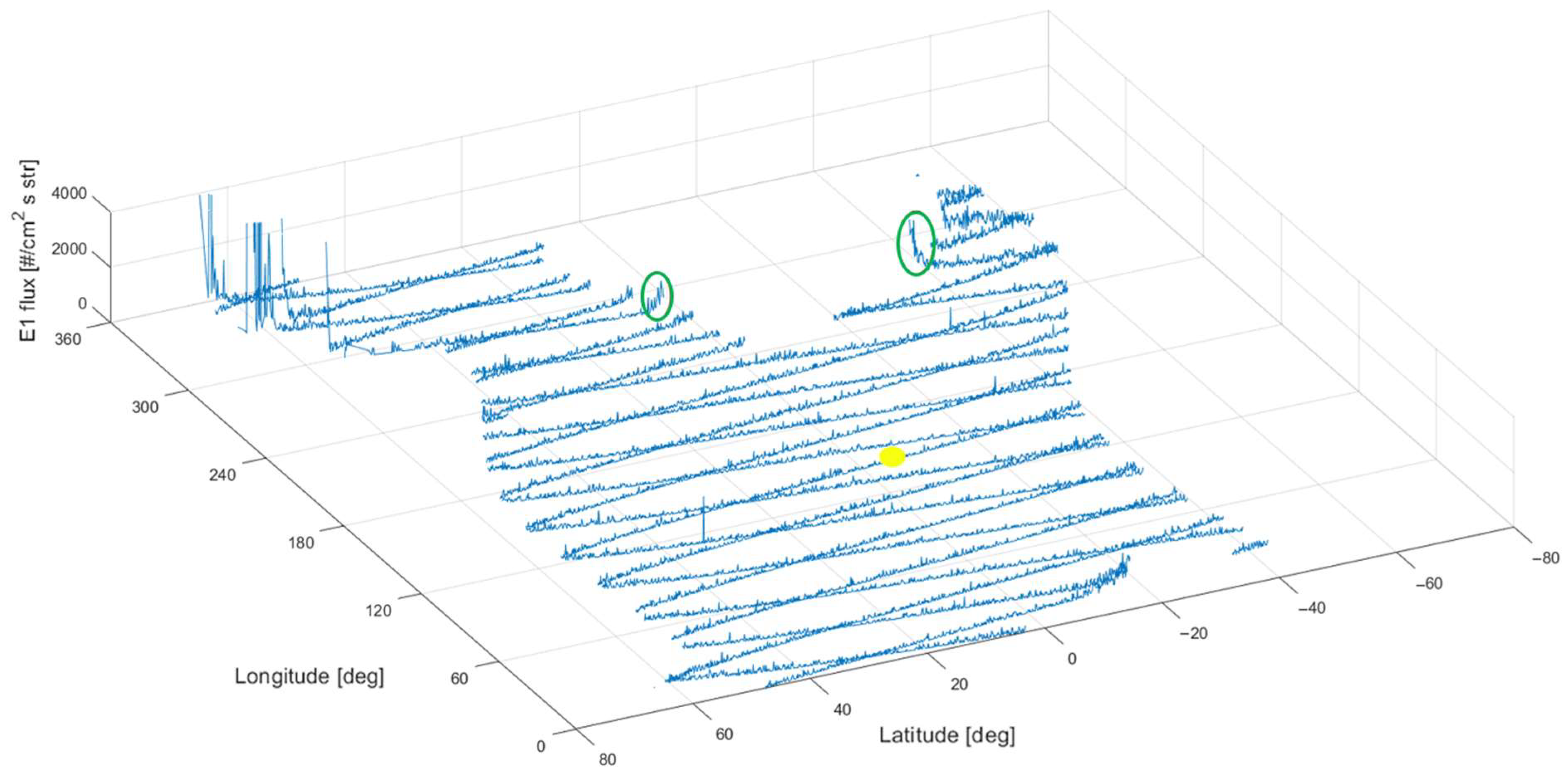
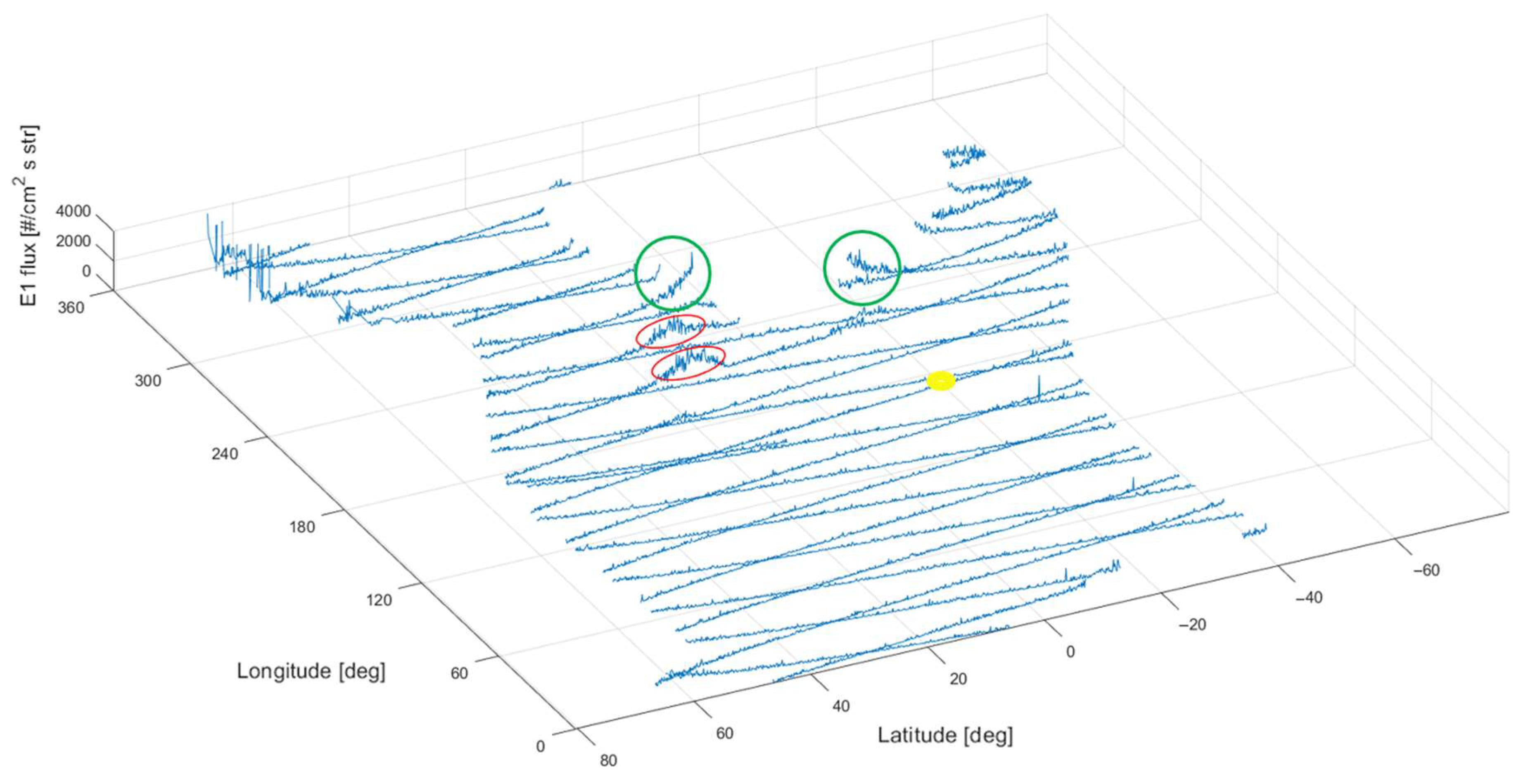
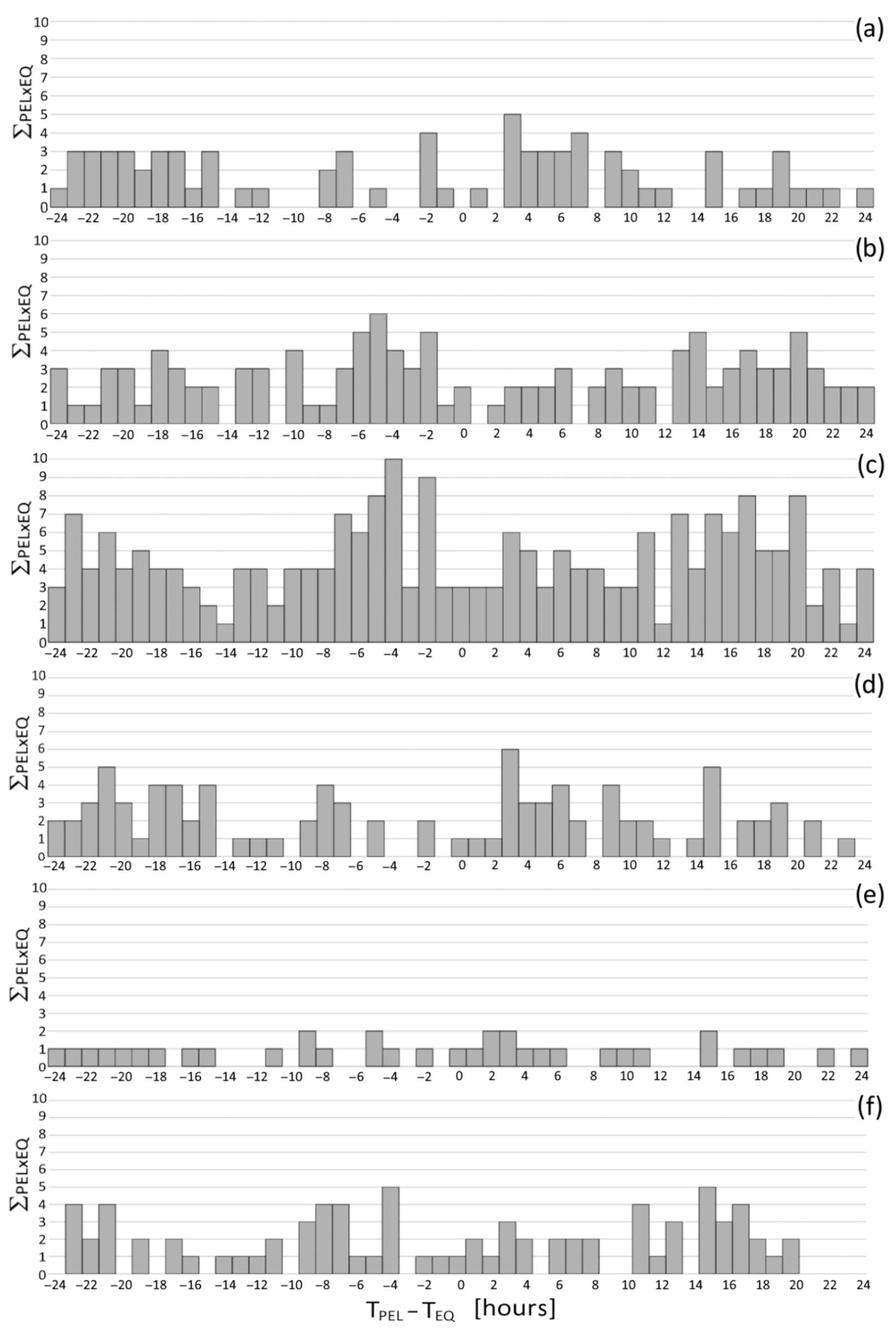
3.2. Types of Electron Perturbations

Detections occurring around the SAA border, slightly more eastward than previously, beyond 250° east, were seldom characterized by more intense electron fluxes. They were highlighted by green circles in Figure 4 and Figure 5. In the case of 19 April 2014, when an M7.5 EQ struck 70 km SW of Panguna, Papua New Guinea, high electron fluxes were detected exclusively near the SAA border (see Figure 6). They were detected along a descendent semi-orbit at longitudes of about 270° in both the southern and northern borders of the SAA, as shown by the green circles of Figure 6. Southern peak flux reached 2000 counts/cm2 s str near −40° in latitude, while northern peak flux at around 5° in latitude was half intensity. They anticipated the strong EQ in Papua New Guinea by more than 4 h. Something analogous also appeared in previous observations reported in Figure 4 and Figure 5, highlighted by green circles, where intense electron fluxes of the same kind occurred along descendent semi-orbits around 260° in longitude. Figure 5 shows only a peak around 2000 counts/cm2 s str at negative latitudes, whereas Figure 4 shows two peaks with the same intensity at both positive and negative latitudes.
As the satellites move along sun-synchronous orbits, their geographical coordinates migrate west. Thus, semi-orbits to the east will occur at times earlier. Specifically, the high fluxes measured near the SAA border of Figure 4, both at negative and positive latitudes of the descendent semi-orbit, were detected about 100 min before the respective fluxes detected at the same latitudes of the descendent semi-orbit described in Section 3.1. Therefore, they anticipated the Kermadec EQ by 4 h and 35 min. A similar detection, which followed the Tonga EQ by 5 h and 55 min, is also visible in Figure 5. High fluxes observed near the SAA were generally detected together with perturbations not detected near the SAA border as in the cases of Figure 4 and Figure 5.
Two smaller and more westwards flux increases, with respect to the above-mentioned case along descending semi-orbits, are also observed in Figure 5. They were detected along an ascendent semi-orbit at 06:10 and 06:20 UTC, a time completely different from the observation time of the descendent semi-orbit. This kind of electron loss detected along ascendent semi-orbits was generally observed at positive latitudes, and also along the subsequent westwards ascendent semi-orbits, for example on 3 December 2022, the day before the M6.8 EQ occurred in the Tonga trench area. Two large peaks of about 1500 counts/cm2 s str were observed at 06:15 and 08:00 UTC around the geographical coordinates of 10° in latitude and 240° in longitude and 20° in latitude and 220° in longitude, respectively. Electron losses were detected around 36 h before the seismic event and are shown in Figure 7 highlighted in red circles. In the same picture, PELs detected near the SAA both along ascendent and descendent semi-orbits are observed east of the first two highlighted by green circles. Thus, a variety of loss phenomena can be differentiated by the semi-orbit type, the detection on the northern or southern hemisphere, and their proximity to the SAA. Moreover, a further specification is necessary when PELs were observed both north and south of the equator along the same semi-orbit; they were assigned to the southern hemisphere.

3.3. A Comparison between Losses Observed with and without EQs

Since the reported observations of PELs during EQs occurred in Tonga and Kermadec, the EQ area was extended to all of the Southern Pacific from Papua New Guinea to New Zealand. It includes a large portion of the Ocean, with Salomon, Vanuatu, and Fiji Islands; New Caledonia; Tonga; and Samoa, where seismic events are frequently dangerous. The considered time interval was from January 2013 to June 2023; thus, the database of considered NOAA data was different from those reported in the past works [34], not only in the satellite number but also in the investigated period. The recorded PELs were constituted by precipitating electrons with bouncing altitudes that in correspondence with the SAA were lower than 100 km. From the above analysis, PELs were detected by NOAA-18 satellite westwards of the SAA, from 170° to 290° in longitude, and all the observations in each satellite semi-orbit were defined as one PEL event (PEL = 1), the time of which was the average time of the electron flux excess in that semi-orbit. The considered electron energy was a cumulative sum over a threshold declared equal to E1 = 30 keV for the 0° detector. However, due to the detector degradation, the minimum energy increased to 60 keV [41], which corresponds to electrons having a drift velocity greater than 30°/h in longitude.
How many electron loss excesses are observed when strong EQs occur in the South Pacific with respect to the case of seismic calm? This question would be addressed for electron losses from the inner VAB, and always during geomagnetically quiet days, to justify a correlation survey between two phenomena where one of them occurs more frequently. This is the case of the correlation between strong EQs and electron bursts where the electron detections occur in nearly all the considered days and their frequency is greater than that of seismic events [42]. Moreover, the area where PELs are detected, which is the same as that for the electron bursts correlated to the western (and eastern) strong seismic events due to the previously found correlation results, should be considered in addressing the request above. Therefore, the choice of the geomagnetically quiet days should be between days when no strong seismic events occur in the West (and East) Pacific too. From the definition here, it should be underlined that all the PELs are also continuous and extended electron bursts following the definition in [12], whereas events constituted by a few seconds of electron detections above the statistical threshold defined in past publications are not PELs.
For comparison, we analyzed the occurrence of PELs during periods of intense seismic activity in the Southern Pacific against those detected in periods with minimal seismic activity, spanning 60 days distributed over a decade. Given the variability in the daily frequency of PELs across years and considering a window of three days around each EQ time, two such windows were selected for each year. All selected days were characterized by low geomagnetic activity, predominantly occurring within extended geomagnetically quiet periods. From these assessments, a daily average number of PELs was defined for quiet geomagnetic periods without EQs, and the corresponding 2–3-sigma thresholds were also defined. The calculation was repeated for PELs detected along ascendent or descendent semi-orbits, southern or northern latitudes, and finally along ascendent or descendent semi-orbits around the SAA. The daily number of PELs that occurred around EQ times was averaged and found to be greater than the daily average number of PELs that did not occur around EQ times along ascendent, descendent semi-orbits, and southern latitudes, where the averages were 0.71, 1.2, and 2.2 compared to 0.30, 0.58, and 1.5, respectively. The results are shown in Figure S1a–f of Supplementary Materials and reported in Table 1. The PELs detected along northern latitudes show a 0.87 average, compared to 0.90 for the no-EQ case, line 4 of Table 1. Instead, PELs detected along both ascending and descending semi-orbits around the SAA, lines 5 and 6 of Table 1, have shown averages of 0.35 and 0.93 compared to 0.60 and 0.93 for the no-EQ case, respectively. Although significant differences are observed in the first three cases, it is necessary to understand whether these are real or due to chance. As the sample sizes were sufficiently high, with 148 for days around EQs and 60 for solar quiet days, we employed the Student’s t-test to determine if there was a statistically significant difference between the daily averages of PELs. Here the t-test was used as a parametric test of the hypothesis on two samples; it was implemented in the comparison between two sample averages. The null hypothesis H0 is that the average of PELs detected with EQs = average of PELs detected without EQs; that is, the two samples are different, in the sample averages, only due to random differences. The alternative hypothesis H1 can be formulated with the average of PELs detected with EQs > average of PELs detected without EQs, supposing a real difference between them. After the standard deviation of the two pooled samples was calculated, the statistic was distributed according to Student’s t, and the t-values and the corresponding p-values are reported in columns 6 and 7 (counting from left) of Table 1. The test was conducted on the right tail by comparing column 6 of Table 1 with the critical value of 1.645 obtained for α = 0.05. The p-values of column 7 were lower than 5%. Therefore, the null hypothesis that the two distribution averages (with or without EQs) are not different can be rejected, and the mean values of the first three PEL cases observed with EQs are significantly larger than those without EQs. We also performed a chi-square test on the same first three cases to establish the existence of a relationship between the number of PELs and the occurrence of M6.5+ EQs. The chi-square test was used as a test for independence analysis between the frequencies of 0, 1, 2, or more PEL detections for days with EQs and the expected frequencies for days without EQs. The null hypothesis H0 presupposes that there is no relation between EQ occurrence and frequencies of PEL detections, while the alternative hypothesis H1 presupposes a dependence. From the contingency matrix, it is possible to calculate the expected frequencies for independence. Then, the chi-square is calculated between observed and expected frequencies. The critical chi-square is calculated by fixing the significance level α = 0.05 and retrieving the degrees of freedom from the contingency matrix of r rows and c columns = (r − 1)(c − 1). In one of our cases for example, with EQ and no EQ, we have two rows, and with frequencies of 0, 1, 2, and 3 PELs, we have four columns; therefore, we have three degrees of freedom and a critical chi-square of 7.81. The comparison value reported in column 8 of Table 1 is obtained through the independence table. The corresponding p-value is reported in column 9 of Table 1, and the null hypothesis can be rejected. Combining the results of both statistical tests, we can affirm that the two distributions (with and without EQs) are statistically different.

3.4. The Coincidences between PELs and EQs

For a time comparison between PEL and EQ occurrences to be performed, their time series must be comparable. Therefore, both the PEL and the EQ time series were transformed into binary series by thresholds in magnitudes as specified in the previous section and in past works [10,11,12]. However, several differences were introduced to reduce the speed and difficulties of calculus. Firstly, the EQ magnitude threshold of M6.5 was chosen to reduce the number of considered seismic events to 61 (more details in Table S1 of the Supplementary Material). Moreover, the correlation was defined by filling a histogram with the products ∑⦃PEL,EQ⦄(PEL × EQ) that are equal to 1 when both PEL = 1 and EQ = 1 within the same hour and shifting the EQ times of ±1, ±2, …, ±24 h. The time step was one hour as in previous studies, even if the differences TPEL—TEQ between the EQ time TEQ and the electron perturbation time TPEL were not exactly considered. The main consequence of this new methodology was that the correlation histogram also has the value 0, corresponding to the same hour of occurrence, and thus collects a total of 49 hourly intervals; see Figure 8. Furthermore, after having chosen the EQs for the correlation, only PELs belonging to the same day, the day before, and the day after were considered. This procedure significantly decreased the time of the search for PELs. It is possible to demonstrate that the histogram of coincidence between PELs and EQs is exactly the same as that obtained if all PELs were considered. In fact, when the EQ time is shifted up to ±24 h, the coincident PELs will belong only to the previous, the same, or the past days. All the coincidences beyond ±24 h will give a zero contribution.
For what concerns the L-shell interval of PELs, it was always between L = 1.0 and L = 1.4 as for West and East Pacific cases. Furthermore, pitch angles were concentrated in intervals around 65° and 135°, with 30° ≤ α ≤ 80° and 120° ≤ α ≤ 160°, meaning that their values were mostly in the loss cone. Specifically, electrons at PEL latitudes and longitudes were confirmed to be particles escaping the trapping conditions from the inner VAB throughout the Kruglanski [43] algorithm. Finally, the geomagnetic conditions of no influence on PELs were considered, and days when the ap index was greater than the seasonal threshold for the NOAA-18 were retrieved using
                                                               ap = 13.3 + 0.8 × sen(0.37 × (D − 23,407)/365) + (2.1 − 0.1 × sen(0.37 × (D − 23,407)/365))
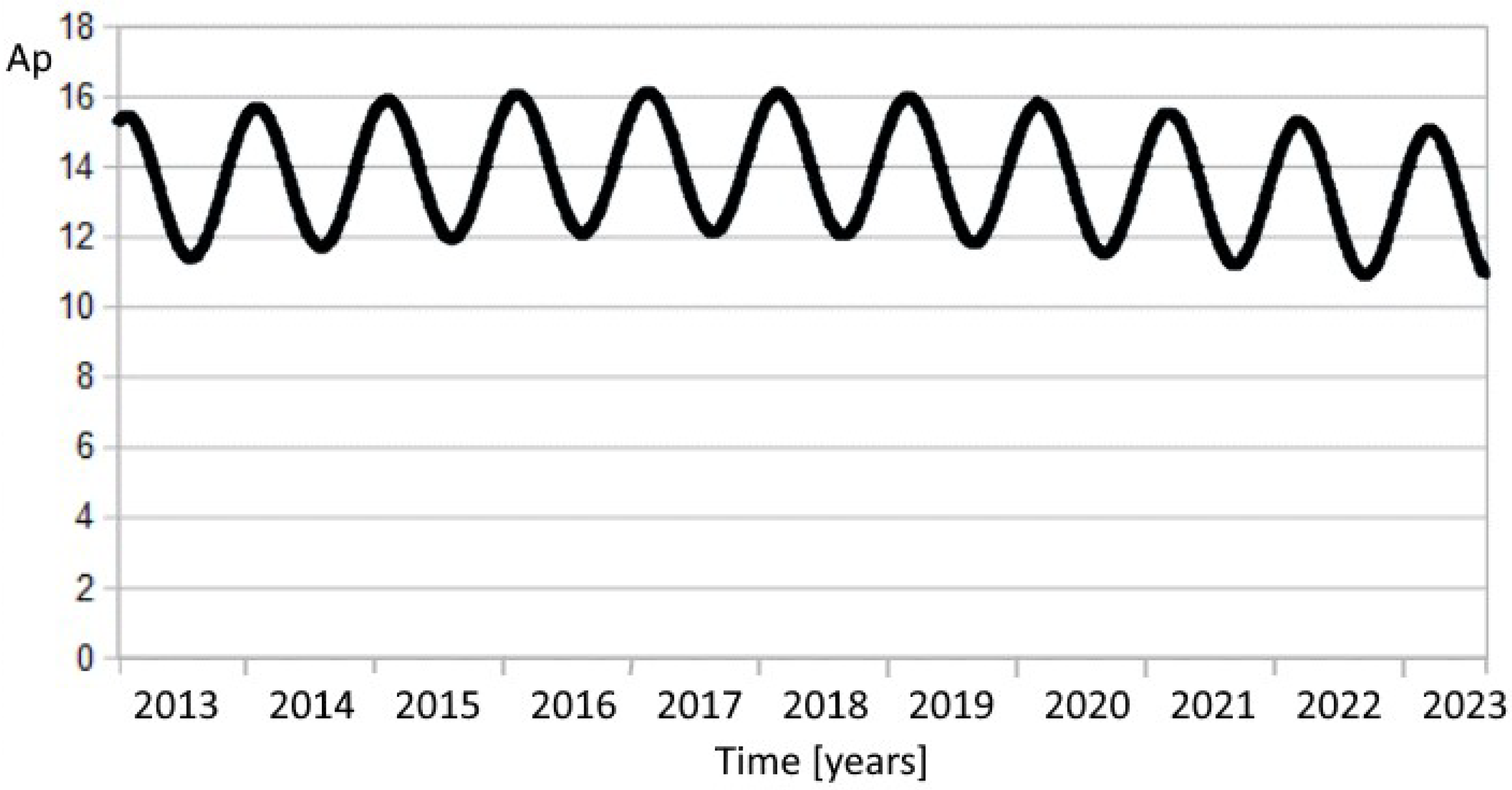
× cos(0.0172 × (D − 29,612 − 365 × (A − 2013))),
where A is the year and D is the number of days starting from 1 January 1932, when calculating the threshold. The seasonal and 22-year dependence for the ap threshold of Relation (1) was fixed in a similar way to that in past works [12] and is shown in Figure 9. Moreover, those days when a Sudden Ionospheric Disturbance (SID) occurred, or when the Dst index was greater than 30 nT, were excluded from the correlation analysis to reduce the effects of solar activity [12].
The coincidence plots between PELs and South Pacific M6.5+ EQs were calculated and are shown in Figure 8, relative to six types of semi-orbit detections by NOAA-18. They are shown for PELs detected along ascending semi-orbits in (a), along descending semi-orbits in (b), along southern latitudes in (c), along northern latitudes in (d), along ascending semi-orbits near the SAA in (e), and along descending semi-orbits near the SAA in (f). Several correlation peaks are observed from a few hours of negative time difference in (b) and (c), which means that PELs were observed before the corresponding EQs. The maximum number of 10 coincidence events was found for the time difference of 4 h, and a minor number of 9 coincidence events was found for the time difference of 2 h, as shown in Figure 8c. A lower number of six coincidence events was found for the time differences of 5 h, as shown in Figure 8b. A similar number of coincidence events was observed for the positive time difference of 3 h, as shown in Figure 8a,d, which means that PELs were observed after the corresponding EQs. The plots in Figure 8e,f show lower peaks of coincidence events due to lower statistics.

4. Discussion

The found results highlight the importance of the observed electron precipitations occurring before the earthquakes and the potential predictive nature of the ionospheric anomalies; however, the results must be taken with some caution and, moreover, must be integrated with other kinds of anomalies. An explicative model is given for the possibility of coupling between the lithosphere and the ionosphere, before formalizing the calculus of the statistical correlation.

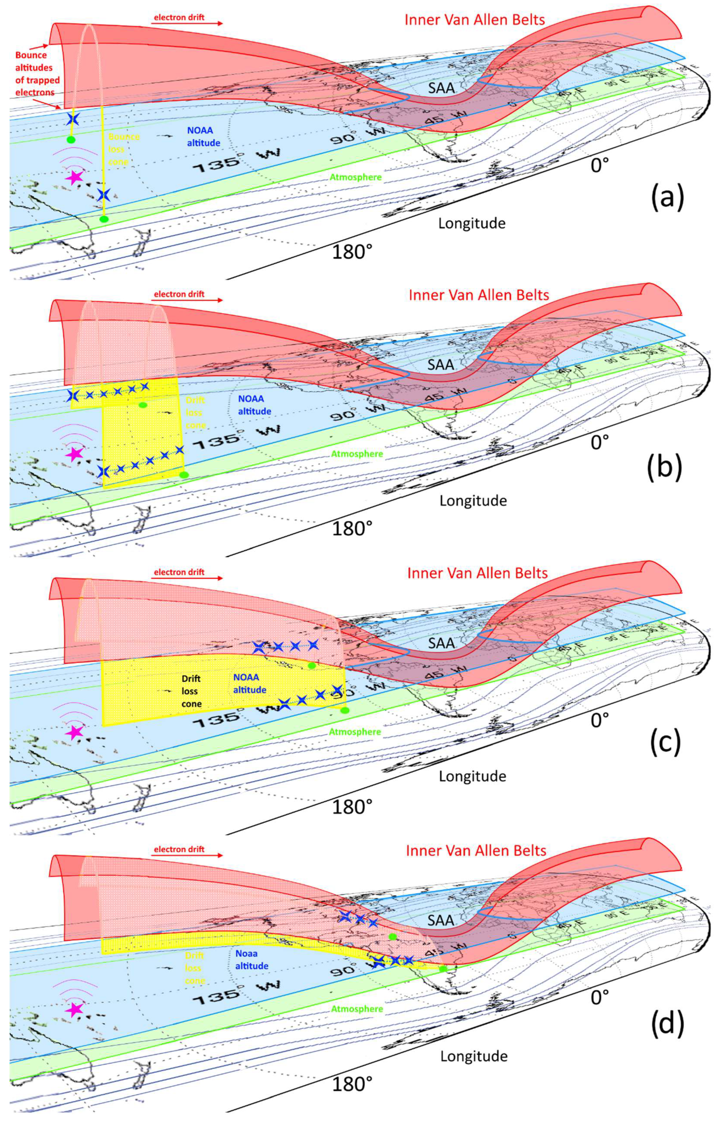
4.1. The Physical Model of Possible Long-Distance Coincidences between PELs and EQs

Figure 4, Figure 5, Figure 6 and Figure 7 show that PELs are principally detected many degrees away from the EQ epicenters, and a minor number of PELs are detected nearer the EQ epicenter, sometimes at the same latitude, sometimes also at opposite latitudes, and some other times only at opposite latitudes. Previously, a detailed study [44] explained the relation of energetic electron flux behavior at low L-shells with the SAA, evidencing that the trapped electron fluxes inside the SAA exhibit a clear local time dependence where the fluxes are maximum at night and decrease towards the east. As a possible explanation, it proposed an inward radial transport of electrons, mainly on the night side, and wave–particle interactions that could cause the dawn–dusk asymmetry in precipitation. In particular, the trapped electrons drifting eastwards close to the magnetic equator follow the paths of constant magnetic fields. So, when the magnetic field starts to decrease, approaching the SAA due to its asymmetry, the electrons descend to lower altitudes in order to conserve their magnetic moment.
Their conclusion allows us to better understand the position of PELs as detected anomalies far away from the EQ epicenters. Figure 10a–d report four cases of PELs detected at positions from near to far in relation to the EQ epicenters, where the effectivity of the physical interaction is supposed to decrease from (a) to (d). The effectivity of interaction can be thought of as the magnitude of pitch angle diffusion, which was hypothesized to have originated from magnetic pulses arriving in the ionosphere and electromagnetically coupling to charged particles [45]. Pitch angle diffusion changes particle motion, which is reflected in a bouncing altitude variation [46]. Figure 10a describes the case of a very effective interaction when electrons enter the bounce loss cone. In this case, pitch angle diffusion is so great that electron bouncing altitudes, represented in Figure 10 by yellow lower tips, reach the atmosphere, and particles are lost by scattering with gas molecules, corresponding to green circular spots. In this case, electrons have no time to drift eastwards, and losses occur at the same longitudes around the epicenter longitude. Therefore, NOAA detection, represented by a blue X in Figure 10, also occurs at the same longitude. Figure 10b describes the case of a less effective interaction when electrons enter the drift loss cone (e.g., see https://www.altfuels.org/sampex/losscone/, accessed on 11 March 2024). In this case, pitch angle diffusion is great enough that electron-bouncing altitudes reach the satellite altitude but not the atmosphere. Electrons can drift eastwards up to the bouncing altitudes that reach the atmosphere, and so they can be detected for longitudes extending from the epicenter to the loss position. Figure 10c describes the case of an even less effective interaction when electrons enter the drift loss cone. In this case, pitch angle diffusion is not great enough to reduce bouncing altitudes at the satellite altitude. Thus, electrons can drift eastwards up to the bouncing altitude reach, before the satellite altitude and more eastwards in the atmosphere. In this case, electrons can be detected for longitudes extending from the bounce crossing NOAA to the loss position. Figure 10d describes the case of little effective interaction when electrons enter the drift loss cone. In this case, pitch angle diffusion is low and slightly reduces bouncing altitudes. Therefore, electrons have to drift a lot eastwards until they approach the SAA and cross the satellite altitude just before the atmosphere. In this case, electrons can be detected for longitudes close to the west of the SAA.
Concerning the PELs observed in the northern hemisphere, as shown in Figure 7, it should be remembered that both northern and southern hemispheres are crossed due to the bouncing motion of electrons, even within the drift loss cone. Thus, a PEL detected along the semi-orbit on one side is usually detected also on the other side because the time for electrons to bounce between the northern and the southern hemispheres is less than one second. The NOAA satellite time to go from one side to the other side is around 10 min, and there is contemporary drift westward due to the sun-synchronous orbit. Therefore, if a PEL was detected on one side only, it means that the same PEL had already ended or still had not reached the satellite longitude in a time difference of 10 min, before or after depending on ascending or descending semi-orbits. For example, PELs observed in the northern hemisphere of Figure 7 on 3 December 2022, evidenced by red circles, occurred at about 100′ from each other. The absence of PELs in the southern hemisphere in both semi-orbits means that they were not observed 10′ before, and thus their duration was less than 80′. Finally, the satellite passage on the side without PEL detections preceded or followed them by several minutes.
Regarding the possible physical link, one of the first anomalous energetic particle behaviors in the ionosphere preceding a strong EQ was found and investigated by Bošková et al. [47]. They analyzed the plasma parameters considering data from the Intercosmos 24 satellite at altitudes between 2300 and 2500 km in the interval of 12–16 h before the initial shock and after the stronger aftershock of Iranian EQ 20 June 1990. An anomalous behavior of the light ionospheric ions H+ and He+ and the cold electron temperature was observed over a wide region of the northern hemisphere before the EQ, and hypothetical quasistationary electric fields of seismic origin were considered as a possible physical agent of seismo-ionospheric interactions.

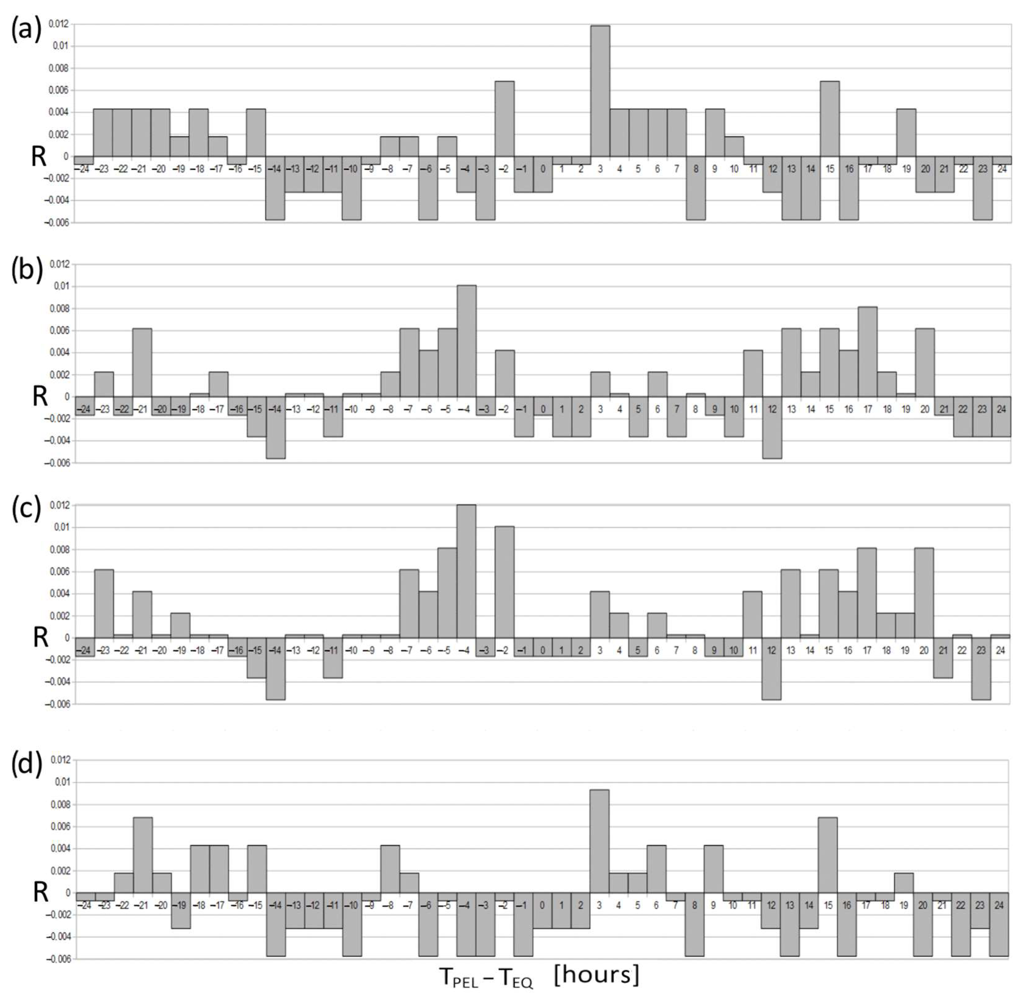
4.2. Pearson Correlations between PELs and EQs

The coincidence plots of Figure 8 gave no indication on the significance of their peaks. Furthermore, there are no true correlation plots. To obtain Pearson correlation R plots, the relation between R and the coincidence events ∑⦃PEL,EQ⦄(PEL × EQ) can be used [36]:
R = [∑⦃PEL,EQ⦄(PEL × EQ)/Nh − PPELPEQ][PEQ(1 − PEQ)PPEL(1 − PPEL)]−0.5,
where Nh is the total number of considered hours, PEQ = number of EQs/Nh is the EQ frequency, and PPEL = number of PELs/Nh is the electron perturbation frequency. Therein, the p-value can be calculated to evaluate the significance of the Pearson correlations. The total number of hours was retrieved for all days from January 2013 to May 2023 with an ap under the threshold (1). There were 2994 days, corresponding to Nh = 71,856 h. During the same period, 61 mainshocks with M6.5+ occurred in the South Pacific, so PEQ = 8.49 × 10⁻⁴. PPEL was only estimated as PELs.
PELs were identified only during days around the days of strong EQs, and during a limited number of 60 days with quiet geomagnetic conditions. As PELs used for this study were only detected during quiet geomagnetic conditions and PELs detected around the day of EQs were generally more numerous, as shown in Table 1, the PEL frequency was chosen to be the averages indicated in Table 1. They correspond to PPEL = 1.25 × 10⁻² for ascending semi-orbits, 2.43 × 10⁻² for descending semi-orbits, 6.32 × 10⁻² for southern semi-orbits, 3.75 × 10⁻² for northern semi-orbits, 2.50 × 10⁻² for ascending around SAA semi-orbits, and 3.89 × 10⁻² for descending around SAA semi-orbits.
The coincidences plotted in Figure 8e and f showed a low statistic and no high peaks. Moreover, observing that the histogram in Figure 8f shows five coincidences for −4 h in a similar way to the peak appearing in the histogram in Figure 8b, the coincidences of Figure 8e,f were summed with those in Figure 8a,b, respectively. In this way, the statistic of ascending and descending semi-orbits increased, without any distinction between PELs detected near or far from the SAA. The corresponding probabilities were PPEL = 6.32 × 10⁻² for ascending semi-orbits and 3.75 × 10⁻² for descending semi-orbits. Thus, only four histograms are plotted in Figure 11 relative to the Pearson correlations; they concern ascending semi-orbits in (a), descending semi-orbits in (b), southern latitudes in (c), and northern latitudes in (d). A peak at 3 h of time difference is observed both along ascending semi-orbits and northern semi-orbits, Figure 11a,d, which means that TPEL > TEQ and that PEL was observed 3 h after seismic events. A peak at −4 h of time difference is observed both along descending semi-orbits and southern semi-orbits, Figure 11b,c, which means that TEQ > TPEL and that PEL was observed 4 h before seismic events. A minor peak at −2 h of time difference is observed along southern semi-orbits alone, which means that PEL was also observed 2 h before seismic events for these semi-orbits.
Peaks exhibiting negative time differences signify that several PELs precede strong EQs in the South Pacific, which holds significant implications for earthquake forecasting methodologies. Moreover, these findings possess intriguing characteristics that align with causal relationships when compared to results obtained from studies involving West Pacific EQs. Specifically, EQ longitudes typically lie approximately 50° eastward of West Pacific EQ epicenters, resulting in an approximate two-hour reduction in the time it takes for them to be observed before the satellite traverses the SAA. Conversely, it is observed that the longitudes are approximately 60° west of the mean detection longitudes, indicating that PELs are detected, on average, about 2 h after the passage of electrons over the epicenters of the South Pacific. In both scenarios, it is noteworthy that the presumed disturbance in electronic motion is estimated to have occurred, on average, 6 h prior to the occurrence of EQs in the South Pacific, aligning closely with the findings for EQs in the West Pacific.
Moreover, before the application of a forecasting methodology, such as that applied by Fidani [36], a verification of the correlation peak significance should be implemented. For this purpose, correlations were calculated on 100 sets of EQs with randomized times, and p-values were retrieved along all four types of semi-orbits. Here, it is necessary to remember that each of the 61 EQs occurring at certain hours of 61 days between the beginning of 2013 and the middle of 2023 was compared with PELs that occurred from a day before to a day after the day of the EQ. This was done to reduce the time for the satellite data analysis so as to limit the correlation survey to ±24 h. Therefore, using the same set of PELs, only the hour of the EQ day was randomized inside each EQ day. This was accomplished by using 61 different random seeds between 0 and 1 multiplied by 24 h. The new EQ set was then correlated to the same PEL series. This procedure was repeated 100 times, and the number of correlation peaks that reached at least the peak magnitude of the four cases was collected. They were 20% for (a), 90% for (b), 55% for (c), and 40% for (d) in Figure 11. The results indicate that all the p-values of major peaks exceeded 20%, thus meaning that the null hypothesis fixed at 5% of cases cannot be discarded for all the correlations.

5. Conclusions

The South Pacific at the edge of the Australian Plate is a very tectonically active region. Dozens of high-magnitude EQs occur every year and are useful for a statistical study of the influence of seismic activity on the ionosphere. Specifically, the medium-energy electron precipitation phenomena from the VABs were analyzed through the particle detectors aboard NOAA-18. The main difference with respect to the past analysis is that the electron loss phenomena taken into account here were only the most intense and persistent, the so-called PELs, to distinguish them from the electron bursts, with their intensities of thousands of counts/cm2 s str maintained for several minutes. A demonstration was given that PELs are more frequent in periods of shallow EQs in the South Pacific with respect to periods of no EQs, always considering generally geomagnetically quiet days. The coincidence histogram between PELs and EQs of magnitude ≥ 6.5 was analyzed in the range ±24 h of time difference between two phenomena with hourly steps.
PELs detected around the SAA were revealed to have poor statistics; thus, the coincidence events were added to the other correspondent cases. The Pearson correlation between EQs and PELs was calculated for the four cases of PELs detected along ascending and descending semi-orbits and for PEL observations in the southern and northern hemispheres. These revealed two main peaks; the first concerned PELs anticipating strong EQs by 4 h, and the second concerned strong EQs anticipating PELs by 3 h. The peak of PELs anticipating EQs occurred for electron loss detections along descending semi-orbits and southern latitudes, whereas the peak of PELs following EQs occurred for electron loss detections along ascending semi-orbits and northern latitudes. A verification was performed on the statistical significance of the correlation peaks. The p-values of such correlations were calculated by randomly simulating EQ times. They exceeded 5% in all the cases, therefore indicating that the null hypothesis cannot be discarded. The lack of significance obtained by the test was probably due to a still low number of seismic events considered in this study.
The correlation peak of PELs forecasting EQs exhibits a time discrepancy of 4 h, which, when combined with the time taken to traverse the distances between EQ epicenters and satellite detections, amounts to approximately 6 h. This indicates that if a physical interaction occurs above EQ epicenters, it should precede EQs by roughly 6 h. This finding aligns entirely with the previously inferred advance in time of potential physical interactions, as deduced from the statistical correlation between West Pacific EQs and electron bursts, which was recently estimated to be around 6.5 h [30]. Hence, PELs and electron bursts appear to share a similar lead time concerning significant EQs. However, some caution must be exercised in interpreting their correlation with EQs from different regions.
In reality, if PELs fail to encompass short-term electron losses, electron bursts could alternatively signify the presence of prolonged precipitation, manifesting as what has been termed ‘continuous electron bursts’ [12]. The algorithm designed to identify electron bursts categorized a single detection along one semi-orbit and numerous non-contiguous electron bursts along the same semi-orbit as the same type of event. When multiple non-contiguous detections converge on a single semi-orbit, they could represent the endpoints of an enduring loss phenomenon. Hence, the correlation between electron bursts and West Pacific EQs might be attributable to both PELs and electron bursts. Consequently, a fresh correlation study between PELs and West Pacific EQs could offer further insights.
The second type of peak, featuring a positive time difference of 3 h, has not been documented in previous research. This time difference, when added to the time required to traverse the distances between EQ epicenters and satellite detections, totals one hour. Thus, if another form of physical interaction occurs above EQ epicenters, it should trail EQs by roughly one hour or, alternatively, reach the ionosphere one hour following EQ events. These two types of peaks distinguish themselves by being observed at southern latitudes along descending orbits and at northern latitudes along ascending orbits, respectively.

Supplementary Materials

The following supporting information can be downloaded at: https://www.mdpi.com/article/10.3390/rs16061059/s1, Table S1. A list of 61 earthquakes is considered for this work and taken from the USGS catalogue; Figure S1: A comparison between the daily number of PELs detected in periods with no strong EQs (blue squares), and the daily number of PELs detected in the periods with strong South Pacific EQs. Along (a) ascending semi-orbits (b) descending semi-orbits (c) southern latitudes (d) northern latitudes (e) ascending around SAA semi-orbits (f) descending around SAA semi-orbits. Averages with no EQs are represented by black dotted lines while averages with EQs are represented by red dotted lines.

Author Contributions

Conceptualization, C.F. and S.D.; methodology, C.F.; software, C.F. and M.S.; validation, C.F. and S.D.; formal analysis, C.F.; investigation, C.F. and S.D.; resources, C.F.; data curation, C.F. and S.D.; writing—original draft preparation, C.F. and S.D.; suggestions for simulation, verification and revision, A.D.S.; writing—review and editing, all authors; visualization, all authors; supervision, all authors; project administration, C.F.; funding acquisition, L.P. and A.D.S. All authors have read and agreed to the published version of the manuscript.

Funding

This research was funded by the Limadou Science + Project (ASI) and Pianeta Dinamico (Working Earth) Project (MUR).

Data Availability Statement

The NOAA-18 electron fluxes from 2013, first accessed on 31 May 2023: http://www.ngdc.noaa.gov/stp/satellite/poes/dataaccess.html. Corrections by proton contaminations were carried out using software downloaded from the Virtual Radiation Belt Observatory, first accessed on 31 May 2023: http://virbo.org/POES#Processing. The geomagnetic field was reevaluated together with L-shells on the NOAA-18 orbit using the International Geomagnetic Reference Field (IGRF-13) model, first accessed on 31 May 2023, and downloaded at http://www.ngdc.noaa.gov/IAGA/vmod/igrf.html. Geomagnetic Ap indexes and Dst variations, first accessed on 31 May 2023, were downloaded at the links https://www.ngdc.noaa.gov/geomag/data.shtml and http://wdc.kugi.kyoto-u.ac.jp/dst_final/index.html, respectively. The UNILIB libraries for calculating mirror altitudes, first accessed on 31 May 2023, were downloaded at https://www.mag-unilib.eu. Finally, EQ events were first accessed on 31 May 2023 and downloaded at https://earthquake.usgs.gov/earthquakes/search/.

Acknowledgments

The authors would like to thank Ilaria Spassiani at INGV for her insightful suggestions.

Conflicts of Interest

The authors declare no conflicts of interest.

References

  1. Imhof, W.L.; Gaines, E.E.; Reagan, J.B. High-Resolution Spectral Features Observed in the Inner Radiation Belt Trapped Electron Population. J. Geophys. Res. 1981, 86, 2341–2347. [Google Scholar] [CrossRef]
  2. Van Allen, J.A. The Geomagnetically Trapped Corpuscular Radiation. J. Geophy. Res. 1959, 64, 1683–1689. [Google Scholar] [CrossRef]
  3. Badhwar, G.D. Radiation Measurements in Low Earth Orbit: U.S. and Russian Results. Health Phys. Radiat. Saf. J. 2000, 79, 507–514. [Google Scholar] [CrossRef] [PubMed]
  4. Datlowe, D.W.; Imhof, W.L.; Gaines, E.E.; Voss, H.D. Multiple Peaks in the Spectrum of Inner Belt Electrons. J. Geophys. Res. 1985, 90, 8333–8342. [Google Scholar] [CrossRef]
  5. Voronov, S.A.; Galper, A.M.; Koldashov, S.V. Observation of high-energy charged particle flux increases in SAA region in 10 September 1985. Cosmic Res. 1989, 27, 629–631. [Google Scholar]
  6. Davis, G. History of the NOAA satellite program. J. Appl. Remote Sens. 2007, 1, 012504. [Google Scholar] [CrossRef]
  7. Aleksandrin, S.Y.; Galper, A.M.; Grishantzeva, L.A.; Koldashov, S.V.; Maslennikov, L.V.; Murashov, A.M.; Picozza, P.; Sgrigna, V.; Voronov, S.A. High-energy charged particle bursts in the near-Earth space as earthquake precursors. Ann. Geophys. 2003, 21, 597–602. [Google Scholar] [CrossRef]
  8. Sgrigna, V.; Carota, L.; Conti, L.; Corsi, M.; Galper, A.; Koldashov, S.; Murashov, A.; Picozza, P.; Scrimaglio, R.; Stagni, L. Correlations between Earthquakes and Anomalous Particle Bursts from SAMPEX/PET Satellite Observations. J. Atmos. Solar-Terr. Phys. 2005, 67, 1448–1462. [Google Scholar] [CrossRef]
  9. Fidani, C.; Battiston, R.; Burger, W.J. A study of the correlation between earthquakes and NOAA satellite energetic particle bursts. Remote Sens. 2010, 2, 2170–2184. [Google Scholar] [CrossRef]
  10. Chakraborty, S.; Sasmal, S.; Basak, T.; Chakrabarti, S.K. Comparative study of charged particle precipitation from Van Allen radiation belts as observed by NOAA satellites during a land earthquake and an ocean Earthquake. Adv. Space Res. 2019, 64, 719–732. [Google Scholar] [CrossRef]
  11. Wang, L.; Zhang, Z.; Zhima, Z.; Shen, X.; Chu, W.; Yan, R.; Guo, F.; Zhou, N.; Chen, H.; Wei, D. Statistical Analysis of High–Energy Particle Perturbations in the Radiation Belts Related to Strong Earthquakes Based on the CSES Observations. Remote Sens. 2023, 15, 5030. [Google Scholar] [CrossRef]
  12. Fidani, C. Particle precipitation prior to large earthquakes of both the Sumatra and Philippine Regions: A statistical analysis. J. Southeast Asian Earth Sci. 2015, 114, 384–392. [Google Scholar] [CrossRef]
  13. Schwarz-Schampera, U.; Botz, R.; Hannington, M.; Adamson, R.; Anger, V.; Cormany, D.; Evans, L.; Gibson, H.; Haase, K.; Hirdes, W.; et al. Cruise Report SONNE 192/2—MANGO—Marine Geoscientific Research on Input and Output in the Tonga-Kermadec Subduction Zone (Marine Geowissenschaftliche Untersuchungen zum In- und Output der Tonga-Kermadec Subduktionszone); EPIC: Auckland, New Zealand, 2007; p. 92. [Google Scholar]
  14. D’Arcangelo, S.; Bonforte, A.; De Santis, A.; Maugeri, S.R.; Perrone, L.; Soldani, M.; Arena, G.; Brogi, F.; Calcara, M.; Campuzano, S.A.; et al. A multi-parametric and multi-layer study to investigate the largest 2022 Hunga Tonga-Hunga Ha’apai eruptions. Remote Sens. 2022, 14, 3649. [Google Scholar] [CrossRef]
  15. Bonnardot, M.A.; Régnier, M.; Ruellan, E.; Christova, C.; Tric, E. Seismicity and state of stress within the overriding plate of the Tonga-Kermadec subduction zone. Tectonics 2007, 26, TC5017. [Google Scholar] [CrossRef]
  16. Genzano, N.; Filizzola, C.; Hattori, K.; Pergola, N.; Tramutoli, V. Statistical correlation analysis between thermal infrared anomalies observed from MTSATs and large earthquakes occurred in Japan (2005–2015). J. Geophys. Res. Solid Earth 2021, 126, e2020JB020108. [Google Scholar] [CrossRef]
  17. Schekotov, A.; Molchanov, O.; Hattori, K.; Fedorov, E.; Gladyshev, V.A.; Belyaev, G.G.; Chebrov, V.; Sinitsin, V.; Gordeev, E.; Hayakawa, M. Seismo-ionospheric depression of the ULF geomagnetic fluctuations at Kamchatka and Japan. Phys. Chem. Earth 2006, 31, 313–318. [Google Scholar] [CrossRef]
  18. Han, P.; Hattori, K.; Hirokawa, M.; Zhuang, J.; Chen, C.-H.; Febriani, F.; Yamaguchi, H.; Yoshino, C.; Liu, J.-Y.; Yoshida, S. Statistical analysis of ULF seismo magnetic phenomena at Kakioka, Japan, during 2001–2010. J. Geophys. Res. Space Phys. 2014, 119, 4998–5011. [Google Scholar] [CrossRef]
  19. Pierotti, L.; Fidani, C.; Facca, G.; Gherardi, F. Local earthquake conditional probability based on long term CO2 measurements. In Proceedings of the 40th GNGTS, Trieste, Italy, 27–29 June 2022; pp. 297–300. [Google Scholar]
  20. Hayakawa, M.; Kasahara, Y.; Nakamura, T.; Muto, F.; Horie, T.; Maekawa, S.; Hobara, Y.; Rozhnoi, A.A.; Solovieva, M.; Molchanov, O.A. A statistical study on the correlation between lower ionospheric perturbations as seen by subionospheric VLF/LF propagation and earthquakes. J. Geophys. Res. 2010, 115, A09305. [Google Scholar] [CrossRef]
  21. Parrot, M. The micro-satellite DEMETER. J. Geodyn. 2002, 33, 535–541. [Google Scholar] [CrossRef]
  22. Pulinets, S.A. Space technologies for short-term earthquake warning. Adv. Space Res. 2006, 37, 643–652. [Google Scholar] [CrossRef]
  23. Nemec, F.; Santolík, O.; Parrot, M. Decrease of intensity of ELF/VLF waves observed in the upper ionosphere close to earthquakes: A statistical study. J. Geophys. Res. 2009, 114, A4. [Google Scholar] [CrossRef]
  24. Li, M.; Parrot, M. Statistical Analysis of an Ionospheric Parameter as a Base for Earthquake Prediction. J. Geophys. Res. Space Phys. 2013, 118, 3731–3739. [Google Scholar] [CrossRef]
  25. Shah, M.; Jin, S. Statistical characteristics of seismo ionospheric GPS TEC disturbances prior to global Mw ≥ 5.0 earthquakes (1998–2014). J. Geodyn. 2015, 92, 42–49. [Google Scholar] [CrossRef]
  26. Sharma, G.; Nayak, K.; Romero-Andrade, R.; Mohammed-Aslam, M.A.; Sarma, K.K.; Aggarwal, S.P. Low Ionosphere Density Above the Earthquake Epicentre Region of Mw 7.2, El Mayor–Cucapah Earthquake Evident from Dense CORS Data. J. Indian Soc. Remote Sens. 2024. [Google Scholar] [CrossRef]
  27. Haider, S.F.; Shah, M.; Li, B.; Jamjareegulgarn, P.; de Oliveira-Júnior, J.F.; Zhou, C. Synchronized and Co-Located Ionospheric and Atmospheric Anomalies Associated with the 2023 Mw 7.8 Turkey Earthquake. Remote Sens. 2024, 16, 222. [Google Scholar] [CrossRef]
  28. Fu, C.C.; Lee, L.C.; Ouzounov, D.; Jan, J.C. Earth’s outgoing longwave radiation variability prior to M ≥ 6.0 earthquakes in the Taiwan area during 2009–2019. Front. Earth Sci. 2020, 8, 364. [Google Scholar] [CrossRef]
  29. Marchetti, D.; De Santis, A.; Campuzano, S.A.; Zhu, K.; Soldani, M.; D’Arcangelo, S.; Orlando, M.; Wang, T.; Cianchini, G.; Di Mauro, D.; et al. Worldwide statistical correlation of eight years of Swarm satellite data with M5.5+ earthquakes: New hints about the pre seismic phenomena from space. Remote Sens. 2022, 14, 2649. [Google Scholar] [CrossRef]
  30. Freund, F. Pre-earthquake signals: Underlying physical processes. J. Asian Earth Sci. 2011, 41, 383–400. [Google Scholar] [CrossRef]
  31. Sorokin, V.M.; Chmyrev, V.M.; Yaschenko, A.K. Electrodynamic Model of the Lower Atmosphere and the Ionosphere Coupling. J. Atmos. Solar-Terrestrial Phys. 2001, 63, 1681–1691. [Google Scholar] [CrossRef]
  32. Pulinets, S.; Ouzounov, D. Lithosphere-Atmosphere-Ionosphere Coupling (LAIC) model—An unified concept for earthquake precursors validation. J. Asian Earth Sci. 2011, 41, 371–382. [Google Scholar] [CrossRef]
  33. Hayakawa, M.; Molchanov, O.A.; NASDA/UEC Team. Summary report of NASDA’s earthquake remote sensing frontier project. Phys. Chem. Earth 2004, 29, 617–625. [Google Scholar] [CrossRef]
  34. Molchanov, O.A.; Hayakawa, M. Electromagnetics and Related Phenomena: History and Latest Results; Terra Scientific Publishing: Tokyo, Japan, 2008; p. 189. [Google Scholar]
  35. Korepanov, V.; Hayakawa, M.; Yampolski, Y.; Lizunov, G. AGW as a seismo-ionospheric coupling responsible agent. Phys. Chem. Earth 2009, 34, 485–495. [Google Scholar] [CrossRef]
  36. Fidani, C. West Pacific Earthquake Forecasting Using NOAA Electron Bursts With Independent L-Shells and Ground-Based Magnetic Correlations. Front. Earth Sci. Sect. Environ. Inform. Remote Sens. 2021, 9, 673105. [Google Scholar] [CrossRef]
  37. Evans, D.S.; Greer, M.S. Polar Orbiting Environmental Satellite Space Environment Monitor—2: Instrument Descriptions and Archive Data Documentation; Version 1.4; NOAA Technical Memorandum: Boulder, CO, USA, 2004; p. 155. [Google Scholar]
  38. Battiston, R.; Fidani, C. Correlations between NOAA Satellite Particle Bursts and Strong Earthquakes; EGU: Vienna, Austria, 2010; Volume 12, NH4.3. [Google Scholar]
  39. Fidani, C. Positive Correlation between Strong Indonesian and Philippine Region Earthquakes and NOAA Satellite Low L-shell Electron Bursts. In Proceedings of the 33th GNGTS, Bologna, Italy, 25–27 November 2014; pp. 27–34. [Google Scholar]
  40. Fidani, C. Improving Earthquake Forecasting by Correlations Between Strong Earthquakes and NOAA Electron Bursts. TAO 2018, 29, 117–130. [Google Scholar] [CrossRef]
  41. Yando, K.; Millan, R.M.; Green, J.C.; Evans, D.S. A Monte Carlo simulation of the NOAA POES medium energy proton and electron detector instrument. J. Geophys. Res. 2011, 116, A10231. [Google Scholar] [CrossRef]
  42. Fidani, C. The Conditional Probability of Correlating East Pacific Earthquakes with NOAA Electron Bursts. Appl. Sci. 2022, 12, 10528. [Google Scholar] [CrossRef]
  43. Krunglanski, M. UNILIB Reference Manual, Belgisch Instituut Voor Ruimte–Aeronomie, Which Can Be Downloaded Together to the Library from. 2003. Available online: http://www.oma.be/NEEDLE/unilib.php/ (accessed on 11 March 2024).
  44. Asikainen, T.; Mursula, K. Energetic electron flux behaviour at low L-shells and its relation to the South Atlantic Anomaly. J. Atmos. Sol.-Terr. Phys. 2008, 70, 532–538. [Google Scholar] [CrossRef]
  45. Galper, A.M.; Koldashov, S.V.; Voronov, S.A. High Energy Particle Flux Variations as Earthquake Predictors. Adv. Space Res. 1995, 15, 131–134. [Google Scholar] [CrossRef]
  46. Walt, M. Introduction to Geomagnetically Trapped Radiation; Cambridge University: Cambridge, UK, 1994; p. 168. [Google Scholar]
  47. Bošková, J.; Šmilauer, J.; Tříska, P.; Kudela, K. Anomalous behaviour of plasma parameters as observed by the intercosmos 24 satellite prior to the Iranian earthquake of 20 June 1990. Stud. Geophys. Geod. 1994, 38, 213–220. [Google Scholar] [CrossRef]
Figure 1. (a) Shallow seismicity (<50 km) map in the Australian plate and Pacific plate. (b) Distribution of the focal mechanism solutions within the upper plate, evidencing the four parts of the subduction area (from north to south): Tonga trench and Kermadec trench in a, Lau ridge in c, Colville ridge in b, and Fiji in d of the small left subfigure. Image modified from [15].
Remotesensing 16 01059 g001aRemotesensing 16 01059 g001b
Figure 2. Seismic and volcanic maps of the South Pacific convergence zone from 1900 to 2016 taken from USGS site. (a) Seismotectonic map of New Guinea Region and surrounding area (https://earthquake.usgs.gov/earthquakes/tectonic/images/newguinea_tsum.pdf, accessed on 11 March 2024); (b) seismotectonic map of the Eastern Margin of the Australia Plate (https://earthquake.usgs.gov/earthquakes/tectonic/images/emaustralia_tsum.pdf, accessed on 11 March 2024).
Remotesensing 16 01059 g002
Figure 3. ap and Dst indices during the adjacent days to the two EQs, on 3–5 March 2021 (on the left) and on 10–12 November 2022 (on the right), from https://omniweb.gsfc.nasa.gov/form/dx1.html (accessed on 11 March 2024).
Remotesensing 16 01059 g003
Figure 4. Three-dimensional representation of the NOAA-18 electron flux with respect to the semi-orbits on 4 March 2021; PELs are evidenced by colored (green and red) circles, while the yellow disk identifies the EQ epicenter.
Remotesensing 16 01059 g004
Figure 5. Three-dimensional representation of the NOAA-18 electron flux along the satellite semi-orbits on 11 November 2022; PELs are evidenced by colored (green and red) circles, while the yellow disk identifies the EQ epicenter.
Remotesensing 16 01059 g005
Figure 6. Three-dimensional representation of the NOAA-18 semi-orbits on 19 April 2014; PELs are evidenced by colored circles (see text for their meaning), while the yellow disk identifies the EQ epicenter.
Remotesensing 16 01059 g006
Figure 7. Three-dimensional representation of the NOAA-18 semi-orbits on 3 December 2022; PELs are evidenced by colored circles (see text for their meaning) while the yellow disk identifies the EQ epicenter.
Remotesensing 16 01059 g007
Figure 8. Histograms of correlation coincidences for PELs detected in 2013–2023 along (a) ascending semi-orbits; (b) descending semi-orbits; (c) southern latitudes; (d) northern latitudes; (e) ascending semi-orbits around SAA; (f) descending semi-orbits around SAA.
Remotesensing 16 01059 g008
Figure 9. The plot of Relation (1) that shows how the seasonal dependence of the geomagnetic activity is considered in the electron loss phenomena from the inner VABs. Twenty-two years of Sun activity is also shown with a precise phase; note that the maximum threshold coincides with the descendent intensity of the solar activity.
Remotesensing 16 01059 g009
Figure 10. The model of the correlation between EQs and PELs for long-distance positions between PEL detention points and EQ epicenters. Electrons enter the bounce loss cone in (a) and the drift loss cone in (bd). Red surface represents the set of trapped electron trajectories at a given L-shell. Yellow represents disturbed electrons entering the drift loss cone which are escaping the trapped conditions at the same L-shell. The lower tips of yellow trajectories are the bouncing points after disturbances acting above the future EQ epicenters. Blue Xs represent the disturbed electrons crossing the NOAA altitude, while green circles the electron absorption points in the atmosphere. The pink stars represent the EQ epicentre.
Remotesensing 16 01059 g010
Figure 11. Histograms of Pearson correlations for PELs detected along (a) ascending semi-orbits both around and far from the SAA, (b) descending semi-orbits both around and far from the SAA, (c) southern latitudes and (d) northern latitudes. Negative time differences indicate PELs anticipating EQs, while positive ones indicate PELs following EQs.
Remotesensing 16 01059 g011
Table 1. A comparison between the daily number of PELs observed around the time of strong EQs and without any EQ occurrence, during geomagnetically quiet days. Average indicates the daily average, while STD is the standard deviation. Also, the t-test and chi-square test are shown for the first three cases, reporting critical t (tc), critical χ (χc), and p-values.
Daily ResultsPEL Average without EQsPEL STD without EQsPEL Average with EQsPEL STD with EQst-Statistic
(T-Test 0.05 tc = 1.645)
T-Test p-ValueChi-Square 0.05 (DF) (χc)Chi-Square p-Value
Ascending semi-orbits0.300.560.710.713.970.000049(3) (7.81) 18.160.000407
Descending semi-orbits0.580.871.180.954.210.000019(4) (9.49) 26.440.000026
Southern latitudes1.511.182.181.233.600.000198(5) (11.07) 15.530.008322
Northern latitudes0.901.000.871.00----
Ascending around SAA0.600.660.350.52----
Descending around SAA0.930.580.830.60----
Disclaimer/Publisher’s Note: The statements, opinions and data contained in all publications are solely those of the individual author(s) and contributor(s) and not of MDPI and/or the editor(s). MDPI and/or the editor(s) disclaim responsibility for any injury to people or property resulting from any ideas, methods, instructions or products referred to in the content.

