

Enhancing Image Alignment in Time-Lapse-Ground-Penetrating Radar through Dynamic Time Warping
by

Jiahao Wen
1,
Tianbao Huang
2,
Xihong Cui
3,
Yaling Zhang
1,
Jinfeng Shi
1,
Yanjia Jiang
1,
Xiangjie Li
1 and
Li Guo
1,* 1
State Key Laboratory of Hydraulics and Mountain River Engineering, College of Water Resource and Hydropower, Sichuan University, Chengdu 610065, China
2
College of Water Conservancy & Architectural Engineering, Shihezi University, Shihezi 832000, China
3
State Key Laboratory of Earth Surface Processes and Resource Ecology, Faculty of Geographical Science, Beijing Normal University, Beijing 100875, China
*
Author to whom correspondence should be addressed.
Remote Sens. 2024, 16(6), 1040; https://doi.org/10.3390/rs16061040
Submission received: 26 January 2024
/
Revised: 8 March 2024
/
Accepted: 13 March 2024
/
Published: 15 March 2024
(This article belongs to the Special Issue Ground Penetrating Radar (GPR) Applications in Earth, Moon and Planetary Exploration)
Abstract
:Ground-penetrating radar (GPR) is a rapid and non-destructive geophysical technique widely employed to detect and quantify subsurface structures and characteristics. Its capability for time lapse (TL) detection provides essential insights into subsurface hydrological dynamics, including lateral flow and soil water distribution. However, during TL-GPR surveys, field conditions often create discrepancies in surface geometry, which introduces mismatches across sequential TL-GPR images. These discrepancies may generate spurious signal variations that impede the accurate interpretation of TL-GPR data when assessing subsurface hydrological processes. In responding to this issue, this study introduces a TL-GPR image alignment method by employing the dynamic time warping (DTW) algorithm. The purpose of the proposed method, namely TLIAM–DTW, is to correct for geometric mismatch in TL-GPR images collected from the identical survey line in the field. We validated the efficacy of the TLIAM–DTW method using both synthetic data from gprMax V3.0 simulations and actual field data collected from a hilly, forested area post-infiltration experiment. Analyses of the aligned TL-GPR images revealed that the TLIAM–DTW method effectively eliminates the influence of geometric mismatch while preserving the integrity of signal variations due to actual subsurface hydrological processes. Quantitative assessments of the proposed methods, measured by mean absolute error (MAE) and root mean square error (RMSE), showed significant improvements. After performing the TLIAM–DTW method, the MAE and RMSE between processed TL-GPR images and background images were reduced by 96% and 78%, respectively, in simple simulation scenarios; in more complex simulations, MAE declined by 27–31% and RMSE by 17–43%. Field data yielded reductions in MAE and RMSE of >82% and 69%, respectively. With these substantial improvements, the processed TL-GPR images successfully depict the spatial and temporal transitions associated with subsurface lateral flows, thereby enhancing the accuracy of monitoring subsurface hydrological processes under field conditions.
1. Introduction
Ground-penetrating radar (GPR) is a non-invasive geophysical method that emits high frequency electromagnetic waves into the ground [1]. These waves propagate the subsurface and reflect off interfaces between materials with contrasting relative permittivities. Part of the electromagnetic energy is then reflected to the surface, where it is captured by a receiving antenna, and the remainder continues to propagate downward until it dissipates [2]. Analysis of the returned signal travel times and amplitudes yields insights into the subsurface structure and characteristics [3,4]. With its capability for precise, non-destructive examination, GPR is extensively utilized in identifying the spatial positions of subterranean features [5,6,7,8], delineating subsurface stratigraphy [9,10,11], and assessing the physical properties of buried objects [1,12,13,14].
These studies have predominantly focused on the examination of static subsurface structures using GPR, while research into dynamic subsurface processes and their interplays with subsurface structures remains relatively inadequate. It is known that relative permittivity is sensitive to variations in moisture content in the subsurface, and that even minimal changes can significantly affect GPR reflections [15]. Therefore, there are emerging studies that have employed GPR with a time lapse (TL) detection manner to conduct repeated in-situ surveys of specific sites, which yield a series of GPR images tracking subsurface hydrological processes in these areas [16]. By directly differencing the TL-GPR images from the background image (e.g., the initial image collected at the beginning of the TL survey), information on the dynamics of subsurface hydrological processes, such as infiltration, preferential flow, and soil moisture distribution, can be unraveled [17]. Successful applications include mapping the path of subsurface lateral flow [9,16,18,19,20], monitoring infiltration into soil-mantled hillslopes [21,22,23,24,25] and inversion of soil water content [26,27,28].
In theory, the signal differences between repeated images obtained via TL detection could pinpoint subsurface areas with changes in soil moisture [10]. However, under real-world conditions, especially in hilly areas, factors such as surface microtopography, slope, and land cover significantly challenge the attainment of repeated GPR measurements along identical survey lines, leading to geometric mismatch among TL-GPR images [16,20]. Moreover, this geometric mismatch also generates signal differences when differencing TL-GPR images, which are difficult to distinguish from those triggered by actual changes in soil moisture [20]. That is to say, the signal differences among TL-GPR images can be attributed to both subsurface hydrological processes and geometric mismatch during field surveys. This issue constrains the precise identification of subsurface flow pathways and accurate monitoring of the infiltration process in the field [16,26].
Preceding efforts to address the issue of geometric mismatch among TL-GPR images focused on two aspects: (1) field data collection process; and (2) data postprocessing. Regarding field data collection, for example, Truss et al. [23] employed a rotating laser positioning system integrated with GPR to secure spatial coordinates with centimeter-level precision during TL surveys. This allowed for controlled antenna dragging paths, thereby minimizing geometric mismatch among TL-GPR images. In addition, studies like Haarder et al. [18] and Nyquist et al. [20] prepared wooden frames and installed wooden poles and pegs within the survey area to control antenna movement. This manner of GPR survey maintained parallelism and uniform spacing between TL survey lines, thus ensuring the comparability of TL data and suppressing geometric mismatch. However, even with meticulous data collection procedures, geometric mismatches still arise due to variations in antenna–ground coupling [20]. Moreover, these data collection operations are time-consuming and laborious, impeding large-scale application.
Regarding data postprocessing, Biken and Versteeg [29] addressed the issue of geometric mismatch in 3D TL-GPR images by applying different time shift parameters to shift the entire image. However, the determination of these time shift parameters is contingent upon the operator’s experience. Additionally, Guo et al. [16,19] tackled geometric mismatch among TL-GPR images by using regularly spaced A-scans from a background survey line as reference traces in the horizontal direction in GPR images. They then calculated the Pearson correlation coefficients between the reference traces in the background image and the neighboring A-scans from successive TL surveys, selecting the A-scan with the highest correlation coefficient as the matching trace. Subsequently, they performed interpolation on the A-scans between the chosen traces to normalize the image and enhance geometric uniformity among TL-GPR images. This same approach was employed in the vertical direction in GPR images to further suppress geometric mismatch. Yet, this comprehensive alignment process is relatively complex and not fully automatic. Most recently, Di Prima et al. [21,22] employed a moving average filter technique to mitigate geometric mismatch. Although this method is straightforward, its effectiveness in reducing the impact of geometric mismatch has not been tested across different field conditions; there is therefore an urgent need to establish an efficient TL-GPR image alignment method to minimize false signal differences triggered by geometric mismatch, while preserving signal differences due to subsurface hydrological dynamics.
To address such a practical need, this paper introduces a dynamic time warping (DTW) and algorithm-based TL-GPR image alignment method. The DTW algorithm employs a curved time axis to establish optimal correspondences between points in the test sequence and the reference sequence [30]. Through backtracking the obtained best-matching path, the DTW algorithm identifies stretch or compression time shifts in the test sequence to match the reference sequence [31], which provides a new opportunity to enhance the correspondence between the A-scan samples in the background GPR image and the subsequent TL-GPR image, thereby limiting geometric mismatches. Because subsurface lateral flow has been found to be a main mechanism of soil water transport [32,33,34], it is taken as the research focus in this study. In this regard, forward simulation software, gprMax V3.0, is adopted to generate synthetic GPR data under diverse scenarios [35]. Subsequently, the efficacy of the proposed TL-GPR image alignment method is qualitatively and quantitatively assessed by using both simulated TL-GPR images and those gathered in the field within a hilly area. This study further enhances the TL application of the GPR method in hydrological studies under field conditions.
2. Materials and Methods
2.1. TL GPR Image Alignment Using DTW
2.1.1. The DTW Algorithm
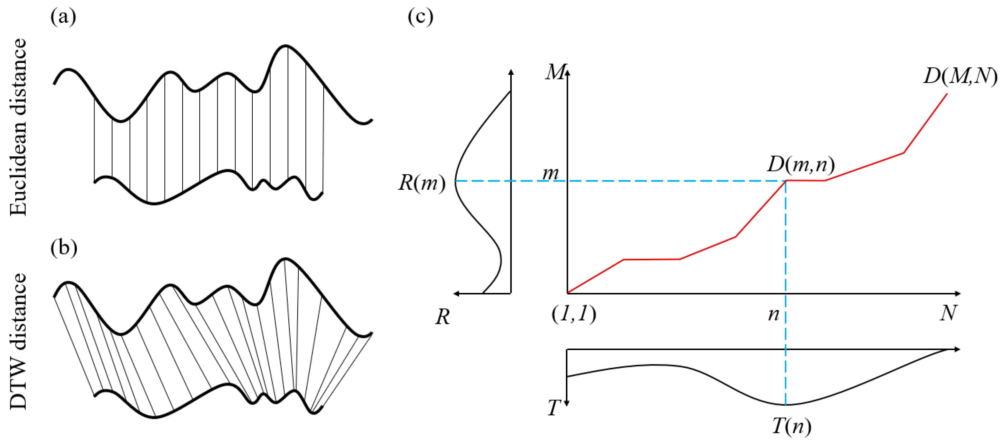
The Euclidean distance was conventionally used to gauge the similarity between two time series, which was achieved by calculating the cumulative distances of corresponding points across both series [36]. Nonetheless, as illustrated in Figure 1a, if two time series display similar overall shapes but are offset along the time axis, then using the Euclidean distance as a similarity measure might significantly bias the results. An effective alternative to this problematic approach was the use of the DTW method, which enhanced the alignment of the two time series by warping the time axis (Figure 1b) [37]. The process of determining the DTW distance involved warping the time axis to identify the minimal distance between the two time series, thereby establishing an optimal correspondence for each point pair across the time series [30]. The algorithm aimed to find the best possible pathway from the starting point to the ending point. This pathway traversed through various alignment points, aiming to minimize the cumulative distortion across its length (Figure 1c) [31,38]. The DTW algorithm was implemented as follows: suppose time series and , with lengths of m and n, respectively, where m may not be equal to n. By sorting them based on their time positions, a matrix of the size of was constructed, with each element denoted as . In the matrix , a set of adjacent elements was referred to as a warping path, denoted as , where the kth element of the path satisfies the following conditions:
- (1)
- ;
- (2)
- ;
- (3)
- for ; this element must satisfy and , then .
The dynamic programming method, relying on the cumulative distance matrix, was utilized to ascertain the warping path that produced the minimum distance between the two time series [31]. Figure 1c provides an example of a minimal warping path extending from to The expression defining the cumulative distance matrix was as follows:
where ; and . was the minimum cumulative value of the warping paths in the matrix .
2.1.2. TL-GPR Image Alignment by DTW (TLIAM–DTW)
In this study, the DTW distance derived through the DTW algorithm was used to quantify the similarity between each A-scan in TL-GPR images and its corresponding A-scan in the background GPR image. This process, referred to as the horizontal matching of A-scans, was designed to address the issues of inconsistent A-scan counts and mis-correspondence between A-scans in the background GPR image and TL-GPR images. Subsequently, based on the results of A-scan matching, the DTW algorithm was employed to determine the DTW distance and the corresponding warping path between each A-scan in the TL-GPR images and its corresponding A-scan in the background GPR image. This guided the performance of the vertical warping of the A-scans in the TL-GPR images to eliminate geometric mismatch, known as vertical warping of A-scans. Through the execution of horizontal matching and vertical warping, A-scans across TL images were sequentially undertaken to align the corresponding A-scans in the background image. During the entire process of TL image alignment, the background image remains unchanged, which is because GPR obtains TL images through repeated in-situ scanning.
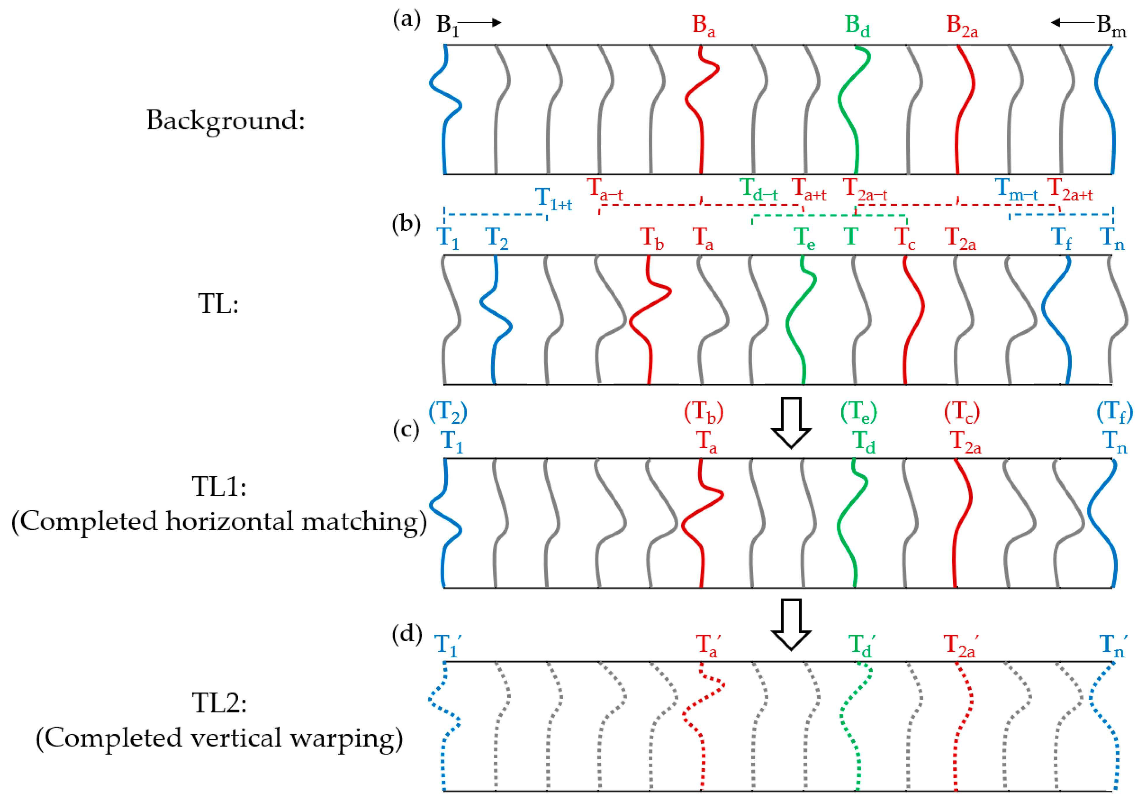
The horizontal matching of A-scans in the TL image was accomplished through a sequential process of matching marker A-scans and non-marker A-scans. Suppose that the background image (denoted as B) consists of m A-scans; and a TL image (denoted as T) consists of n A-scans, with every ath A-scan selected as a marker A-scan (noted as ) in the background image, as shown in Figure 2a,b. The remaining A-scans, meanwhile are noted as non-marker A-scans. The goal of this process is to locate the position of this marker trace in the TL image, thus completing the matching of the maker A-scans with the background image. The specific matching process was as follows:
(1) Determining the position of on the TL image and, with as the center, extend to A-scans in both the front and rear directions, denoted as and , respectively. This defined a total of 2t + 1 A-scans, which were the possible horizontal offset positions of .
(2) Using the DTW algorithm, take as the reference sequence and , , …, , …, , as the test sequences. Calculate the minimum DTW distance for each test sequence, and denote the results as , , …, , …, , , respectively.
(3) Assuming the minimum value in the results was , then (as ) is considered the test sequence most similar to the reference sequence . In other words, the A-scan in the background image corresponds to the A-scan in the TL image.
The matching process for the non-marker A-scans is consistent with the matching process for the marker A-scans. When determining the potential position of the non-marker A-scan in the TL image, it is important to note that if > (where corresponded to the A-scan in the TL image corresponding to the marker A-scan in the background image), the A-scan at in the TL image should be considered as the boundary for the possible shift range of the A-scan . After the above matching process, the horizontal matching of the TL image is completed, resulting in the acquisition of a new TL image denoted as TL1, as shown in Figure 2c.
For vertical warping of A-scans, the first A-scan in the background image serves as the reference, while its corresponding A-scan in TL1 is considered the test sequence. The test sequence might exhibit two types of changes when compared to the reference sequence: (1) false signal changes caused by geometric mismatch; and (2) signal changes due to subsurface hydrological dynamics. Thus, the vertical warping process is as follows:
(1) Using the DTW algorithm, take as the reference sequence and in TL1 as the test sequences. The DTW distance between the two sequences is calculated, and the result is recorded as . The DTW distance of each corresponding A-scan is calculated along the survey line, denoted as , , …, , …, , and the average value is obtained and denoted as .
(2) Compare the value of and , if < , there are only false signal changes due to geometric mismatch. At this time, the warping of the test sequence is completed by the DTW algorithm. Otherwise, if ≥ , there is a real signal difference caused by changes in soil water content. Then, the signal is translated as a whole to eliminate the accumulated time offset caused by the change of electromagnetic wave velocity due to the change of the relative dielectric constant of the underground medium. The overall translation of the signal is determined by a combination of the relative permittivity of the subsurface medium and the antenna center frequency.
Along the direction of antenna movement, the same warping operation is applied to each A-scan in the TL1 to eliminate the time shift issues, and the resulting TL image is noted as TL2, as shown in Figure 2d. At this point, the alignment process for TL images based on the DTW algorithm is established and named the TLIAM–DTW method.
2.2. GPR Datasets for Validation
2.2.1. Forward Simulation GPR Datasets
The effectiveness of the TLIAM–DTW was validated through simulation experiments. Plant root systems have been widely reported as channels for subsurface lateral flow migration [32,39,40], and this study therefore focused on using plant roots as the detection target for TL–GPR. All simulation experiments were conducted using the gprMax V3.0 software. This is an opensource GPR signal simulation software [35] that has been successfully applied in numerous simulation studies [41,42]. By inputting electromagnetic properties, sizes, and geometric positions of the soil and target root systems, as well as the center frequency of radar antennas, the software can generate GPR images with roots’ reflections [35]. The ideal experiment condition for the GPR survey was sandy loam with low water content and uniform spatial distribution [43]. A shrubland area in Xilingol, Inner Mongolia, China, known for its arid and semi-arid characteristics, was therefore selected for determining the simulation parameters. The roots of the Caragana microphylla Lam, typical in this region, were chosen as the simulation object [44]. The specific parameters of the medium are shown in Table 1, which is based on the results from Guo et al. [41]. The simulated experiment used a coarse root diameter of 0.02 m with a burial depth of 0.30 m. Considering the resolution and depth of coarse root detection by GPR in the study area, the center frequency of GPR antennas was set at 800 MHz with a total offset of 0.14 m and trace steps of 0.01 m.
To evaluate and corroborate the efficacy of the proposed alignment method, we established simple, single-root geometric mismatch scenarios, as well as more intricate multiple-root geometric mismatch scenarios. The software, gprMax V3.0, was employed to simulate ideal conditions, where the void space between roots and soil can act as the pathways of subsurface lateral flow. By shifting the geometric position of reflectors (e.g., root or root soil composite) within the simulation domain, the simulation was conducted to mimic the geometric mismatch occurring in the TL-GPR data acquisition. For each scenario, two different situations were simulated: the first encompassed solely geometric mismatch (hereafter referred to as Simulation 1), and the second combined geometric mismatch with real soil water content changes (hereafter referred to as Simulation 2). Simulation 1 represented the scenario with geometric mismatch alone, while Simulation 2 built upon Simulation 1 by introducing additional real signal variations. The forward simulation results for both the single-root and multiple-root scenarios were then registered to verify the effectiveness of TLIAM–DTW. According to Guo et al. [16], the maximum geometric offset in space was determined to be 0.05 m. To assess the reliability of the image alignment method in aligning TL images, ideal results without any geometric mismatch were simulated for both scenarios.
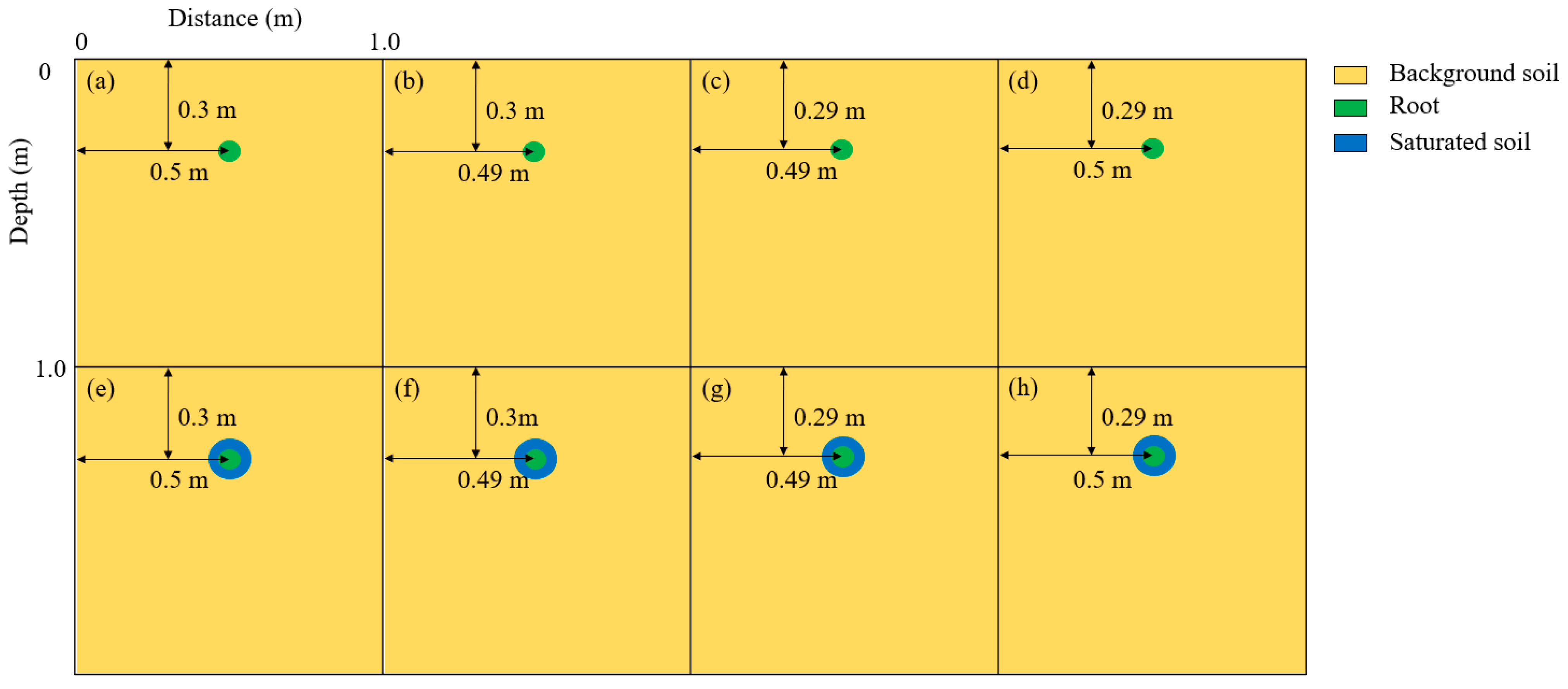
(1) Simple single-root geometric mismatch scenario: Only a single root was present in this scenario. If the geometric position of the coarse root underground was known, offsets in the horizontal and vertical directions were set with a unit of 0.01 m centered on this point. The maximum offset was set at 0.05 m. In the actual process of TL detection, the horizontal offset and vertical offset were independent of each other. Additionally, the left–right offset in the horizontal direction and the up–down offset in the vertical direction were the same. In this scenario, we only simulated the case where the root system is shifted to the left (referred to as “Lm”) and shifted upwards (referred to as “Um”). Figure 3a represents the initial situation, while Figure 3b–d demonstrate all possible offset scenarios that could occur for a single root with a geometric offset distance of 0.01 m in Simulation 1. Figure 3e–h corresponded to Simulation 2 under Simulation 1. A total of 72 (6 × 6 × 2) simulated results were obtained.
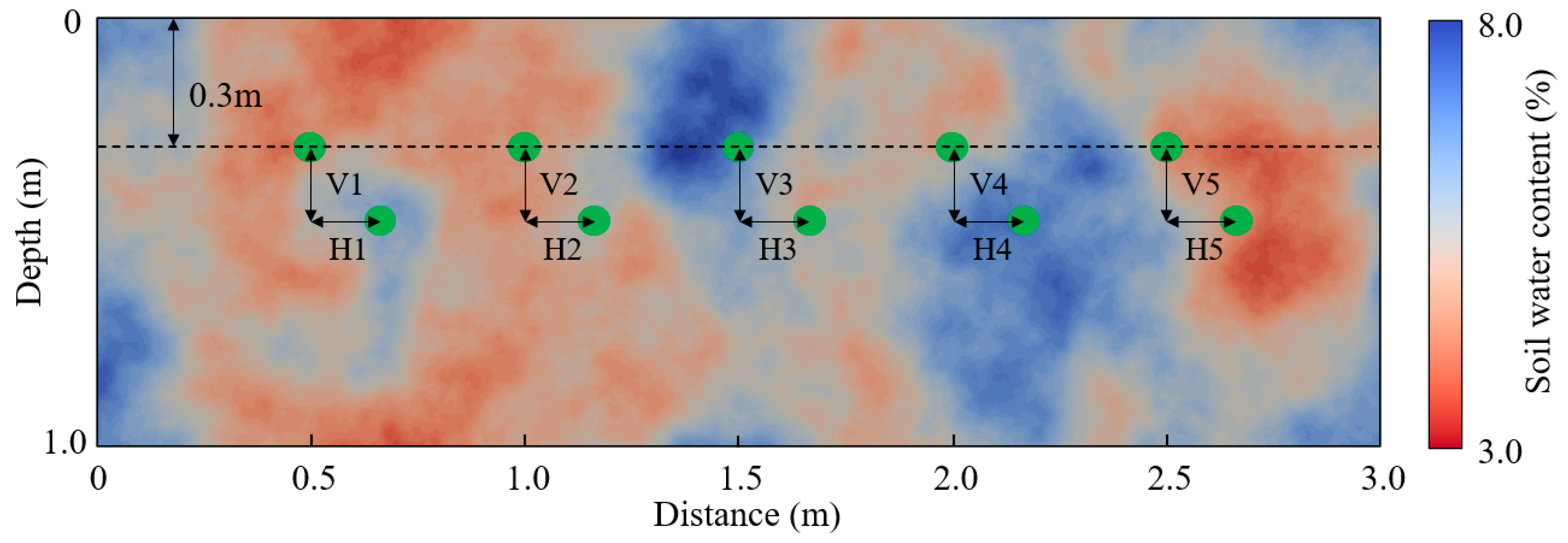
(2) Complex multiple-root geometric mismatch scenario: In natural settings, it was typical for multiple coarse roots to inhabit a given area. This scenario therefore incorporates ten roots—five stationary base roots with preset spatial positions, and five mobile roots with variable spatial positions. A gradient alteration was observed in the relative spatial positioning of the mobile roots in relation to their corresponding base roots, with variations ranging from 0–5 cm, 5–10 cm, 10–15 cm, and 15–20 cm. Table 2 presents the spatial relative positioning of each mobile root and its respective base root. During the TL detection process, it was critical to note that each mobile root’s geometric offset occurred independently, with varying degrees of deviation. Figure 4 depicts the initial setup, where base roots were spaced 0.5 m apart. In this scenario, an important assumption was introduced, with only the mobile roots experiencing a geometric offset. Nonetheless, in Simulation 2 all roots were subject to actual signal modifications. Table 3 further illustrates the geometric offset pertaining to the five mobile roots. Consequently, a total of eight simulated results (4 × 2) were obtained.
2.2.2. Field Collected TL-GPR Datasets
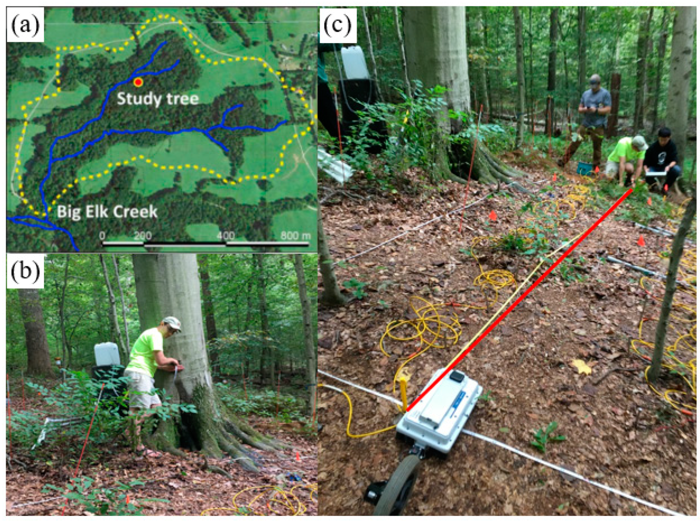
In addition to forward simulation datasets, field TL GPR data collected from a hilly area were also used to validate the TLIAM–DTW. The field GPR survey was conducted on a slope within the Fair Hill Natural Resource Management Area in northeastern Maryland, USA, on 18 September 2017 (Figure 5a). The forest litter around the base of the sample tree was not removed to enable a better representation of stemflow entering into the soil under natural conditions. Regular tap water was directed onto the tree trunk at breast height, facing downslope, using PVC tubing (Figure 5b) to simulate stemflow generation and infiltration. The tubing, connected to a water tank, maintained a flow rate of around 4 L/min. There was minimal overland flow, with occasional pooling at the tree base, where most of the stemflow seeped into the soil. A total of 100 L of water was released over 50 min, and TL data was obtained using GPR at 0 and 120 min after the completion of infiltration. The Swedish Mala GXGPR system was adopted to collect TL-GPR images along a 6.0 m survey line (indicated by the red line in Figure 5c) with an antenna frequency of 750 MHz, providing a maximum detection depth of 0.8 m. To ensure consistency of antenna movement, plastic barrels were used to anchor the ends of the survey line across different time points. A detailed description of the experiment can be found in Guo et al. [39].
2.3. GPR Data Preprocessing
The preprocessing steps for GPR image data included: (1) First arrival time extraction: the first arrival time referred to the moment when the electromagnetic wave emitted by GPR antennas reaches the ground; (2) Bandpass butterworth filter and background noise removal improving the signal-to-noise ratio; (3) Velocity analysis: the wave velocity was calculated from the relative permittivity of the soil in Table 1, using the calculation formula in Guo et al. [43]. In the field measurements, the wave propagation velocity was obtained from Guo et al. [39]; (4) Time–depth conversion: the propagation time of the electromagnetic wave was converted to actual depth using the time–distance formula; (5) Kirchhoff migration: this step aimed to remove profile image distortions caused during data acquisition; (6) Hilbert transform: converting the amplitude data of the original radar signal, which has a polarity, into energy data that only represents the strength of the reflection signal [43]; (7) Moving average filter: by using a sliding window of a given size, the average value of all energy data within the window was calculated to eliminate the influence of geometric mismatch [21].
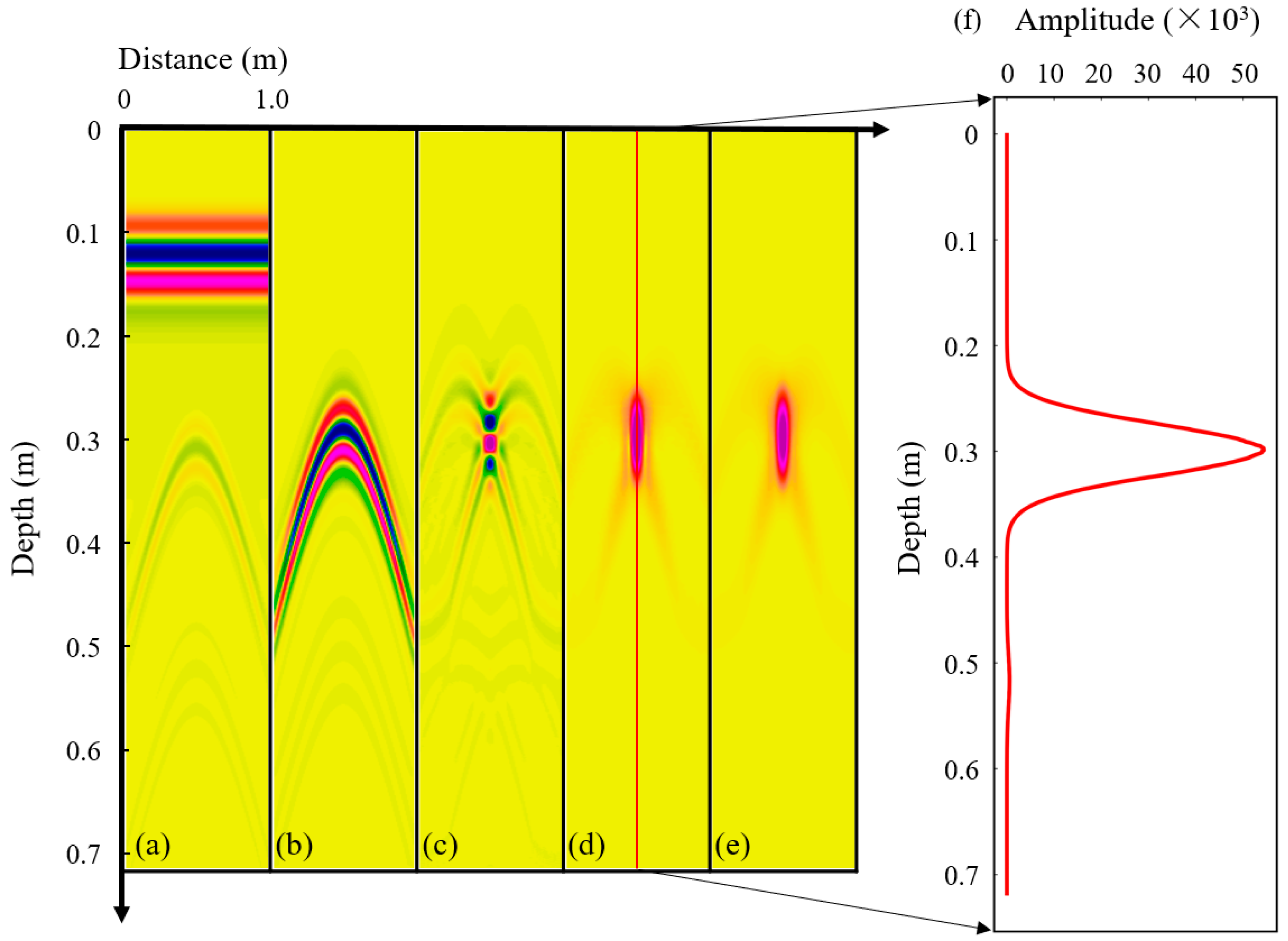
Figure 6 illustrates the processing results of the major preprocessing steps. Overall, advanced radar data processing methods significantly enhanced the quality of radar imagery. Image preprocessing was performed using Reflexw 9.5 software (Sandmeier Scientific Software, Karlsruhe, Germany). It was worth noting that the bandpass butterworth filter was only used for field-measured data preprocessing.
2.4. Quantitative Assessment of the TLIAM-DTW Method
For the preprocessed TL GPR images, the moving average filter (MAF) [21] and the TLIAM–DTW were applied for TL-GPR image alignment, followed by differencing the processed TL images with the background images. These differential results were labeled as “MAF” and “DTW”, respectively. Additionally, the direct difference between TL images without any alignment process and the background images was retained as “Direct”. The difference between the TL images (without geometric mismatch) and the background images were labeled as “Reference”, acting as the baseline for comparison. By comparing the differential results with the baseline, a qualitative assessment of each method’s strengths and weaknesses can be accomplished. Additionally, mean absolute error (MAE) and root mean square error (RMSE) were selected as quantitative measures to assess the difference between different alignment results and the ideal result:
where is the jth amplitude value of the ith A-scan in the “Reference”; is the jth amplitude value of the ith A-scan in the “Direct”, “MAF” and “DTW” respectively; m is the total number of amplitudes in the “Reference”; n is the total number of amplitudes in the “Direct”, “MAF” and “DTW” respectively.
3. Results
3.1. Performance of the TLIAM–DTW Method for Simulation Datasets
3.1.1. Analysis of Simple Single-Root Geometric Mismatch Scenario
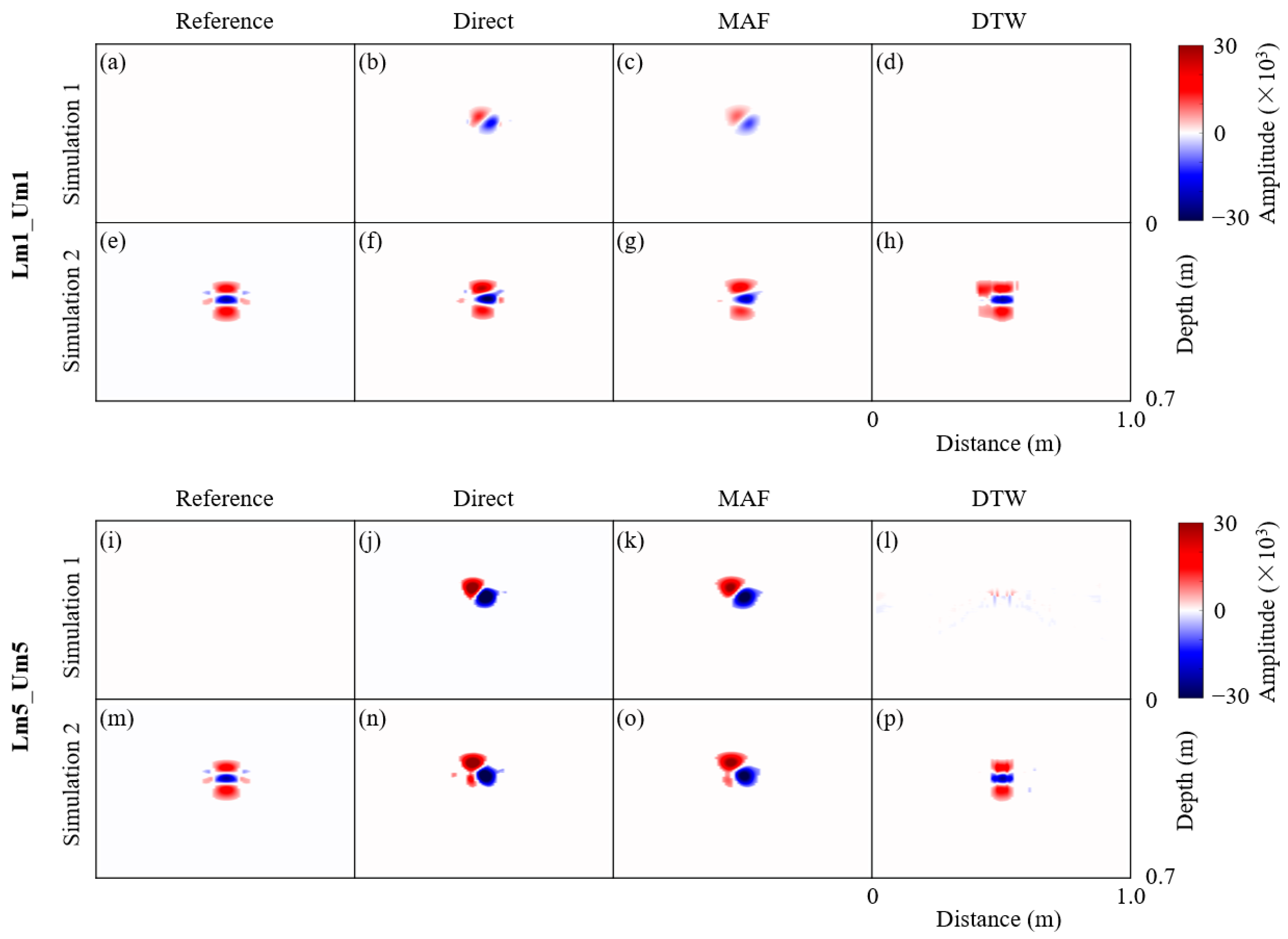
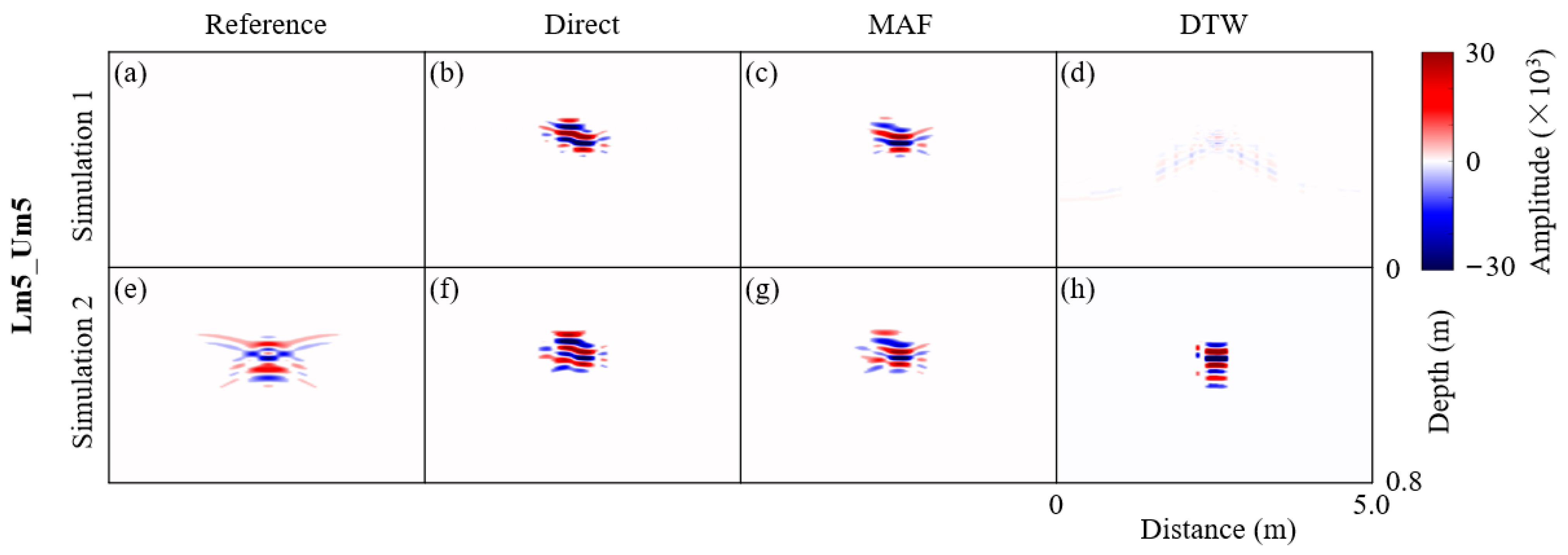
Figure 7 collectively displays the differential results after applying necessary data preprocessing and using various alignment methods to eliminate geometric mismatch issues. Only two results are shown in which the geometric mismatch is the smallest (specifically, the root is shifted 0.01 m to the left and 0.01 m upward, denoted as “Lm1_Um1”) and largest (similarly denoted as “Lm5_Um5”).
For Simulation 1 (Figure 7a–d,i–l), where no true signal variations exist under the ideal condition of no geometric mismatch, the GPR detection results along the same profile at different times should remain consistent. Therefore, the differential results between the images at different times and the background image should be zero, shown as “Reference”. However, when a geometric mismatch problem occurs, regardless of “Lm1_Um1” or “Lm5_Um5”, the “Direct” clearly shows signal discrepancies that should not be present. Furthermore, there is no significant difference between the “Direct” and “MAF”. The signal discrepancies that should not have occurred are still evident. In contrast, the “DTW” does not show significant signal discrepancies.
For Simulation 2 (Figure 7e–h,m–p), where true signal variations exist, the “Reference” shows a clear and neatly arranged red-blue-red alternating signal pattern. This phenomenon mainly occurs because the relative permittivity difference between saturated soil and background soil is much greater than the difference between root and background soil: as a result, the signal intensity in the TL image is stronger than in the background image. The interface between saturated soil and background soil is closer to the ground compared to the interface between roots and background soil, resulting in a shorter signal propagation time in the TL image [7]. With regard to the “Lm1_Um1” scene, the differences between “Reference”, “Direct”, and “MAF” are seen to be relatively small. However, in “Direct” and “MAF”, a horizontal offset is observed between red and blue signals, although the degree of offset is small. In contrast, “DTW” differential results show neatly arranged red-blue-red alternating signals, and there is no horizontal offset between the red and blue signals, indicating that the image alignment process successfully eliminates geometric mismatch. However, additional red signals that do not correspond to blue signals can be observed, indicating occurrences of mismatch during the horizontal matching process. With regard to “Lm5_Um5”, there is a noticeable difference between “Direct”, “MAF” and “Reference” and these results clearly show the geometric mismatch problem in the TL image; however, the “DTW” closely resembles the “Reference”, indicating a thorough resolution of the geometric mismatch problem in the TL image. Additionally, the appearance of additional red signals diminishes as the degree of geometric mismatch increases.
It is worth noting that, in both Simulation 1 and Simulation 2 within the “Lm5_Um5”, there is no discernible distinction between the differential results when employing either direct differencing with the background images or differencing after applying moving average filter to the TL images. Consequently, it becomes impossible to determine if these signal differences originate from genuine signal variations. This issue can significantly impact the description of subsurface lateral flow pathways using TL-GPR, which intuitively demonstrates the necessity of performing image alignment on the TL images.
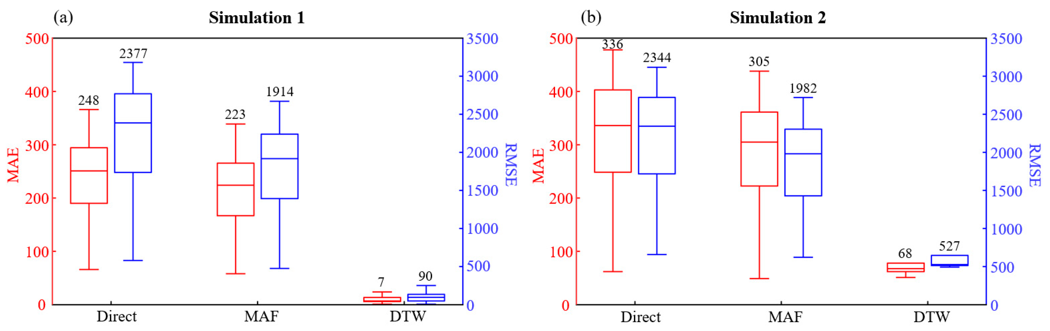
Calculating the MAE and RMSE of the “Direct”, “MAF”, and “DTW” and then comparing them to the “Reference” makes it possible to quantitatively evaluate the effectiveness of various methods for solving geometric mismatch. Based on these results, box plots were further generated for different evaluation metrics under various methods (Figure 8). From the box plots, it can be observed that, for both Simulation 1 (Figure 8a) and Simulation 2 (Figure 8b), the moving average filter only slightly reduces the impact of geometric mismatch. For Simulation 1, the MAE and RMSE decrease from 248 and 2377 to 223 and 1914, respectively. Similarly, for Simulation 2, the MAE and RMSE decreased from 336 and 2344 to 305 and 1982, respectively. However, the influence of geometric mismatch is significantly reduced after applying the TLIAM–DTW. In particular, TLIAM–DTW virtually eliminates the effect of geometric mismatch in Simulation 1: the MAE decreases from 248 to 7, reflecting a 97% decrease, while the RMSE decreases from 2377 to 90, indicating a 96% decrease. Meanwhile, the MAE in Simulation 2 drops from 336 to 68, showcasing an 80% decrease, and the RMSE decreases from 2344 to 527, representing a 78% decrease.
Based on the above analysis, the simulation results of a simple single-root geometric mismatch scenario show that the TLIAM–DTW greatly reduces the false differences caused by geometric mismatch while preserving the true differences caused by signal variations.
3.1.2. Analysis of Complex Multiple-Root Geometric Mismatch Scenario
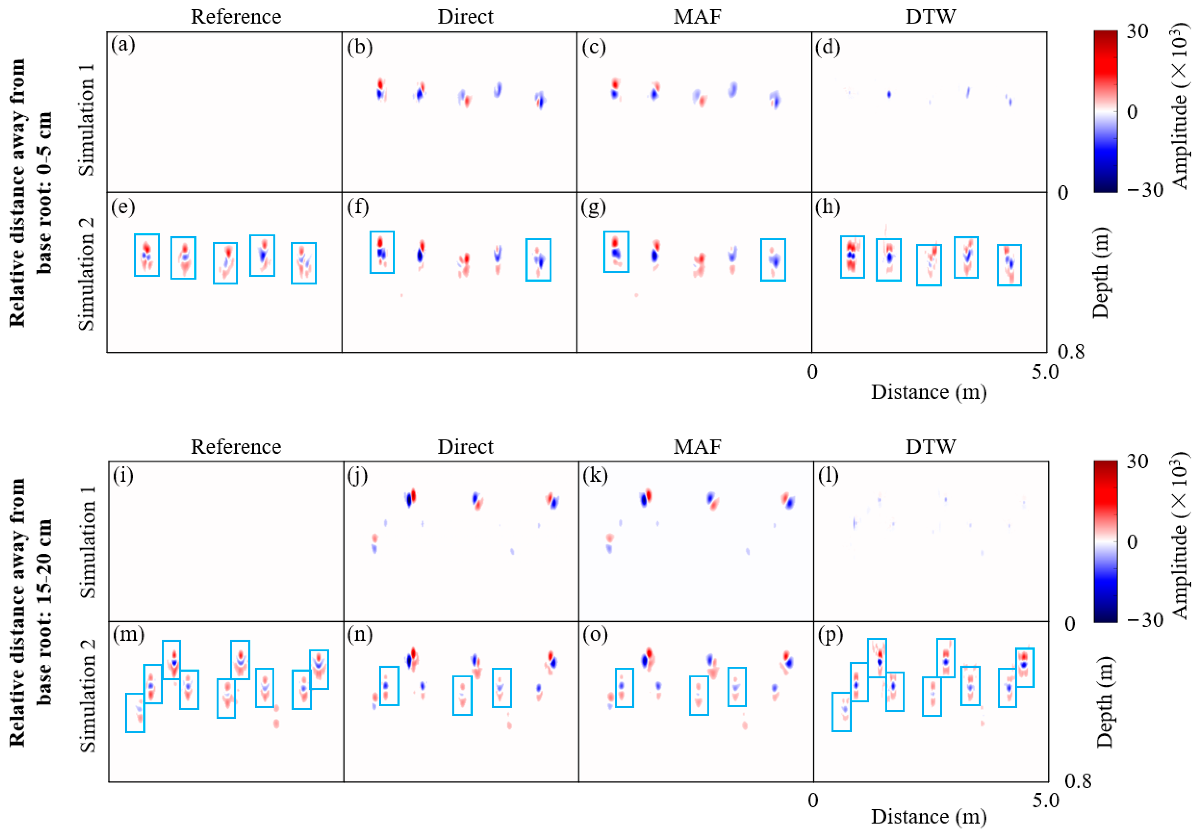
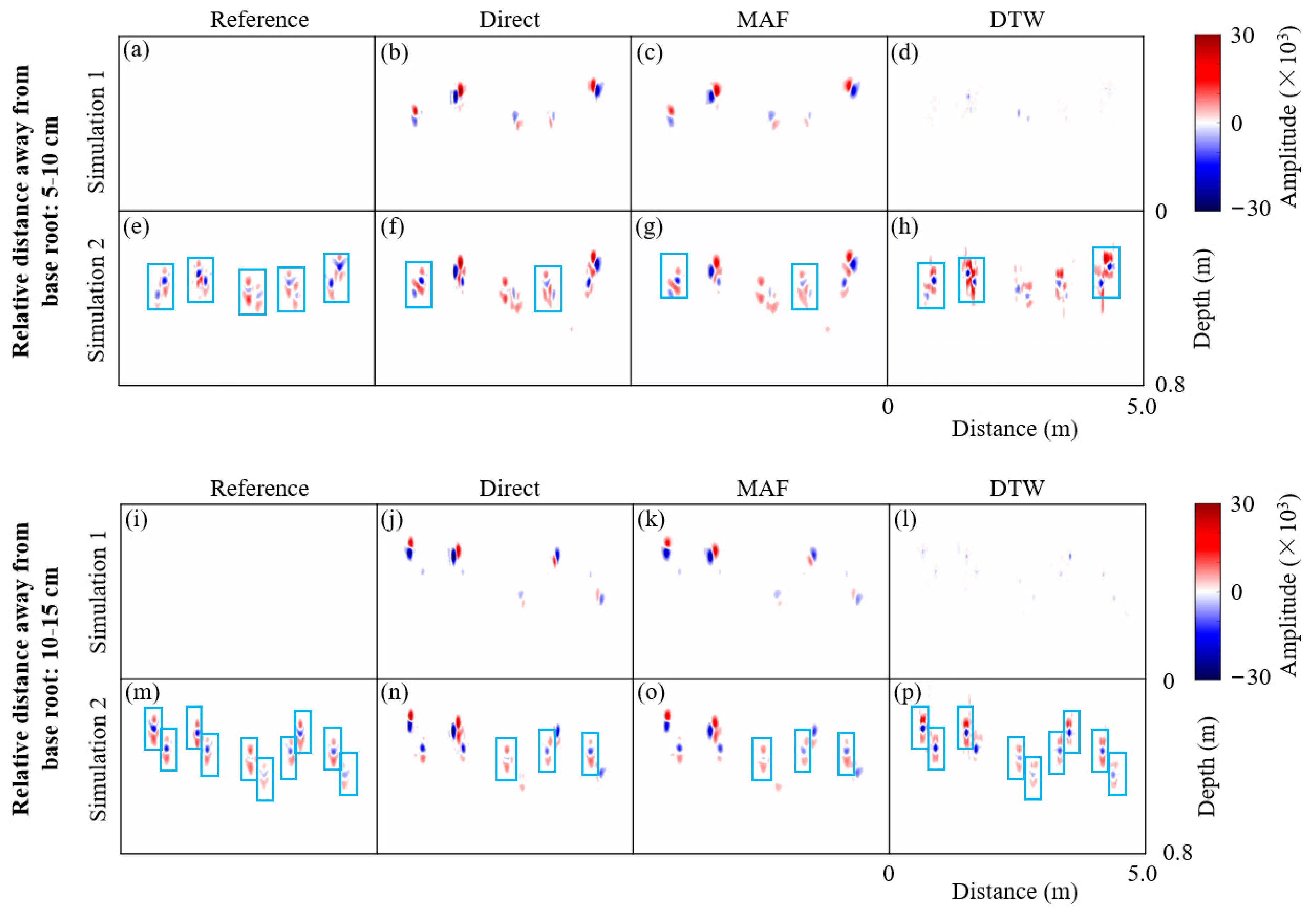
Figure 9 shows the differential result between the TL image and the background image after processing by various methods in the case of the coexistence of multiple root systems with diverse degrees of geometric offsets. Due to space limitations, only the results of the differences in the distance moved by the mobile root to the base root in the range of 0–5 cm and 15–20 cm are shown. Table 4 shows corresponding quantitative evaluation results. Additional details regarding the differences in the distance moved by the mobile root to the base root within the 5–10 cm and 10–15 cm ranges are portrayed in Figure A1, along with corresponding evaluation results showcased in Table A1.
In the scenario with a relative distance of 0–5 cm. For Simulation 1 (Figure 9a–d), both “Direct” and “MAF” produced significant signals, which are far from the “Reference”. This is a false signal due to the geometric mismatch problem. Conversely, in “DTW”, minimal significant signals are observed, closely resembling the “Reference”. For Simulation 2 (Figure 9e–h), only two red-blue-red alternating signals (solid blue boxes) are observed in both “Direct” and “MAF”. In contrast, “DTW” is able to observe that there are five red-blue-red alternating signals, mirroring the count exhibited in the “Reference”. In the quantitative evaluation of Simulation 1 results (shown in Table 4), the MAE decreased from 112 to 16, reflecting an 86% decrease, while the RMSE decreased from 972 to 304, indicating a 69% decrease. Meanwhile, in Simulation 2, the MAE dropped from 202 to 147, representing a 27% decrease, and the RMSE dropped from 1355 to 1124, reflecting a 17% decrease.
In the scenario with a relative distance of 15–20 cm. For Simulation 1 (Figure 9i–l), both “Direct” and “MAF” generate noticeable signals, albeit only three signals, which still differ from “Reference”. In contrast, no significant signals are observed in “DTW”, which is consistent with “Reference”. For Simulation 2 (Figure 9m–p), both “Direct” and “MAF”, only display three red-blue-red alternating signals, a discrepancy that diverges from the nine signals shown in the “Reference”. Conversely, “DTW” accurately depicts all the expected signals. The results of its quantitative evaluation show that, in Simulation 1, the MAE decreases from 124 to 12, indicating a 90% decrease, while the RMSE decreases from 893 to 174, marking an 81% decrease. At the same time, in Simulation 2, the MAE decreases from 226 to 157, reflecting a 31% decrease, while the RMSE decreases from 1379 to 787, representing a 43% decrease.
In summary, irrespective of the relative distance between the mobile root and the base root, the differential results, obtained subsequent to the TLIAM–DTW, consistently mirror the “Reference”. This consistency underscores TLIAM–DTW’s proficiency in nearly eradicating the influence of geometric mismatch issues on the interpretation of differential results in TL images. Furthermore, it is of interest to note that the geometric alignment of the TLIAM–DTW improves as the relative distance between the mobile root and the base root increases.
3.2. Performance of the TLIAM–DTW Method for Field-Collected TL GPR Data
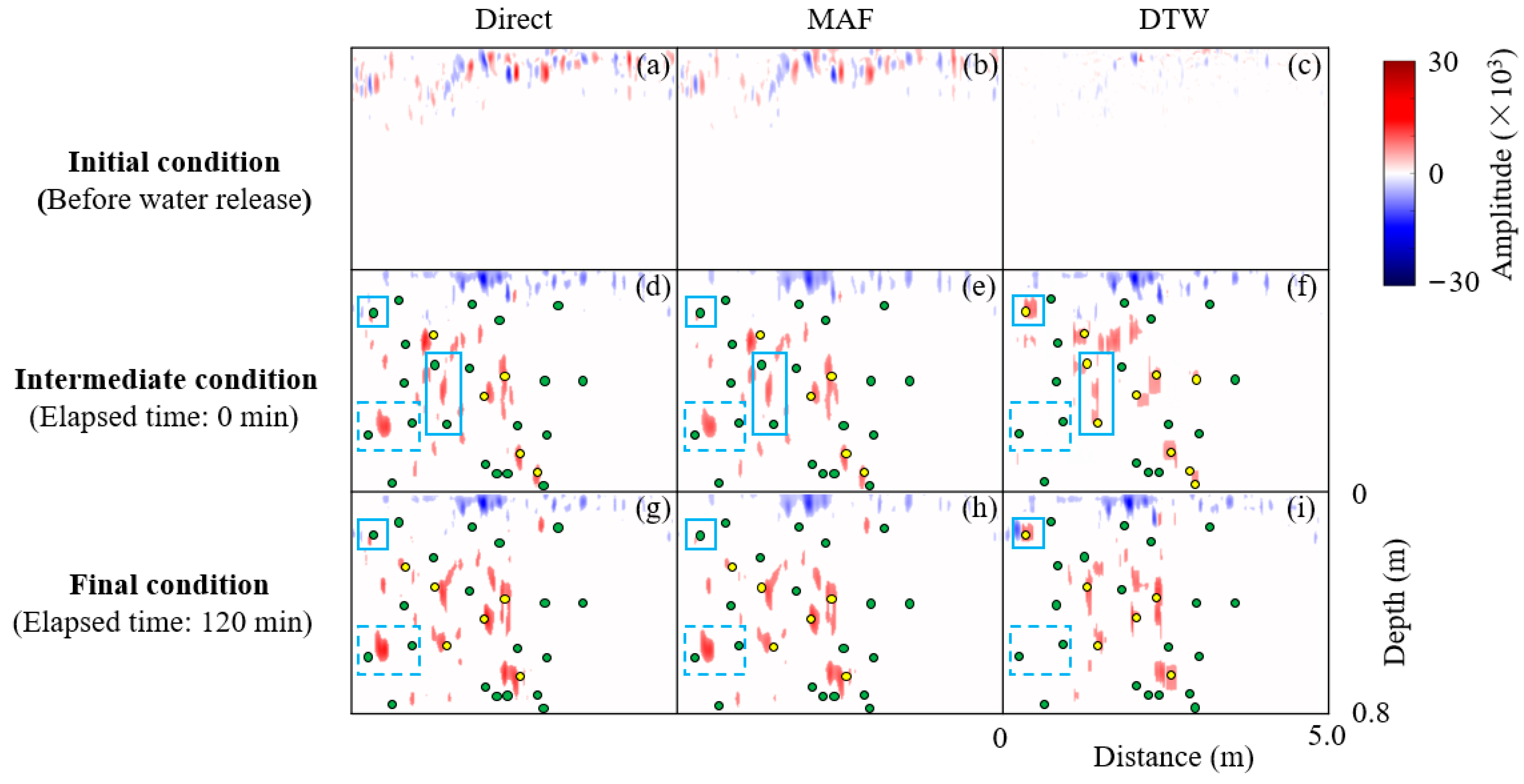
Figure 10 shows the differential results obtained after using various image alignment methods in the field measurement scenario. For the differential results of the two repetitive detections of the survey line before the infiltration experiments (Figure 10a–c), it can be seen that when “Direct” and “MAF” are compared, the signal in “DTW” is significantly reduced. The quantitative evaluation results in Table 5 corroborate the conclusions observed from the differential results. As there is no real image of the subsurface after the infiltration experiment, we only perform a quantitative evaluation of the geometric mismatch of the repeated soundings of the line before the infiltration experiments. The TLIAM–DTW, compared to the direct difference method, results in an 82% decrease in MAE, from 234 to 43, while the RMSE decreases from 1145 to 350, showing a decrease of 69%. At the end of the infiltration experiment (Figure 10d–i), a comparison the differential results of various alignment methods that considers the “DTW” shows that the matching relationship between the signal and the root system is improved. For example, in the blue solid line box, “Direct” and “MAF” exhibit signal disparities from the surrounding root system, whereas “DTW” portrays a more coherent match. Meanwhile, in the blue dashed box, there is an obvious and strong signal that disappeared after the TLIAM–DTW was used. And this signal did not form a match with the surrounding root system in “Direct” and “MAF”. This signal is therefore most likely a spurious signal, which is due to the geometric mismatch problem.
Therefore, TLIAM–DTW is effective in eliminating spurious signal variations caused by geometric mismatch while preserving the true differences caused by signal variations, both in forward simulation experiments and in field measurement experiments.
4. Discussion
4.1. The Influence of GPR Image Preprocessing on TLIAM–DTW Performance
The TLIAM–DTW method works with the A-scan signal, whose shape is influenced by the preprocessing steps applied to GPR data [43]. Taking “Lm5_Um5” in the simple single-root geometric mismatch scenarios as an example, differed results of image alignment methods are obtained after using the Kirchhoff migration (without using the Hilbert transform) during data preprocessing (Figure 11). Here, without the application of the Hilbert transform during preprocessing, Kirchhoff migration leads to distinct differences. Specifically, in simulation 1 (Figure 11a–d), comparing “Reference” with “DTW” reveals that the latter substantially rectifies geometric misalignments. However, additional arcs appear around the signal, an artifact arising from subjective decisions made during hyperbolic offset parameterization in the Kirchhoff migration [44]. If set improperly, these parameters can induce pronounced errors in the processed results, complicating the interpretation of these differences.
In simulation 2 (Figure 11e–h), although the signal variation after conducting TLIAM–DTW is more concentrated than that of direct subtraction between TL images, it still does not match the patterns shown in the reference image. Thus, preprocessing methods exert a significant impact on the quality of TL image alignment, as evidenced by the varying efficacies of the methods tested. The comparative analysis in Figure 7 and Figure 11 underscore the importance of the Hilbert transform in preprocessing in the optimization of TLIAM–DTW performance.
To address the issue discussed above, we propose a standard procedure for conducting the TLIAM–DTW method (Figure 12). It is important to acknowledge that the exact sequence of data preprocessing must be tailored to align with the unique attributes of the dataset at hand. Nonetheless, the overarching aim remains consistent (i.e., to eliminate extraneous clutter within the data and to enhance the signal-to-noise ratio of the GPR data). This optimization of data quality is pivotal for the successful application of the TLIAM–DTW method in achieving reliable and precise TL GPR image alignment.
4.2. Advantages and Limitations of the TLIAM–DTW Method
The geometric mismatch issue in TL-GPR images predominantly manifests as misalignments in A-scans, both horizontally, where corresponding A-scans fail to align properly, and vertically, through temporal shifts in A-scan waveforms caused by variations in subsurface permittivity during GPR surveys. Addressing this two-fold problem, the TLIAM–DTW method employs a dual strategy: horizontal matching and vertical warping. As delineated in studies [17,21], researchers have utilized the Pearson correlation coefficient to identify corresponding marker A-scans on the background image (i.e., pre-wetting condition) that match those in the subsequent TL image, with the aim of rectifying geometric mismatches in the horizontal plane. Table 6 shows the results of the Pearson correlation coefficient method versus the TLIAM–DTW method in pairing the marker A-scans in the background image corresponding to the A-scans in the TL image. Employing the DTW distance as a metric for horizontal matching substantially surpasses the accuracy of the Pearson correlation method (Table 6). This highlights the strength of the TLIAM–DTW method in aligning A-scans horizontally, hence providing a more precise solution to the geometric mismatch challenge in TL images.
To address the vertical aspect of the geometric mismatch problem, Biken and Versteeg [29] propose mitigating the time-shift anomaly in TL images by applying a uniform panning operation to the entire TL image. The amount of the overall panning of the TL image is based on the operator’s experience, introducing uncertainty to the results. However, actual signal variations within the TL image tend to be localized to specific zones, leading to the time shift of the A-scan waveform corresponding to these particular areas rather than the entire image. While uniform panning may rectify the temporal misalignment to an extent, it also runs the risk of injecting errors into segments where signal changes are not present, thereby potentially reducing the interpretative accuracy of the TL images. In contrast, the vertical warping process in the TLIAM–DTW method deploys a more nuanced approach for the vertical adjustment. It starts by ascertaining the presence of actual signal changes within the A-scans of the TL image. In the absence of actual signal variations, the A-scan is standardized using the DTW algorithm, thus aligning it in time without the influence of the operator’s subjective input. Whereas, if actual signal changes (such as those due to subsurface hydrological processes) are present, the adjustment is quantitatively affected, with the magnitude of the shift being carefully calculated based on the background soil’s relative permittivity and the central frequency of the GPR antenna. By accounting for these physical parameters, the TLIAM–DTW method strikes a balance between correcting for timeshifts and preserving the integrity of the true signal variations, thereby enhancing the fidelity and the interpretive quality of TL images.
Nonetheless, while the TLIAM–DTW method provides an innovative approach to solving geometric mismatch in TL GPR imaging, it is not without limitations. The first of these is an issue of overmatching, particularly when it comes to smaller geometric offsets (an example of this case can be observed in Figure 7h). In these instances, when horizontal offsets are ≤ 0.02 m, the method’s tendency to overmatch can cloud the interpretation of discrepancy signals, thereby challenging the formation of a precise quantitative link to the actual subsurface hydrological processes. Although overmatching does not compromise the detection of actual discrepancy signals, its effect on the subsequent analysis can possibly be considerable (e.g., the quantification of changes in soil moisture). The second limitation pertains to the method’s dependency on the distinctive recognition of different roots (or other point reflectors) within the subterranean environment. While TLIAM–DTW effectively eliminates errors stemming from geometric mismatches and preserves actual differential signals, the clarity with which it can distinguish between point reflectors is susceptible to several influencing factors, including the frequency of the utilized antenna and the survey direction [43,44], amongst others. Such factors can potentially change the differentiation between point reflectors, thereby constraining the TLIAM–DTW method’s efficacy in scenarios where distinct identification is crucial [42,44].
4.3. Future Outlooks
In the current study, the TLIAM method involves selecting marker A-scans based on a predetermined fixed spacing for horizontal matching. This rigid procedure could inadvertently overlook critical data within prominent regions of the image, such as areas with shape soil water changes. Such regions often hold significant interest in TL image studies, as they may encapsulate key aspects of the subsurface features or changes over time [20]. Acknowledging this potential shortfall, it is proposed that future research of TL image alignment should refine the horizontal matching step. Specifically, A-scans located in these emphasized regions should also be considered as marker A-scans. By incorporating these strategically important A-scans, the horizontal matching process would likely become more sensitive to the nuances of the TL images, which could greatly enhance the effectiveness of the alignment method by ensuring that vital spatial information is not disregarded, thereby improving the effectiveness of the resulting aligned TL images in capturing the dynamics under study
Following the removal of false signals stemming from the geometric mismatch in the differential results of TL images, the remaining authentic signals are correlated with the actual infiltration process. This correlation is instrumental in establishing a quantitative relationship between the signals and soil water content, facilitating the quantification of the impact of the infiltration process on soil water content.
The refinement of the TL-GPR method through the effective removal of spurious signals caused by geometric mismatch enhances the integrity of the differential results between TL images. Post-cleanup, the residual differential signals can be accurately correlated with the actual subsurface hydrological processes. Establishing this link is crucial, as it forms the basis for a quantitative relationship that connects the observed GPR signals to variations in soil water content. This quantitative insight is valuable for advancing our understanding of subsurface hydrological dynamics and improving the management of water resources in various applications.
During validation, the efficacy of the TLIAM–DTW method was assessed using gprMax V3.0 to create simulated TL GPR images. These simulations were conducted under idealized conditions with a uniform soil background, which enabled the minimization of clutter-related interference in the images. Root reflectors were also simplified, depicted as being distributed uniformly, both horizontally and at the same depth. This controlled setting facilitated the evaluation of the TLIAM–DTW method without the confounding variables present in real-world conditions. However, these ideal conditions notably differ from the complex and heterogeneous nature of actual soil environments where field applications take place. In reality, soil background can exhibit significant spatial heterogeneity, resulting in the presence of multiple clutter signals, thus, making the interpretation of GPR results more challenging [37,38]. Additionally, root distributions in nature do not follow a uniform pattern but are instead random and often entangled, giving rise to intricate hyperbolic signals that can overlap and affect one another, potentially causing incomplete or ambiguous signals within the GPR images [42,43]. Furthermore, the empirical validation of the TLIAM–DTW method has been limited to flat slope conditions within a forested area. This specific and somewhat uniform environment does not fully represent the myriad of surface conditions encountered in practical applications. Consequently, it is crucial to conduct extensive experimental validations under a broader range of complex surface and subsurface conditions. This additional testing is essential to confirm the method’s robustness and suitability for diverse field applications that involve more intricate soil and root system dynamics.
5. Conclusions
In conclusion, this study establishes the TLIAM–DTW method, an innovative TL GPR image alignment method that leverages the DTW algorithm to overcome the challenge of geometric misalignment in TL-GPR datasets. The robustness of the TLIAM–DTW method is thoroughly examined by using comprehensive simulated datasets and field-collected data. Both qualitative observations and quantitative analyses indicate that TLIAM–DTW outperforms the traditional TL-GPR alignment methods (e.g., moving average filtering) by effectively attenuating spurious signals attributable to geometric inconsistencies and preserving actual GPR signal variations that are associated with subsurface hydrological dynamics. The effectiveness of the TLIAM–DTW method is evident in its enhanced accuracy to delineate the dynamic features of subsurface lateral flow with greater reliably. This improvement captures the spatial and temporal intricacies inherent in subsurface hydrological processes, thereby advancing the precision of geophysical monitoring of subsurface hydrology under field conditions.
Author Contributions
Conceptualization, L.G. and J.W.; data curation, L.G., J.S. and J.W.; formal analysis, J.W., X.C. and L.G.; investigation, L.G., Y.J., T.H., X.L. and J.W.; methodology, J.W. and Y.Z.; software, J.W., X.L., J.S. and T.H.; visualization, J.W., Y.Z., X.C. and L.G.; writing—original draft, J.W.; writing—review and editing, all authors; funding acquisition, X.C. and L.G. All authors have read and agreed to the published version of the manuscript.
Funding
This research was funded by the National Key R & D Program of China (Grant 2023YFD1901203), the National Natural Science Foundation of China (Grant 42271329), and Sichuan Province Science and Technology Program (2022YFQ0066). Any opinions, findings, and conclusions or recommendations expressed in this material are those of the authors and do not necessarily reflect the views of the funding agencies.
Data Availability Statement
The source code of the TLIAM-DTW method and the dataset on GPR images are available from the authors upon request.
Conflicts of Interest
The authors declare no conflicts of interest.
Appendix A
Figure A1.
Examples of the differential results of various methods applied to the complex multiple-root geometric mismatch scenario. The solid blue box indicates a complete signal with red-blue-red alternation. (a,e,i,m) were the ideal differential result without the presence of geometric mismatch, denoted as “Reference”; (b,f,j,n) were the differential result without image alignment processing, denoted as “Direct”; (c,g,k,o) were the differential result with image alignment processing using moving average filter, denoted as “MAF”; (d,h,l,p) were the differential result with image alignment processing using the TLIAM–DTW, denoted as “DTW”.


Table A1.
Differential evaluation results obtained by various methods applied in complex multiple-root geometric mismatch scenarios.
Table A1.
Differential evaluation results obtained by various methods applied in complex multiple-root geometric mismatch scenarios.
| Relative Distance away from Base Root (cm) | Simulation Type | Method | MAE | RMSE |
|---|---|---|---|---|
| Direct | 145 | 1436 | ||
| Simulation 1 | MAF | 132 | 1200 | |
| 5–10 | TLIAM-DTW | 13 | 185 | |
| Direct | 210 | 1348 | ||
| Simulation 2 | MAF | 193 | 1156 | |
| TLIAM-DTW | 242 | 1378 | ||
| Direct | 130 | 1364 | ||
| Simulation 1 | MAF | 121 | 1138 | |
| 10–15 | TLIAM-DTW | 13 | 182 | |
| Direct | 204 | 1328 | ||
| Simulation 2 | MAF | 187 | 1134 | |
| TLIAM-DTW | 161 | 841 |
References
- Butnor, J.R.; Doolittle, J.; Kress, L.; Cohen, S.; Johnsen, K.H. Use of ground-penetrating radar to study tree roots in the southeastern United States. Tree Physiol. 2001, 21, 1269–1278. [Google Scholar] [CrossRef]
- Davis, J.L.; Annan, A.P. Ground-penetrating radar for high-resolution mapping of soil and rock stratigraphy. Geophys. Prospect. 1989, 37, 531–551. [Google Scholar] [CrossRef]
- Angermann, L.; Jackisch, C.; Allroggen, N.; Sprenger, M.; Zehe, E.; Tronicke, J.; Weiler, M.; Blume, T. Form and function in hillslope hydrology: Characterization of subsurface flow based on response observations. Hydrol. Earth Syst. Sci. 2017, 21, 3727–3748. [Google Scholar] [CrossRef]
- Jackisch, C.; Angermann, L.; Allroggen, N.; Sprenger, M.; Blume, T.; Tronicke, J.; Zehe, E. Form and function in hillslope hydrology: In situ imaging and characterization of flow-relevant structures. Hydrol. Earth Syst. Sci. 2017, 21, 3749–3775. [Google Scholar] [CrossRef]
- Hruska, J.; Čermák, J.; Šustek, S. Mapping tree root systems with ground-penetrating radar. Tree Physiol. 1999, 19, 125–130. [Google Scholar] [CrossRef]
- Kinlaw, A.; Grasmueck, M. Evidence for and geomorphologic consequences of a reptilian ecosystem engineer: The burrowing cascade initiated by the Gopher Tortoise. Geomorphology 2012, 157–158, 108–121. [Google Scholar] [CrossRef]
- Qiu, X.; Ding, C. Radar Observation of the Lava Tubes on the Moon and Mars. Remote Sens. 2023, 15, 2850. [Google Scholar] [CrossRef]
- Lantini, L.; Tosti, F.; Giannakis, I.; Zou, L.; Benedetto, A.; Alani, A.M. An Enhanced Data Processing Framework for Mapping Tree Root Systems Using Ground Penetrating Radar. Remote Sens. 2020, 12, 3417. [Google Scholar] [CrossRef]
- Doolittle, J.A.; Jenkinson, B.; Hopkins, D.; Ulmer, M.; Tuttle, W. Hydropedological investigations with ground-penetrating radar (GPR): Estimating water-table depths and local ground-water flow pattern in areas of coarse-textured soils. Geoderma 2006, 131, 317–329. [Google Scholar] [CrossRef]
- Doolittle, J.; Zhu, Q.; Zhang, J.; Guo, L.; Lin, H. Geophysical investigations of soil-landscape architecture and its impacts on subsurface flow. In Hydropedology: Synergistic Integration of Soil Science and Hydrology; Academic Press: Cambridge, MA, USA; Elsevier: Amsterdam, The Netherlands, 2012; pp. 413–447. [Google Scholar]
- Jia, S.; Zhang, T.; Hao, J.; Li, C.; Michaelides, R.; Shao, W.; Wei, S.; Wang, K.; Fan, C. Spatial Variability of Active Layer Thickness along the Qinghai–Tibet Engineering Corridor Resolved Using Ground-Penetrating Radar. Remote Sens. 2022, 14, 5606. [Google Scholar] [CrossRef]
- Luo, Z.; Niu, J.; Xie, B.; Zhang, L.; Chen, X.; Berndtsson, R.; Du, J.; Ao, J.; Yang, L.; Zhu, S. Influence of Root Distribution on Preferential Flow in Deciduous and Coniferous Forest Soils. Forests 2019, 10, 986. [Google Scholar] [CrossRef]
- Butnor, J.R.; Doolittle, J.; Johnsen, K.H.; Samuelson, L.; Stokes, T.; Kress, L. Utility of ground-penetrating radar as a root biomass survey tool in forest systems. Soil Sci. Soc. Am. J. 2003, 67, 1607–1615. [Google Scholar] [CrossRef]
- Barton, C.V.; Montagu, K.D. Detection of tree roots and determination of root diameters by ground penetrating radar under optimal conditions. Tree Physiol. 2004, 24, 1323–1331. [Google Scholar] [CrossRef]
- Topp, G.C.; Davis, J.; Annan, A.P. Electromagnetic determination of soil water content: Measurements in coaxial transmission lines. Water Resour. Res. 1980, 16, 574–582. [Google Scholar] [CrossRef]
- Guo, L.; Chen, J.; Lin, H. Subsurface lateral preferential flow network revealed by time-lapse ground-penetrating radar in a hillslope. Water Resour. Res. 2014, 50, 9127–9147. [Google Scholar] [CrossRef]
- Trinks, I.; Stümpel, H.; Wachsmuth, D. Monitoring water flow in the unsaturated zone using georadar. First Break. 2001, 19, 12. [Google Scholar]
- Haarder, E.B.; Looms, M.C.; Jensen, K.H.; Nielsen, L. Visualizing Unsaturated Flow Phenomena Using High-Resolution Reflection Ground Penetrating Radar. Vadose Zone J. 2011, 10, 84–97. [Google Scholar] [CrossRef]
- Robinson, J.; Buda, A.; Collick, A.; Shober, A.; Ntarlagiannis, D.; Bryant, R.; Slater, L. Electrical monitoring of saline tracers to reveal subsurface flow pathways in a flat ditch-drained field. J. Hydrol. 2020, 586, 124862. [Google Scholar] [CrossRef]
- Nyquist, J.E.; Toran, L.; Pitman, L.; Guo, L.; Lin, H. Testing the Fill-and-Spill Model of Subsurface Lateral Flow Using Ground-Penetrating Radar and Dye Tracing. Vadose Zone J. 2018, 17, 1–13. [Google Scholar] [CrossRef]
- Di Prima, S.; Winiarski, T.; Angulo-Jaramillo, R.; Stewart, R.D.; Castellini, M.; Abou Najm, M.R.; Ventrella, D.; Pirastru, M.; Giadrossich, F.; Capello, G.; et al. Detecting infiltrated water and preferential flow pathways through time-lapse ground-penetrating radar surveys. Sci. Total Environ. 2020, 726, 138511. [Google Scholar] [CrossRef] [PubMed]
- Di Prima, S.; Giannini, V.; Ribeiro Roder, L.; Giadrossich, F.; Lassabatere, L.; Stewart, R.D.; Abou Najm, M.R.; Longo, V.; Campus, S.; Winiarski, T.; et al. Coupling time-lapse ground penetrating radar surveys and infiltration experiments to characterize two types of non-uniform flow. Sci. Total Environ. 2022, 806, 150410. [Google Scholar] [CrossRef] [PubMed]
- Truss, S.; Grasmueck, M.; Vega, S.; Viggiano, D.A. Imaging rainfall drainage within the Miami oolitic limestone using high-resolution time-lapse ground-penetrating radar. Water Resour. Res. 2007, 43, 3. [Google Scholar] [CrossRef]
- Deiana, R.; Cassiani, G.; Villa, A.; Bagliani, A.; Bruno, V. Calibration of a Vadose Zone Model Using Water Injection Monitored by GPR and Electrical Resistance Tomography. Vadose Zone J. 2008, 7, 215–226. [Google Scholar] [CrossRef]
- Steelman, C.M.; Endres, A.L.; Jones, J.P. High-resolution ground-penetrating radar monitoring of soil moisture dynamics: Field results, interpretation, and comparison with unsaturated flow model. Water Resour. Res. 2012, 48, 9. [Google Scholar] [CrossRef]
- Koyama, C.N.; Liu, H.; Takahashi, K.; Shimada, M.; Watanabe, M.; Khuut, T.; Sato, M. In-Situ Measurement of Soil Permittivity at Various Depths for the Calibration and Validation of Low-Frequency SAR Soil Moisture Models by Using GPR. Remote Sens. 2017, 9, 580. [Google Scholar] [CrossRef]
- Allroggen, N.; van Schaik, N.L.M.B.; Tronicke, J. 4D ground-penetrating radar during a plot scale dye tracer experiment. J. Appl. Geophys. 2015, 118, 139–144. [Google Scholar] [CrossRef]
- Mangel, A.R.; Moysey, S.M.J.; Bradford, J. Reflection tomography of time-lapse GPR data for studying dynamic unsaturated flow phenomena. Hydrol. Earth Syst. Sci. 2020, 24, 159–167. [Google Scholar] [CrossRef]
- Birken, R.; Versteeg, R. Use of four-dimensional ground penetrating radar and advanced visualization methods to determine subsurface fluid migration. J. Appl. Geophys. 2000, 43, 215–226. [Google Scholar] [CrossRef]
- Ge, L.; Chen, S. Exact dynamic time warping calculation for weak sparse time series. Appl. Soft Comput. 2020, 96, 106631. [Google Scholar] [CrossRef]
- Maus, V.; Câmara, G.; Cartaxo, R.; Sanchez, A.; Ramos, F.M.; De Queiroz, G.R. A time-weighted dynamic time warping method for land-use and land-cover mapping. IEEE J-STARS 2016, 9, 3729–3739. [Google Scholar] [CrossRef]
- Lin, H. Temporal stability of soil moisture spatial pattern and subsurface preferential flow pathways in the Shale Hills Catchment. Vadose Zone J. 2006, 5, 317–340. [Google Scholar] [CrossRef]
- Lin, H.; Zhou, X. Evidence of subsurface preferential flow using soil hydrologic monitoring in the Shale Hills catchment. Eur. J. Soil Sci. 2007, 59, 34–49. [Google Scholar] [CrossRef]
- Liu, H.; Lin, H. Frequency and Control of Subsurface Preferential Flow: From Pedon to Catchment Scales. Soil Sci. Soc. Am. J. 2015, 79, 362–377. [Google Scholar] [CrossRef]
- Giannakis, I. Realistic Numerical Modelling of Ground Penetrating Radar for Landmine Detection; University of Edinburgh: Edinburgh, UK, 2016. [Google Scholar]
- Arrow, K.J.; Hurwicz, L. Competitive stability under weak gross substitutability: The “Euclidean distance” approach. Int. Econ. Rev. 1960, 1, 38–49. [Google Scholar] [CrossRef]
- Itakura, F. Minimum prediction residual principle applied to speech recognition. IEEE Trans. Acoust. Speech Signal Process. 1975, 23, 67–72. [Google Scholar] [CrossRef]
- Hale, D. Dynamic warping of seismic images. Geophysics 2013, 78, S105–S115. [Google Scholar] [CrossRef]
- Guo, L.; Mount, G.J.; Hudson, S.; Lin, H.; Levia, D. Pairing geophysical techniques improves understanding of the near-surface Critical Zone: Visualization of preferential routing of stemflow along coarse roots. Geoderma 2020, 357, 113953. [Google Scholar] [CrossRef]
- Zhang, J.; Lin, H.; Doolittle, J. Soil layering and preferential flow impacts on seasonal changes of GPR signals in two contrasting soils. Geoderma 2014, 213, 560–569. [Google Scholar] [CrossRef]
- Guo, L.; Lin, H.; Fan, B.; Cui, X.; Chen, J. Forward simulation of root’s ground penetrating radar signal: Simulator development and validation. Plant Soil 2013, 372, 487–505. [Google Scholar] [CrossRef]
- Holden, J. Hydrological connectivity of soil pipes determined by ground-penetrating radar tracer detection. Earth Surf. Process. Landforms. 2004, 29, 437–442. [Google Scholar] [CrossRef]
- Guo, L.; Chen, J.; Cui, X.; Fan, B.; Lin, H. Application of ground penetrating radar for coarse root detection and quantification: A review. Plant Soil 2012, 362, 1–23. [Google Scholar] [CrossRef]
- Butnor, J.R.; Samuelson, L.J.; Stokes, T.A.; Johnsen, K.H.; Anderson, P.H.; González-Benecke, C.A. Surface-based GPR underestimates below-stump root biomass. Plant Soil. 2016, 402, 47–62. [Google Scholar] [CrossRef]
Figure 1.
Measuring the similarity between two time series (representing A-scan signals in TL-GPR images) by (a) the Euclidean distance; and (b) the DTW distance. (c) The DTW algorithm searches for the optimal path of two time series to ensure the least distance from the starting point to the ending point. R and T represented two time series with lengths of m and n, respectively. indicated the minimal warping path.

Figure 2.
TL-GPR image alignment procedure. The red line represents the marker A-scans (i.e., marker traces), the green line represents the non-marker A-scans between the marker A-scans, and the blue line represents the non-marker A-scans at the beginning and end of a survey transect. (a) and (b) are the background image (as background) and TL image (as TL), respectively; (c) Using the DTW algorithm, the marker and non-marker A-scans are matched successively to solve the problem of inconsistent counts and mis-corresponding A-scans. For example, if the marker A-scan in the Background corresponds to in the TL image, is replaced by . The resulting new image is called TL1; (d) The time offset problem is solved by using the DTW algorithm to warp or overall translation the corresponding A-scans in TL using the A-scans in Background as the standard. The new image obtained was called TL2. At this point, the TL image alignment process is completed.

Figure 3.
Simple single-root geometric mismatch scenario forward modeling setting—only all possible offsets for a single root with a geometric offset distance of 0.01 m are shown. (a) The initial situation; (b–d) All possible offset scenarios that might occur for a single root with a geometric offset distance of 0.01 m in Simulation 1 (solely geometric mismatch); (e) The ideal situation after the occurrence of subsurface lateral flow; (f–h) All possible offset scenarios that could occur after the occurrence of subsurface lateral flow with a geometric offset distance of 0.01 m in Simulation 2 (which entails both geometric mismatch and real signal variations).

Figure 4.
Complex multiple-root geometric mismatch scenario forward modeling setting. There are five base roots and five mobile roots in the scenario. H represents the movement in the horizontal direction, and V represents the movement in the vertical direction.
Figure 4.
Complex multiple-root geometric mismatch scenario forward modeling setting. There are five base roots and five mobile roots in the scenario. H represents the movement in the horizontal direction, and V represents the movement in the vertical direction.

Figure 5.
(a) An overview of the Fair Hill Catchment, showing drainage boundaries (indicated by the yellow dashed lines) and the location of the sample tree; (b) Water was released onto the tree trunk through PVC tubing to represent the stemflow process; (c) A photo of the geophysical survey area, showing the antenna of the GPR system (the white box) and its moving path (indicated by the red solid line).

Figure 6.
An example of GPR data preprocessing effect: (a) Raw data from the forward simulation results of Figure 3a obtained by gprMax V3.0 (the settings are described in Section 2.2.1 above) and the hyperbolic reflections representing the root reflectors; (b) Some radargram processed in Reflexw 9.5 software with first arrival time extraction and background noise removal were used to improve the signal-to-noise ratio. The velocity analysis was then performed and the time–depth conversion was completed; (c) Kirchoff migration was used to trace hyperbola reflections back to their sources; (d) Hilbert transformation was used to express the magnitude of signals, elucidate subtle objects and reduce multiple reflections; (e) Moving average filter was used to eliminate the influence of geometric mismatch; (f) A graph of the A-scan obtained after the Hilbert transformation—at this point, only the amplitude values symbolizing the signal strength could be represented.

Figure 7.
Examples of the differential results from various methods applied to simple single-root geometric mismatch scenarios (“Lm1_Um1”, which represents the root offset 0.01 m to the left and 0.01 m upwards; and “Lm5_Um5”, similarly). (a,e,i,m) are the ideal differential result without the presence of geometric mismatch, denoted as “Reference”; (b,f,j,n) are the differential result without image alignment processing, denoted as “Direct”; (c,g,k,o) are the differential result with image alignment processing using the moving average filter, denoted as “MAF”; (d,h,l,p) are the differential result with image alignment processing using the TLIAM–DTW, denoted as “DTW”.

Figure 8.
Evaluation plot of differential results for single-root geometric mismatch scenarios. The number represents the median of the box. (a) is Simulation 1, where only geometric mismatch exists; (b) is Simulation 2, where true signal variations exist.
Figure 8.
Evaluation plot of differential results for single-root geometric mismatch scenarios. The number represents the median of the box. (a) is Simulation 1, where only geometric mismatch exists; (b) is Simulation 2, where true signal variations exist.

Figure 9.
Examples of the differential results of various methods applied to complex multiple-root geometric mismatch scenarios. The solid blue box indicates a complete signal with red-blue-red alternation. (a,e,i,m) are the ideal differential result without the presence of geometric mismatch, denoted as “Reference”; (b,f,j,n) are the differential result without image alignment processing, denoted as “Direct”; (c,g,k,o) are the differential result with image alignment processing using the moving average filter, denoted as “MAF”; (d,h,l,p) are the differential result with image alignment processing using the TLIAM–DTW, denoted as “DTW”.

Figure 10.
Comparison of differential results for the field measurement scenario. (a–c) represents the TL image alignment results before the infiltration experiment. (d–f,g–i) represent the TL image alignment results at 0 min and 120 min after the end of the infiltration experiment, respectively. (a,d,g) are the differential result without image alignment processing, denoted as “Direct”; (b,e,h) are the differential result with image alignment processing obtained using the moving average filter, denoted as “MAF”; (c,f,i) are the differential result with image alignment processing obtained using the TLIAM–DTW, denoted as “DTW”. The yellow dots in (d–i) refer to the lateral roots that are overlap with the isolated wetting areas (i.e., identifying the preferential flow pathways), evidencing the lateral root-derived preferential flow. The green dots in (d–i) indicate the lateral roots that do not contribute to preferential channelization. In (d–i), the solid blue boxes represent signals that are well-matched to the root system, while the dashed blue boxes indicate signals affected by geometric mismatch, which fail to connect with the root system.

Figure 11.
Differential results of TL images without Hilbert transform, after different alignment methods, using “Lm5_Um5” (refers to a leftward shift of 0.05 m and an upward shift of 0.05 m for root) in simple single-root geometric mismatch scenarios as an example. (a–h) the differential result of Simulation 1 and Simulation 2. (a,e) are the ideal differential result without the presence of geometric mismatch, denoted as “Reference”; (b,f) are the differential result without image alignment processing, denoted as “Direct”; (c,g) are the differential result with image alignment processing using the moving average filter, denoted as “MAF”; (d,h) are the differential result with image alignment processing using the TLIAM–DTW, denoted as “DTW”.

Figure 12.
The proposed standard procedure for conducting the TLIAM–DTW method.

Table 1.
Medium parameters setting.
| Medium | Water Content 1 | Relative Dielectric Constant | Static Conductivity (S·m−1) |
|---|---|---|---|
| Root (diameter = 0.02 m) | 90% | 13.08 | 0 |
| Background soil | 6% | 4.12 | 0.01 |
| Saturated soil 2 | 44% | 44.60 | 0.64 |
1 Volumetric water content for the soil, and the weight water content for the root. 2 Saturated soil refers to the soil completely infiltrated by water flow when subsurface lateral flow occurs.
Table 2.
Relative distance that the mobile root is away from the base root in a multi-root geometric mismatch scenario.
Table 2.
Relative distance that the mobile root is away from the base root in a multi-root geometric mismatch scenario.
| Variables 1 | Relative Distance away from Base Root (cm) | |||
|---|---|---|---|---|
| 0–5 | 5–10 | 10–15 | 15–20 | |
| H1 | −5 | −8 | −14 | −16 |
| V1 | +1 | −9 | 13 | −18 |
| H2 | −3 | −7 | −11 | −17 |
| V2 | 0 | 6 | 11 | 16 |
| H3 | 3 | 9 | 14 | 17 |
| V3 | 3 | −6 | −12 | 17 |
| H4 | 2 | 10 | 12 | 18 |
| V4 | 4 | −6 | 11 | −16 |
| H5 | 5 | 10 | 13 | 20 |
| V5 | −4 | 10 | −15 | 19 |
1 H represents the movement in the horizontal direction, + represents a right shift, − represents a left shift; V represents the movement in the vertical direction, + represents an upward shift, − represents a downward shift.
Table 3.
Geometric offset distance of mobile root in a multi-root geometric mismatch scenario.
| Offset Type | Geometric Offset Distance (cm) | ||||
|---|---|---|---|---|---|
| 1 | 2 | 3 | 4 | 5 | |
| Horizontal offset 1 | +1 | +5 | +3 | −2 | −4 |
| Vertical offset 2 | +4 | +3 | −3 | −2 | +2 |
1 + represents a right shift, − represents a left shift. 2 + represents an upward shift, − represents a downward shift.
Table 4.
Differential evaluation results obtained from the application of various methods in complex multiple-root geometric mismatch scenarios.
Table 4.
Differential evaluation results obtained from the application of various methods in complex multiple-root geometric mismatch scenarios.
| Relative Distance away from Base Root (cm) | Simulation Type | Method | MAE | RMSE |
|---|---|---|---|---|
| Direct | 112 | 972 | ||
| Simulation 1 | MAF | 103 | 828 | |
| 0–5 | TLIAM-DTW | 16 | 304 | |
| Direct | 202 | 1355 | ||
| Simulation 2 | MAF | 195 | 1235 | |
| TLIAM-DTW | 147 | 1124 | ||
| Direct | 124 | 893 | ||
| Simulation 1 | MAF | 115 | 1033 | |
| 15–20 | TLIAM-DTW | 12 | 174 | |
| Direct | 226 | 1379 | ||
| Simulation 2 | MAF | 216 | 1225 | |
| TLIAM-DTW | 157 | 787 |
Table 5.
Differential evaluation results of field scenario (Before water release).
| Method | MAE | RMSE |
|---|---|---|
| Direct | 234 | 1145 |
| MAF | 215 | 1018 |
| TLIAM-DTW | 43 | 350 |
Table 6.
Marker A-scans matching results for different methods, using “Lm5_Um5” in simple single-root geometric mismatch scenarios as an example.
Table 6.
Marker A-scans matching results for different methods, using “Lm5_Um5” in simple single-root geometric mismatch scenarios as an example.
| Number of Marker A-Scan in the Background Image | Number of Corresponding A-Scan in the TL Image | Simulation 1 | Simulation 2 | ||
|---|---|---|---|---|---|
| Different Methods | Different Methods | ||||
| Pearson Correlation Coefficient | DTW Distance | Pearson Correlation Coefficient | DTW Distance | ||
| 10 | 10 | 10 | 10 | 10 | 10 |
| 20 | 20 | 20 | 20 | 20 | 20 |
| 30 | 30 | 30 | 30 | 30 | 30 |
| 40 | 40 | 40 | 40 | 40 | 40 |
| 50 | 55 | 53 | 55 | 51 | 55 |
| 60 | 65 | 64 | 65 | 62 | 65 |
| 70 | 75 | 74 | 75 | 73 | 75 |
| 80 | 85 | 84 | 85 | 83 | 85 |
| 90 | 95 | 94 | 95 | 93 | 95 |
Disclaimer/Publisher’s Note: The statements, opinions and data contained in all publications are solely those of the individual author(s) and contributor(s) and not of MDPI and/or the editor(s). MDPI and/or the editor(s) disclaim responsibility for any injury to people or property resulting from any ideas, methods, instructions or products referred to in the content. |
© 2024 by the authors. Licensee MDPI, Basel, Switzerland. This article is an open access article distributed under the terms and conditions of the Creative Commons Attribution (CC BY) license (https://creativecommons.org/licenses/by/4.0/).
Share and Cite
MDPI and ACS Style
Wen, J.; Huang, T.; Cui, X.; Zhang, Y.; Shi, J.; Jiang, Y.; Li, X.; Guo, L. Enhancing Image Alignment in Time-Lapse-Ground-Penetrating Radar through Dynamic Time Warping. Remote Sens. 2024, 16, 1040. https://doi.org/10.3390/rs16061040
AMA Style
Wen J, Huang T, Cui X, Zhang Y, Shi J, Jiang Y, Li X, Guo L. Enhancing Image Alignment in Time-Lapse-Ground-Penetrating Radar through Dynamic Time Warping. Remote Sensing. 2024; 16(6):1040. https://doi.org/10.3390/rs16061040
Chicago/Turabian StyleWen, Jiahao, Tianbao Huang, Xihong Cui, Yaling Zhang, Jinfeng Shi, Yanjia Jiang, Xiangjie Li, and Li Guo. 2024. "Enhancing Image Alignment in Time-Lapse-Ground-Penetrating Radar through Dynamic Time Warping" Remote Sensing 16, no. 6: 1040. https://doi.org/10.3390/rs16061040
Note that from the first issue of 2016, this journal uses article numbers instead of page numbers. See further details here.