An Ensemble-Based Framework for Sophisticated Crop Classification Exploiting Google Earth Engine

Abstract

Corn and soybeans play pivotal roles in the agricultural landscape of the United States, and accurately delineating their cultivation areas is indispensable for ensuring food security and addressing hunger-related challenges. Traditional methods for crop mapping are both labor-intensive and time-consuming. Fortunately, the advent of high-resolution imagery, exemplified by Sentinel-2A (S2A), has opened avenues for precise identification of these crops at a field scale, with the added advantage of cloud computing. This paper presents an innovative algorithm designed for large-scale mapping of corn and soybean planting areas on the Google Cloud Engine, drawing inspiration from symmetrical theory. The proposed methodology encompasses several sequential steps. First, S2A data undergo processing incorporating phenological information and spectral characteristics. Subsequently, texture features derived from the grayscale matrix are synergistically integrated with spectral features in the first step. To enhance algorithmic efficiency, the third step involves a feature importance analysis, facilitating the retention of influential bands while eliminating redundant features. The ensuing phase employs three base classifiers for feature training, and the final result maps are generated through a collective voting mechanism based on the classification results from the three classifiers. Validation of the proposed algorithm was conducted in two distinct research areas: Ford in Illinois and White in Indiana, showcasing its commendable classification capabilities for these crops. The experiments underscore the potential of this method for large-scale mapping of crop areas through the integration of cloud computing and high-resolution imagery.

1. Introduction

In the intricate tapestry of global agriculture, the precise identification and monitoring of crop cultivation areas have become paramount for sustaining food security [1] and addressing the ever-growing challenges of a burgeoning world population [2]. Traditional field surveys offer the advantage of direct observation, facilitating detailed assessments of crop health, growth stages, and yield estimation. However, they are limited by being time-consuming, labor-intensive, and less scalable. Moreover, field surveys may not capture large-scale or inaccessible areas, presenting challenges in comprehensive monitoring [3]. Enter the realm of remote sensing, an indispensable technological frontier that offers unprecedented insights into agricultural landscapes [4]. In this context, the fusion of cutting-edge remote-sensing techniques with advanced computational tools emerges as a crucial paradigm, with the potential not only to revolutionize our understanding of crop dynamics but also to empower decision-makers in devising resilient and sustainable agricultural strategies [5].

With the launch of the Sentinel mission, remote sensing has become more capable of providing higher-quality multispectral data. Hyperspectral and multispectral datasets have been studied extensively in recent decades to monitor crops [6]. Numerous studies have utilized remote-sensing techniques to estimate crop areas based on large agricultural areas and complex measurements [7,8]. To monitor large-scale crops, however, a significant number of orbital images must be processed, which requires complex computing infrastructure to manage, process, and store the data. Classifying and processing remote-sensing images using machine learning is an effective method. These algorithms can identify patterns in the multispectral data and classify different types of crops, allowing for precise measurements of crop yields and monitoring of agricultural conditions [9]. Moreover, machine learning techniques can help automate the detection of anomalies, such as pest infestations, nutrient deficiencies, and water stress, enabling farmers to take proactive measures to prevent yield losses [10]. With the rapid advancement of machine learning and remote-sensing technology, it is anticipated that precision agriculture will become more widely adopted, providing farmers with a more effective means of managing their crops and increasing their overall productivity.

Presently, the use of various open-source software has greatly promoted the development of image processing. Python and R [11] are two effective programming languages for image processing. Since 2010, Google has provided the free cloud computing and computing platform known as the Google Earth Engine (GEE) [12]. This platform offers access to various open-source spatial datasets, such as Sentinel, Landsat, MODIS, and the Global Forest Change dataset. In addition, it has petabytes of geospatial data [13]. Python and JavaScript APIs are also available to analyze these data efficiently. The entire GEE data catalog is stored in Google’s Data Center, which is equipped with high-performance CPUs that allow for complex analysis calculations. The platform’s powerful computing capabilities enable the implementation of proposed algorithms, with JavaScript being the primary language used in system implementation.

In recent years, many scholars have used the rich data on the GEE platform to conduct experimental research [14]. For example, researchers have used GEE to analyze changes in land cover [15], monitor deforestation [16], and predict crop yields [17]. The platform’s ability to quickly and efficiently process large amounts of data has made it a valuable tool for environmental and agricultural research. Additionally, GEE has been used for disaster response and management [18], as it allows for real-time monitoring of natural disasters and other emergencies. Overall, the Google Earth Engine has revolutionized the way people access and analyze geospatial data, opening up new possibilities for research and innovation in fields ranging from climate science to urban planning. Therefore, we implemented a novel decision ensemble-based method for the classification of corn and soybean based on GEE (corn and soybean classification algorithm, abbreviated as CSA).

The main contributions of this work are:

• The proposed algorithm ensembles both spatial and spectral features to improve the accuracy of crop mapping. It allows the algorithm to capture the spatial and spectral variations of the crops, resulting in more accurate classification results.
• A novel approach that involves combining the decisions of three supervised classifiers is utilized. The algorithm uses the collective intelligence of three classifiers to improve the accuracy and robustness of the classification, as well as reduce the bias introduced using a single classifier.
• The proposed algorithm, implemented on the Google Earth Engine (GEE) platform, capitalizes on its efficient processing of large-scale satellite imagery data. Leveraging the distributed computing capabilities of GEE enables swift and effective processing of extensive datasets, resulting in considerable time savings. Compared to traditional labor-intensive and time-consuming crop mapping methods, this approach harnesses high-resolution imagery and cloud computing resources to offer a more efficient and precise means of identifying corn and soybean cultivation areas at a field scale. Such advancements have the potential to streamline agricultural monitoring and management processes, ultimately saving valuable time and resources.

The major parts of this paper are divided as follows. Section 2 introduces the relevant algorithms of supervised learning used in this paper. Section 3 describes the proposed methodology in detail. Section 4 shows the results of the experiments. Section 5 conducts an in-depth analysis of the proposed algorithm in conjunction with the observational data obtained from the validation dataset. Section 6 draws the conclusion.

2. Classifying Algorithms

2.1. Random Forest (RF)

The random forest algorithm combines multiple decision trees, and each training set is randomly back-selected while randomly selecting some features as input, and finally using the idea of bagging to integrate the results [19,20]. Bagging assumes that there is a training dataset of size N, and each time there is a sub-dataset of size M selected from the dataset, a total of K times are selected, and K models are trained and learned according to these K sub-datasets [21]. Therefore, the random forest algorithm can be regarded as a bagging algorithm with decision trees as estimators.

2.2. Classification and Regression Tree (CART)

The learning of the decision tree is essential to summarize a set of classification rules from the training dataset so that it has less contradiction with the training data [22]. When faced with data with multiple attributes, the practice of the decision tree is to select one attribute at a time to judge, and if it cannot be concluded, continue to select other attributes to judge until the result can be judged “with certainty” or the above attributes have been used. CART is a criterion for categorical regression trees that use the Gini index as a criterion for selecting features [23].

2.3. Support Vector Machine (SVM)

SVM is a dichotomous model, and its basic model is a linear classifier with the largest interval defined on the feature space, which distinguishes it from the perceptron [24]. SVM also includes kernel tricks, which makes it essentially a nonlinear classifier. The learning strategy of SVM is interval maximization, which can be formalized as a problem-solving convex quadratic programming, which is also equivalent to the problem of minimizing the loss function of the regularized hinge.

3. Proposed Method

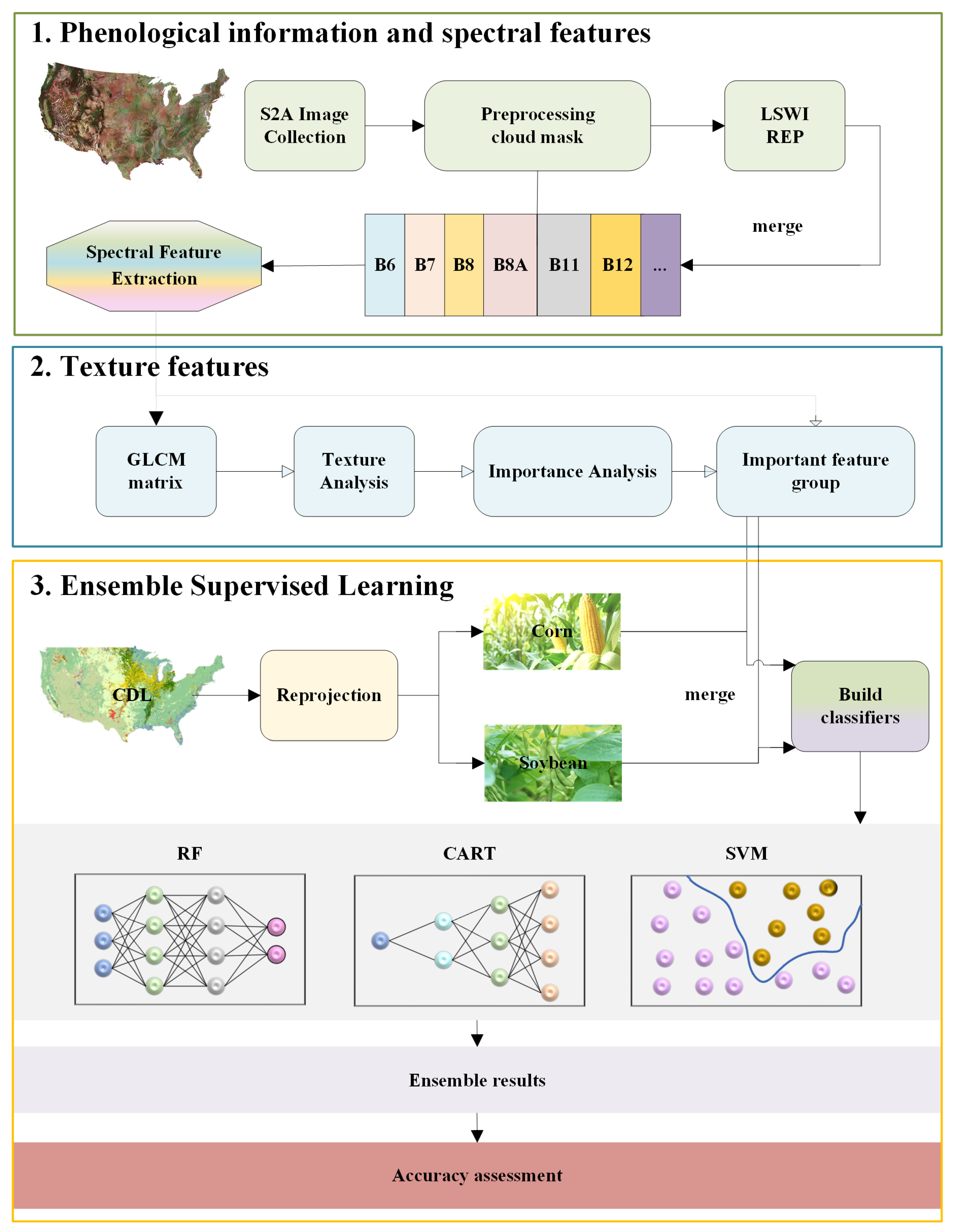
In this paper, we present an algorithm that allows for the efficient mapping of corn and soybean planting areas on Google Cloud Engine. The proposed method involves several distinct steps that are designed to maximize accuracy and efficiency. Specifically, the algorithm leverages phenological information and spectral characteristics to process Sentinel-2A (S2A) data in the first step. In the second step, texture features are obtained from grayscale matrices and are combined with spectral features in an ensemble fashion. Feature importance analysis is then used to retain only the most influential bands, which improves the overall efficiency of the algorithm. The fourth step involves the use of three classifiers as base classifiers to train the features, and the final step involves collective voting on three classification results to obtain accurate and reliable result maps. To clearly illustrate the algorithm flow, the overall description of the CSA is shown in Figure 1.

3.1. Preprocessing

To achieve accurate land crop classification, it is crucial to establish a reliable primary dataset. Clouds and fog can significantly impact datasets, so a key preprocessing step involves creating a cloud mask to mitigate these effects. Hence, it is prioritized de-clouding the data to enhance dataset quality and reduce interference. Specifically, the ‘QA60’ band is selected, and the Opaque clouds and Cirrus clouds are set to 0 to generate a cloud mask.

3.2. Phenological Information and Spectral Features

3.2.1. Phenological Information

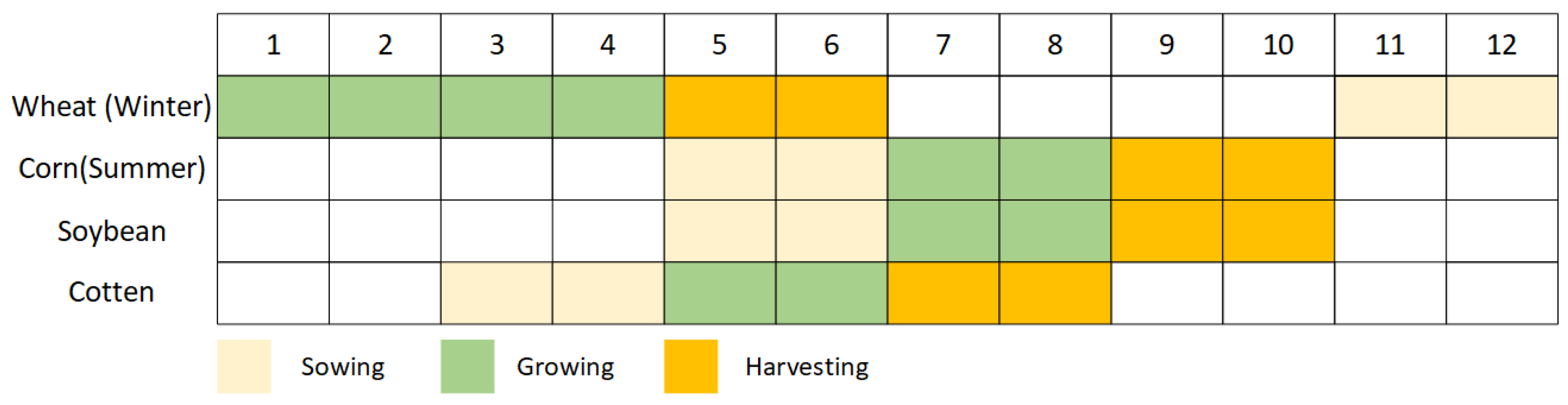
Figure 2 depicts crop calendars for major U.S. crops and shows phenological information for corn and soybeans. By selecting the time zone of the data, crops whose planting time is very different from corn and soybean can be preliminarily distinguished. Because the phenological information of corn and soybeans in autumn is almost the same, the data of corn and soybeans we choose are from 1 August to 31 August [1]. During this period, the plants grow most luxuriantly, and the reflection information on the spectrum is the strongest. At this stage, the band characteristics of different crops are most different and can be efficiently distinguished, which will be introduced in the next subsection.

3.2.2. Spectral Features

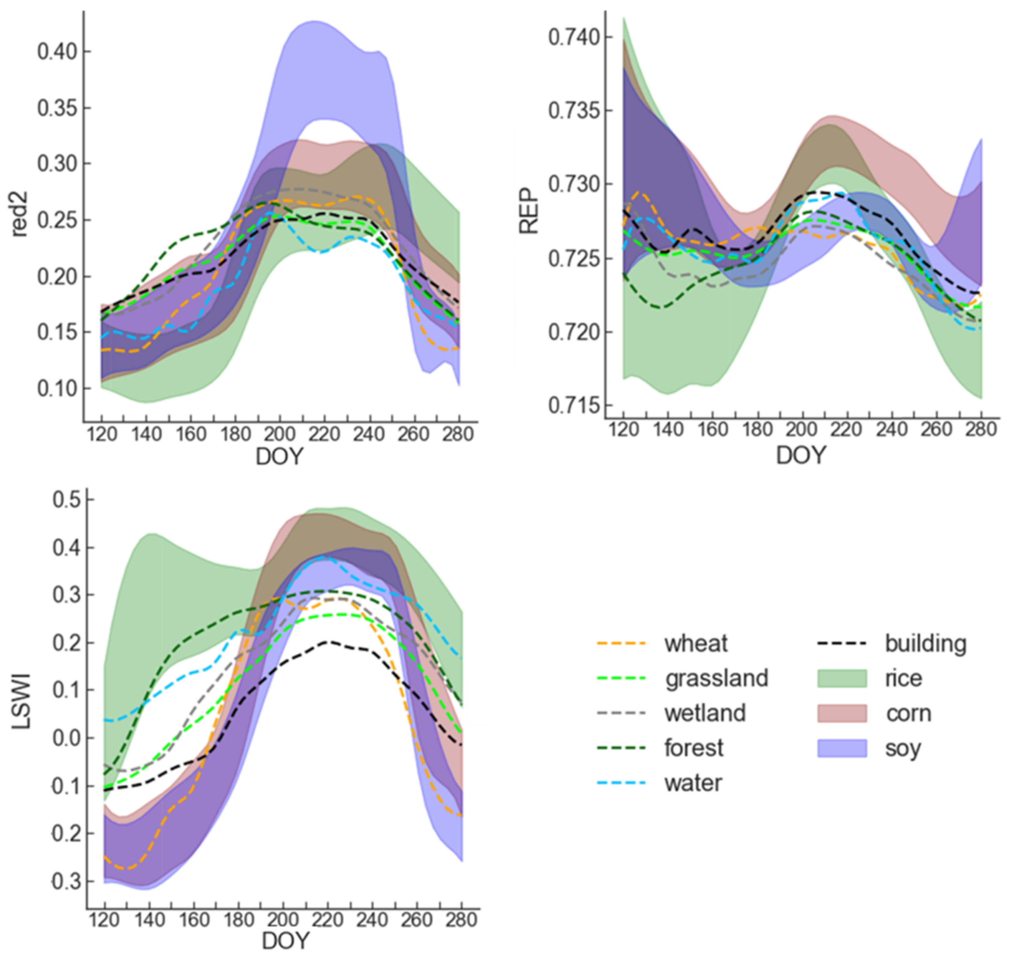
For crops with similar phenological information, spectral information was used to further differentiate them. To select the most suitable vegetation indices for crop mapping, the proposed algorithm utilizes a threshold analysis of the time-series of various commonly used vegetation indices in S2A on different crops and land cover types [25]. Based on this comparison, the Enhanced Vegetation Index Surface Water Index (LSWI) and Red Edge Position (REP) were chosen as the most effective spectral indices (Figure 3) [26,27]. The LSWI is a reliable indicator of vegetation water content, making it useful for differentiating between maize and soybean during the peak growing season. Meanwhile, the REP was found to be helpful in distinguishing between corn and soybean based on the time-series curve. To address the curse of dimensionality and improve the generalization ability of the classifier, the algorithm avoids using other vegetation/water indices and only utilizes the two aforementioned spectral indices. This approach also speeds up the learning process of the classifier. The calculation of the LSWI and REP spectral indices is based on the following formulas:

$$LSWI=\frac{NIR-SWI{R}_1}{NIR+SWI{R}_1}$$

(1)

$$REP=705+35\times \frac{0.5\times (Re{d}_3+Red)-Re{d}_1}{Re{d}_2-Re{d}_1}$$

(2)

where $NIR$ is the reflection value of the near-infrared band; $SWI{R}_1$ is the reflection value of the shortwave infrared band; $Re{d}_3$, $Re{d}_2$, and $Re{d}_1$ are the reflection values of the Red Edge bands with wavelengths of 782.5 nm, 740.2 nm, and 703.9 nm, respectively.

Finally, this algorithm defines the relationship between the reflection threshold of three bands and crops. The two numbers represent the maximum and minimum values, respectively, which are used for all study areas, as shown in

Table 1. The relationship between the reflection and crops.

Time Period [Day]	20 June–20 July	1 July–15 August	1–30 August
	$\mathit{R}\mathit{e}{\mathit{d}}_{\mathbf{2}}$	REP	SWIR1
corn	0.300–0.500	0.727–0.736	0.130–0.180
soybeans	0.230–0.330	0.720–0.730	0.170–0.270

.

3.3. Texture Features

Remote-sensing images are often plagued with the challenge of objects having the same spectrum yet differing characteristics [28,29]. This makes the classification of such images using spectral information alone prone to inaccuracies. However, studies have shown that spatial information, particularly texture features, can enhance the classification accuracy of remote-sensing images [30,31]. Texture features represent the joint distribution of grayscale values of two points with some spatial location relationship. This is achieved by generating a series of spatial variations of the original image on the gray space.

To compute texture features, the co-occurrence matrix is solved based on the grayscale image, and then the partial eigenvalues of the matrix are obtained. Specifically, the GEE platform provides a function called glcmTexture, which computes the texture information based on the grayscale co-occurrence matrix around each pixel in each band. Gray level co-occurrence matrix (GLCM) is defined as the probability of being adjacent to a pixel of value j at a fixed location and orientation from a pixel with the gray value i. The function calculates 14 GLCM metrics constructed by Haralick and four additional metrics designed by Conners. The output comprises 18 bands for each input band if directional averaging is used. Otherwise, there are 18 bands for each directional pair in the kernel. A total of 18 texture features obtained by GLCM of each spectral feature and their meanings are described in

Table 2. Comparison table of 18 feature types and their meanings.

Abbreviation	Full Name and Meaning
ASM	Angular Second Moment, which measures the number of repeated pairs.
CONTRAST	Contrast, which measures the local contrast of an image.
CORR	Correlation, which measures the correlation between pairs of pixels.
VAR	Variance, which measures how spread out the distribution of gray levels is.
IDM	Inverse Difference Moment, which measures the homogeneity.
SAVG	Sum Average,
SVAR	Sum Variance,
SENT	Sum Entropy,
ENT	Entropy, which measures the randomness of a gray-level distribution.
DVAR	Difference variance,
DENT	Difference entropy,
IMCORR1	Information Measure of Corr. 1,
IMCORR2	Information Measure of Corr. 2,
MAXCORR	Max Corr. Coefficient, which is not computed.
DISS	Dissimilarity,
INERTIA	Inertia,
SHADE	Cluster Shade,
PROM	Cluster Prominence.

.

By utilizing texture features, remote-sensing images can be accurately classified, and the limitations of using spectral information alone can be overcome.

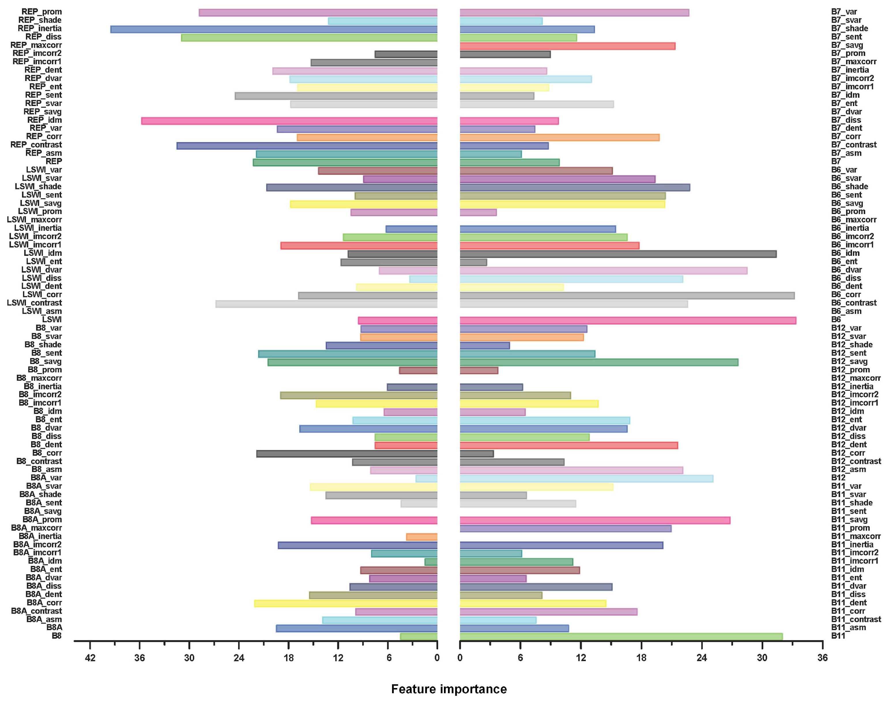
3.4. Importance Analysis

In the pursuit of high-precision classification results, it is essential to optimize feature selection. Incorporating too many features can lead to overfitting, where the model performs exceptionally well on the training data but performs poorly on the test data. Furthermore, using too many features may increase the computational cost and time required to train the model. Hence, the importance of selecting key features for analysis cannot be overstated.

In this study, the importance of the RF classifier is analyzed to obtain importance data for each band. In the test operation, the function ’explain()’ provided by the platform GEE is used to implement the operation. These data serve as the criteria for selecting the most important features for analysis in the three classifiers. This method allows for the identification of high-quality features that are critical for classification while minimizing the number of redundant features.

The data $(\Psi M\Phi ,\Psi N)$ is used to train the $r_{th}$ decision tree $T_r$ in RF, $N_r$ is the number of its leaf nodes. For a specific node, assuming its index is v, the index set of input feature vectors is denoted by $S_{r,v}$, and the components of $\Psi M\Phi$ and $\Psi N$ are denoted as $m_s^r$ and $n_s^r$. On the child node, random and non-repetitive feature selection is performed on the sample, and the features are recorded as $F_{r,v}\in \left\{1,2,\dots ,k\right\}$, where k is the total number of features. The cutting point is recorded as $C_v$, then two complementary subsets can be obtained:

$$\left\{\begin{array}{c}\hfill \begin{array}{c}{S}_{r,v}^{-}=\left\{s\in S_{r,v}\mid m_{s,F_{r,v}}^r\le C_{r,v}\right\}\end{array}\\ \hfill S_{r,v}^{+}=\left\{s\in S_{r,v}\mid m_{s,F_{r,v}}^r>C_{r,v}\right\}\end{array}\right.$$

(3)

When a node is split, the class distribution $N_{r,v,e}$ is split into two parts: $N_{r,v,e}^{-}$ and $N_{r,v,e}^{+}$:

$$\begin{array}{c}\hfill \left\{\begin{array}{c}{N}_{r,v,e}=\frac{1}{S_{r,v}}{\sum }_{s\in S_{r,v}}L(n_s^r=e)\\ N_{r,v,e}^{-}=\frac{1}{S_{r,v}^{-}}{\sum }_{s\in S_{r,v}^{-}}L(n_s^r=e)\\ N_{r,v,e}^{+}=\frac{1}{S_{r,v}^{+}}{\sum }_{s\in S_{r,v}^{+}}L(n_s^r=e)\end{array}\right.\end{array}$$

(4)

The importance of features $F_{r,v}$ in the node v is reflected in the splitting process, where the entropy value is reduced:

$$\begin{array}{c}\hfill {\displaystyle \Gamma \left(F\right)=L(F=F_{r,v})(\sum _{e=1}^E{N}_{r,v,e}{log}_2\frac{1}{N_{r,v,e}}-\sum _{e=1}^E{N}_{r,v,e}^{-}{log}_2\frac{1}{N_{r,v,e}^{-}}-\sum _{e=1}^E{N}_{r,v,e}^{+}{log}_2\frac{1}{N_{r,v,e}^{+}})}\end{array}$$

(5)

The importance of features is inversely proportional to the size of entropy, i.e., the smaller the entropy, the more important the features are. To calculate the importance of F in the entire decision tree, a weighted average of the feature’s contribution at the node is performed using the relative number of samples at each node as a weight:

$$\begin{array}{c}\hfill N_{r,v,e}=\frac{S_{r,v}}{S_r}\end{array}$$

(6)

Then, feature importance is defined as:

$$\begin{array}{c}\hfill {\displaystyle \Gamma \left(F\right)=\frac{1}{\Gamma }\sum _{r=1}^{N_{tree}}\sum _{v=1}^{N_r}{N}_{r,v,e}{\Gamma }_{r,v}\left(F\right)}\end{array}$$

(7)

where $\Gamma$ is the normalization factor:

$$\begin{array}{c}\hfill \Gamma =\underset{F\in \left\{1,2,\dots ,k\right\}}{max}{\displaystyle \sum _{r=1}^{N_{tree}}\sum _{v=1}^{N_r}{N}_{r,v,e}{\Gamma }_{r,v}\left(F\right)}\end{array}$$

(8)

It should be noted that when calculating $\Gamma \left(F\right)$, the predicted category of each sample is not considered, but the category with the highest probability in each leaf node is focused. The principle is that when the data arriving at the child nodes are of the same category, the prediction accuracy of the decision tree will become higher. Entropy serves as a direct measure of this “purity” and helps evaluate the performance of decision trees.

To improve the performance of sub-node splitting and avoid the curse of dimensionality, this section adopts the feature analysis selection method. First, sort the features from high to low importance, and then select the most important feature to form an important feature set. Finally, the classifier is retrained using the important feature set. This algorithm can improve the performance of the model and reduce the number of unnecessary features.

In the preceding section, we retained a total of 152 features, comprising 8 spectral features and 144 texture features. The importance of all features is analyzed, and the results are shown in Figure 4. We take the feature importance analysis results of the random forest classifier on the White area as a reference. Features with high importance values are selected. In this paper, 6 SAVG indices are used as reserved texture features: ‘B6_savg’, ‘B8_savg’, ‘B11_savg’, ‘B12_savg’, ‘REP_savg’, and ‘LSWI_savg’.

3.5. Ensemble Supervised Learning

The present study introduces a novel multi-classifier ensemble algorithm for improving the accuracy and generalization ability of classification models. The proposed approach involves the integration of three different classifiers, namely RF, CART, and SVM, on the GEE platform. In the RF classifier, the parameter variables were initialized with 10 decision trees and a large fraction of 0.1 to ensure optimal performance. The default parameter settings were utilized for CART and SVM classifiers, and they are not reiterated in this paper. It is worth noting that the choice of methodology for surface feature classification affects the sensitivity of the classifier. To address this issue, a multi-classifier ensemble approach is employed, which integrates the classification maps from different classifiers to minimize the possibility of incorrect classification decisions and enhance the overall generalization ability of the models.

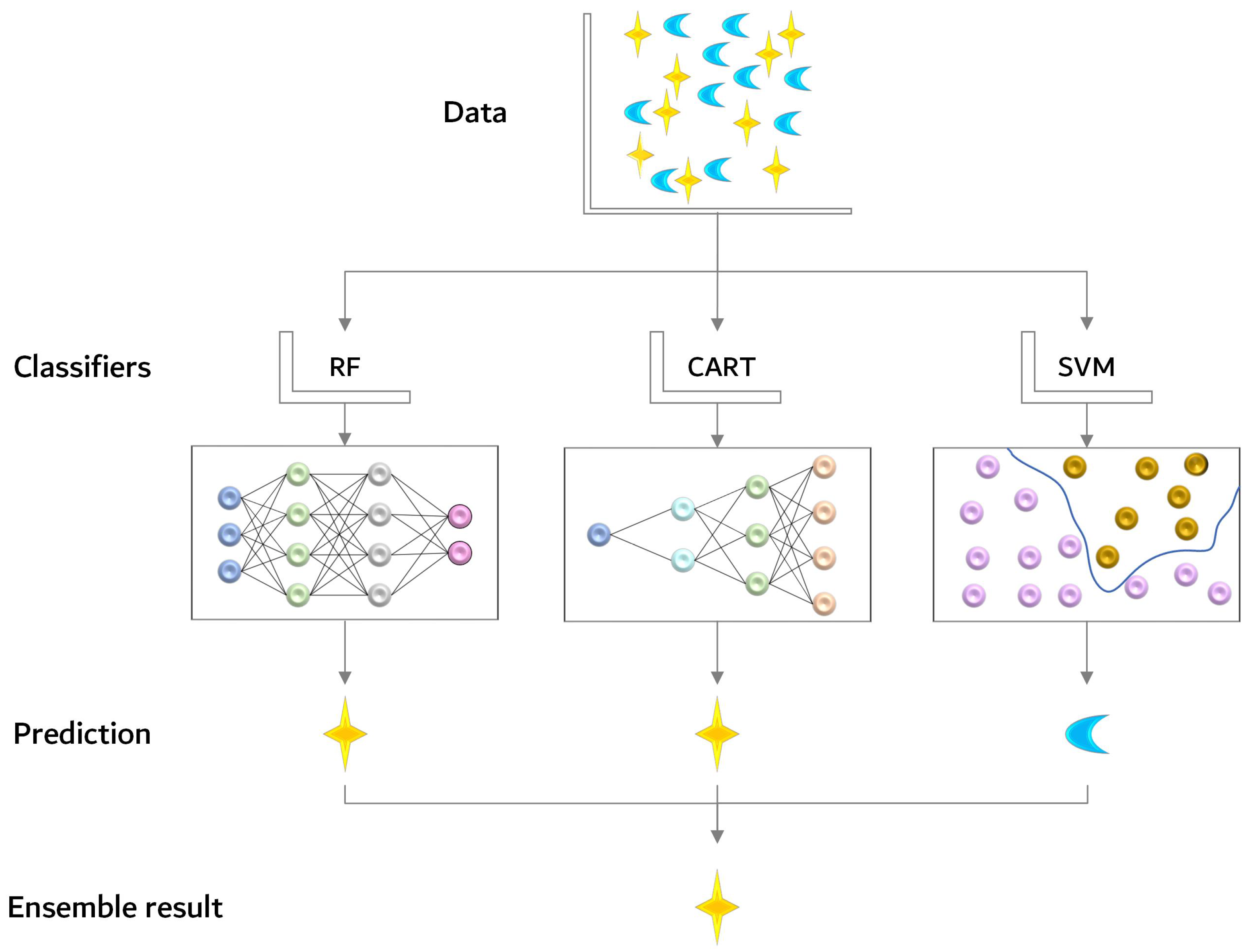
The second proposition of this study is to employ a voting model for decision integration based on multiple classifiers. The voting integration method enables the correction of false predictions generated by weak classifiers through the collective decision of multiple classifiers [32], leading to stable classification models that perform well in all aspects. Specifically, the hard-voting approach is adopted, whereby the voting output is determined based on the predicted results. Treat the prediction result of each base classifier as a vote, vote for each category among all classifiers, and finally, obtain the category with the most votes as the prediction result. The voting process is illustrated in Figure 5.

4. Experiments and Results

4.1. Study Area

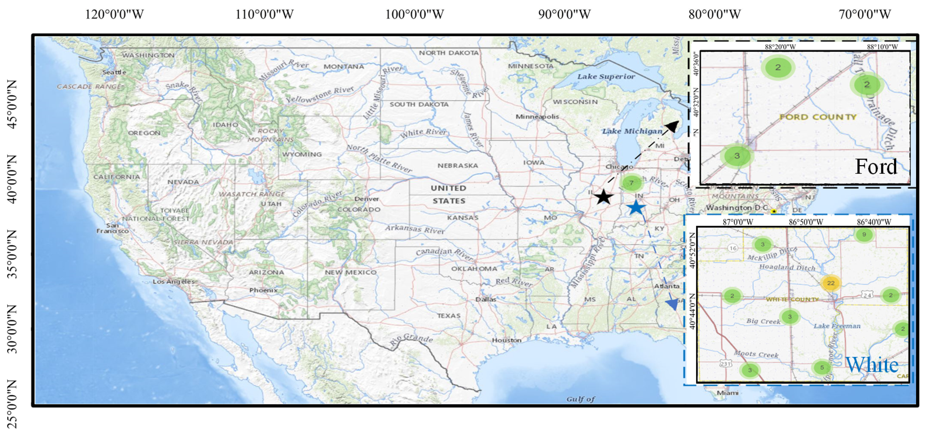
The research areas of this paper are Ford County, Illinois, and White County, Indiana. Their geographical location is shown in Figure 6. Illinois and Indiana are among the top corn and soybean-producing states in the United States, with Illinois being the top soybean-producing state and Indiana being the fifth top corn-producing state in the country. These crops play a critical role in the economic, social, and environmental fabric of these rural communities.

Ford County covers an area of approximately 486 square miles and has a population of around 13,000 residents, according to the United States Census Bureau. The county’s population is primarily concentrated in its largest city, Paxton, which serves as the county seat. The remaining parts of the county consist of small towns and rural areas, where agriculture is the dominant industry.

White County covers a larger area of approximately 510 square miles and has a slightly smaller population of around 25,000 residents, according to the United States Census Bureau. The county is characterized by a mix of agricultural, industrial, and commercial land uses.

4.2. Datasets

The present study utilized two datasets, namely S2A and USDA NASS Cropland Data Layers, which were accessed through the GEE platform. The S2A dataset comprised 23 bands, out of which six bands, namely red edge2, red edge3, red edge4, NIR, SWIR1, and SWIR2, were selected for further processing.

The selection of these bands from the S2A was based on their suitability for vegetation mapping and land cover classification. These bands are known to provide spectral information that is particularly relevant for characterizing different vegetation types and identifying various land cover classes. Furthermore, the use of a subset of bands also reduces computational requirements and processing time while ensuring accurate results for the specific objectives of the study.

The labeled dataset used in the experiment is the USDA NASS Cropland Data Layers, which is a crop-specific land cover data layer created each year for the United States. This data layer was generated using moderate-resolution satellite imagery and extensive agricultural ground-truth data. A total of 254 types of crops were recorded, covering almost all crop types [1].

To prepare the training data for the classification task, the labels corresponding to corn and soybean crops in the USDA NASS Cropland Data Layers were extracted. The value 1 was assigned to the labels corresponding to soybean and corn. The value 0 was assigned to all others. In addition to its use in preparing training data, the USDA NASS Cropland Data Layers was employed as the validation dataset to assess the accuracy of the land cover classification. The resulting classification was compared with the ground-truth data provided by the USDA NASS Cropland Data Layers. The S2A period used as training and test data is from 1 August to 31 August 2019; the USDA NASS Cropland Data period is the entire year of 2019. The S2A period used as verification data is from 1 August to 31 August 2020; the USDA NASS Cropland Data period is the entire year of 2020. The regions corresponding to the training data and the verification data are consistent.

4.3. Evaluation Metrics

A total of 2000 verification sample points were created and divided into two categories. The first category corresponds to locations where crops (either corn or soybean) were planted, and these points were labeled as “1”. The second category corresponds to locations where no corn or soybean was planted, and these points were labeled as “0”. There were 1000 sample points for each category. Each experiment was repeated 10 times. The data obtained are the average of 10 results.

To evaluate the performance of the classification algorithm, four commonly used metrics were adopted: overall accuracy (OA), consumer’s accuracy (CA), producer’s accuracy (PA), and Kappa statistic (K).

OA measures the proportion of correctly classified samples out of all the samples. It is a simple and intuitive metric that provides an overall estimate of classification accuracy.

CA is used to measure the accuracy of a classifier for a certain category, i.e., in a certain category, the proportion of the number of samples correctly classified by the classifier to the total number of samples in the category. It is an important indicator of the credibility of the classifier’s classification results. High consumer accuracy indicates that the classifier has a strong classification ability for the category.

PA represents the authenticity of the classification result of the classifier, i.e., in a certain category given by the classifier, the proportion of the number of samples correctly classified by the classifier to the number of all samples classified into that category. Producer accuracy reflects the ability of the classifier to correctly classify. A high producer precision indicates that the classifier has a strong ability to classify correctly.

K is a measure of agreement between predicted and actual classes, which takes into account the agreement expected by chance.

They are all calculated by the confusion matrix. The confusion matrix is a table that summarizes the performance of a classification algorithm by showing the number of true positives (TP), true negatives (TN), false positives (FP), and false negatives (FN) that were obtained, which is shown in

Table 3. The confusion matrix.

Actual∖Predicted	1 (Crop)	0 (No Crop)	Row Total
1 (Crop)	TP	FN	1000
0 (No Crop)	FP	TN	1000
Column total	TP+FP	FN+TN	2000

. Each row in the matrix represents the instances in a predicted class, while each column represents the instances in an actual class.

$$OA=\frac{TP+TN}{TP+TN+FP+FN}$$

(9)

$$CA=\frac{TP}{TP+FN} or \frac{FP}{FP+TN}$$

(10)

$$PA=\frac{TP}{TP+FP} or \frac{FN}{FN+TN}$$

(11)

$$K=\frac{N\times (TP+TN)-(TP+FP)\times (TP+FN)}{N^2-(TP+FP)\times (TP+FN)}$$

(12)

where N is the total number of samples.

4.4. Overall Performance

The classification accuracy of the proposed algorithm for the two crops in the two research areas is shown in

Table 4. Corn classification results in Ford.

	Classifier	TN	TP	OA(%)	CA		PA		K
					0	1	0	1
	RF	915	694	80.45	0.915	0.694	0.749	0.891	0.609
	CART	886	693	78.95	0.886	0.693	0.743	0.859	0.579
	SVM	899	718	80.85	0.899	0.718	0.761	0.877	0.617
After spectral information extraction	RF	911	717	81.4	0.911	0.717	0.763	0.890	0.628
	CART	868	729	79.85	0.868	0.729	0.743	0.859	0.579
	SVM	900	716	0.592	0.9	0.716	0.760	0.877	0.616
Using CSA	RF	910	713	81.15	0.91	0.713	0.76	0.888	0.623
	CART	851	716	78.35	0.851	0.716	0.750	0.828	0.567
	SVM	918	674	79.6	0.918	0.674	0.752	0.886	0.592
	Collective decision	914	718	81.6	0.914	0.718	0.764	0.893	0.632

,

Table 5. Soybean classification results in Ford.

	Classifier	TN	TP	OA(%)	CA		PA		K
					0	1	0	1
	RF	748	882	81.5	0.748	0.882	0.864	0.778	0.623
	CART	748	849	79.85	0.748	0.849	0.832	0.771	0.597
	SVM	729	907	81.8	0.729	0.907	0.887	0.770	0.636
After spectral information extraction	RF	772	873	82.25	0.772	0.873	0.859	0.793	0.645
	CART	767	841	80.4	0.767	0.841	0.829	0.783	0.608
	SVM	705	900	80.25	0.705	0.9	0.876	0.753	0.605
Using CSA	RF	804	878	84.1	0.804	0.878	0.868	0.816	0.682
	CART	779	831	80.5	0.779	0.831	0.822	0.790	0.61
	SVM	732	903	81.75	0.732	0.903	0.883	0.771	0.635
	Collective decision	790	892	84.1	0.79	0.892	0.880	0.809	0.682

,

Table 6. Corn classification results in White.

	Classifier	TN	TP	OA(%)	CA		PA		K
					0	1	0	1
	RF	882	742	62.4	0.882	0.742	0.774	0.863	0.624
	CART	778	767	77.25	0.778	0.767	0.770	0.776	0.545
	SVM	850	775	81.25	0.85	0.775	0.791	0.838	0.625
After spectral information extraction	RF	901	752	82.65	0.901	0.752	0.784	0.884	0.653
	CART	763	796	77.95	0.763	0.796	0.789	0.771	0.559
	SVM	901	769	83.5	0.901	0.769	0.796	0.886	0.670
Using CSA	RF	893	781	83.7	0.893	0.781	0.803	0.880	0.674
	CART	774	790	78.2	0.774	0.79	0.787	0.778	0.564
	SVM	914	768	84.1	0.914	0.768	0.800	0.900	0.682
	Collective decision	912	785	84.85	0.912	0.785	0.809	0.889	0.697

and

Table 7. Soybean classification results in White.

	Classifier	TN	TP	OA(%)	CA		PA		K
					0	1	0	1
	RF	846	756	80.1	0.846	0.756	0.776	0.831	0.602
	CART	850	722	78.6	0.850	0.722	0.754	0.83	0.572
	SVM	940	683	81.15	0.940	0.683	0.748	0.919	0.623
After spectral information extraction	RF	914	700	80.7	0.914	0.700	0.752	0.89	0.614
	CART	847	715	78.1	0.847	0.715	0.748	0.824	0.562
	SVM	943	679	81.1	0.943	0.679	0.746	0.923	0.622
Using CSA	RF	929	696	62.5	0.929	0.696	0.753	0.907	0.625
	CART	845	754	79.95	0.845	0.754	0.775	0.830	0.599
	SVM	909	728	81.85	0.909	0.728	0.770	0.889	0.637
	Collective decision	932	715	82.35	0.932	0.715	0.766	0.913	0.647

. The OA and K with the best results in each category are highlighted in bold.

It can be seen that among the four tables, the results of decision voting are the best, which proves the effectiveness and robustness of the proposed algorithm. First, comparing the performance of the spectral feature-processed data on the three classifiers with the original data, the OA of the former is improved by 1–2% on average, although the OA of the latter is higher in a few experiments. Second, the OA after CSA processing is 2–3% higher than the OA after spectral feature processing on average. In the end, the decision result is much better than the original classification result. OA is increased by 2–3%. K increased by 0.03–0.06.

When doing soybean classification in the Ford, the accuracy obtained by the random forest algorithm processed by spectral information is as good as the decision voting. We think it is because the OA of the CART classifier is 7% lower than that of the RF classifier. The input of unbalanced classification results affects the ensemble result.

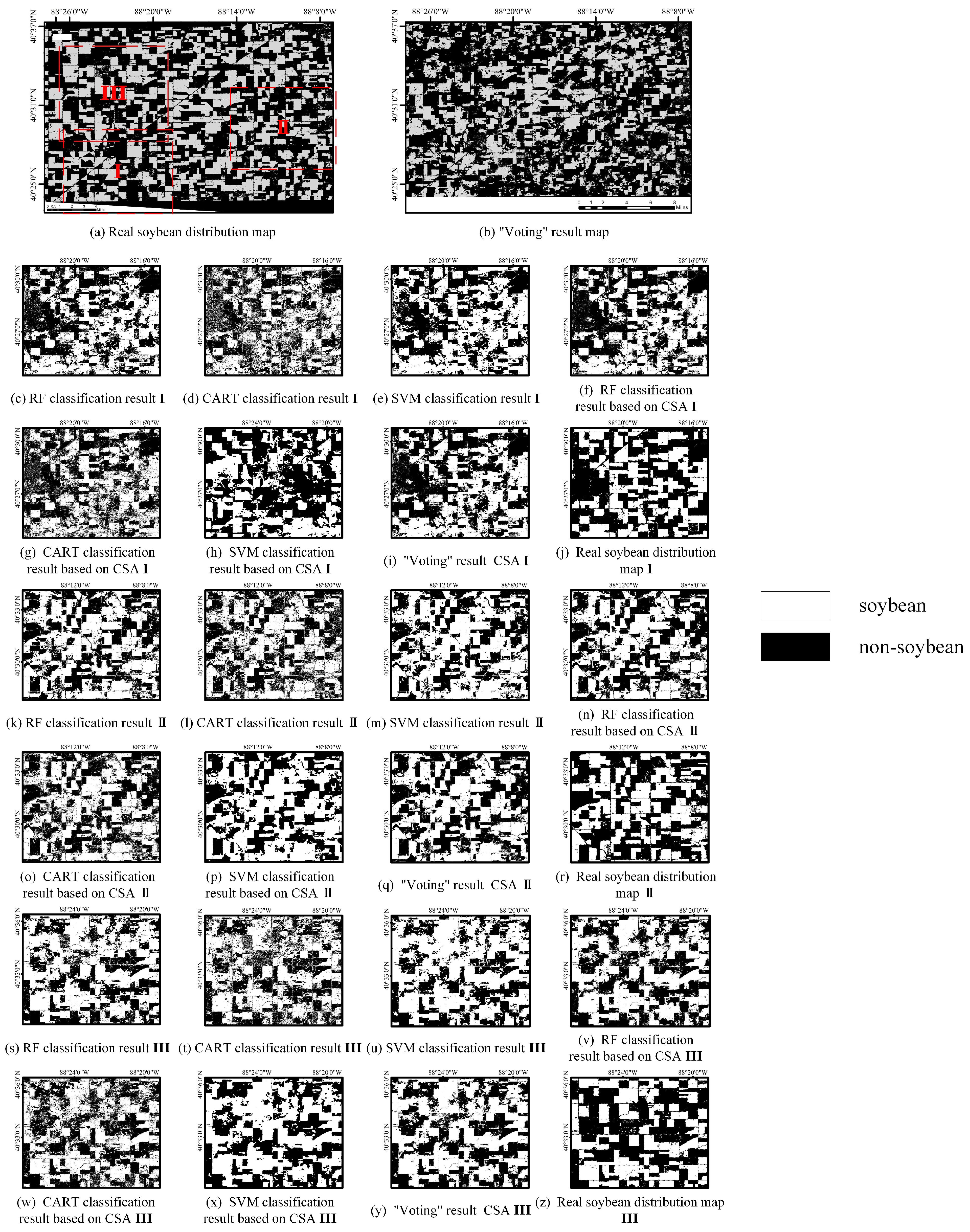
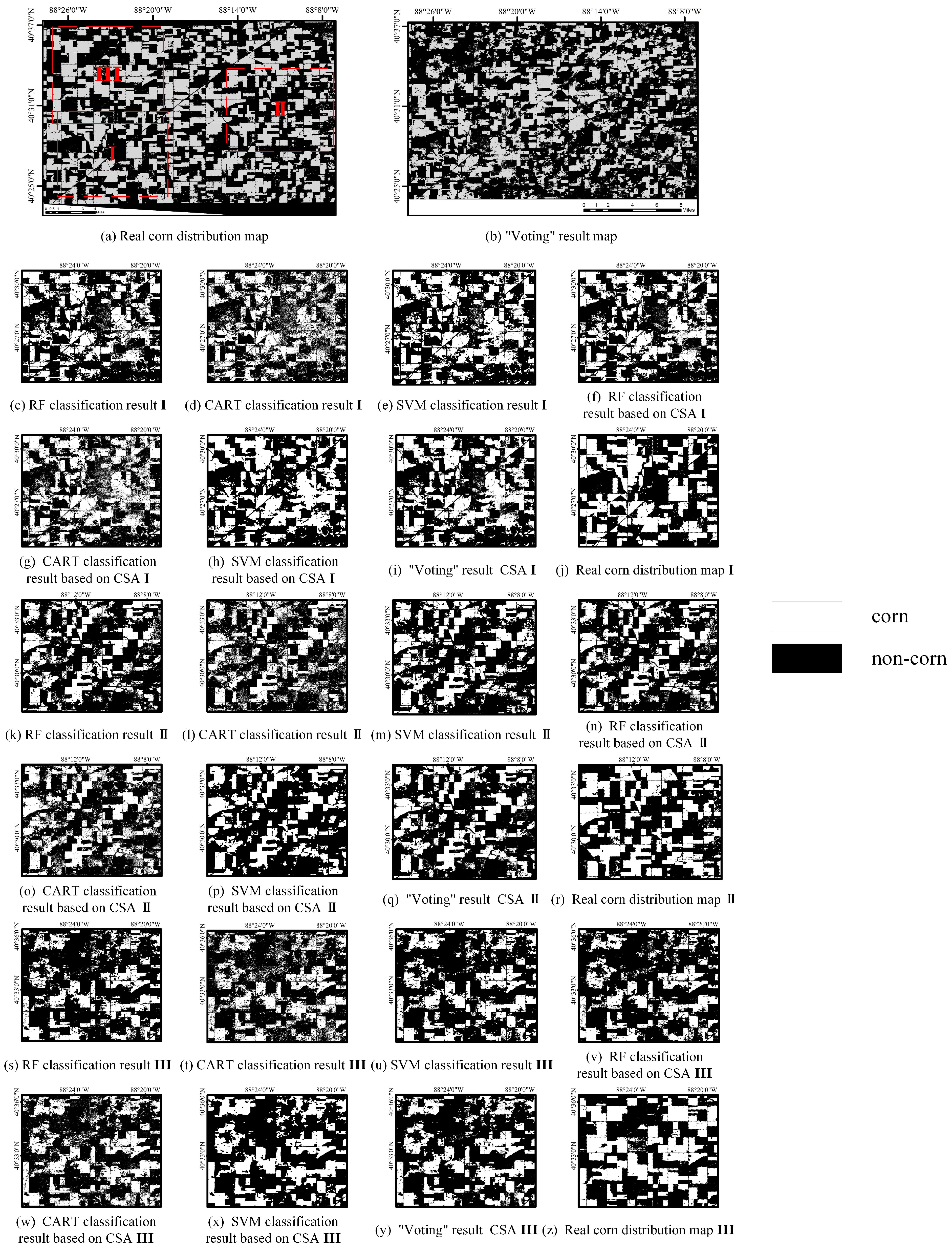
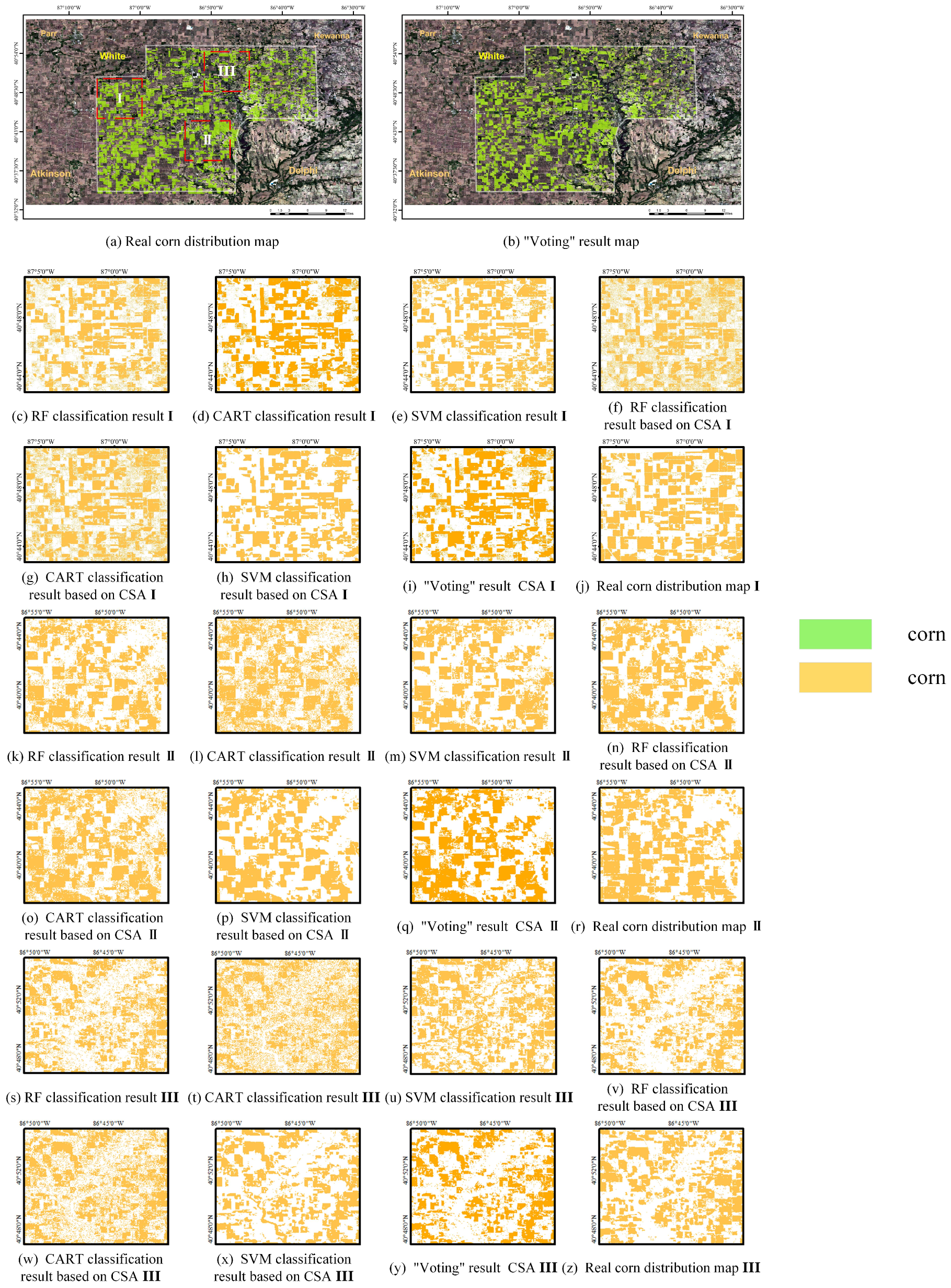
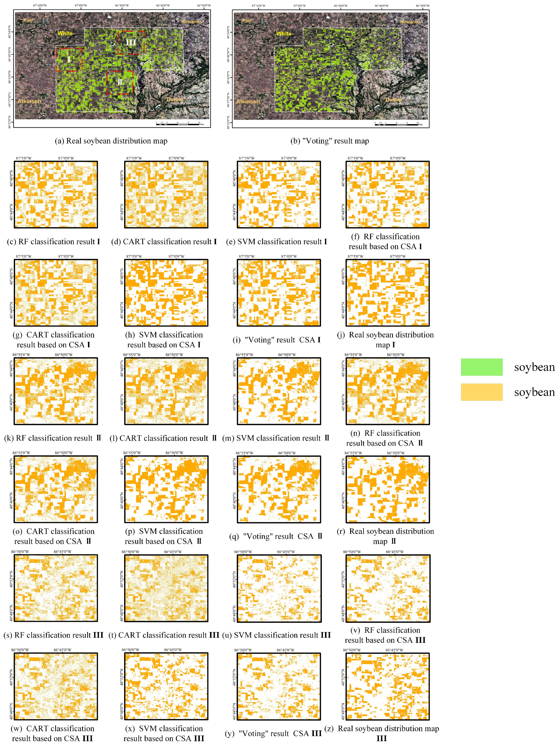
Three parts of each study area were selected for image enlargement for comparison. All classified maps are shown in Figure 7, Figure 8, Figure 9 and Figure 10. In the result maps of the Ford area (Figure 7 and Figure 8), the white part is the crop planting area, and the black part is the non-crop planting area. In the result maps of the White area (Figure 9 and Figure 10), the background is the satellite image of the area, and the green and orange masks are the crop planting areas. It can be seen that the edges of the plots are not clear in the classification map of the original classifier. Large areas of land parcels are not fully detected compared to real maps. It appears more fragmented. The classification map after CSA processing is better. Obviously, the large planting areas are detected more completely. Especially for the maps that have passed the decision-making vote, there is less black area in the middle of the large-scale planting areas. The edges of planted areas are much clearer.

5. Discussion

Integration of spatial and spectral features offers several benefits for crop classification, including improved accuracy and reduced misclassification. Spatial features provide information on the spatial arrangement of land cover classes, while spectral features capture the differences in reflectance characteristics between classes. By combining these two types of features, the algorithm can better discriminate between classes, especially in complex landscapes where crops may be intermingled with other vegetation types or have similar spectral properties. This integration can also help overcome some of the limitations of using only spectral features, such as confusion between classes with similar spectral signatures.

In summary, feature selection is crucial in achieving high-quality classification results. The GEE platform’s “explain” module enables the identification of important texture and spectral features for analysis. The RF classifier’s importance analysis provides the selection criteria for the three classifiers, ensuring the selection of the most critical features for analysis while optimizing computational efficiency. Feature importance analysis can help identify which features are most relevant for classification and thus optimize the use of computational resources. Our results show that the maxcorr texture feature is not useful for classifying crops, while the SAVG textures are important. This indicates that the algorithm should focus on extracting and using these features for classification while avoiding the inclusion of irrelevant or redundant features. Then, the algorithm can achieve higher accuracy while minimizing computational costs.

The three classifiers used as base classifiers are trained with the integrated spatial and spectral features, and the collective voting decision is taken for the final classification. This decision-making process takes into account the diverse and complementary strengths of the three classifiers and reduces the risk of overfitting that may occur when using a single classifier. Moreover, the ensemble of the three classifiers improves the performance of the algorithm in handling complex scenarios that may involve variations in environmental conditions and data acquisition issues.

The decision integration step is critical for achieving accurate and reliable classification results. However, the use of decision voting may not always be appropriate, especially when there are significant differences in the classification levels of the base classifiers. In such cases, a poor classifier may actually reduce the accuracy of the algorithm. Therefore, it is important to carefully evaluate the performance of each classifier and consider their relative strengths and weaknesses before deciding on the appropriate method for decision ensemble.

Leveraging the foundational insights extracted from the pioneering endeavors of papers [1,33], our algorithm embarks on a formidable extension, transcending the confines of single-crop classification. Where [1] focused on the categorization of a singular crop, our methodology ventures boldly into the realm of dual-crop classification, paving the way for a paradigm shift in agricultural mapping and classification practices. The classification performance of the proposed algorithm is good. The OA is around 0.80. Compared with [34], the accuracy is higher. Enriching the number of features will help improve classification accuracy. Although dozens of features were added to [35] and their importance was evaluated, the features were not screened. This results in an increase in the number of features but a decrease in OA. This paper adds a feature selection step. When the number of features is several times less than that, OA is improved to the same extent. Through the intricate fusion of machine learning and ensemble learning techniques, our proposed feature-level classification algorithm showcases not only robustness and generalizability but also pioneers the integration of multi-crop classification methodologies, enriching the landscape of precision agriculture and food security initiatives.

6. Conclusions

In this paper, a decision ensemble-based algorithm for classifying corn and soybean crops in Google Earth Engine is proposed. The algorithm integrates spatial and spectral features extracted from S2A, and three supervised classifiers are employed as base classifiers to achieve improved classification accuracy. The method is tested on two study areas for two kinds of crops. Experimental results showed that the proposed approach achieved high classification accuracy, with the decision-voting strategy outperforming the individual classifiers. The classification accuracy is improved by an average of 2–3 % compared to the original classifications. The Kappa coefficient has been improved by 3–6 %. In summary, the use of a decision ensemble-based approach and the integration of spatial and spectral features have demonstrated the potential to improve classification accuracy, reliability, and robustness.

References

- Wang, S.; Feng, W.; Quan, Y.; Li, Q.; Dauphin, G.; Huang, W.; Li, J.; Xing, M. A heterogeneous double ensemble algorithm for soybean planting area extraction in Google Earth Engine. Comput. Electron. Agric. 2022, 197, 106955. [Google Scholar] [CrossRef]
- Hrustek, L. Sustainability driven by agriculture through digital transformation. Sustainability 2020, 12, 8596. [Google Scholar] [CrossRef]
- Garske, B.; Bau, A.; Ekardt, F. Digitalization and AI in European agriculture: A strategy for achieving climate and biodiversity targets? Sustainability 2021, 13, 4652. [Google Scholar] [CrossRef]
- Barela, A.; Thakur, S.; Pachori, S.; Rahangdale, S.; Goyal, V.K.; Kakade, S.; Shrivastava, M. Applications of proximal remote sensing in agriculture: A review. Pharma Innov. J. 2023, 12, 1124–1130. [Google Scholar]
- Tantalaki, N.; Souravlas, S.; Roumeliotis, M. Data-driven decision making in precision agriculture: The rise of big data in agricultural systems. J. Agric. Food Inf. 2019, 20, 344–380. [Google Scholar] [CrossRef]
- Ali, I.; Mushtaq, Z.; Arif, S.; Algarni, A.D.; Soliman, N.F.; El-Shafai, W. Hyperspectral images-based crop classification scheme for agricultural remote sensing. Comput. Syst. Sci. Eng. 2023, 46, 303–319. [Google Scholar] [CrossRef]
- Yuan, Y.; Lin, L.; Zhou, Z.G.; Jiang, H.; Liu, Q. Bridging optical and SAR satellite image time series via contrastive feature extraction for crop classification. ISPRS J. Photogramm. Remote Sens. 2023, 195, 222–232. [Google Scholar] [CrossRef]
- You, N.; Dong, J.; Li, J.; Huang, J.; Jin, Z. Rapid early-season maize mapping without crop labels. Remote Sens. Environ. 2023, 290, 113496. [Google Scholar] [CrossRef]
- Farmonov, N.; Amankulova, K.; Szatmári, J.; Sharifi, A.; Abbasi-Moghadam, D.; Nejad, S.M.M.; Mucsi, L. Crop type classification by DESIS hyperspectral imagery and machine learning algorithms. IEEE J. Sel. Top. Appl. Earth Obs. Remote Sens. 2023, 16, 1576–1588. [Google Scholar] [CrossRef]
- Misra, N.; Dixit, Y.; Al-Mallahi, A.; Bhullar, M.S.; Upadhyay, R.; Martynenko, A. IoT, big data, and artificial intelligence in agriculture and food industry. IEEE Internet Things J. 2020, 9, 6305–6324. [Google Scholar] [CrossRef]
- Kaya, E.; Agca, M.; Adiguzel, F.; Cetin, M. Spatial data analysis with R programming for environment. Hum. Ecol. Risk Assess. Int. J. 2019, 25, 1521–1530. [Google Scholar] [CrossRef]
- Gorelick, N.; Hancher, M.; Dixon, M.; Ilyushchenko, S.; Thau, D.; Moore, R. Google Earth Engine: Planetary-scale geospatial analysis for everyone. Remote Sens. Environ. 2017, 202, 18–27. [Google Scholar] [CrossRef]
- Tamiminia, H.; Salehi, B.; Mahdianpari, M.; Quackenbush, L.; Adeli, S.; Brisco, B. Google Earth Engine for geo-big data applications: A meta-analysis and systematic review. ISPRS J. Photogramm. Remote Sens. 2020, 164, 152–170. [Google Scholar] [CrossRef]
- Yang, Y.; Yang, D.; Wang, X.; Zhang, Z.; Nawaz, Z. Testing accuracy of land cover classification algorithms in the qilian mountains based on gee cloud platform. Remote Sens. 2021, 13, 5064. [Google Scholar] [CrossRef]
- Capolupo, A.; Monterisi, C.; Caporusso, G.; Tarantino, E. Extracting land cover data using GEE: A review of the classification indices. In Proceedings of the Computational Science and Its Applications–ICCSA 2020: 20th International Conference, Cagliari, Italy, 1–4 July 2020; Proceedings, Part IV 20. Springer: Berlin/Heidelberg, Germany, 2020; pp. 782–796. [Google Scholar]
- Hu, L.; Shariff, A.R.B.M.; Omar, H.; Song, D.X.; Wu, H. GEE-Based Spatiotemporal Evolution of Deforestation Monitoring in Malaysia and Its Drivers. In Remote Sensing Application: Regional Perspectives in Agriculture and Forestry; Springer: Berlin/Heidelberg, Germany, 2022; pp. 279–302. [Google Scholar]
- Han, J.; Zhang, Z.; Cao, J.; Luo, Y.; Zhang, L.; Li, Z.; Zhang, J. Prediction of winter wheat yield based on multi-source data and machine learning in China. Remote Sens. 2020, 12, 236. [Google Scholar] [CrossRef]
- DeVries, B.; Huang, C.; Armston, J.; Huang, W.; Jones, J.W.; Lang, M.W. Rapid and robust monitoring of flood events using Sentinel-1 and Landsat data on the Google Earth Engine. Remote Sens. Environ. 2020, 240, 111664. [Google Scholar] [CrossRef]
- Mekha, P.; Teeyasuksaet, N. Image Classification of Rice Leaf Diseases Using Random Forest Algorithm. In Proceedings of the 2021 Joint International Conference on Digital Arts, Media and Technology with ECTI Northern Section Conference on Electrical, Electronics, Computer and Telecommunication Engineering, Cha-am, Thailand, 3–6 March 2021; pp. 165–169. [Google Scholar] [CrossRef]
- Feng, W.; Quan, Y.; Dauphin, G.; Li, Q.; Gao, L.; Huang, W.; Xia, J.; Zhu, W.; Xing, M. Semi-supervised rotation forest based on ensemble margin theory for the classification of hyperspectral image with limited training data. Inf. Sci. 2021, 575, 611–638. [Google Scholar] [CrossRef]
- Fan, X.; Feng, Z.; Yang, X.; Xu, T.; Tian, J.; Lv, N. Haze weather recognition based on multiple features and Random Forest. In Proceedings of the 2018 International Conference on Security, Pattern Analysis, and Cybernetics (SPAC), Jinan, China, 14–17 December 2018; pp. 485–488. [Google Scholar] [CrossRef]
- Gavankar, S.S.; Sawarkar, S.D. Eager decision tree. In Proceedings of the 2017 2nd International Conference for Convergence in Technology (I2CT), Mumbai, India, 7–9 April 2017; pp. 837–840. [Google Scholar] [CrossRef]
- Chen, P. The Application of an Improved C4.5 Decision Tree. In Proceedings of the 2021 7th Annual International Conference on Network and Information Systems for Computers (ICNISC), Guiyang, China, 23–25 July 2021; pp. 392–396. [Google Scholar] [CrossRef]
- Wu, X.; Zuo, W.; Lin, L.; Jia, W.; Zhang, D. F-SVM: Combination of Feature Transformation and SVM Learning via Convex Relaxation. IEEE Trans. Neural Netw. Learn. Syst. 2018, 29, 5185–5199. [Google Scholar] [CrossRef] [PubMed]
- You, N.; Dong, J. Examining earliest identifiable timing of crops using all available Sentinel 1/2 imagery and Google Earth Engine. ISPRS J. Photogramm. Remote Sens. 2020, 161, 109–123. [Google Scholar] [CrossRef]
- E.D. Chaves, M.; C.A. Picoli, M.; D. Sanches, I. Recent Applications of Landsat 8/OLI and Sentinel-2/MSI for Land Use and Land Cover Mapping: A Systematic Review. Remote Sens. 2020, 12, 3062. [Google Scholar] [CrossRef]
- Ali, A.; Imran, M. Evaluating the potential of red edge position (REP) of hyperspectral remote sensing data for real time estimation of LAI & chlorophyll content of kinnow mandarin (Citrus reticulata) fruit orchards. Sci. Hortic. 2020, 267, 109326. [Google Scholar] [CrossRef]
- Hong, D.; Yokoya, N.; Chanussot, J.; Zhu, X.X. An Augmented Linear Mixing Model to Address Spectral Variability for Hyperspectral Unmixing. IEEE Trans. Image Process. 2019, 28, 1923–1938. [Google Scholar] [CrossRef]
- Liang, M.; Jiao, L.; Yang, S.; Liu, F.; Hou, B.; Chen, H. Deep Multiscale Spectral-Spatial Feature Fusion for Hyperspectral Images Classification. IEEE J. Sel. Top. Appl. Earth Obs. Remote Sens. 2018, 11, 2911–2924. [Google Scholar] [CrossRef]
- Cheng, G.; Ding, H.; Yang, J.; Cheng, Y. Crop type classification with combined spectral, texture, and radar features of time-series Sentinel-1 and Sentinel-2 data. Int. J. Remote Sens. 2023, 44, 1215–1237. [Google Scholar] [CrossRef]
- Luo, K.; Lu, L.; Xie, Y.; Chen, F.; Yin, F.; Li, Q. Crop type mapping in the central part of the North China Plain using Sentinel-2 time series and machine learning. Comput. Electron. Agric. 2023, 205, 107577. [Google Scholar] [CrossRef]
- Feng, W.; Quan, Y.; Dauphin, G. Label noise cleaning with an adaptive ensemble method based on noise detection metric. Sensors 2020, 20, 6718. [Google Scholar] [CrossRef]
- Chen, S.; Woodcock, C.E.; Bullock, E.L.; Arévalo, P.; Torchinava, P.; Peng, S.; Olofsson, P. Monitoring temperate forest degradation on Google Earth Engine using Landsat time series analysis. Remote Sens. Environ. 2021, 265, 112648. [Google Scholar] [CrossRef]
- Luo, C.; Liu, H.J.; Lu, L.P.; Liu, Z.R.; Kong, F.-C.; Zhang, X.-L. Monthly composites from Sentinel-1 and Sentinel-2 images for regional major crop mapping with Google Earth Engine. J. Integr. Agric. 2021, 20, 1944–1957. [Google Scholar] [CrossRef]
- Kobayashi, N.; Tani, H.; Wang, X.; Sonobe, R. Crop classification using spectral indices derived from Sentinel-2A imagery. J. Inf. Telecommun. 2020, 4, 67–90. [Google Scholar] [CrossRef]
Figure 1.
The algorithm flowchart.
Figure 2.
Phenological calendars for common crops.
Figure 3.
Time-series spectral band information for crops [25].
Figure 4.
Analysis of the importance of RF features in White. The value in the graph is the visualization of the importance of the feature, and the higher the value, the more important the feature.
Figure 5.
Collective voting process. Different patterns and colors represent different classes or classification features.
Figure 6.
The locations of two study areas.
Figure 7.
Corn maps of Ford. The white part is the predicted/real soybean planting area. Figure (a) is the ground truth, and Figure (b) is the classification diagram of the algorithm proposed in this article. (c–j) are the local enlarged comparison pictures of different algorithms and ground truth in the I part. (k–r) are the partially enlarged comparison pictures and ground truth of different algorithms in the II part. (s–z) are the partially enlarged comparison pictures and ground truth of different algorithms in the III part.
Figure 8.
Soybean maps of Ford. The white part is the predicted/real soybean planting area. Figure (a) is the ground truth, and Figure (b) is the classification diagram of the algorithm proposed in this article. (c–j) are the local enlarged comparison pictures of different algorithms and ground truth in the I part. (k–r) are the partially enlarged comparison pictures and ground truth of different algorithms in the II part. (s–z) are the partially enlarged comparison pictures and ground truth of different algorithms in the III part.
Figure 9.
Corn maps of White. The green parts and orange parts are the predicted/real corn planting areas. The white line is the area boundary. Figure (a) is the ground truth, and Figure (b) is the classification diagram of the algorithm proposed in this article. (c–j) are the local enlarged comparison pictures of different algorithms and ground truth in the I part. (k–r) are the partially enlarged comparison pictures and ground truth of different algorithms in the II part. (s–z) are the partially enlarged comparison pictures and ground truth of different algorithms in the III part.
Figure 10.
Soybean maps of White. The green parts and orange parts are the predicted/real soybean planting areas. The white line is the area boundary. Figure (a) is the ground truth, and Figure (b) is the classification diagram of the algorithm proposed in this article. (c–j) are the local enlarged comparison pictures of different algorithms and ground truth in the I part. (k–r) are the partially enlarged comparison pictures and ground truth of different algorithms in the II part. (s–z) are the partially enlarged comparison pictures and ground truth of different algorithms in the III part.