
On the Use of Ultra-WideBand-Based Augmentation for Precision Maneuvering
by
 , , , and
Paul Zabalegui
1,2,
Gorka De Miguel
1,2,
Nerea Fernández-Berrueta
1,2,
Joanes Aizpuru
1,2,
Jaizki Mendizabal
1,2 and
Iñigo Adín
1,2,* 1
CEIT-Basque Research and Technology Alliance (BRTA), Manuel Lardizabal 15, 20018 Donostia/San Sebastián, Spain
2
Tecnun, School of Engineering, Department of Electric and Electronical engineering, Universidad de Navarra, Manuel Lardizabal 13, 20018 Donostia/San Sebastián, Spain
*
Author to whom correspondence should be addressed.
Remote Sens. 2024, 16(5), 911; https://doi.org/10.3390/rs16050911
Submission received: 31 October 2023
/
Revised: 20 February 2024
/
Accepted: 29 February 2024
/
Published: 4 March 2024
(This article belongs to the Special Issue GNSS for Urban Transport Applications II)
Abstract
:The limitations of the existing Global Navigation Satellite Systems (GNSS) integrated with Inertial Measurement Units (IMU) have presented significant challenges in meeting the stringent demands of precision maneuvering. The identified constraints in terms of accuracy and availability have required the development of an alternative solution to enhance the performance of navigation systems in dynamic and diverse environments. This paper summarizes the research regarding the integration of ultra-wideband (UWB) technology as an augmentation of the conventional GNSS+IMU system; it proposes an approach that aims to overcome the limitations of conventional navigation systems. By making use of UWB technology, the proposed low-cost UWB-augmented GNSS+IMU system not only fulfils the required performance standards but also offers the unique capability to navigate seamlessly across indoor and outdoor environments. The developed system was validated through comprehensive testing and analysis in both the automotive and maritime sectors. The obtained results highlight the system’s capacity as a dependable and resilient solution for precise navigation, and they promote its use within the domain of accurate maneuvering.
1. Introduction
Due to the unprecedented advancements in transportation technologies, precise and reliable navigation systems have become part of the foundation of modern transportation and mobility. In every transportation sector, such as the automotive and maritime sectors and even the aviation sector, the ability to accurately determine a vehicle’s position and orientation in real time has completely changed not only the way we move but also the way we live.
In the last decades, Global Navigation Satellite Systems (GNSS) and Inertial Measurement Units (IMU) have played fundamental roles in the navigation world. GNSS has provided global positioning information to almost every corner of the globe, while IMUs, which rely on accelerometers and gyroscopes, offer continuous updates on orientation and movement. The fusion of these two technologies has made possible a wide variety of applications, ranging from those used in air travel and maritime shipping to those used in terrestrial navigation in the automotive domain [1,2].
However, as the requirements for navigation systems have significantly grown, conventional GNSS+IMU-based solutions have faced multiple new challenges, such as the need for higher availability or seamless navigation in indoor/outdoor transitions in which this architecture may not excel [3,4]. Precision maneuvering, such as the safe operation of autonomous vehicles or the delicate task of docking boats in confined spaces, requires such accuracy and reliability that common commercial technologies often cannot meet the requirements.
As a response to these challenges, multiple technologies and proposals have emerged [5,6] as promising augmentation systems for GNSS+IMU-based navigation, of which ultra-wideband (UWB) technology is an example. UWB is a radio technology seen as a reliable option when trying to address the primary limitations of GNSS in situations with limited visibility. This is due to its sub-meter accuracy and the tailored transmitting anchor setup it offers, which converts it into a reliable source of information for vehicle positioning, enhancing productivity on assembly lines, and asset tracking in warehouses, among other applications [7,8,9,10,11,12,13]. Previous research shows that, due to the fact that UWB technology is analogous to GNSS in terms of its trilateration principle, they can be fused by employing different algorithms and strategies [10,14,15]. In addition, research has been conducted with the aim of using UWB augmentation for a faster obtention of real-time kinematics (RTK) fixed solutions [16,17], using loosely coupled fusions for multisensor pedestrian navigation [18] and even for the design of error-avoiding methods for sensor integration in controlled lab environments [19]. The authors in [20] propose a GNSS+INS+UWB+Map integration in which RTK is also employed to obtain higher accuracies; thus, UWB is not employed as an augmentation system but as a way of increasing solution availability indoors. The research work in [21] proposes a two-stage filter in which a GNSS+INS+UWB layer aids a second GNSS+INS to improve its position, which is then tested in a controlled lab environment. Lastly, [22] does employ UWB as an augmentation system for a GNSS+IMU approach, but with the aim of solving GNSS outages using a two-stage extended Kalman filter (EKF).
This scientific paper explores the integration of UWB as an augmentation technology for GNSS+IMU-based navigation systems by means of a single error-state EKF, addressing the pressing need for improved accuracy and performance in transportation applications. For this purpose, a tightly coupled dual-constellation (GPS+GALILEO) GNSS+IMU+UWB algorithm was implemented to test the influence of a low-cost technology such as UWB as an augmentation method for a low-cost GNSS+IMU navigation system. This algorithm was tested in real-world scenarios by installing the mentioned low-cost system in some of the most employed means of transport, such as those used in the automotive and maritime sectors, and by employing two different UWB anchor geometries. These tests took place in dynamic scenarios, such as the entrance to a garage in a suburban environment and Bilbao’s commercial port, which handles various types of cargo, including containers, bulk cargo, liquid bulk cargo, and general cargo.
The selection of these means of transport was motivated first by the constant evolution of autonomous driving and the lack of capacity of low-cost navigation systems to fulfil accuracy-related requirements [23]. Second, the high maneuvering complexity of big ships inside ports leads to unnecessary fuel consumption (and the consequent pollution) and even ship integrity risks. According to the European White Book [24,25], the mentioned maritime-related facts should be solved; this generates the need for new infrastructures and technological improvements.
With the objective of discussing the performed work, a theoretical approach is first presented in Section 2. To do so, a general overview of the Kalman filter is first presented, in order to then discuss the implemented sensor fusion that includes UWB measurements in the commonly employed GNSS+IMU tightly coupled algorithm. Afterwards, the description of the employed measurement sites is introduced in Section 3, in order to then show and analyze the results of the application of the UWB-augmented fusion algorithm in Section 4. Finally, the obtained conclusions are presented in Section 5.
2. Materials and Methods
The following section discusses the theoretical approach behind the employed navigation algorithm, known as the Kalman filter (KF). Additionally, the implemented sensor fusion is introduced, showing how UWB observables are introduced into the commonly used tightly-coupled algorithm that fuses GNSS and IMU observables.
2.1. The Kalman Filter
The Kalman filter (KF) is the basis for most of the estimation algorithms used in navigation, as it serves a variety of purposes. Smoothing navigation solutions, maintaining Inertial Navigation System (INS) alignment and calibration, and even fusing GNSS data with other navigation sensors are some of its well-known uses. Its main feature is its ability to maintain real-time estimates of constantly changing system parameters like position and velocity. This is conducted by employing the deterministic and statistical properties of the aforementioned parameters and making assumptions about the input measurements and their properties and uncertainties. As this type of algorithm can be classified as a recursive algorithm, it is worth noting that past measurements are employed together with the dynamic model of the navigation system to obtain more accurate position, velocity, and time (PVT) estimates.
This algorithm is usually initialized with a time-invariant parameter x that has been computed by employing a snapshot algorithm such as the least squares estimation (LSE) method, for example. It is then assumed that this parameter is not only time-variant but that it can be described by a dynamic model that relates two adjacent epochs as:
where is the parameter to be estimated, represents the dynamic model-dependent transition matrix, represents the last known value of the parameter to estimate, represents the system process noise, and represents the covariance matrix of the process noise.
Nevertheless, this estimation of parameter is computed by means of an uncertain algorithm, such as LSE; accordingly, the uncertainty related to this estimation is inherited by the future values. Therefore, the propagation of said uncertainty becomes a necessary task so that its unbounded propagation degrades the results. In this research work, the following covariance propagation method is employed to consider the evolution of the said parameter with time:
where is the propagated covariance, describes the dynamic model-dependent transition matrix, describes the a priori covariance matrix, and is the covariance matrix of the system noise.
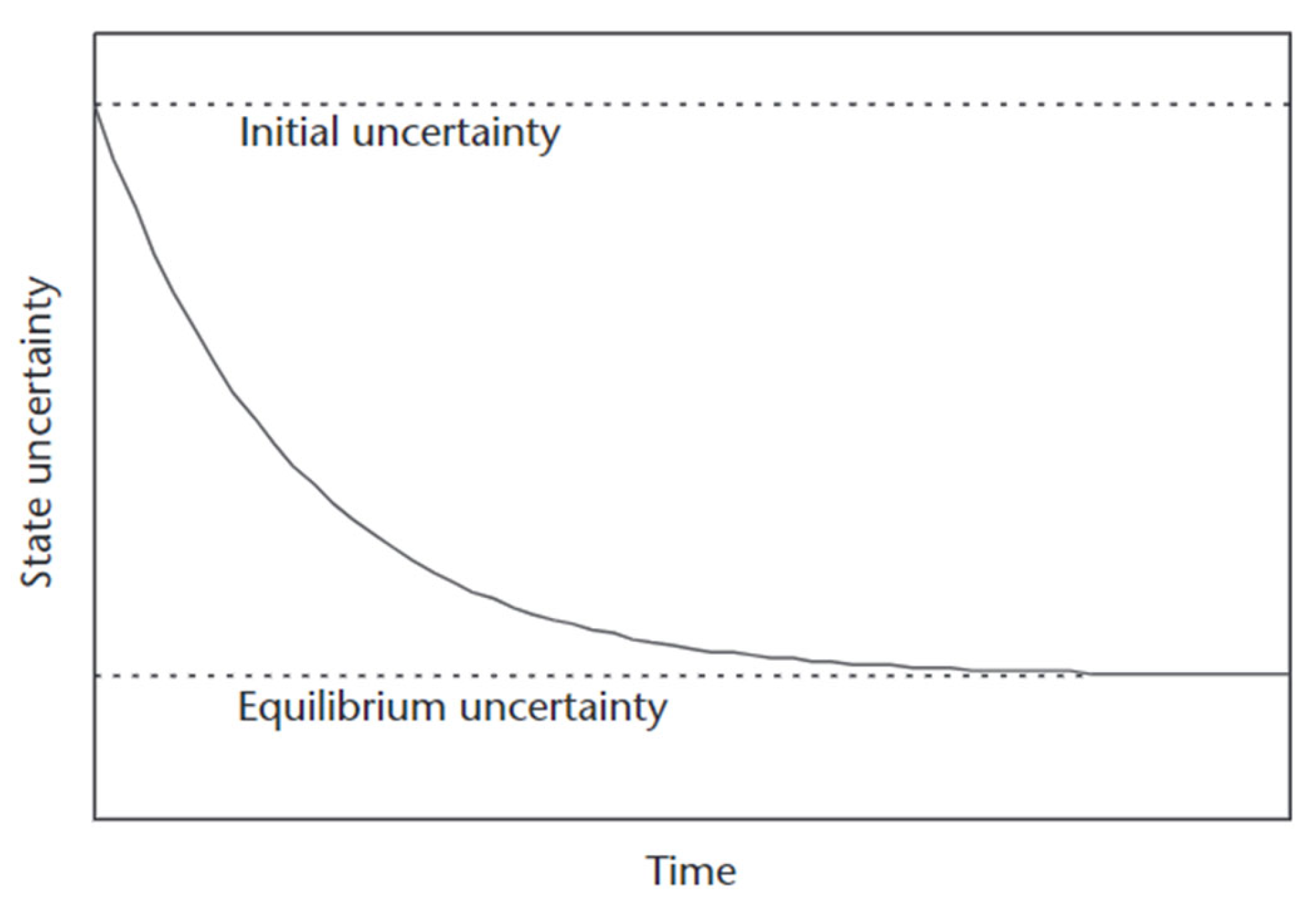
The KF, in a similar way to other filters, needs time to converge and become stable. These values tend to converge to the true values in a fault-free scenario in which correct assumptions are made. This behavior can be observed in the values of the system noise covariance, , which is usually initialized with large values and rapidly converges to stable values (see Figure 1).
The KF performs a combination between the input measured information and the estimated state by means of a weighted sum of these two data sources, in order to avoid poor estimations and observation outliers. This is represented by the Kalman gain matrix, which assigns a measure of trust to the input state and the estimated state; it is computed as follows:
where is the computed Kalman gain matrix, is the measurement matrix, and describes the measurement covariance matrix.
This weighting matrix is applied, as mentioned, as a measure of trust that is given to the measurements and the estimations. This yields:
where is the computed state, is the read measurement vector, and is the innovation vector, which describes the difference between the read measurement and the expected measurement.
Having introduced the KF, and after presenting an overview of its most general form, the particularization of the KF that was employed in this research work is discussed in the following subsection; this leads to the explanation of the sensor fusion approach, known as tightly coupled architecture, and how the integration of the UWB technology is performed.
2.2. Tightly Coupled Sensor Fusion: GNSS, IMU, and UWB
The Kalman filter is a very flexible filter that can be adapted to multiple architectures. This flexibility offers the possibility to modify almost any parameter of the filter, leading to a particular version of itself. When talking about the prediction stage of the filter, for example, two main variations can be found: the total-state KF and the error-state KF.
The former one, on the one hand, can be applied to filters that integrate only positioning systems, but it is also suitable for use with dead reckoning sensors. In this kind of integration, the position solution is predicted forward in time using the velocity solution and, in high-dynamics applications, the acceleration states can also be used to enhance the navigation solution. This type of filter is useful in achieving a smoothing of the noise in the navigation measurements. This kind of prediction can also be used to bridge gaps in the system measurements due to tunnels or other kinds of signal outage-causing objects [26].
The error-state integration, on the other hand, is an integration type in which the navigation solution of a certain reference navigation system is corrected using measurements from the complementary navigation system. The said reference system must be an inertia-measuring device or some kind of [26,27] dead reckoning type of system. The state vector, in this case, is formed by the error states for the reference navigation system, which consist of the attitude, velocity, and position errors, together with the clock bias and drift estimations. Note that in the absence of a relative navigation system (i.e., IMU), the error-state integration converges to the total-state integration.
The design of a filter and, specifically, its integration architecture can be understood as a tradeoff between the optimization of the processing efficiency and the maximization of the robustness and accuracy of the navigation solution. At the time of fusing different types of measurements, the KF offers the possibility of being configured according to different architectures, depending on the stage at which the data are fused; this leads to three common architectures: the loosely coupled KF, the tightly coupled KF, and the deeply coupled KF [26].
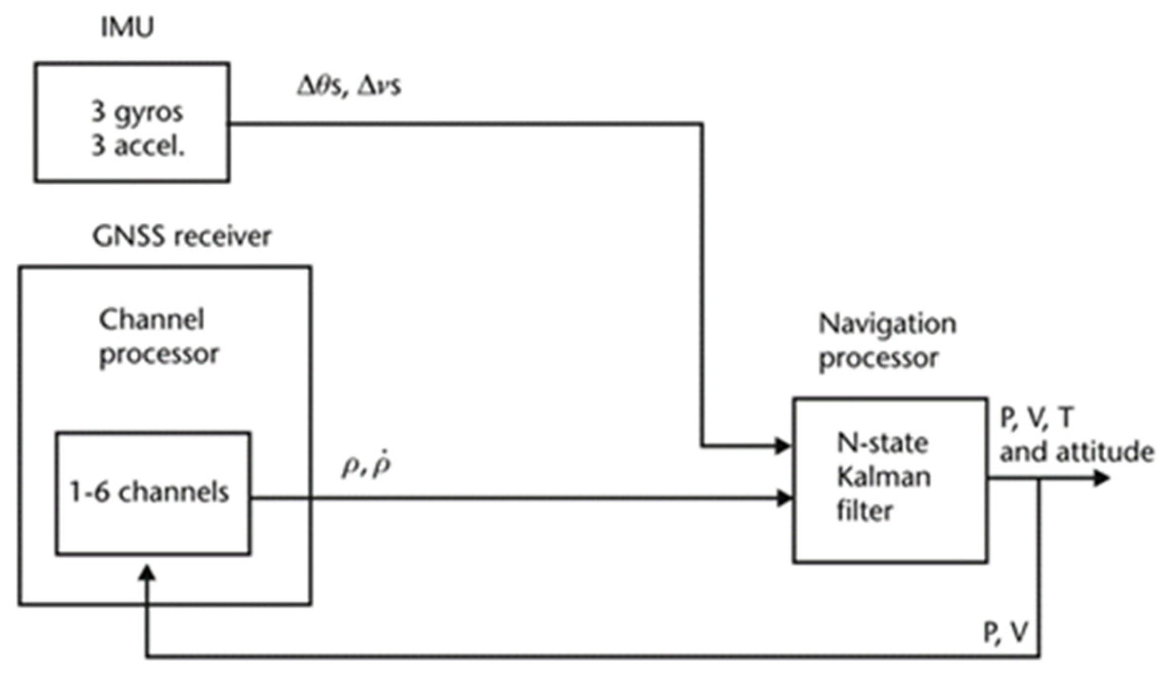
As recently discussed, three commonly used sensor integration architectures can be found when fusing GNSS and IMU data and two main types of prediction stages. In this research work, the tightly coupled integration (see Figure 2 and Figure 3) was employed, which is mainly used in scenarios in which the possibility of having incomplete data is high. In this architecture, raw data from all the sensors are fed to the same KF, and the PVT solutions are no longer used until the final output estimation of the system. Consequently, it is the KF external to the main sensor that is the one in charge of estimating the output state from the input raw data. Moreover, an error-state prediction-based version of the algorithm was chosen in order to fuse the range-based data from GNSS and UWB with the acceleration and gyroscope data provided by the IMU [26,27].
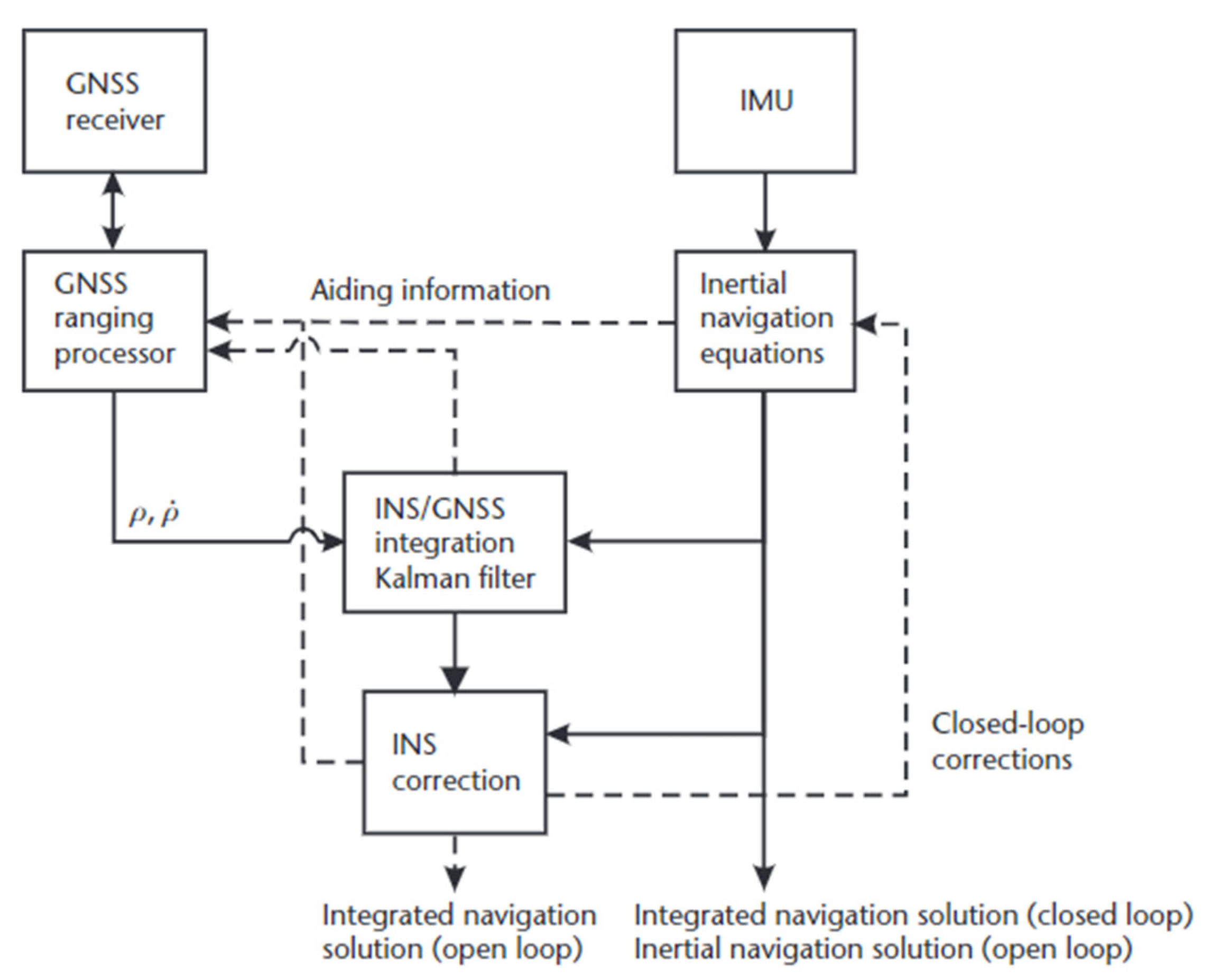
The error-state prediction architecture is a variation of the Kalman filter that does not directly estimate the state vector of the filter but, instead, estimates an error vector of the filter, which is computed by the propagation of the a priori errors and noise power spectral density (PSD) of the measurements. Depending on the architecture of the filter, this can be used to only estimate the error vector, which is also known as an open-loop architecture, or to compute the state vector by applying a closed-loop correction (Figure 3).
Therefore, in an error-state implementation of the Kalman filter, the state vector described in (5) no longer represents the estimation of the filter’s state, but the estimation of the error vector, which models the remaining errors in the system after the correction of the state. This error vector can be represented as follows:
where describe the error uncertainties of the attitude, describe the error uncertainties of the velocity, describe the error uncertainties of the position, describe the error uncertainties of the accelerometer bias, describe the error uncertainties of the gyroscope bias, and describe the clock offset and clock drift uncertainties, accordingly.
This state estimates are usually initialized with zero values, contrary to what is performed in the total-state filters, where an initial-state estimation such as the LSE is performed. This initialized error-state vector should be propagated using a different transition matrix which models the propagation of the error estimation with time. In this research work, the transition matrix shown in [26] was adapted to include position and clock data and to match the state vector shown in (5). Let the employed transition matrix be:
where describes the last computed position; describes the transition interval; are zero and identity matrixes, respectively; denotes the skew-symmetric matrix of Earth rate; is the skew matrix of with being the last measured specific force; describes the gravity force at as , being ; and is the gravity vector and the geocentric radius at .
Accordingly, the system noise covariance matrix, , introduced in (2) is defined as stated in [26]:
where , and are the power spectral densities of, respectively, the gyro random noise, accelerometer random noise, accelerometer bias variation, and gyro bias variation, and it is assumed that all the gyros and all the accelerometers have equal noise characteristics. Note that the matrix proposed in [26] was extended from 15 × 15 to 17 × 17 in order to include the clock phase noise, , and the clock frequency, . Note that these values were obtained from the datasheet of the devices in Table 1, according to the explanations in [26].
The closed-loop architecture implementation allows the achievement of a high performance out of an error-state KF due to the fact that the estimated errors are fed back to the filter every iteration, correcting in this way the system itself and zeroing the filter’s states. Consequently, the filter’s states remain small, minimizing the effect of higher-order products in the system model. Note that the same amount is added to or subtracted from the estimated state and the true state; thus, the error covariance matrix is not affected by the feedback process [26,27].
When trying to fuse different sensor data for navigation, not only does the KF consider the geometry of the input sources, but also the dynamism of the system. As a consequence, a group of commonly based observations such as the range-based observations can be gathered even if they come from different types of sensors (i.e., GNSS, UWB, Bluetooth, etc.). Due to the fact that these measurements model the same physical parameter (i.e., the distance from the receiver’s antenna to the transmitting system’s antenna), they can be indistinctively processed. Accordingly, introducing UWB measurements to the commonly employed GNSS+IMU sensor fusion fulfils the first requirements a priori. For this purpose, the observation matrix, , shown in (8) is shaped as follows:
where represent the normalized vectors linking the GNSS antenna and each of the employed satellites, and represent the normalized vectors linking the UWB antenna and each of the employed transmitting UWB antennae.
Note that the UWB range observables can be linearized analogously to the GNSS pseudo-range observables but avoid the clock drift field, which is not contemplated and, thus, is represented with a null derivative value. Moreover, it should be noted that no lever arm is contemplated since the same reference is employed for both GNSS and UWB antennae, neglecting any possible location error between them. Nevertheless, any other setup should consider said lever arm in order to add said antennae separation.
Moreover, the addition of the UWB ranges to the GNSS observables, due to their similarity, was performed by adding the UWB ranges to the observable vector of the KF, , without the need for any kind of transformation; thus:
where is the pseudo-range measurement for the satellite, is the range measurement for the UWB anchor, and is the doppler measurement for the satellite.
Accordingly, as different sourced measurements are to be fused, this should be reflected in all the parameters of the filter related to the observables. This could vary depending on the design of the filter; however, following the architecture shown in previous sections, the only parameter of the Kalman filter that depends on the number of measurements and their characteristics is the measurement covariance matrix described by . This diagonal matrix is open to characterization, as different approaches can be found in the literature. In this research, the elements were weighted according to the power spectral density (PSD) and then reweighted according to the signal’s signal-to-noise-ratio (SNR) and satellite elevation in the case of the satellite signals and according to the elevation in the case of the UWB signals. The diagonal elements of the matrix that correspond to the satellite signals are characterized as:
The latter term of the equality, which is used for the unequal reweighting of the observables, was modelled as follows [28]:
where , and are empirical design parameters; denotes the elevation of satellite ; and quantifies the SNR of satellite .
The diagonal elements that correspond to the UWB signals, on the other hand, are reweighted by following an adaptation of a previous version of (11) that takes into account the signal’s received signal strength indicator (RSSI) instead of the SNR. This equation is described as:
where denotes the elevation of anchor and is the RSSI of the signal received from anchor .
Note that the RSSI is an estimated measure of the power level of the incoming signal. This parameter becomes smaller at larger distances, which intuitively matches the attenuation behavior of the signals when travelling in space. This indicator, consequently, is used to estimate how well a particular radio receiver will receive data from the transmitting system.
Analogously to GNSS, the RSSI and elevation masks were applied to the UWB measurements, which were tunable by the user according to the needs of the scenario.
When fusing different types of radio-based observables, the proper design of the measurement covariance matrix is a crucial step, as unbalances in the measurement weighting can lead to undesired biases in the result. Following the mentioned case of the fusing of GNSS and UWB signals, since UWB signals offer a lower range of error uncertainty, they have a higher impact on the measurement weighting. This may imply an improvement compared to using just GNSS signals; however, any unexpected error in a UWB signal may degrade the performance of the fusion, regardless of the quality of the GNSS signals.
3. Results
The following section shows and analyzes the real-world scenarios that were used to test the implemented algorithm and the improvement on the addition of UWB technology to the GNSS+IMU sensor fusion, especially for precision approaching and maneuvering. These scenarios gather two of the main motorized transportation domains, such as maritime and automotive and the particular complexities that make them considerably challenging scenarios.
In every test, the setup of the equipment was composed in the following way: the antennae (see Figure 4) were placed on the highest or (when not available) the best visibility point of the vehicle (on the deck of the boat—see Figure 5; in the trunk of the car—see Figure 6), while the corresponding receivers (the commercial off-the-shelf GNSS receiver and the proprietary UWB receiver developed by CEIT-BRTA [29,30]), the reference high-performance positioning system and the recording computer were located in the closest covered and safe part of the vehicle (on the deck of the boat—see Figure 5; in the trunk of the car—see Figure 6), to avoid damage to the devices.
Moreover, the UWB anchors were placed within the limits of the measurement site (Figure 9), to cover all the areas in which the vehicle could go through during its maneuvers. The UWB anchors with good satellite visibility were located with the same high-performance navigation system, applying real-time-kinematics (RTK) corrections to the positioning algorithm, in order to obtain centimeter-level accuracy. If any anchor was located in a low visibility location, it was located by rotating relative to the local X-Y coordinates from known trustworthy coordinates to east–north–up (ENU) coordinates for a later translation to ECEF absolute coordinates.
For the relative location of said anchors, the accurate position of the rest of the anchors was used, as the solutions obtained from the RTK positioning were assumed to be accurate enough. The ground truth, on the other hand, was obtained using the same high-performance system, applying the required corrections to obtain an RTK centimeter-level position.
Between the installed sensors, two main groups should be distinguished. On the one hand, the IMU acts as a device to measure and report the specific forces and angular rates of the car. On the other hand, both GNSS and UWB act as range-based technologies which are used by applying the principle of trilateration. Accordingly, these two radio technologies will suffer similar degradation when lacking the line-of-sight (LOS) component of their signals and when an excessive multipath is found. However, the use case-tailored geometry and location of the UWB anchors allow the avoidance of part of the mentioned signal-degrading effects, making this technology less likely to suffer from this error source.
3.1. Automotive
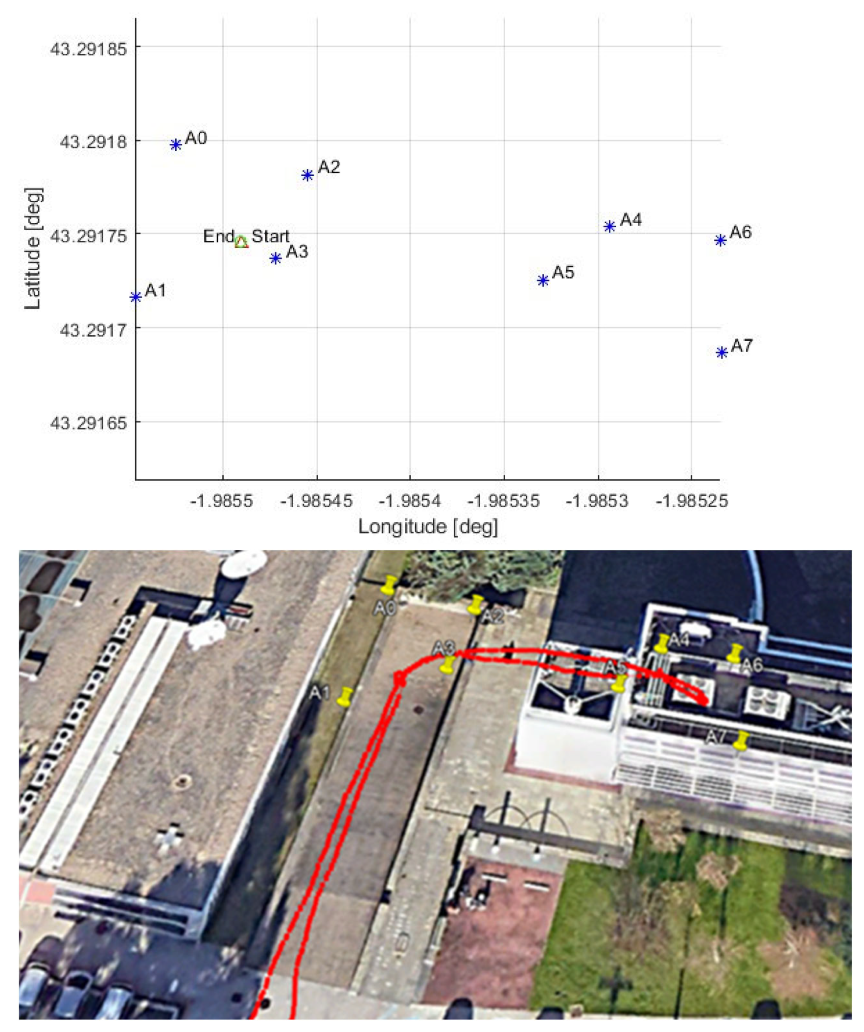
This measurement scenario is located at the technological park of Miramon, San Sebastian, Spain. This suburban site is a suitable environment to check the performance of the enhancement of a GNSS+IMU-based navigation system with the UWB technology since it contains a complex urban canyon composed of a high building density zone followed by an indoor part inside a garage, where abrupt maneuvers were performed to turn the car back to the outside of the garage. This indoor area implies a challenge for the GNSS due to its lack of satellite visibility and for the IMU due to the high accelerations. Accordingly, locating UWB transmitting anchors around and inside said indoor area allows, first, a position accuracy enhancement and then an indoor navigation where no GNSS coverage is found.
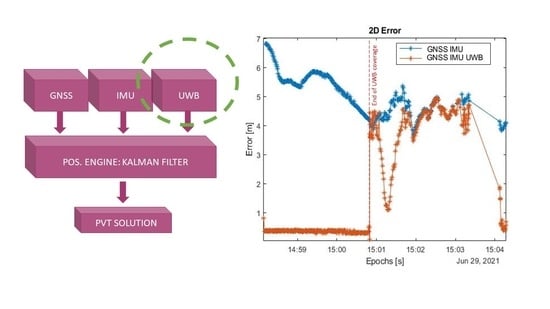
The analyzed measurements belong to the maneuvers performed with a commercial five-seat car inside the UWB signal coverage zone, where the same procedure was repeated for seven consecutive rounds. This procedure is as follows: The car in which the setup was installed begins its operation when located at the convergence spot that can be seen between anchors A0, A1, and A3 in Figure 7 or the start spot in Figure 7. After waiting for approximately 30 s, the car initiates its operation towards the outside of the garage zone (also the UWB signal coverage zone) at 4 m/s, only to maneuver outside and enter again following the same path at the same velocity. Once in front of the garage’s entrance, the car goes inside the indoor environment (close to 40 s without GNSS data available; see Figure 8) until the imaginary edge forms the anchors A6 and A7, after which a reorienting maneuver is performed to finish back at the starting point (start/end spot in Figure 7), where it remains stationary for 15 s and the recording systems are paused.
An example of the representation of said maneuvers can be observed in Figure 8. This figure shows the visibility of each UWB anchor in terms of the coverage range and RSSI when these are read by the moving onboard tag. Accordingly, it can be seen how the ranges correlate with the behavior explained in the previous paragraph: they remain still for approximately 30 s, only to increase their value until the onboard tag decouples from the last visible anchor. After having maneuvered outside of the garage area, the read range values decrease (meaning that the car approaches their location), show a disturbance related to the reorienting maneuver, and remain still for some seconds at the same value as in the beginning, due to the same starting and ending locations of the testing car during the measurement.
The RSSI from the received signals shows a similar behavior; it is bigger at a shorter distance between the transmitter anchors and receiver tag (with values between −79 dBm and −97 dBm) and shows noise of less stable values when a clear LOS signal is not received. Note that due to the fact that RSSI values seem to be noisier from −86 dBm, and become noisier the lower the RSSI value, a RSSI mask has been defined at said −86 dBm.
Note that Figure 8 shows a UWB data gap between 15:01:20 and 15:03:20. This lack of UWB corresponds to the period in which the car goes outside the UWB coverage zone and maneuvers to proceed back inside the UWB coverage zone again. Moreover, it also shows the 40 s period inside the indoor environment in which no GNSS data are available and in which fast UWB range variations can be observed.
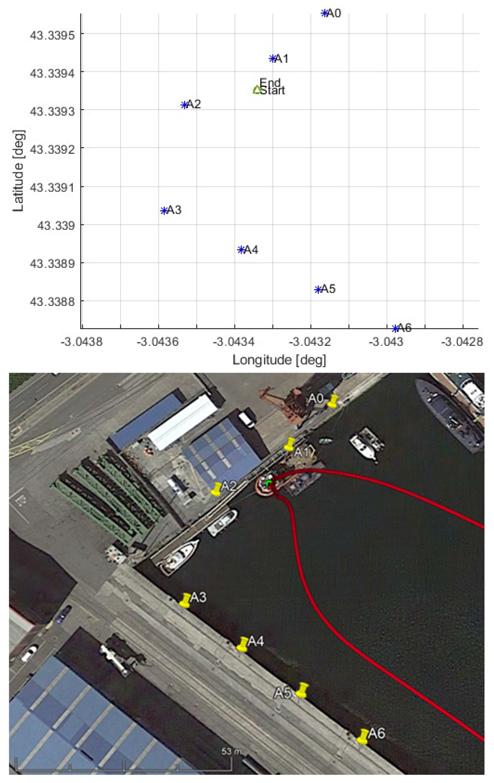
3.2. Maritime
The maritime scenario in which the algorithm was tested is a water inlet in the industrial environment of the port of Bilbao, which is surrounded by ships and metal objects that can affect the reception of both GNSS signals. This real environment was used to carry out docking/undocking maneuvers and to test whether the UWB-based position accuracy enhancement would fulfil the expectations set by the previous automotive scenario, given the open shape of the transmitting anchor location over the port. Moreover, the advantages of employing a tightly coupled algorithm were tested in this scenario. Note that the L-shaped open geometry of the transmitting anchors does not allow the presence of more than three contemporary usable observables continuously. This suboptimal geometry (according to the literature, optimal geometries tend to have closed shapes. See [31,32,33,34,35] for optimal geometry calculations) would generate complexities for a loosely coupled algorithm, since this would require three contemporary signals to compute a position. Nevertheless, the implemented tightly coupled algorithm fuses the available UWB signals (signals with a time difference smaller than 0.3 seg from the GNSS timestamp) with GNSS observables at every GNSS timestamp, allowing the use of even a single UWB signal.
The analyzed measurements belong to the docking/undocking maneuvers of an 18 m long tugboat (provided by the local maritime authorities) that were performed inside the UWB signal coverage zone, where the same procedure was repeated for five consecutive rounds. This procedure is as follows: The ship on which the setup was installed began its operation when located at the convergence spot (green spot) that can be seen between anchors A1 and A2 in Figure 9 or the start spot in Figure 9. After waiting for approximately 60 s, the ship initiated its undocking operation towards the outside of the port (also the UWB signal coverage zone), only to maneuver outside and enter again following an anticlockwise circular path, all at a mean speed of 3 m/s. Once approaching the docking point, the ship started decelerating in order to stop right at the starting spot (start/end spot in Figure 9). Note that the docking maneuver was performed from the side where no UWB anchors were located, leading to a later recoupling with the augmentation system.
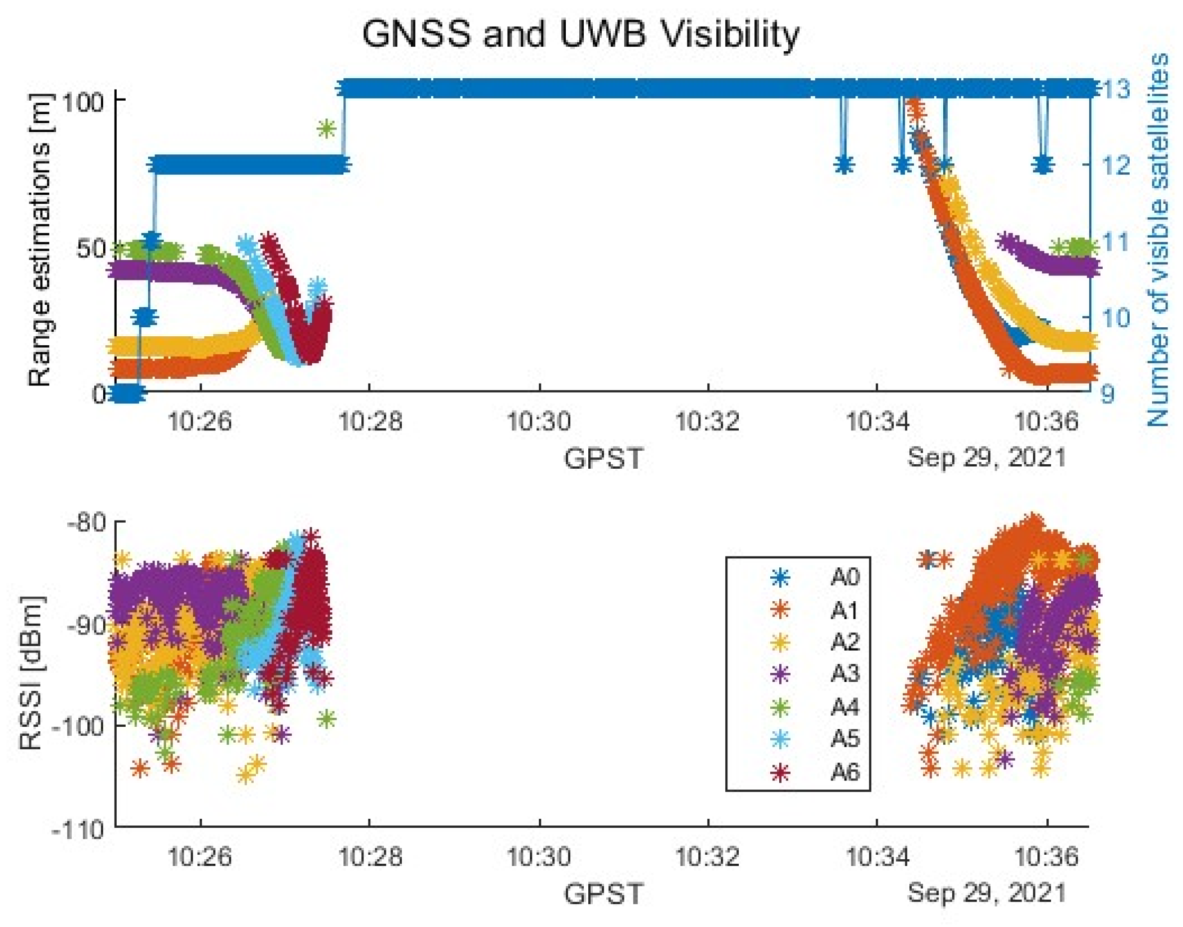
In a similar way to the automotive scenario, an example of the representation of said maneuvers can be observed in Figure 10. This figure shows the visibility of each UWB anchor in terms of the coverage range and RSSI when these are read by the moving onboard tag. Accordingly, it can be seen how the ranges correlate with the behavior explained in the previous paragraph: they remain still for approximately 30 s, only to increase their value until the onboard tag decouples from the last visible anchor. After having undocked, while performing the docking maneuver, the read range values decrease (meaning that the car approaches their location), show a disturbance related to the reorienting maneuver, and remain still for some seconds at the same value as in the beginning, due to the same starting and ending locations of the testing car during the measurement.
The RSSI from the received signals again shows a similar behavior; it is bigger at a shorter distance between the transmitter anchors and receiver tag (with values between −80 dBm and −106 dBm) and seems to be noisier at smaller values. In this case, the same −86 dBm RSSI mask was employed in order to compute the results shown in the next section.
Note that Figure 10 shows (analogously to Figure 8) a UWB data gap between 10:27:32 and 10:34:19. This lack of UWB corresponds to the period between the undocking and the docking of the boat, in which the boat goes outside the UWB coverage zone and maneuvers to proceed back inside the UWB coverage zone again. Moreover, it can also be observed that, since this scenario offers a constant LOS component of every UWB signal, the measured ranges are significantly higher than in the previous scenario. However, this increase in range implies a significant reduction in the RSSI, decreasing its a priori reliability.
4. Discussion
This section shows and analyzes the results obtained when applying the implemented UWB-based augmentation to the GNSS+IMU tightly coupled Kalman filter. These results were obtained after processing the data collected in the measurements explained in Section 3. It should be noted that the computation of the performance of this sensor fusion approach was limited to the coverage region of the UWB transmitting anchors, which were deployed only where precision maneuvering was needed. Not only was this carried out due to the available resources, but because of the economical limitation of this approach. Even though the performance of this technological approach significantly outperforms the GNSS+IMU fusion in terms of accuracy and overall availability, the cost increases proportionally to the number of anchors to be deployed. Accordingly, since commercial off-the-shelf UWB systems provide a limited coverage outdoors (<30 m of radius), the cost increase of deploying UWB anchors all over the vehicle’s route would make this approach unsuitable for some applications. Moreover, the accurate absolute positioning of each anchor may become a time-consuming task, which would significantly increase the cost if the UWB anchors were deployed all over the vehicle’s route.
The computation of the error was performed by comparing the calculated solution’s position with the ground truth’s coordinates with the closest time value. As the output data rate of this ground truth was ten times higher than the one of the developed navigation algorithm, a maximum time error of 0.1 s could be suffered and, thus, added to the computed error.
The tables in the following subsections summarize the results of the multiple measurement rounds performed in the test sites described in Section 3. The first table in every set evaluates each of the performed rounds in terms of the horizontal error, which is divided into the minimum, mean, and maximum values, together with its variance and 95th percentile. Moreover, the second table of every set shows the improvement ratio introduced by the UWB-based augmentation.
4.1. Automotive
The following Table 2 shows the improvement introduced when applying UWB technology as an augmentation system to be used during precision approaching or maneuvers in the automotive domain, and its comparison with the performance of a navigation system is based only on a low-cost GNSS receiver and a low-cost IMU. As mentioned, these measurements consist of seven consecutive rounds to ensure repeatability. Due to the fact that this scenario includes an indoor environment with no GNSS signal coverage (see Figure 8), the indoor maneuvering is based on the dead reckoning of the IMU for the GNSS+IMU approach and a tightly coupled UWB+IMU for the UWB-augmented approach.
For the sake of an easier understanding, the discussion on the results is mainly presented in the second table (Table 2), which shows the improvement of the GNSS+IMU+UWB system against the GNSS+IMU one. This table provides an easier way of understanding the results since it shows the ratio between the postprocessed results round by round and uses a color coding that emphasizes the observed phenomenon. Accordingly, a green cell denotes a reduction in the horizontal positioning error (HPE), a red cell denotes an increase in the HPE, and the colorless cell denotes no change in the HPE. Note that every value in the “# solutions” column shows no variation from the introduction of UWB technology since there was no epoch without GNSS coverage that required more observables to be able to compute a solution.
Accordingly, by checking the color code (Table 2), at a first glance the reduction in the HPE is obvious since every cell shows a reduction except for that from round 6, where an increase in the maximum error can be observed. Nevertheless, this increase in the peak maximum error comes with a reduction in the 95th percentile error and a reduction in the variance, which implies an overall reduction in the distance of the highest error values from the mean. The lowest value remains unchanged at 3.87 m.
Moreover, going into the numerical values, a significant reduction in the HPE can be observed, up to 96% of the mean, and even 100% (rounded periodic decimal of 99.9%). This significant reduction represents an order of magnitude reduction in 5 out of 7 rounds, reaching a submeter accuracy; and an accuracy of almost below 50 cm in 4 out of 7 rounds (rounds 1 to 4). In this way, the introduction of UWB as an augmentation system caused an overall significant reduction in the HPE and helped avoid the long dead reckoning stage of the IMU inside the GNSS signal-lacking zone (inside the garage). Note that this dead reckoning of the IMU, even if it generates a continuous stream of solutions where there are no GNSS data available, accumulates an error that increases with time until new ranging data are received.
4.2. Maritime
The following tables show the improvement introduced when applying UWB technology with suboptimal geometry as an augmentation system to be used during precision approaching or maneuvers in the maritime domain, and its comparison with the performance of a navigation system is based only on a low-cost GNSS receiver and a low-cost IMU. As mentioned, these measurements are composed of five consecutive rounds in order to be able to draw meaningful conclusions.
Note that the previously described criterion for understanding the table is still valid for the above in Table 3. Accordingly, a green cell denotes a reduction in the horizontal positioning Error (HPE), a red cell denotes an increase in the HPE, and a colorless cell denotes no change in the HPE. Analogously to what is seen in Table 2, it can be seen that every value in the “# solutions” column shows no variation from the introduction of UWB technology, since there was no epoch without GNSS coverage that required more observables to be able to compute a solution (see Figure 10).
Regarding the accuracy, an improvement of 51–98% can be observed in the minimum HPE which, together with the improvement of the maximum HPE of up to 52%, causes an improvement of the mean HPE up to 88% (Table 3). Note that the reduction in the mean HPE may imply a reduction in the overall accuracy of the solution, but when this reduction is added to the reduction in the error variance, it can be concluded that not only were the error peaks reduced, but also the overall distribution of the error, which led to a higher convergence of the error towards the ground truth.
5. Conclusions
This paper confirmed the suitability of UWB observables as an augmentation system for a GNSS+IMU-based navigation system that can be used for precision approaching or maneuvering. Accordingly, the feasibility of said sensor fusion was proven and discussed, as a continuation of the work found in the literature mentioned in the introduction.
Moreover, this sensor fusion was tested in a dynamically changing real-world scenarios, proving not only that the proposed GNSS+IMU+UWB algorithm works and is valid for everyday use, but also that it significantly improves the commonly employed GNSS+IMU algorithm when employed with low-cost systems in challenging scenarios. This improvement becomes clear in the results shown in the tables in Section 4, where the mean reduction in the HPE reaches 72% for the automotive domain and 80% for the maritime domain. Furthermore, the employed fusion allowed submeter accuracy to be reached for five out of seven measurements in the automotive domain and three out of five measurements in the maritime domain.
Furthermore, two different UWB anchor geometries were tested in the mentioned real-life environments: an open geometry one and a closed one. Even though the studies in literature show that the optimal placement of transmitting UWB anchors is a closed shape for standalone UWB positioning, when this is employed as an augmentation system for another ranging technology such as GNSS, a suboptimal open UWB anchor geometry is still valid when observing improvements in the solution’s accuracy.
In conclusion, the implemented sensor fusion allowed the achievement of a decrease of an order of magnitude with respect to the one provided by low-cost GNSS+IMU commercial systems, regardless of the means of transport or the scenario.
Further research will explore, on the one hand, the use of the proposed sensor fusion for other transportation domains, such as the railway. On the other hand, the possibility of employing other low-cost sensors to improve the capabilities of navigation systems will be explored. Afterwards, having ensured improvements in accuracy and continuity, the integrity aspect of this (or future) multisensor approach will be studied. In this context, the definition of tailored protection levels will be carried out. For this purpose, individual and common approaches will be studied for the different means of transport.
Author Contributions
Conceptualization, P.Z. and G.D.M.; methodology, P.Z. and G.D.M.; software, P.Z.; validation, P.Z. and G.D.M.; investigation, P.Z. and G.D.M.; data curation, N.F.-B. and J.A.; writing—original draft preparation, P.Z.; writing—review and editing, G.D.M., N.F.-B., J.A., I.A. and J.M.; visualization, N.F.-B. and J.A.; supervision, I.A. and J.M.; project administration, I.A. and J.M.; funding acquisition, I.A. and J.M. All authors have read and agreed to the published version of the manuscript.
Funding
This research was funded by HORIZON 2020 X2RAIL-5, grant number 101014520.
Data Availability Statement
Data are contained within the article.
Conflicts of Interest
The authors declare no conflicts of interest.
References
- Novak, A.; Skultety, F.; Bugaj, M.; Jun, F. Safety Studies on GNSS Instrument Approach at Žilina Airport. In Proceedings of the MOSATT 2019—Modern Safety Technologies in Transportation International Scientific Conference, Piscataway, NJ, USA, 28–29 November 2019; Institute of Electrical and Electronics Engineers Inc.: Piscataway, NJ, USA, 2019; pp. 122–125. [Google Scholar] [CrossRef]
- Manz, H. Safety relevant application of satellite based localisation in transportation with the focus on railways. In Proceedings of the 2015 International Association of Institutes of Navigation World Congress, IAIN 2015, Prague, Czech Republic, 20–23 October 2015; Institute of Electrical and Electronics Engineers Inc.: Piscataway, NJ, USA, 2015. [Google Scholar] [CrossRef]
- Zhang, Q.; Niu, X.; Shi, C. Impact Assessment of Various IMU Error Sources on the Relative Accuracy of the GNSS/INS Systems. IEEE Sens. J. 2020, 20, 5026–5038. [Google Scholar] [CrossRef]
- Amami, M.; Amami, M.M. The Advantages and Limitations of Low-Cost Single Frequency GPS/MEMS-Based INS Integration. Glob. J. Eng. Technol. Adv. 2022, 2022, 018–031. [Google Scholar] [CrossRef]
- Groves, P.D.; Wang, L.; Walter, D.; Martin, H.; Voutsis, K.; Jiang, Z. The four key challenges of advanced multisensor navigation and positioning. In Record—IEEE PLANS, Position Location and Navigation Symposium; IEEE: Piscataway, NJ, USA, 2014; pp. 773–792. [Google Scholar] [CrossRef]
- Grejner-Brzezinska, D.A.; Toth, C.K.; Moore, T.; Raquet, J.F.; Miller, M.M.; Kealy, A. Multisensor Navigation Systems: A Remedy for GNSS Vulnerabilities? Proc. IEEE 2016, 104, 1339–1353. [Google Scholar] [CrossRef]
- Ubisense—Ultra-Wideband Real-Time Location System (RTLS). Available online: https://ubisense.com/ (accessed on 30 November 2020).
- Lee, Y.; Kim, J.; Lee, H.; Moon, K. IoT-based data transmitting system using a UWB and RFID system in smart warehouse. In Proceedings of the International Conference on Ubiquitous and Future Networks, ICUFN, Milan, Italy, 4–7 July 2017; IEEE Computer Society: Washington, DC, USA, 2017; pp. 545–547. [Google Scholar] [CrossRef]
- Pochanin, G. Application of the Industry 4.0 Paradigm to the Design of a UWB Radiolocation System for Humanitarian Demining. In Proceedings of the UWBUSIS 2018—2018 9th International Conference on Ultrawideband and Ultrashort Impulse Signals, Odessa, Ukraine, 4–7 September 2018; Institute of Electrical and Electronics Engineers Inc.: Piscataway, NJ, USA, 2018; pp. 50–56. [Google Scholar] [CrossRef]
- Gao, Y.; Meng, X.; Hancock, C.M.; Stephenson, S.; Zhang, Q. UWB/GNSS-based Cooperative Positioning Method for V2X Applications. 2014. Available online: https://nottingham-repository.worktribe.com/output/733331 (accessed on 30 September 2020).
- Cheng, L.; Chang, H.; Wang, K.; Wu, Z. Real Time Indoor Positioning System for Smart Grid based on UWB and Artificial Intelligence Techniques. In Proceedings of the 2020 IEEE Conference on Technologies for Sustainability, Oklahoma City, OK, USA, 2020; SusTech: Shenzhen, China, 2020. [Google Scholar] [CrossRef]
- Corrales, J.A.; Candelas, F.A.; Torres, F. Hybrid tracking of human operators using IMU/UWB data fusion by a Kalman filte. In Proceedings of the HRI 2008—3rd ACM/IEEE International Conference on Human-Robot Interaction: Living with Robots, Amsterdam, The Netherlands, 12–15 March 2008; pp. 193–200. [Google Scholar] [CrossRef]
- Tiemann, J.; Schweikowski, F.; Wietfeld, C. Design of an UWB indoor-positioning system for UAV navigation in GNSS-denied environments. In Proceedings of the 2015 International Conference on Indoor Positioning and Indoor Navigation, IPIN 2015, Banff, AB, Canada, 13–16 October 2015. [Google Scholar] [CrossRef]
- Macgougan, G.; O’Keefe, K.; Klukas, R. Tightly-coupled GPS/UWB positioning: First test results from a difficult urban environment. In Proceedings of the 2009 IEEE International Conference on Ultra-Wideband, ICUWB 2009, Vancouver, BC, Canada, 9–11 September 2009; pp. 381–385. [Google Scholar] [CrossRef]
- MacGougan, G.; O’Keefe, K.; Klukas, R. Accuracy and reliability of tightly coupled GPS/ultra-wideband positioning for surveying in urban environments. GPS Solut. 2010, 14, 351–364. [Google Scholar] [CrossRef]
- MacGougan, G.; O’Keefe, K.; Chiu, D.S. Multiple UWB Range Assisted GPS RTK in Hostile Environments. In Proceedings of the 21st International Technical Meeting of the Satellite Division of The Institute of Navigation (ION GNSS 2008), Savannah, Georgia, 16–19 September 2008; Available online: https://www.ion.org/publications/abstract.cfm?articleID=8208 (accessed on 30 January 2024).
- Zhang, R.G.; Shen, F.; Li, Q.H. A Hybrid Indoor/Outdoor Positioning and Orientation Solution Based on INS, UWB and Dual-Antenna RTK-GNSS. In Proceedings of the 27th Saint Petersburg International Conference on Integrated Navigation Systems, ICINS 2020—Proceedings, St. Petersburg, Russia, 25–27 May 2020. [Google Scholar] [CrossRef]
- Di Pietra, V.; Dabove, P.; Piras, M. Loosely Coupled GNSS and UWB with INS Integration for Indoor/Outdoor Pedestrian Navigation. Sensors 2020, 20, 6292. [Google Scholar] [CrossRef]
- Li, Z.; Chang, G.; Gao, J.; Wang, J. Hernandez. GPS/UWB/MEMS-IMU tightly coupled navigation with improved robust Kalman filter. Adv. Space Res. 2016, 58, 2424–2434. [Google Scholar] [CrossRef]
- Wang, C.; Xu, A.; Sui, X.; Hao, Y.; Shi, Z.; Chen, Z. A seamless navigation system and applications for autonomous vehicles using a tightly coupled GNSS/UWB/INS/map integration scheme. Remote Sens. 2022, 14, 27. [Google Scholar] [CrossRef]
- Li, Z.; Wang, R.; Gao, J.; Wang, J. An Approach to Improve the Positioning Performance of GPS/INS/UWB Integrated System with Two-Step Filter. Remote Sens. 2017, 10, 19. [Google Scholar] [CrossRef]
- Zhang, R.; Shen, F.; Liang, Y.; Zhao, D. Using UWB Aided GNSS/INS Integrated Navigation to Bridge GNSS Outages Based on Optimal Anchor Distribution Strategy. In Proceedings of the 2020 IEEE/ION Position, Location and Navigation Symposium, PLANS 2020, Portland, OR, USA, 20–23 April 2020; pp. 1405–1411. [Google Scholar] [CrossRef]
- Jiménez, F.; Naranjo, J.E.; García, F.; Armingol, J.M. Can Low-Cost Road Vehicles Positioning Systems Fulfil Accuracy Specifications of New ADAS Applications? J. Navig. 2011, 64, 251–264. [Google Scholar] [CrossRef]
- I.M.O. (IMO). Resolution A.915(22) Adopted on 29 November 2001 (Agenda item 9) Revised Maritime Policy and Requirements for a Future Global Navigation Satellite System (GNSS); IMO: London, UK, 2001. [Google Scholar]
- European Comission. White Paper on Transport Roadmap to A Single European Transport Area-towards A Competitive and Resource-Efficient Transport System; Publications Office of the European Union: Luxembourg, 2011. [Google Scholar] [CrossRef]
- Groves, P.D. Principles of GNSS, Inertial, and Multisensor Integrated; Artech House: Boston, MA, USA, 2008. [Google Scholar]
- Kaplan, E.; Hegarty, C. Understanding GPS/GNSS: Principles and Applications, 3rd ed.; Artech: Morristown, NJ, USA, 2017; ISBN 9781630814427. [Google Scholar]
- Herrera, A.M.; Suhandri, H.F.; Realini, E.; Reguzzoni, M.; de Lacy, M.C. goGPS: Open-source MATLAB software. GPS Solut. 2016, 20, 595–603. [Google Scholar] [CrossRef]
- Losada, M.; Zamora-Cadenas, L.; Jiménez-Irastorza, A.; Arrue, N.; Vélez, I. UWB-based time-of-arrival ranging system for multipath indoor environments. In Proceedings of the 3rd International Conference on Advances in Circuits, Electronics and Micro-Electronics, CENICS 2010, Venice, Italy, 18–25 July 2010; pp. 17–22. [Google Scholar] [CrossRef]
- Arrue, N.; Losada, M.; Zamora-Cadenas, L.; Jiménez-Irastorza, A.; Vélez, I. Design of an IR-UWB indoor localization system based on a novel RTT ranging estimator. In Proceedings of the 1st International Conference on Sensor Device Technologies and Applications, SENSORDEVICES 2010, Venice, Italy, 18–25 July 2010; pp. 52–57. [Google Scholar] [CrossRef]
- Monica, S.; Ferrari, G. UWB-based localization in large indoor scenarios: Optimized placement of anchor nodes. IEEE Trans. Aerosp. Electron. Syst. 2015, 51, 987–999. [Google Scholar] [CrossRef]
- Chen, Y.Y.; Huang, S.P.; Wu, T.W.; Tsai, W.T.; Liou, C.Y.; Mao, S.G. UWB System for Indoor Positioning and Tracking with Arbitrary Target Orientation, Optimal Anchor Location, and Adaptive NLOS Mitigation. IEEE Trans. Veh. Technol. 2020, 69, 9304–9314. [Google Scholar] [CrossRef]
- Ferrigno, L.; Miele, G.; Milano, F.; Pingerna, V.; Cerro, G.; Laracca, M. A UWB-based localization system: Analysis of the effect of anchor positions and robustness enhancement in indoor environments. In Proceedings of the Conference Record—IEEE Instrumentation and Measurement Technology Conference, Glasgow, UK, 17–20 May 2021; IEEE: Piscataway, NJ, USA, 2021. [Google Scholar] [CrossRef]
- Suwatthikul, C.; Chantaweesomboon, W.; Manatrinon, S.; Athikulwongse, K.; Kaemarungsi, K. Implication of anchor placement on performance of UWB real-time locating system. In Proceedings of the 2017 8th International Conference on Information and Communication Technology for Embedded Systems, IC-ICTES 2017, Chonburi, Thailand, 7–9 May 2017. [Google Scholar] [CrossRef]
- Cerro, G.; Ferrigno, L.; Laracca, M.; Miele, G.; Milano, F.; Pingerna, V. UWB-Based Indoor Localization: How to Optimally Design the Operating Setup? IEEE Trans. Instrum. Meas. 2022, 71, 1–12. [Google Scholar] [CrossRef]
- European GNSS Agency (GSA). Report on Maritime and Inland Waterways User Needs and Requirements. 2018. Available online: https://www.gsc-europa.eu/system/files/galileo_documents/Maritime-Report-on-User-Needs-and-Requirements-v1.0.pdf (accessed on 31 September 2022).
Figure 1.
Kalman filter state uncertainty convergence process [26].
Figure 1.
Kalman filter state uncertainty convergence process [26].

Figure 2.
High–level view of a tightly coupled architecture based on a GNSS+IMU system [26].
Figure 2.
High–level view of a tightly coupled architecture based on a GNSS+IMU system [26].

Figure 3.
Lower-view tightly coupled INS/GNSS integration architecture with open- and closed-loop variations [26].
Figure 3.
Lower-view tightly coupled INS/GNSS integration architecture with open- and closed-loop variations [26].

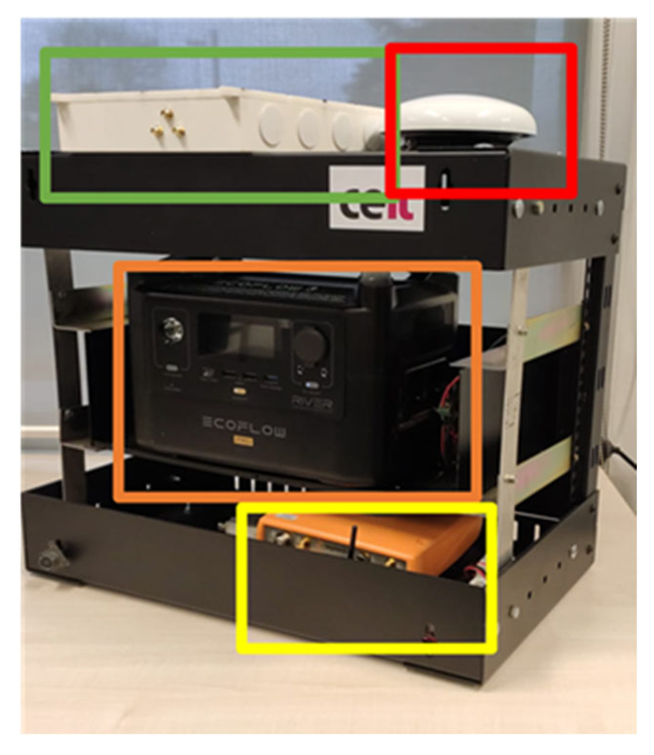
Figure 4.
Employed measurement system (Red: GNSS antenna. Green: navigation system. Orange: power supply. Yellow: ground truth generating system).
Figure 4.
Employed measurement system (Red: GNSS antenna. Green: navigation system. Orange: power supply. Yellow: ground truth generating system).

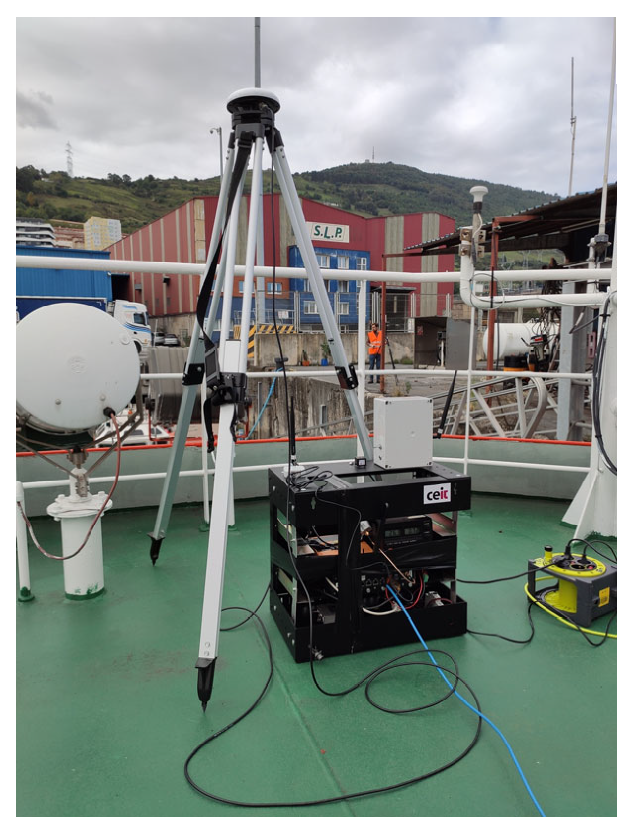
Figure 5.
Onboard measurement setup for the maritime measurement campaign.

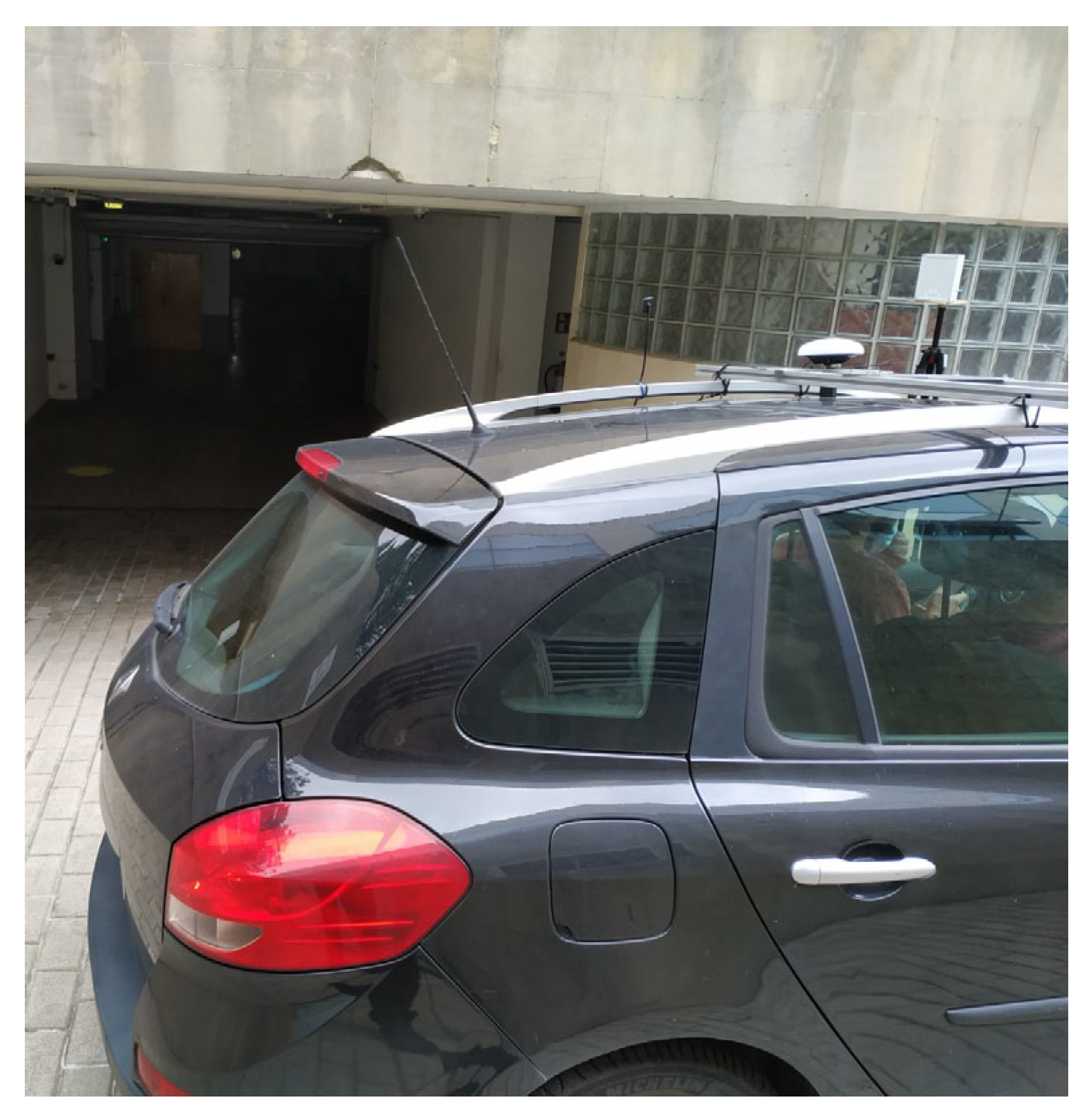
Figure 6.
Onboard measurement setup for the automotive measurement campaign.

Figure 7.
Test scenario: low visibility and indoor areas. Closed-shape distribution of the UWB anchors within the area. (Upper) Location of the anchors relative to the start/end position. (Lower) Location of the anchors and the ground truth in the test scenario.
Figure 7.
Test scenario: low visibility and indoor areas. Closed-shape distribution of the UWB anchors within the area. (Upper) Location of the anchors relative to the start/end position. (Lower) Location of the anchors and the ground truth in the test scenario.

Figure 8.
Example of the visibility of UWB anchors in the automotive measurement.

Figure 9.
Test scenario: suburban environment with surrounding metallic objects and buildings. L-shaped distribution of the UWB anchors within the area. (Upper) Location of the anchors relative to the start/end position. (Lower) Location of the anchors and the ground truth in the test scenario.
Figure 9.
Test scenario: suburban environment with surrounding metallic objects and buildings. L-shaped distribution of the UWB anchors within the area. (Upper) Location of the anchors relative to the start/end position. (Lower) Location of the anchors and the ground truth in the test scenario.

Figure 10.
Example of the visibility of UWB anchors in the maritime measurement.


Table 1.
List of the subsystems in the measurement system.
| Subsystem | Model and Specifications |
|---|---|
| GNSS antenna | Septentrio—PolaNt-x (triple frequency, multi-constellation) (Leuven, Belgium) |
| Low-cost GNSS receiver | Ublox—ZED-F9P mPCIE (dual frequency, multi-constellation) (Thalwil, Switzerland) |
| Low-cost IMU | Advanced Navigation—Orientus (Sydney, Australia) |
| Low-cost UWB receiver | Proprietary hardware |
| Reference system | Septentrio—AsteRx Full (triple frequency, multi-constellation) (Leuven, Belgium) |
| Processing unit | Novatronic—VBox 3611 4L i5-6300U/8 GB RA (Madrid, Spain) |
Table 2.
Horizontal positioning error obtained from the automotive test campaign. (Upper) Absolute results; (Lower) improvement due to the introduction of UWB technology.
Table 2.
Horizontal positioning error obtained from the automotive test campaign. (Upper) Absolute results; (Lower) improvement due to the introduction of UWB technology.
| Scenario Name | Horizontal Error (HPE) [m] | # of Solutions | ||||
|---|---|---|---|---|---|---|
| Min. | Mean | Max. | Variance | 95% | ||
| GNSS_IMU—Round 1 | 3.29 | 7.4 | 10.6 | 0.98 | 8.48 | 328 |
| GNSS_IMU_UWB—Round 1 | 0.26 | 0.3 | 0.51 | 0.05 | 0.34 | 328 |
| GNSS_IMU—Round 2 | 6.32 | 6.66 | 7.5 | 0.09 | 7.33 | 61 |
| GNSS_IMU_UWB—Round 2 | 0.29 | 0.33 | 0.56 | 0.002 | 0.45 | 61 |
| GNSS_IMU—Round 3 | 3.24 | 5.88 | 8.71 | 0.8 | 7.58 | 308 |
| GNSS_IMU_UWB—Round 3 | 0.26 | 0.43 | 0.52 | 0.003 | 0.47 | 308 |
| GNSS_IMU—Round 4 | 3.95 | 6.01 | 7.52 | 0.62 | 7.31 | 219 |
| GNSS_IMU_UWB—Round 4 | 0.24 | 0.27 | 0.39 | 0.0004 | 0.3 | 219 |
| GNSS_IMU—Round 5 | 3.4 | 5.91 | 10.39 | 1.84 | 8.87 | 435 |
| GNSS_IMU_UWB— Round 5 | 0.27 | 0.36 | 0.8 | 0.001 | 0.39 | 435 |
| GNSS_IMU—Round 6 | 3.87 | 5.37 | 7.06 | 0.56 | 6.8 | 213 |
| GNSS_IMU_UWB—Round 6 | 3.87 | 4.7 | 8.2 | 0.3 | 5.49 | 213 |
| GNSS_IMU—Round 7 | 4.35 | 7.74 | 16.7 | 8.22 | 12.34 | 106 |
| GNSS_IMU_UWB—Round 7 | 0.39 | 1.56 | 1.93 | 0.11 | 1.81 | 106 |
| Improvement due to UWB | Horizontal Error (HPE) [m] | # of solutions | ||||
| Min. | Mean | Max. | Variance | 95% | ||
| Round 1 | 92% | 96% | 95% | 95% | 96% | 0% |
| Round 2 | 95% | 95% | 93% | 98% | 94% | 0% |
| Round 3 | 92% | 93% | 94% | 100% | 94% | 0% |
| Round 4 | 94% | 96% | 95% | 100% | 96% | 0% |
| Round 5 | 92% | 94% | 92% | 100% | 96% | 0% |
| Round 6 | 0% | 12% | −16% | 46% | 19% | 0% |
| Round 7 | 91% | 80% | 88% | 99% | 85% | 0% |
Table 3.
Horizontal positioning error obtained from the maritime test campaign. (Upper) Absolute results; (Lower) improvement due to the introduction of UWB technology.
Table 3.
Horizontal positioning error obtained from the maritime test campaign. (Upper) Absolute results; (Lower) improvement due to the introduction of UWB technology.
| Scenario Name | Horizontal Error (HPE) [m] | # of Solutions | ||||
|---|---|---|---|---|---|---|
| Min. | Mean | Max. | Variance | 95% | ||
| GNSS_IMU—Round 1 | 1.82 | 11.11 | 13.76 | 8.46 | 13.53 | 1090 |
| GNSS_IMU_UWB—Round 1 | 0.05 | 3.22 | 6.58 | 4.5 | 6.22 | 1090 |
| GNSS_IMU—Round 2 | 6.9 | 8.02 | 10.99 | 0.79 | 10.09 | 999 |
| GNSS_IMU_UWB—Round 2 | 0.14 | 0.97 | 7.57 | 0.78 | 2.12 | 999 |
| GNSS_IMU—Round 3 | 1.76 | 3.3 | 8.79 | 2.97 | 7.51 | 699 |
| GNSS_IMU_UWB—Round 3 | 0.21 | 1.11 | 6.62 | 0.39 | 1.73 | 699 |
| GNSS_IMU—Round 4 | 0.35 | 1.9 | 4.25 | 0.66 | 3.63 | 1094 |
| GNSS_IMU_UWB—Round 4 | 0.17 | 0.68 | 4.25 | 0.14 | 1.23 | 1094 |
| GNSS_IMU—Round 5 | 0.37 | 2.47 | 4.31 | 0.33 | 3.36 | 3998 |
| GNSS_IMU_UWB—Round 5 | 0.03 | 0.67 | 3.69 | 0.1 | 1.08 | 3998 |
| Improvement Due to UWB | Horizontal Error (HPE) [m] | # of Solutions | ||||
| Min. | Mean | Max. | Variance | 95% | ||
| Round 1 | 97% | 71% | 52% | 47% | 54% | 0% |
| Round 2 | 98% | 88% | 31% | 1% | 79% | 0% |
| Round 3 | 88% | 66% | 25% | 87% | 77% | 0% |
| Round 4 | 51% | 64% | 0% | 79% | 66% | 0% |
| Round 5 | 93% | 73% | 14% | 70% | 68% | 0% |
Disclaimer/Publisher’s Note: The statements, opinions and data contained in all publications are solely those of the individual author(s) and contributor(s) and not of MDPI and/or the editor(s). MDPI and/or the editor(s) disclaim responsibility for any injury to people or property resulting from any ideas, methods, instructions or products referred to in the content. |
© 2024 by the authors. Licensee MDPI, Basel, Switzerland. This article is an open access article distributed under the terms and conditions of the Creative Commons Attribution (CC BY) license (https://creativecommons.org/licenses/by/4.0/).
Share and Cite
MDPI and ACS Style
Zabalegui, P.; De Miguel, G.; Fernández-Berrueta, N.; Aizpuru, J.; Mendizabal, J.; Adín, I. On the Use of Ultra-WideBand-Based Augmentation for Precision Maneuvering. Remote Sens. 2024, 16, 911. https://doi.org/10.3390/rs16050911
AMA Style
Zabalegui P, De Miguel G, Fernández-Berrueta N, Aizpuru J, Mendizabal J, Adín I. On the Use of Ultra-WideBand-Based Augmentation for Precision Maneuvering. Remote Sensing. 2024; 16(5):911. https://doi.org/10.3390/rs16050911
Chicago/Turabian StyleZabalegui, Paul, Gorka De Miguel, Nerea Fernández-Berrueta, Joanes Aizpuru, Jaizki Mendizabal, and Iñigo Adín. 2024. "On the Use of Ultra-WideBand-Based Augmentation for Precision Maneuvering" Remote Sensing 16, no. 5: 911. https://doi.org/10.3390/rs16050911
Note that from the first issue of 2016, this journal uses article numbers instead of page numbers. See further details here.