Article

An Extended Polar Format Algorithm for Joint Envelope and Phase Error Correction in Widefield Staring SAR with Maneuvering Trajectory

1
National Key Laboratory of Radar Signal Processing, Xidian University, Xi’an 710071, China
2
Xi’an Aeronautics Computing Technology Research Institute, Xi’an 710076, China
3
Xi’an Electronic Engineering Research Institute, Xi’an 710100, China
*
Author to whom correspondence should be addressed.
Remote Sens. 2024, 16(5), 856; https://doi.org/10.3390/rs16050856
Submission received: 8 January 2024 / Revised: 21 February 2024 / Accepted: 26 February 2024 / Published: 29 February 2024
(This article belongs to the Special Issue New Approaches in High-Resolution SAR Imaging)

Abstract

:
Polar format algorithm (PFA) is a widely used high-resolution SAR imaging algorithm that can be implemented in advanced widefield staring synthetic aperture radar (WFS-SAR). However, existing algorithms have limited analysis in wavefront curvature error (WCE) and are challenging to apply to WFS-SAR with high-resolution and large-swath scenes. This paper proposes an extended polar format algorithm for joint envelope and phase error correction in WFS-SAR imaging with maneuvering trajectory. The impact of the WCE and residual acceleration error (RAE) are analyzed in detail by deriving the specific wavenumber domain signal based on the mapping relationship between the geometry space and wavenumber space. Subsequently, this paper improves the traditional WCE compensation function and introduces a new range cell migration (RCM) recalibration function for joint envelope and phase error correction. The 2D precisely focused SAR image is acquired based on the spatially variant inverse filtering in the final. Simulation experiments validate the effectiveness of the proposed method.

Graphical Abstract

1. Introduction

Synthetic aperture radar (SAR) is widely mounted on aerial platforms such as airplanes due to its weather-independent and day-and-night sensing capability to obtain high-resolution images over long distances [1,2,3,4,5]. It has been applied in various fields, such as environmental monitoring, ground surveying, and target detection. Classic SAR imaging modes include traditional stripe mode, high-resolution spotlight mode, and large-scene scanning mode, each with advantages and disadvantages regarding resolution performance and detection area scale [6,7,8,
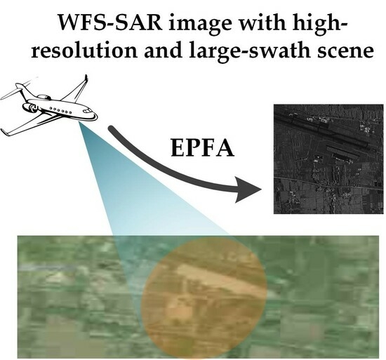
9]. A new imaging mode called widefield staring SAR (WFS-SAR) has been introduced to overcome the limitations of classic modes, which can offer sub-meter-level high-resolution images with large-swath scenes [10,11,12]. The implementation of WFS-SAR is mainly based on the expansion of spotlight mode, which can be arranged on linear or maneuvering trajectory motion platforms [13,14,15]. By reasonable beam shaping and control, a larger detection area can be obtained while ensuring high-resolution imaging. This advanced WFS-SAR mode offers superior performance and perfectly suits applications that demand high-resolution imaging over a wide area.
This paper considers a more complex and universal WFS-SAR imaging with maneuvering trajectory. As the spatial detection area expands and the time-frequency domain support area increases, frequency domain imaging algorithms based on transform domain approximation processing, such as range-doppler algorithm (RDA) [16,17], chirp-scaling algorithm (CSA) [18,19], and nonlinear CSA (NCSA) [20,21,22], will have significant residual phase error, which can adversely affect imaging performance. Although time domain imaging algorithms such as back-projection algorithm (BPA) and its modifications can be used for SAR imaging of any complex trajectory and work mode [23,24,25], they have strict requirements for navigation systems and digital signal processing systems, making them challenging to apply for real-time processing. The wavenumber domain polar format algorithm (PFA) is a typical spotlight SAR imaging method that eliminates spectrum aliasing through Deramp processing and achieves two-dimensional focusing through wavenumber spectrum resampling [26,27,28,29,30,31,32,33,34,35,36,37,38,39,40]. In addition, the implicit keystone transform in PFA can partly alleviate the range cell migration (RCM) caused by radar platform jitter and target motion, which can still effectively correct the RCM even with low inertial navigation accuracy or moving targets [28]. Therefore, it has inherent advantages in high-resolution imaging processing and can be further applied in WFS-SAR imaging.
However, PFA has a serious deficiency, as its derivation relies on a planar wavefront assumption that violates the actual situation [29,30]. Actually, the echo received by the radar antenna is a spherical wavefront in nature, and the neglected wavefront curvature phenomenon will affect the imaging results, leading to significant distortion and defocusing in the final image. The degree of distortion and defocusing increases with the distance away from the reference position during the PFA processing, exhibiting spatial variability, making it difficult to compensate through autofocusing and affine transformation [31]. Therefore, an essential step in PFA is to analyze and correct the wavefront curvature error (WCE).
A significant body of literature has been dedicated to exploring the wavefront curvature phenomenon. Doren [32,33] initially developed the wavefront curvature error and obtained the analytical expression of the WCE phase through an ideal model. Mao [28,34,35] gives a WCE phase suitable for level flight and diving motion and acquires good refocusing results through simulation experiments. The method presented in [36], which introduces a quadratic approximation of the differential slant range and derives the WCE phase through variable substitution, has a non-ignorable error in high-resolution and widefield SAR mode, despite being simple and easy to comprehend [37]. These methods are predicated on assuming the radar platform moves along an ideal linear trajectory. When the platform maneuvers along a complex trajectory, the inevitable acceleration will alter the echo azimuth modulation characteristics and cause image defocusing. Therefore, Deng [38,39] adopts an acceleration error compensation strategy combined with the WCE correction, which can achieve imaging processing of the maneuvering platform. However, the literature mentioned above only considers the impact of the quadratic component of WCE on image quality. As the resolution improves and the scene scale expands, the higher-order phase error will gradually increase and deteriorate the azimuth focusing performance. In addition, due to the coupling characteristics of the two-dimensional wavenumber domain variables, higher-order phase error will also affect the scattering point’s envelope. Therefore, in WFS-SAR imaging that considers both high-resolution and large-swath scenes, it is necessary to derive an accurate WCE phase in the two-dimensional wavenumber domain and conduct a specific analysis and evaluation on the neglected higher-order phase error.
In terms of WCE correction, the authors of [38] propose a local joint compensation method for spatially variant phase error and geometry distortion, which compensates for the WCE phase with each point while performing geometric correction. Although this method offers high accuracy in error compensation, it increases the algorithm’s computational complexity and poses challenges in integrating with motion compensation methods. Spatially variant inverse filtering [29,40] is a classic method for correcting WCE based on the gradual variability of the phase error. By dividing sub-images and compensating for the phase error in the transform domain, an acceptable focused image is obtained within the allowable error extent, resulting in a refocused SAR image with the cost of minimal increase in computational complexity.
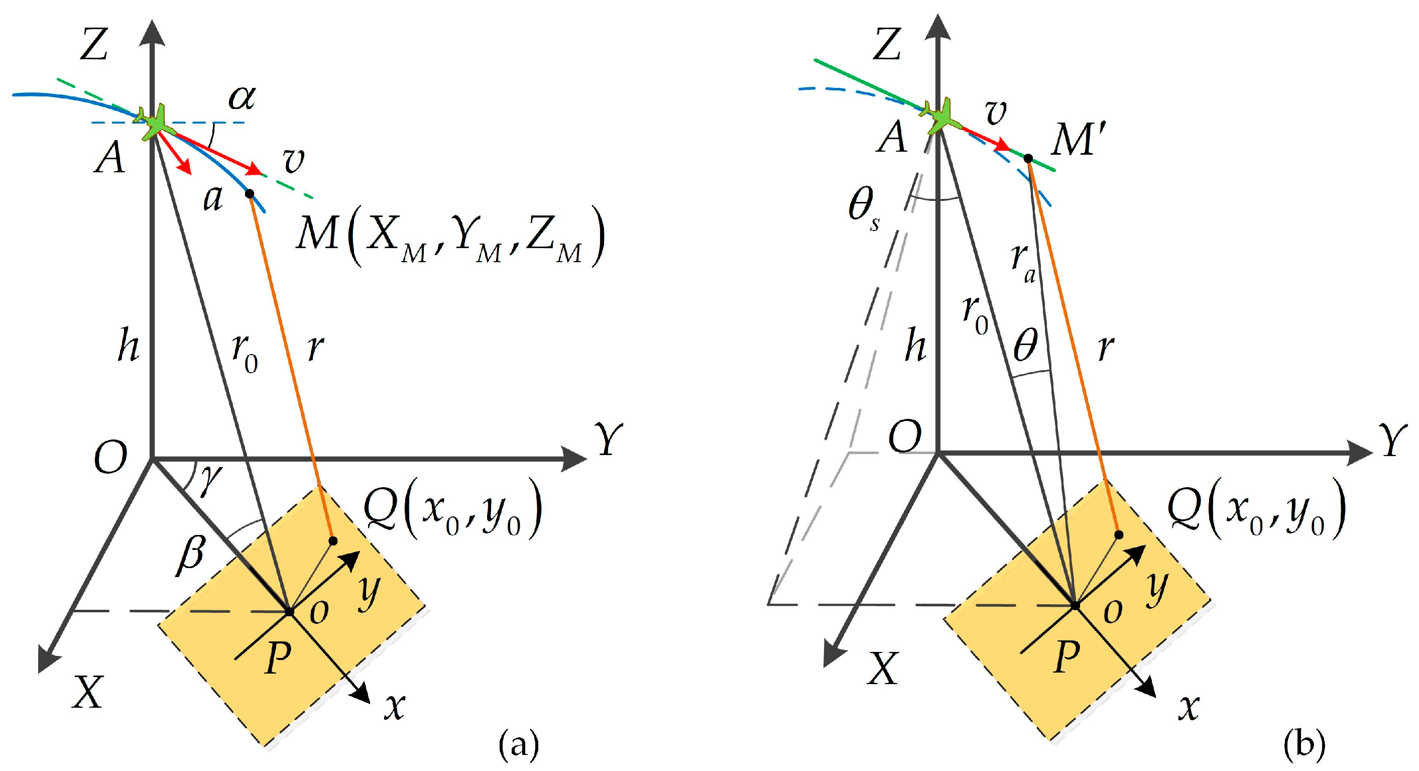
Aiming at the problem of WFS-SAR imaging with maneuvering trajectory, an extended polar format algorithm for joint envelope and phase error correction is proposed in this paper. Firstly, we establish a geometric model for maneuvering trajectory SAR imaging and construct an instantaneous slant range to obtain the baseband echo signal model. After acceleration compensation, the azimuth Deramp and two-dimensional resampling processing are performed to acquire a coarse-focused image on the slant range plane. Next, to eliminate the issue of image defocusing and distortion caused by the wavefront curvature phenomenon, we establish a mapping relationship between the geometry space and wavenumber space, and derive the WCE phase and residual acceleration error (RAE) phase by the McLaughlin series. On this basis, the joint envelope and phase correction function is proposed, and the phase error is accurately compensated through a sub-image processing strategy in the spatially variant inverse filtering. Finally, we obtain a well-focused and distortionless ground scene image through projection and geometric correction.
Compared with the existing algorithms, the main advantages of the proposed algorithm can be summarized as follows:
  • We associate the geometry space with wavenumber space based on the defined observation angle and derive an accurate analytical expression for the wavenumber domain signal.
  • We derive the WCE phase and RAE phase in polynomial form through the McLaughlin series, and evaluate the influence of the cubic phase error component on the scattering point envelope and azimuth focusing in the WFS-SAR imaging mounted on the maneuvering platform.
  • Relying on the spatially variant inverse filtering processing, we improve the traditional WCR phase compensation function and construct a new RCM recalibration function for joint envelope and phase error correction, which results in a well-focused maneuvering platform WFS-SAR image at the cost of a slight increase in computational complexity in the final.
This paper is organized as follows: In Section 2, a geometric model for WFS-SAR imaging with maneuvering trajectory is constructed, and the coarse-focused image is obtained through PFA imaging processing. Section 3 describes the proposed method for WCE correction in detail. The results of simulation experiments used to evaluate the proposed method are given in Section 4. Finally, the conclusions are drawn in Section 5.

2. PFA Imaging Processing

In this section, we establish a geometric model for WFS-SAR imaging with maneuvering trajectory and develop an echo signal model. Subsequently, PFA imaging processing is performed to generate a coarse-focused image on the slant range plane.

2.1. WFS-SAR Imaging Geometric Model

Taking the radar platform at the imaging center position as a reference, a spatial Cartesian coordinate system XOYZ is established by selecting the point below the aircraft as the coordinate origin O. The Y-axis represents the horizontal velocity direction, the X-axis represents the cross direction, and the Z-axis represents the sky direction, as shown in Figure 1a.
The SAR platform flies along a curved trajectory. Assuming that at the middle moment of the azimuth slow time, the platform is located at point A, with an altitude of h , and the flight velocity and acceleration vectors are v = 0 , v y , v z and a = a x , a y , a z , respectively. The centerline of the radar beam intersects with the ground plane at point P, which is selected as the scene reference position, and the slant range vector from the radar antenna pointing to point P is r 0 . For convenience, we define the elevation angle α as the angle between the horizontal plane and the flight velocity vector, the azimuth angle γ as the angle between the ground projection of the slang range vector and the positive direction of Y-axis, and the grazing angle β as the angle between the slant range vector and the ground plane. Using t m to denote the azimuth slow time, an arbitrary position M on the trajectory can be defined as:
X M = 1 2 a x t m 2 Y M = v t m cos α + 1 2 a y t m 2 Z M = v t m sin α + 1 2 a z t m 2 + r 0 sin β
where v = v represents the value of the velocity.
The target coordinate system xoy is established using the scene reference point P as the origin and the ground projection of the beam centerline as the positive direction of x-axis. For any point Q x 0 , y 0 in the target coordinate system, its actual position in the imaging coordinate system can be expressed as:
X Q = r 0 cos β sin γ + x 0 sin γ y 0 cos γ Y Q = r 0 cos β cos γ + x 0 cos γ + y 0 sin γ Z Q = 0
where r 0 = r 0 represents the value of the slant range. Therefore, the instantaneous slant range from the radar platform to the scattering point in the imaging scene can be expressed as:
r r e a l t m ; x 0 , y 0 = X M X Q 2 + Y M Y Q 2 + Z M Z Q 2
The azimuth dimensional high-resolution of synthetic aperture radar originated from the virtual antenna array formed by the continuous motion of the radar platform. However, high-order motion, such as acceleration, can disrupt the spacing among virtual array elements, resulting in a non-uniform distribution, further affecting the imaging performance of synthetic aperture radar. To solve this issue, we rewrite the slant range by separating the acceleration component and express the instantaneous slant range as a combination of uniform and higher-order motion terms.
r r e a l t m ; x 0 , y 0 = r t m ; x 0 , y 0 + r a c c t m ; x 0 , y 0
where r t m ; x 0 , y 0 represents the ideal uniform motion term and dictates azimuth resolution performance, r a c c t m ; x 0 , y 0 represents the disturbance term caused by acceleration, which can adversely affect the image quality, and hence must be compensated during imaging processing.
Supposing the radar emits the linear frequency modulation (LFM) signal, after matched filtering, we perform a range dimensional FFT on the received echo to obtain the signal in the range frequency domain.
S s f r , t m ; x 0 , y 0 = W r f r w a t m exp j 4 π f c + f r c r r e a l t m ; x 0 , y 0
among them, W r represents the range envelope in the time domain, w a represents the azimuth envelope in the frequency domain, f c represents the carrier frequency, f r represents the range frequency, and c represents the speed of light. We set k r = 4 π f r + f c / c to obtain the signal expression in the range wavenumber domain:
S s k r , t m ; x 0 , y 0 = W r k r w a t m exp j k r r r e a l t m ; x 0 , y 0 = W r k r w a t m exp j k r r t m ; x 0 , y 0 exp j k r r a c c t m ; x 0 , y 0
The acceleration component is involved in the second exponential phase of Equation (6), which is directly related to the scattering point position x 0 , y 0 within the imaging scene. Unfortunately, the signal support regions of scattering points overlap with each other in the range wavenumber domain, making it impossible to adjust the spatially variant phase uniformly. Therefore, we employ the origin of the target coordinate system as the reference to uniformly compensate for the consistent acceleration component in the wavenumber domain, as discussed in [14,38]. After unified compensation, the primary component of the high-order motion term has been corrected. Generally speaking, the RAE could be negligible when the imaging scene is small and the resolution is low. However, for WFS-SAR, which combines the characteristics of high-resolution and large scene, the RAE compensation is crucial. We will delve into this matter in greater detail in the succeeding section.
In practice, the acceleration information in SAR imaging is usually measured by accelerometers and transmitted to the signal processing system to support real-time SAR imaging processing. However, due to the influence of measurement noise, the output results of accelerometers often have certain deviations, which will introduce parameter errors and affect the focusing results. An effective processing method to solve this issue is integrating the acceleration to obtain velocity information containing errors, fitting it into an ideal uniformly accelerated motion model, and obtaining the reference acceleration and velocity parameters for SAR imaging processing. This will significantly reduce the impact of accelerometer measurement noise.

2.2. PFA Imaging Processing

After acceleration compensation, we can treat the radar’s movement as an ideal straight-line trajectory, as depicted in Figure 1b. Similar to traditional PFA, we construct an azimuth Deramp function in the wavenumber domain, which essentially compensates for the main component of the slant range with the scene center as the reference.
H D e r a m p k r , t m = exp j k r r a t m
where r a t m denotes the instantaneous center slant range, which represents the distance from an arbitrary point on the ideal trajectory to the origin of the imaging coordinate system, and yields:
r a t m = r 0 cos β sin γ 2 + r 0 cos β cos γ v t m cos α 2 + v t m sin α + r 0 sin β 2 = r 0 2 2 v t m r 0 sin θ s + v 2 t m 2
where θ s = arc sin cos α cos β cos γ sin α sin β represents the spatial squint angle, as shown in Figure 1b, which denotes the angle between the beam pointing and the zero Doppler plane.
Thus, the echo signal after azimuth Deramp processing can be represented as:
S s k r , t m ; x 0 , y 0 = W r k r w a t m exp j k r Δ r t m ; x 0 , y 0 = W r k r w a t m exp j Δ ϕ k r , t m ; x 0 , y 0
where Δ r t m ; x 0 , y 0 represents the differential slant range, which denotes the difference between the instantaneous slant range r t m ; x 0 , y 0 and the instantaneous center slant range r a t m , and correspondingly, Δ ϕ k r , t m ; x 0 , y 0 is called the differential phase.
The observation angle θ is defined as the angle between the radar beam pointing at an arbitrary moment and the azimuth middle moment, as depicted in Figure 1b. This angle signifies the variation of the spatial squint angle of the radar platform concerning the scene center during the synthetic aperture period. According to the geometric model, we can calculate the observation angle as the difference between the spatial squint angle at an arbitrary moment and the azimuth middle moment.
θ t m = a r c sin r 0 sin θ s v t m r a t m θ s = a r c sin v t m cos θ s r a t m
Meanwhile, the variation of the observation angle also reflects the process of synthetic aperture; therefore, the azimuth dimensional resolution can be expressed as:
ρ a = λ 2 Δ θ = λ 2 θ max θ min
where θ max and θ min represent the maximum and minimum values of the observation angle during the data acquisition period, respectively.
The essence of PFA is to retrieve phase history domain data sampled in polar coordinates format in the wavenumber space. However, the two-dimensional FFT struggles to effectively focus echo data in the polar coordinate format, making it necessary to convert sector sampled data into a Cartesian grid through resampling operations to achieve efficient focusing.
On the slant range plane, a set of Cartesian coordinate wavenumber variables k x , k y is defined along the beam centerline and vertical directions. The transformation relationship between polar coordinates and Cartesian coordinates can be expressed as:
k x = k r cos θ t m + π = k r cos θ t m k y = k r sin θ t m + π = k r sin θ t m
Coordinate system conversion can be achieved through two-dimensional resampling, and this process can be decomposed into two cascaded one-dimensional resampling in practice [31]. The range dimension resampling transforms polar format data into the trapezoidal format, which essentially changes the starting position and sampling interval of radial sampling through interpolation. The azimuth dimension resampling transforms trapezoidal format data into rectangular format, essentially changing the position of azimuth observation angle sampling through interpolation.
According to the above analysis, the differential phase after two-dimensional resampling can be rewritten as:
Δ ϕ k r , t m ; x 0 , y 0 = Δ ϕ k x , k y ; x 0 , y 0 = k x x 0 + k y y 0 + Δ ϕ k x , k y ; x 0 , y 0
The first two terms are the phase related to the target focusing position under the planar wavefront assumption, and the latter term is the phase error caused by the wavefront curvature phenomenon.
According to the planar wavefront assumption, ignoring the influence of the WCE phase, the resampled signal can be represented as:
S S k x , k y ; x 0 , y 0 W x k x w y k y exp j k x x 0 + k y y 0
Performing range IFFT and azimuth FFT on the signal yields the focusing result on the slant range plane:
s s x , y ; x 0 , y 0 = sin c Δ k x x x 0 sin c Δ k y y y 0
where Δ k x and Δ k y represent the wavenumber spectrum width in the range and azimuth dimensions, respectively. Up to now, the coarse-focused image has been obtained by PFA imaging processing.

3. Joint Envelope and Phase Error Correction

The planar wavefront assumption is adopted for PFA imaging processing in the previous section, while in reality, the echo received by the radar antenna is a spherical wavefront. Therefore, there exists a phase error Δ ϕ k x , k y ; x 0 , y 0 at all other points except for the scene reference position, which is a coupling function of the scattering point position x 0 , y 0 and the two-dimensional wavenumber variable k x , k y , and increases with the displacement of the scattering point and the expansion of the wavenumber spectrum width [37].
For WFS-SAR imaging with high-resolution and large scene, the quality of the focused image will be negatively impacted by the WCE. Specifically, the impact can manifest in two aspects. The first one is the displacement of the focusing position of the scattering point. The linear component concerned with the two-dimensional wavenumber variable k x , k y in the WCE phase Δ ϕ k x , k y ; x 0 , y 0 reflects displacement of the scattering point relative to its proper position, which varies with the proper position x 0 , y 0 , ultimately causing geometric distortion of the overall image. The second one is the deterioration of the focusing effect of the scattering point. The quadratic and higher-order components concerned with the two-dimensional wavenumber variable k x , k y in the WCE phase Δ ϕ k x , k y ; x 0 , y 0 worsen the azimuth focusing result. Similarly, due to the inherent spatial variability characteristics, the defocusing effect gradually becomes apparent as the scattering point moves away from the reference position.
Therefore, correcting the wavefront curvature phenomenon is the most crucial step in PFA-based WFS-SAR imaging processing. According to the analysis above, the WCE is related to radar spatial sampling and varies with the spatial position of scattering points. To accurately compensate for the WCE, it is essential to gather spatial location information from both the radar and scattering points. However, in the focusing domain, there is no wavenumber variable that can characterize the radar sampling information. Conversely, in the wavenumber domain, the wavenumber spectrum of scattering points overlaps with each other, making it impossible to handle the spatial variability of the scattering points’ position. This contradiction presents a significant challenge to the WCR correction.
In this section, the WCE phase will be divided into the defocused and distorted components, which are compensated by spatially variant inverse filtering and projection distortion correction, respectively.

3.1. Derivation of the Wavenumber Domain Signal

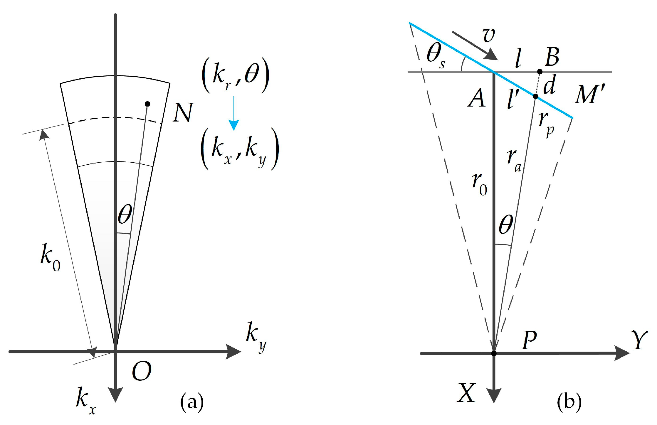
Before performing the WCE correction, it is necessary to derive the analytical expression for the wavenumber domain signal with the Cartesian coordinate format. Due to the two-dimensional resampling being implemented in coarse-focused imaging, it is difficult to obtain the WCE phase directly through variable substitution. However, by investigating the observation angle θ , we can express it as the arcsine value of the ratio of the lateral displacement within the instantaneous center slant range r a t m , as given in Equation (10). Simultaneously, it can also be expressed as the arctangent value of the ratio of the two-dimensional wavenumber variables, as shown in Figure 2a.
θ t m = arctan k y k x
Therefore, we can associate the variables in the geometry space and wavenumber space by the observing angle, and acquire the differential phase Δ ϕ k x , k y ; x 0 , y 0 through this relationship.
The diagram of the imaging slant range plane is shown in Figure 2b. We establish a right-hand coordinate system XPY with point P as the origin and the beam pointing AP as the X-axis at the azimuth middle moment. Assuming that at an arbitrary moment, the radar moves to point M , and the displacement of the radar platform concern to azimuth middle moment is l . Then, we extend the instantaneous center slant range r a in reverse and intersect with the Y-axis parallel line passing through point A at point B. We set AB as l , BP as r p , and B M as d , where l and r p represent the position displacement and instantaneous center slant range of the radar platform concern to azimuth middle moment in the side-looking mode, and d represents the difference between the instantaneous center slant range in the side-looking mode and squint mode.
θ = arctan l r 0
Combining Equations (16) and (17), the opposite l and the hypotenuse r p in triangle Δ A B P can be obtained, respectively, based on geometric relationships:
l = r 0 tan θ = r 0 k y k x
r p = r 0 2 + l 2 = r 0 1 + k y k x 2
Next, according to the sine theorem, there is a corresponding relationship between the three angles and three sides in triangle Δ A B M , and we can represent the other two edges through the known l :
d = l sin θ s cos θ θ s = r 0 Ω sin θ s 1 + k y k x 2
l = l cos θ cos θ θ s   =   r 0 Ω
where Ω is a factor, which yields:
Ω = k y / k x cos θ s k y / k x sin θ s
We use l to represent the position displacement of the radar platform and obtain a new instantaneous slant range r k x , k y ; x 0 , y 0 in the two-dimensional wavenumber.
r k x , k y ; x 0 , y 0 = r 0 cos β + x 0 + r 0 Ω cos α cos γ 2 + y 0 + r 0 Ω cos α sin γ 2 + r 0 sin β r 0 Ω sin α 2
Similarly, the new instantaneous center range slant r a k x , k y is obtained by subtracting d from r p .
r a k x , k y = r 0 1 + k y k x 2 1 + Ω sin θ s
Therefore, the accurate differential phase in the wavenumber domain can be rewritten as:
Δ ϕ k x , k y ; x 0 , y 0 = k x 2 + k y 2 r k x , k y ; x 0 , y 0 r a k x , k y
A common method to handle the complex formula is to approximate it as a power series [41,42]. Thus, we expand Δ ϕ k x , k y ; x 0 , y 0 concerning the two-dimensional wavenumber variable through the McLaughlin series to obtain the differential phase in the polynomial form.
Δ ϕ k x , k y ; x 0 , y 0 = k = 0 i + j = k a i j x 0 , y 0 k x i k y j
where k represents the McLaughlin expansion level, and k , i , and j are all natural numbers, a i j x 0 , y 0 represents the McLaughlin expansion coefficient, which yields:
a i j x 0 , y 0 = 1 i !   j ! i + j Δ ϕ k x , k y ; x 0 , y 0 k x i k y j
where i! represents the factorial from 1 to i. Among them, the linear term concerning the wavenumber variables represents the focusing position of the scattering point, while the quadratic and higher-order terms represent the defocusing phase caused by the wavefront curvature phenomenon.

3.2. Compensation for Wavefront Curvature Error

We know that the quadratic and higher-order components in the McLaughlin series expansion of the differential phase represent the defocused phase caused by the wavefront curvature phenomenon, which is the phase error that needs to be compensated in inverse filtering processing.
The existing literature [31,34] only considers the quadratic phase error (QPE) and neglects other high-order phase components, which have been proven to satisfy the requirements of conventional PFA imaging processing. However, we know that phase error is related to the position of scattering points and the width of the wavenumber spectrum. As the imaging scene expands and the resolution improves, the impact of higher-order phase error will gradually increase. Therefore, it is essential to explore the magnitude of cubic phase error (CER) and evaluate its effect on WFS-SAR imaging processing.
According to the McLaughlin series expansion formula shown in Equations (26) and (27), we can easily obtain the quadratic and cubic phase error coefficients of the differential phase Δ ϕ k x , k y ; x 0 , y 0 concerning the wavenumber variable k x , k y :
a 20 = 0 a 11 = 0 a 02 = 1 2 k 0 2 r 0 r c + 2 r 0 tan 2 θ s r 0 r 0 + 2 κ 3 sin θ s r c cos 2 θ s + κ 3 2 r 0 2 r c 3 cos 2 θ s a 30 = 0 a 21 = 0 a 12 = 1 2 k 0 2 2 r 0 cos 2 θ s 3 r 0 2 r c cos 2 θ s 4 r 0 x 0 κ 1 + r 0 x 0 cos β cos β r c 3 + r 0 4 + κ 1 sin θ s κ 2 2 κ 1 2 4 κ 2 r 0 x 0 cos β sin θ s r c 3 cos 2 θ s a 03 = 1 2 k 0 2 2 r 0 tan θ s 2 r 0 tan 3 θ s + κ 3 r 0 r c cos θ s + 2 r 0 sin θ s r 0 + κ 3 sin θ s r c cos 3 θ s r 0 2 κ 3 r 0 + 2 κ 3 sin θ s r c 3 cos 3 θ s + κ 3 3 r 0 3 r c 5 cos 3 θ s
where:
r c = r 0 2 + x 0 2 + y 0 2 + 2 x 0 r 0 cos β κ 1 = x 0 2 + y 0 2 κ 2 = r 0 cos α x 0 cos γ + y 0 sin γ κ 3 = r 0 sin θ s + cos α x 0 cos γ + y 0 sin γ
where r c represents the distance from the radar at the azimuth middle moment to an arbitrary point in the target coordinate system.
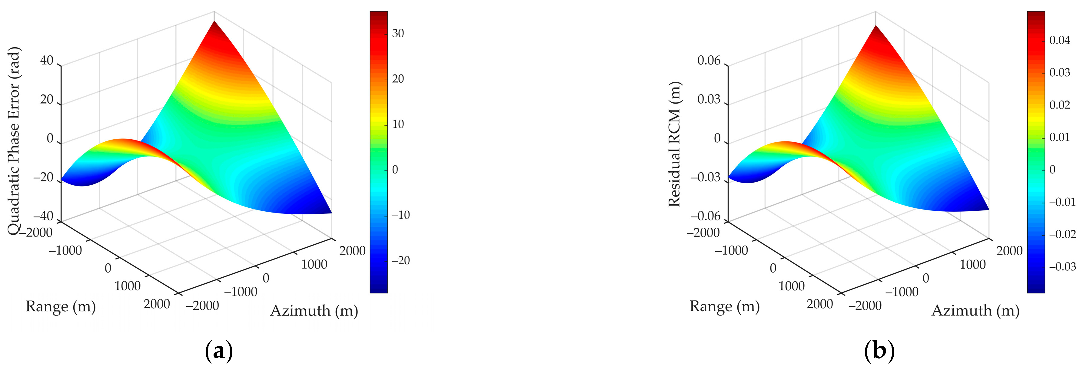
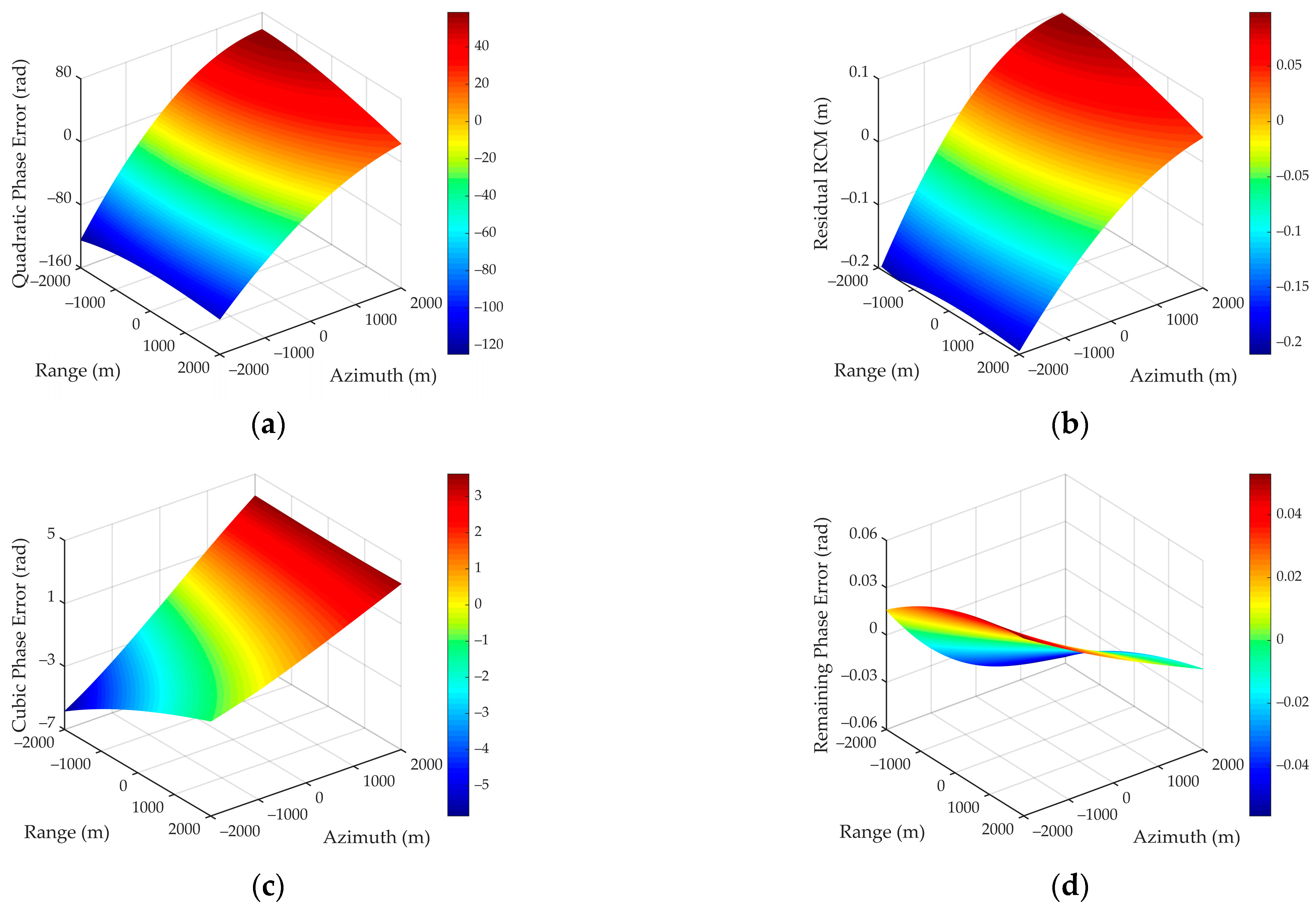
We can easily observe that only a 02 , a 12 , and a 03 exhibit non-zero values in the quadratic and cubic phase error coefficients. Among them, a 02 represents the quadratic term of the azimuth wavenumber, which is the main factor causing azimuth defocusing and the most crucial term in the WCE compensation. Additionally, a 12 represents the coupling term between the linear component of the range wavenumber and the quadratic component of the azimuth wavenumber, which reflects the variation of the range envelope with the azimuth position and is essentially the residual RCM caused by the WCE. Moreover, a 03 denotes the cubic term of the azimuth wavenumber, which is usually disregarded in conventional PFA imaging processing. However, its influence on azimuth focusing necessitates further evaluation for WFS-SAR imaging with high-resolution and large scenes.
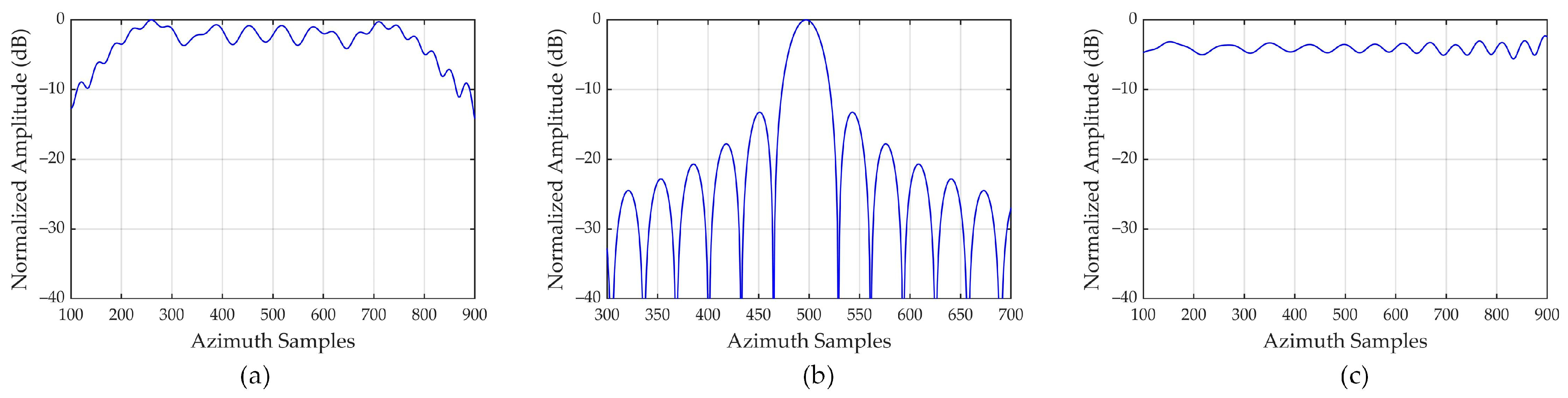
To intuitively present the extent of different error components, a simulation experiment is performed with typical parameters shown in Table 1. Simulation results are given in Figure 3. It is easy to notice that the quadratic phase error caused by a 02 exceeds 30 radians in Figure 3a, which is undoubtedly the primary issue to be addressed. The residual RCM caused by a 12 is less than 0.05 m, shown in Figure 3b, which is negligible when considering a sampling interval of 0.3 m, as half or a quarter of the sampling interval is usually used as the error threshold. Furthermore, the cubic phase error caused by a 03 exceeds π / 4 in Figure 3c, thus making it necessary to compensate for this term, as π / 4 or even π / 8 is generally considered an acceptable error margin. Figure 3d shows the remaining phase error beyond the quadratic and cubic terms with the value less than 0.005 rad, indicating that the remaining phase error is small enough to be negligible.
Therefore, we must compensate for the quadratic and cubic phase errors caused by the WCR to ensure azimuth-focusing performance, while the residual RCM can be temporarily ignored. Based on the analysis results, a WCE compensation function is constructed.
H W C E c o m k y ; x 0 , y 0 = exp j a 02 x 0 , y 0 k y 2 + a 03 x 0 , y 0 k y 3
This equation can achieve an accurate compensation for the WCE of the scattering point at x 0 , y 0 in the imaging scene.
After obtaining the error compensation function, how to perform the WCE compensation on the coarse-focused image is also an important issue. Considering the gradual variation of error with the position of scattering points, spatially variant inverse filtering is a typical and efficient wavefront curvature correction strategy. We first divide the coarse-focused image into sub-images based on the criterion that ensures the phase error change within the sub-image is less than π / 4 . Subsequently, the sub-image is transformed into the azimuth wavenumber domain, and a WCE compensation function is constructed with its center as a reference. After completing the error compensation, it returns to the focusing domain to obtain an accurately focused sub-image. Finally, the refocused image is acquired through sub-image stitching. It should be noted that the keynote of this paper is to discuss the impact of higher-order components in the WCE on imaging performance when using PFA for WFS-SAR imaging, while we will not elaborate on sub-image segmentation and stitching methods in detail.

3.3. Compensation for Residual Acceleration Error

In the previous section, we use the origin of the target coordinate system to uniformly compensate for high-order motion, and the residual error can be expressed as:
Δ r a c c t m ; x 0 , y 0 = r a c c t m ; x 0 , y 0 r a c c t m ; 0 , 0
It is easy to know that Δ r a c c t m ; x 0 , y 0 is also an error related to the position of scattering points. According to the characteristics of the echo signal, the RAE phase in the range wavenumber domain can be expressed as:
Δ ϕ a c c k r , t m ; x 0 , y 0 = k r Δ r a c c t m ; x 0 , y 0
As the resolution improves and the imaging area expands, the RAE phase Δ ϕ a c c k r , t m ; x 0 , y 0 gradually increases and cannot be ignored. Therefore, it is imperative to analyze and compensate for the phase error in the WFS-SAR imaging mode.
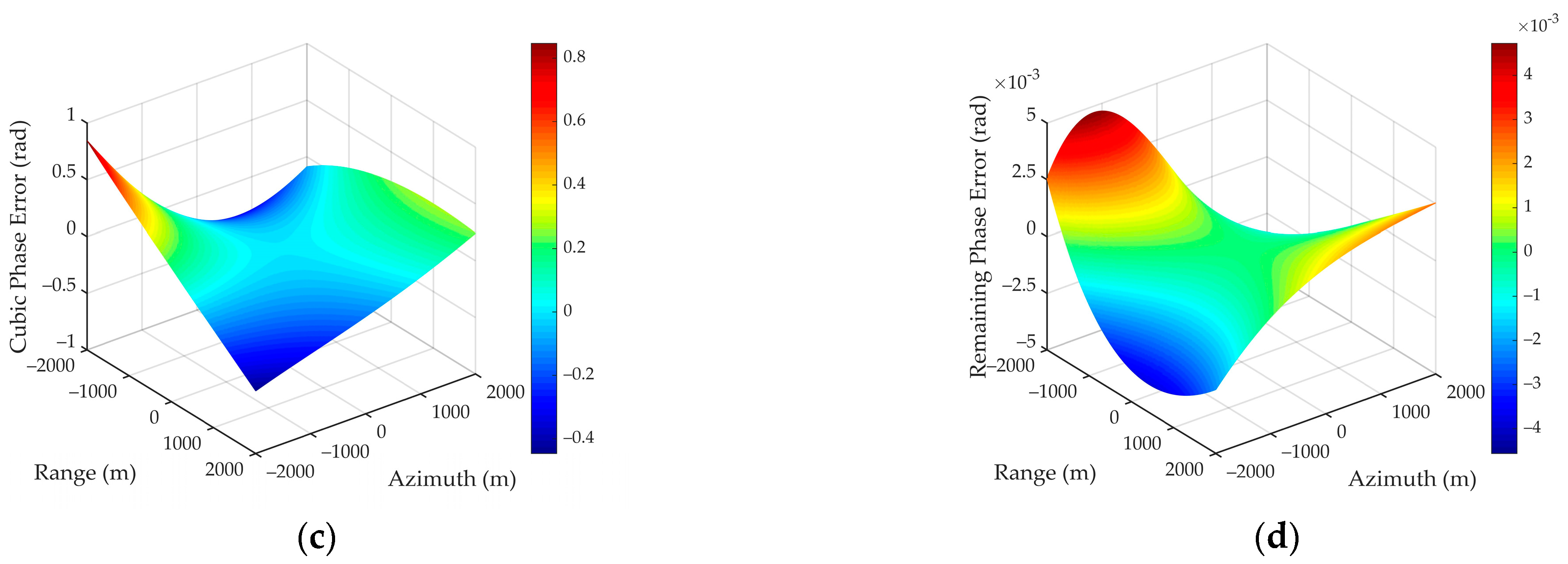
Since the RAE phase varies with the scattering point’s position, which is similar to the WCE phase, we consider performing the error analysis using the same method. Based on the correspondence between the geometry and wavenumber space established earlier, a similar method is used to map the RAE phase to the wavenumber domain, and it is expanded by the McLaughlin series to obtain the residual acceleration error in polynomial form.
Δ ϕ a c c k x , k y ; x 0 , y 0 = k = 0 i + j = k b i j x 0 , y 0 k x i k y j
where:
b 10 = 0 b 01 = 0 b 20 = 0 b 11 = 0 b 02 = a x x 0 + a y y 0 r 0 2 + a x cos β a z sin β r 0 r c r 0 2 k 0 r c cos 2 θ s b 30 = 0 b 21 = 0 b 12 = a x x 0 + a y y 0 r 0 2 + a x cos β a z sin β r 0 r c r 0 2 k 0 2 r c cos 2 θ s b 03 = r 0 2 2 r c 2 sin θ s + r 0 2 sin α sin β a x x 0 + a y y 0 + r 0 2 r 0 3 + r c 3 κ 4 + κ 5 + a z sin α + r 0 3 κ 1 a z sin α 2 sin β sin θ s + r 0 3 κ 2 a z sin β + 2 r 0 3 a x κ 1 sin θ s + 2 r 0 x 0 κ 5 cos β r 0 3 a x y 0 a y x 0 x 0 sin γ y 0 cos γ cos α + 2 r 0 4 x 0 a y cos α sin γ + a z sin α cos β r 0 4 y 0 a x sin γ + a y cos γ cos α cos β k 0 2 r c 3 cos 3 θ s
where:
κ 4 = a x cos γ + a y sin γ cos α κ 5 = a x cos β a z sin β sin θ s
Based on the results shown above, it can be concluded that the RAE phase and the WCE phase have similar spatially variant characteristics since only the values of b 02 , b 12 , and b 03 are not equal to zero in all expansion terms. Among them, b 02 represents the quadratic term of the azimuth wavenumber, which is the most crucial term in the RAE phase compensation. Here, b 12 represents the coupling term between the linear component of the range wavenumber and the quadratic component of the azimuth wavenumber, which reflects the residual RCM brought by acceleration, and its impact needs further evaluation. Additionally, b 03 represents the cubic term of the azimuth wavenumber, which theoretically has a smaller value. However, for the WFS-SAR mode with more stringent imaging conditions, its impact on azimuth focusing performance also needs to be further evaluated.
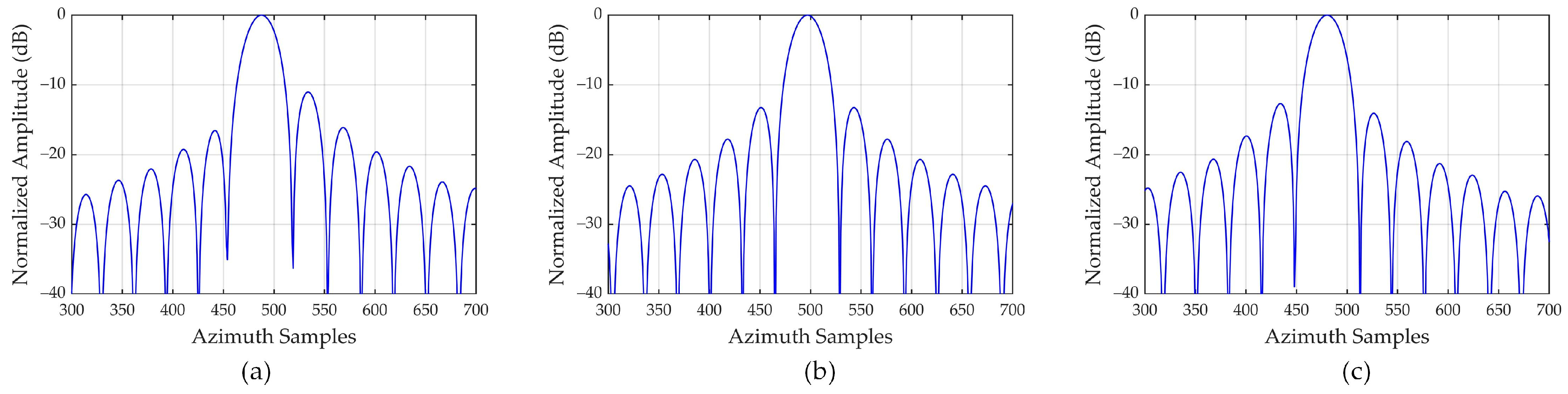
Next, we will simulate the phase error caused by the residual acceleration. Parameters are shown in Table 1, and simulation results are given in Figure 4. It is easy to find that in Figure 4a, the quadratic phase error caused by b 02 exceeds 160 rad, which is the main component of the RAE, and its value even exceeds the WCE. The residual RCM caused by b 12 in Figure 4b exceeds 0.2 m, which has outnumbered the error threshold of half of the sampling interval. Thus, further correction of residual RCM is also required. In addition, the phase error caused by b 03 exceeds 5 rad, as shown in Figure 4c, which is an indispensable item in error compensation. Figure 4d shows the remaining higher-order phase error beyond the quadratic and cubic components, which can be ignored with a maximum value of approximately 0.05 rad.
According to the simulation results, we construct a residual acceleration error compensation function and a range cell migration recalibration function:
H A C C c o m k y ; x 0 , y 0 = exp j b 02 x 0 , y 0 k y 2 + b 03 x 0 , y 0 k y 3
H A C C R C M C k x , k y ; x 0 , y 0 = exp j b 12 x 0 , y 0 k x k y 2
It is easy to find that the RAE phase shown in Equation (36) can be universally processed in the spatially variant inverse filtering together with the WCE phase. The RCM shown in Equation (37) must be corrected by transforming the sub-image into the two-dimensional wavenumber domain, which is also an essential processing module in WFS-SAR imaging.
Furthermore, considering that residual acceleration compensation needs to undergo the two-dimensional wavenumber domain, we can also correct the RCM caused by the WCE while performing RCM recalibration to improve our method’s robustness and universality. The recalibration function can be expressed as:
H W C E R C M C k x , k y ; x 0 , y 0 = exp j a 12 x 0 , y 0 k x k y 2

3.4. Projection and Geometric Correction

In the previous part, the WCE and RAE compensation functions are derived, and the strategy of inverse filtering based on sub-image processing is explained. Next, we will analyze the problem of the scattering point position distortion caused by wavefront curvature phenomena in detail.
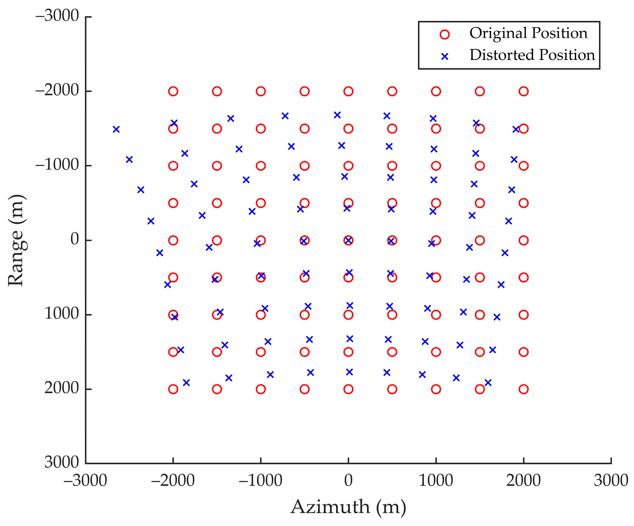
As mentioned earlier, in the McLaughlin series expansion of the differential phase, the linear term of the wavenumber variable represents the scattering point focusing position. The exact analytical expression for the focusing position can be obtained through Equation (27).
x p = a 10 = r c r 0
y p = a 01 = r 0 cos α x 0 cos γ + y 0 sin γ + r 0 sin θ s r c cos θ s r 0 tan θ s
The equations shown above indicate that the scattering point located at x 0 , y 0 in the target coordinate system is focused at x p , y p 
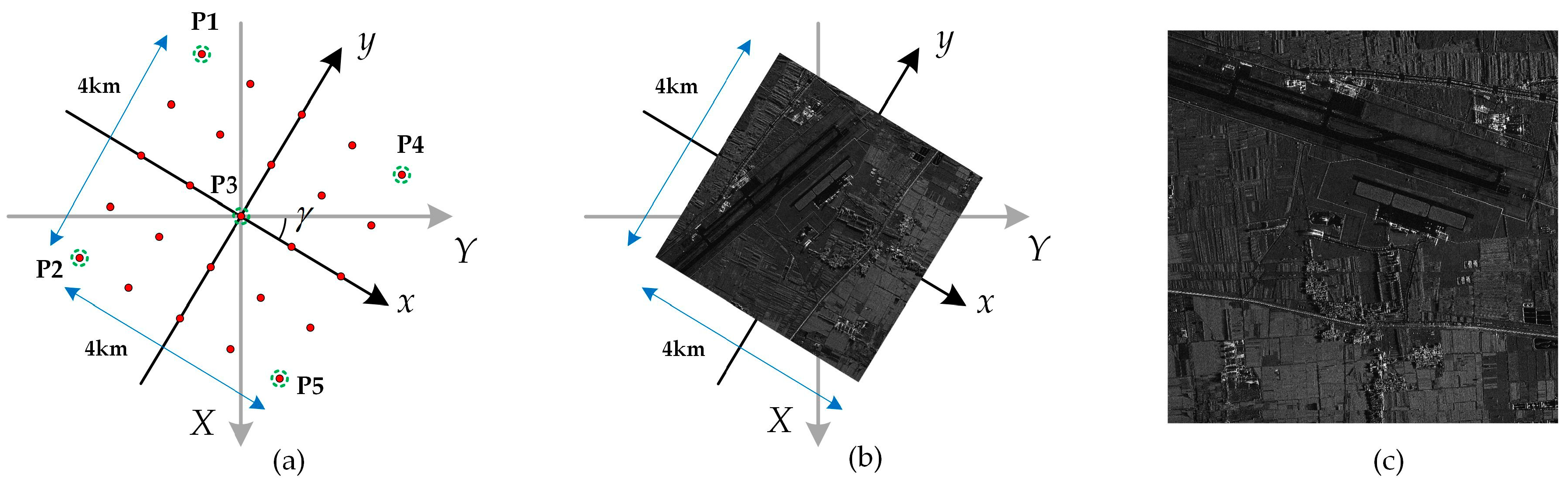
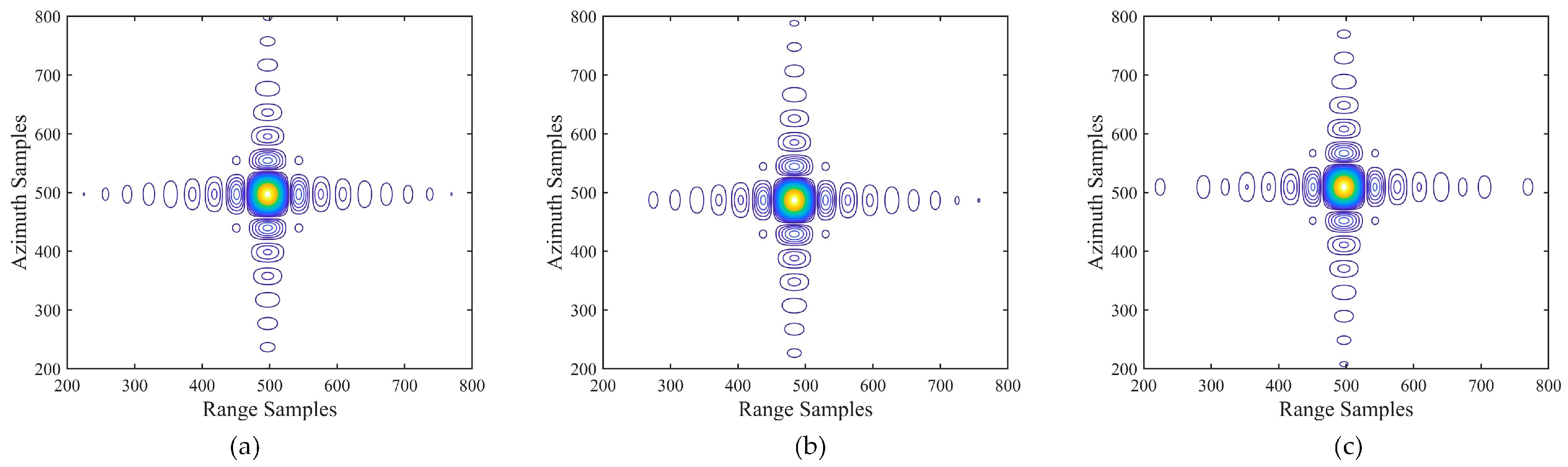
after PFA imaging processing, which is the position distortion caused by the WCE. To present the position distortion phenomenon more intuitively, we conducted a simple simulation using a point array, and parameters are also given in Table 1.
From the simulation result depicted in Figure 5, it can be observed that the extent of image distortion in the slant range plane increases as the displacement of the scattering point, ultimately changing the geometric shape and relative position relationship of the imaging area, resulting in the entire scene appearing as an irregular sector.
Since the actual terrain features cannot be accurately presented in the focused image on the slant range plane, it is necessary to perform the projection and distortion correction. We adopt the theory of reverse projection and locate the scattering point position through the distortion relationship shown in Equations (39) and (40), thereby enabling the retrieval of amplitude and phase information [29,39]. Further details on this process are provided in the following.
Step 1: Form a pixel grid in the target coordinate system based on a fixed resolution interval and number of image points.
Step 2: For an arbitrary point P x 0 , y 0 within the pixel grid, calculate its distorted position x p , y p on the focused image using Equations (39) and (40).
Step 3: Take a data block of size M × M with x p , y p as the reference and obtain the amplitude and phase information through interpolation.
Step 4: Traverse all grid points to obtain a well-focused ground plane image without distortion.
We can adopt different interpolation kernels according to accuracy requirements in practice, and select the size M of the data block based on the interpolation kernel.
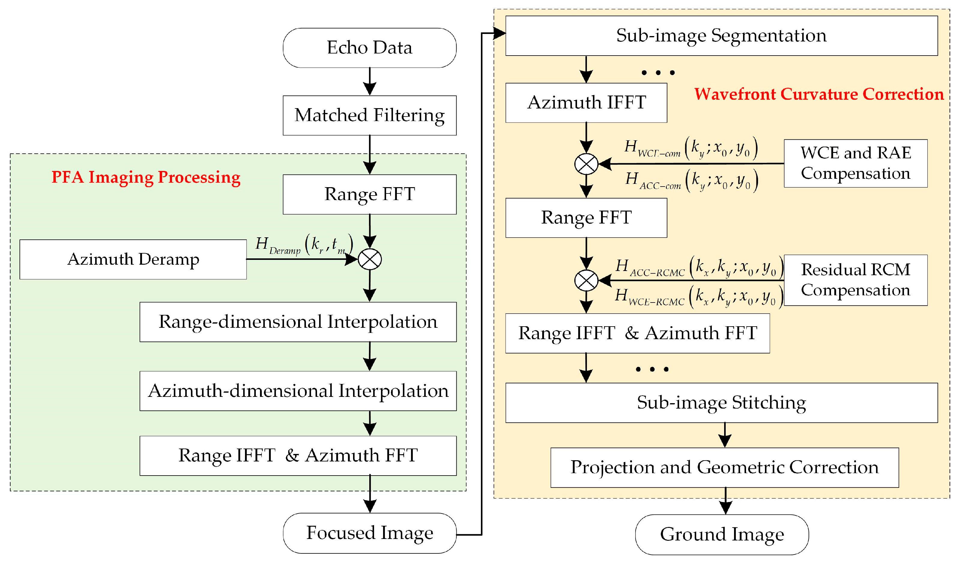
The processing flow of this algorithm is shown in Figure 6.

3.5. Computational Complexity

For engineering applications, we need to analyze the computational complexity of the proposed algorithm. It is well known that the calculation amount of N-point FFT/IFFT is 5 N log 2 N , the calculation amount of N-point complex phase multiplication is 6 N , and the calculation amount of N-point M-kernel sinc interpolation is 2 2 M 1 N .
In the coarse-focused processing of PFA, the algorithm involves two instances of FFT/IFFT in the range dimension, one instance of FFT/IFFT in the azimuth dimension, one instance of phase multiplication, and two instances of interpolation. Supposing N r and N a denote the range and azimuth dimension sampling number, respectively, the computational complexity of coarse-focused processing can be expressed as:
C C o a r s e = 10 N r N a log 2 N r + 5 N r N a log 2 N a + 6 N r N a + 4 2 M 1 N r N a
It is consistent with the computational burden of traditional interpolation-based PFA.
In the proposed algorithm, we compensate for the WCE and RAE through the spatially variable inverse filtering. Assuming that the range and azimuth dimension points of the sub-image are both N s u b , and considering half of the azimuth dimension overlap width, the computational complexity of the joint envelope and phase error correction can be expressed as:
C J E P E = 40 N r N a log 2 N s u b + 24 N r N a
Therefore, the computational complexity of the proposed algorithm can be calculated by C P F A = C C o a r s e + C J E P E .
Although the proposed algorithm partly increases the computational burden compared to others, it can precisely focus the entire scene in WFS-SAR imaging with high-resolution and large scene. Therefore, this phenomenon is acceptable in practice.

4. Simulation Experiments

Simulation experiments are conducted in this section to verify the effectiveness of the extended polar format algorithm proposed in this paper. Typical simulation parameters are given in Table 1.
Simulation experiments are divided into three parts. The first and second parts concentrate on the PFA imaging processing of scattering point targets without and with acceleration, respectively, and demonstrate the accuracy of the wavefront curvature correction method and residual acceleration compensation method through a detailed analysis of the focusing result. Subsequently, the distributed target is further simulated in the last part to verify the focusing performance of the proposed method.

4.1. Simulation of Scattering Point Target without Acceleration

The effectiveness of the proposed WCE compensation method with linear trajectory is presented in this part. Assume that the swath of the WFS-SAR imaging area is 4 km in the range and azimuth direction, in which a 5 × 5 point array is uniformly arranged to imitate scattering points at different positions. As shown in Figure 7a, we mark five points in the imaging area for subsequent analysis, where P1, P2, P4, and P5 are located at the edge positions with significant phase errors, and P3 located at the scene center is selected as a reference point. In addition, we introduce a reference method [34] as a comparison to verify the effectiveness of the method proposed in this paper.
Figure 8 shows the azimuth profiles of scattering points after PFA imaging processing. Due to the significant WCE phase that cannot be ignored, points P2 and P5 located at the edge position experience severe defocusing, which will seriously lose image information and cannot be accepted.
In comparison, the azimuth profiles of the WCE correction result mentioned in [34] are given in Figure 9, which is equivalent to only considering the quadratic phase error component in Equation (28). From Figure 9a,c, it can be seen that the focusing performance of the scattering points has been greatly improved. However, due to the undeniable cubic phase error, the side-lobe of points P2 and P5 exhibit asymmetry. Additionally, the azimuth profiles shown in Figure 9 show the result of accurate error compensation. In practice, an uncertain position mismatch error is introduced based on spatially variant inverse filtering, which further deteriorates the azimuth focusing result.
Figure 10 shows the azimuth profiles from the proposed WCE correction method proposed in this paper. Based on the reference method, we consider the influence of cubic phase error and eliminate the phenomenon of side-lobe asymmetry at edge points. By precisely compensating for the third-order phase component, the remaining phase error is small enough to be negligible in the azimuth focus. Therefore, the azimuth profiles of edge points P2 and P5 are nearly identical to the central reference point P3. The contour plots through the proposed method are displayed in Figure 11, proving that the main lobe and side lobes are separated clearly, presenting an ideal “cross”.
In addition, to further evaluate the imaging performance of the proposed algorithm, we make statistics on two-dimensional resolutions, as well as the peak side-lobe ratio (PSLR) and integrated side-lobe ratio (ISLR) of the azimuth profile. Results are readily available in Table 2. By comparison, it is evident that our algorithm boasts the lowest PSLR and ISLR values, which closely approach the ideal values of −13.26 dB and −9.80 dB.

4.2. Simulation of Scattering Point Target with Acceleration

Based on the simulation model established in the previous part, we take scattering points P2, P3, and P4 to verify the effectiveness of the RAE compensation method under the condition of maneuvering trajectory motion. A set of typical acceleration parameters are presented in Table 1.
Figure 12 shows the azimuth profiles of three scattering points following the implementation of the WCE correction mentioned in this paper. Apparently, the phase error caused by the residual acceleration results in severe azimuth defocusing. A comparative result reveals that the impact of RAE is even greater than that of WCE, which aligns with the analysis results in the preceding section.
The azimuth profiles of residual acceleration compensation result discussed in [38] are depicted in Figure 13. Similarly, the literature only considers the quadratic phase error and ignores other higher-order errors, resulting in significant asymmetry in the side lobes of the scattering points located at edge positions. Figure 13a shows that the first side lobe on the left side of point P1 is integrated into the main lobe, causing the main lobe to widen. In addition, the elevation of the remaining side lobes causes continuous ghosting, seriously deteriorating image performance.
Figure 14 displays the azimuth profiles of the RAE compensation result proposed in this paper. Due to the additional consideration of the cubic phase error, the side lobes of all scattering points exhibit left-right symmetry. They are consistent with the central reference point in the azimuth profile, presenting an anticipated ideal focusing outcome. The contour plots corresponding to Figure 14 are given in Figure 15. Unfortunately, the two-dimensional envelopes of the scattering points in Figure 15a are coupled, and the contour lines exhibit distorted characteristics. This phenomenon can be attributed to the residual RCM caused by the RAE; therefore, it is imperative to recalibrate the residual RCM in WFS-SAR mode.
In spatially variant inverse filtering processing, the sub-image is transformed into the two-dimensional wavenumber domain for residual RCM correction, resulting in the contour plots with two orthogonal envelopes, as shown in Figure 16. The main lobe and side lobes are separated clearly, presenting an ideal “cross”.
Similarly, we perform a statistical analysis on the two-dimensional resolution, and the PSLR and ISLR of the azimuth profile. The results are compiled in Table 3. By comparison, it can be found that after compensating for the cubic phase error derived by us, the azimuth resolution of the edge point returns to normal. In addition, the PSLR and ISLR of the proposed algorithm are the lowest, close to the desired −13.26 dB and −9.80 dB. These results prove the effectiveness of the compensation method for spatial acceleration error proposed in this algorithm.

4.3. Simulation of Distributed Target

To further illustrate the imaging performance of the proposed method in complex imaging scenes, an actual SAR image in the same band is selected as a benchmark image for distributed target simulation. The benchmark image layout is similar to the distribution of the point array, as illustrated in Figure 7b,c. During the simulation experiment, each pixel in the benchmark image is treated as an independent scattering point, and the entire image size is 4 km. Simulation parameters are based on the values in Table 1.
Simulation results of the distributed target are shown in Figure 17, where Figure 17a,b represent the image before and after phase compensation, respectively. In Figure 17a, it can be seen that as the scattering point deviates, the image gradually becomes defocused until wholly blurred, and the effective scene only covers a part of the area near the center reference position. By comparison, due to the compensation for the WCE and RAE, the image details of the entire scene can be clearly presented in Figure 17b, indicating that phase error compensation is a crucial step in PFA imaging.
Furthermore, an enlarged view of the edge area marked by the yellow rectangle in the focused image is provided in Figure 18, where Figure 18a,b are derived from the reference method [38] and the proposed method, respectively. Due to the consideration of cubic phase effects on the basis of traditional quadratic phase error, the focusing results of isolated scattering points in Figure 18b are better than those in Figure 18a.
In addition, we chose two isolated scattering points in the enlarged image for a more intuitive comparison, where a green circle marks P6 and P7 with a yellow circle, and the comparison results of their azimuth profiles are shown in Figure 19. The blue dotted line is the azimuth profile of the reference method. Since the impact of the cubic phase is neglected in [38], the side lobe level of scattering points is exceptionally high, and the main lobe even splits into multiple parts, leading to the generation of false targets and seriously deteriorates image quality. On the contrary, since the influence of the cubic phase error has been considered in our method, the azimuth profile of the scattering points has narrower main lobes and lower side lobes, indicating that the algorithm proposed in this paper has a better-focusing performance, as shown by the white line in Figure 19.
Finally, comparing Figure 17b with Figure 5, they have the same distortion characteristics, which further verifies the correctness of the distortion relationship in Equations (39) and (40). Through the projection and distortion correction processing described in this paper, the ground plane image of the distributed target is shown in Figure 20. The most apparent curved airport runway in Figure 17b has been corrected to a straight line, which is similar to the benchmark image shown in Figure 7c, further demonstrating the effectiveness of the projection and distortion correction method.

5. Conclusions

In this paper, an extended polar format algorithm for joint envelope and phase error correction in WFS-SAR imaging with maneuvering trajectory is proposed. We first establish a geometric model for maneuvering platform SAR imaging and obtain a coarse-focused result in the slant range plane through classical PFA imaging processing. Next, a mapping relationship between the geometry space and wavenumber space is constructed based on the observation angle, and the signal is converted into the wavenumber domain. Subsequently, we analyze the WCE phase and the RAE phase in detail, propose a refocusing function containing the cubic phase, and construct a novel RCM recalibration function. Finally, the two-dimensional precisely focused SAR image is acquired based on the spatially variant inverse filtering. The wavefront curvature correction method proposed in this paper is suitable for maneuvering platform WFS-SAR imaging with high-resolution and large scenes, which can be further applied to the fields of detection and reconnaissance.

Author Contributions

Conceptualization, Y.L. (Yujie Liang) and Y.L. (Yi Liang); methodology, Y.L. (Yujie Liang); software, Y.L. (Yujie Liang) and X.W.; validation, Y.L. (Yi Liang) and J.L.; formal analysis, J.L.; resources, Y.L. (Yi Liang) and M.X.; writing—original draft preparation, Y.L. (Yujie Liang); writing—review and editing, X.W.; visualization, Y.L. (Yujie Liang) and X.W.; supervision, Y.L. (Yi Liang) and M.X.; funding acquisition, Y.L. (Yi Liang). All authors have read and agreed to the published version of the manuscript.

Funding

This work was supported by the National Natural Science Foundation of China under Grant 61971326.

Data Availability Statement

No new data were created or analyzed in this study. Data sharing is not applicable to this article.

Acknowledgments

We would like to thank the editors and anonymous reviewers for their valuable comments to improve the paper quality.

Conflicts of Interest

The authors declare no conflicts of interest.

References

  1. Cumming, I.G.; Wong, F.H. Digital Processing of Synthetic Aperture Radar Data: Algorithms and Implementation; Artech House: Norwood, MA, USA, 2005; pp. 3–17. [Google Scholar]
  2. Moreira, A.; Prats-Iraola, P.; Younis, M.; Krieger, G.; Hajnsek, I.; Papathanassiou, K.P. A tutorial on synthetic aperture radar. IEEE Geosci. Remote Sens. Mag. 2013, 1, 6–43. [Google Scholar] [CrossRef]
  3. Mccorkle, J.W. Focusing of synthetic aperture ultra wideband data. In Proceedings of the IEEE International Conference on Systems Engineering, Dayton, OH, USA, 1–3 August 1991. [Google Scholar]
  4. Lawton, W. A New Polar Fourier Transform for Computer-Aided Tomography and Spotlight Synthetic Aperture Radar. IEEE Trans. Acoust. Speech Signal Process. 1988, 36, 931–933. [Google Scholar] [CrossRef]
  5. Nies, H.; Loffeld, O.; Natroshvili, K. Analysis and Focusing of Bistatic Airborne SAR Data. IEEE Trans. Geosci. Remote Sens. 2007, 45, 3342–3349. [Google Scholar]
  6. Liu, W.K.; Sun, G.C.; Xia, X.G.; Chen, J.L.; Guo, L.; Xing, M.D. A Modified CSA Based on Joint Time-Doppler Resampling for MEO SAR Stripmap Mode. IEEE Trans. Geosci. Remote Sens. 2018, 56, 3573–3586. [Google Scholar] [CrossRef]
  7. Mittermayer, J.; Moreira, A.; Loffeld, O. Spotlight SAR Data Processing Using the Frequency Scaling Algorithm. IEEE Trans. Geosci. Remote Sens. 1999, 37, 2198–2214. [Google Scholar] [CrossRef]
  8. Zhu, D.Y.; Ye, S.H.; Zhu, Z.D. Polar Format Algorithm using Chirp Scaling for Spotlight SAR Image Formation IEEE Trans. Aerosp. Electron. Syst. 2008, 44, 1433–1448. [Google Scholar] [CrossRef]
  9. Liao, Y.; Xing, M.D.; Bao, Z. Imaging algorithm for circular trace scanning synthetic aperture radar using modified hyperbolic range equation. Electron. Lett. 2013, 49, 1296–1298. [Google Scholar] [CrossRef]
  10. Nie, X.; Shen, S.J.; Yu, H.; Liu, Y.; Zhuang, L.; Lei, W. A wide-field SAR polar format algorithm based on quadtree sub-image segmentation. In Proceedings of the IEEE International Geoscience and Remote Sensing Symposium, Valencia, Spain, 22–27 July 2018. [Google Scholar]
  11. Fan, B.; Qin, Y.L.; You, P.; Wang, H.Q. An Improved PFA with Aperture Accommodation for Widefield Spotlight SAR Imaging. IEEE Geosci. Remote Sens. Lett. 2015, 12, 3–7. [Google Scholar] [CrossRef]
  12. Meng, Z.C.; Zhang, L.; Chen, L.L. Widefield Parametric Polar Format Algorithm for Spotlight SAR Imaging. IEEE J. Sel. Top. Appl. Earth Obs. Remote Sens. 2023, 16, 7293–7302. [Google Scholar] [CrossRef]
  13. Liang, Y.; Dang, Y.F.; Li, G.F.; Wu, J.X.; Xing, M.D. A Two-Step Processing Method for Diving-Mode Squint SAR Imaging with Subaperture Data. IEEE Trans. Geosci. Remote Sens. 2020, 58, 811–825. [Google Scholar] [CrossRef]
  14. Li, Z.Y.; Xing, M.D.; Liang, Y.; Gao, Y.X.; Chen, J.L.; Huai, Y.Y.; Sun, G.C.; Bao, Z. A Frequency-Domain Imaging Algorithm for Highly Squinted SAR Mounted on Maneuvering Platforms with Nonlinear Trajectory. IEEE Trans. Geosci. Remote Sens. 2016, 54, 4023–4038. [Google Scholar] [CrossRef]
  15. Zhang, G.; Liang, Y.; Suo, Z.Y.; Xing, M.D. Modified ERMA with Generalized Resampling for Maneuvering Highly Squinted TOPS SAR. IEEE Geosci. Remote Sens. Lett. 2022, 19, 1–5. [Google Scholar] [CrossRef]
  16. Neo, Y.N.; Wong, F.H.; Cumming, I.G. Processing of Azimuth-Invariant Bistatic SAR Data Using the Range Doppler Algorithm. IEEE Trans. Geosci. Remote Sens. 2008, 46, 14–23. [Google Scholar] [CrossRef]
  17. Guo, Y.N.; Wang, P.B.; Men, Z.R.; Chen, J.; Zhou, X.K.; He, T.; Cui, L. A Modified Range Doppler Algorithm for High-Squint SAR Data Imaging. Remote Sens. 2023, 15, 4200. [Google Scholar] [CrossRef]
  18. Chen, S.; Zhang, S.N.; Zhao, H.C.; Chen, Y. A New Chirp Scaling Algorithm for Highly Squinted Missile-Borne SAR Based on FrFT. IEEE J. Sel. Top. Appl. Earth Obs. Remote Sens. 2015, 8, 3977–3987. [Google Scholar] [CrossRef]
  19. Davidson, G.W.; Cumming, I.G.; ITO, M.R. A Chirp Scaling Approach for Processing Squint Mode SAR Data. IEEE Trans. Aerosp. Electron. Syst. 1996, 32, 121–133. [Google Scholar] [CrossRef]
  20. Li, Z.Y.; Liang, Y.; Xing, M.D.; Huai, Y.Y.; Zeng, L.T.; Bao, Z. Focusing of Highly Squinted SAR Data with Frequency Nonlinear Chirp Scaling. IEEE Geosci. Remote Sens. Lett. 2016, 13, 23–27. [Google Scholar] [CrossRef]
  21. Wong, F.H.; Yeo, T.S. New Applications of Nonlinear Chirp Scaling in SAR Data Processing. IEEE Trans. Geosci. Remote Sens. 2001, 39, 946–953. [Google Scholar] [CrossRef]
  22. An, H.Y.; Wu, J.J.; Sun, Z.C.; Yang, J.Y. A Two-Step Nonlinear Chirp Scaling Method for Multichannel GEO Spaceborne-Airborne Bistatic SAR Spectrum Reconstructing and Focusing. IEEE Trans. Geosci. Remote Sens. 2019, 57, 3713–3728. [Google Scholar] [CrossRef]
  23. Zeng, D.Z.; Hu, C.; Zeng, T.; Long, T. Back-Projection Algorithm Characteristic Analysis in Forward-Looking Bistatic SAR. In Proceedings of the CIE International Conference on Radar, Shanghai, China, 16–19 October 2006. [Google Scholar]
  24. Yegulalp, A.F. Fast Backprojection Algorithm for Synthetic Aperture Radar. In Proceedings of the IEEE Radar Conference, Waltham, MA, USA, 22–22 April 1999. [Google Scholar]
  25. Ulander, L.M.H.; Hellsten, H.; Stenstrom, G. Synthetic-Aperture-Radar Processing Using Fast Factorized Back-projection. IEEE Trans. Aerosp. Electron. Syst. 2003, 39, 760–776. [Google Scholar] [CrossRef]
  26. Jiang, J.W.; Li, Y.W.; Yuan, Y.H.; Zhu, Y.M. Generalized Persistent Polar Format Algorithm for Fast Imaging of Airborne Video SAR. Remote Sens. 2023, 15, 2807. [Google Scholar] [CrossRef]
  27. Zhu, D.Y.; Zhu, Z.D. Range Resampling in the Polar Format Algorithm for Spotlight SAR Image Formation Using the Chirp z-Transform. IEEE Trans. Signal Process. 2007, 55, 1011–1023. [Google Scholar] [CrossRef]
  28. Mao, X.H.; Zhu, D.Y.; Zhu, Z.D. Polar Format Algorithm Wavefront Curvature Compensation under Arbitrary Radar Flight Path. IEEE Geosci. Remote Sens. Lett. 2012, 9, 526–530. [Google Scholar] [CrossRef]
  29. Linnehan, R.; Yasuda, M.; Doerry, A. An Efficient Means to Mitigate Wavefront Curvature Effects in Polar Format Processed SAR Imagery. In Proceedings of the Conference on Radar Sensor Technology, Balyimore, MD, USA, 1–3 May 2012. [Google Scholar]
  30. Mao, D.; Rigling, B.D. Scene Size Limits for Bistatic Polar Format Algorithm. IEEE Trans. Aerosp. Electron. Syst. 2018, 54, 2554–2567. [Google Scholar] [CrossRef]
  31. Chen, J.W.; An, D.X.; Wang, W.; Luo, Y.X.; Chen, L.P.; Zhou, Z.M. Extended Polar Format Algorithm for Large-Scene High-Resolution WAS-SAR Imaging. IEEE J. Sel. Top. Appl. Earth Obs. Remote Sens. 2021, 14, 5238–5326. [Google Scholar] [CrossRef]
  32. Doren, N.E.; Jakowatz, C.V.; Wahl, D.E.; Thompson, P.A. General formulation for wavefront curvature correction in polar formatted spotlight-mode SAR images using space-variant post-filtering. In Proceedings of the International Conference on Image Processing, Santa Barbara, CA, USA, 26–29 October 1997. [Google Scholar]
  33. Doren, N.E. Space-Variant Post-Filtering for Wavefront Curvature Correction in Polar-Formatted Spotlight-Mode SAR Imagery. Ph.D. Thesis, The University of New Mexico, Albuquerque, NM, USA, 1999. [Google Scholar]
  34. Li, P.H.; Mao, X.H.; Ding, L. Wavefront Curvature Correction for Missile Borne Spotlight SAR Polar Format Image. In Proceedings of the CIE International Conference on Radar, Guangzhou, China, 10–13 October 2016. [Google Scholar]
  35. Han, S.L.; Zhu, D.Y.; Mao, X.H. A Modified Space-Variant Phase Filtering Algorithm of PFA for Bistatic SAR. IEEE Geosci. Remote Sens. Lett. 2022, 19, 1–5. [Google Scholar] [CrossRef]
  36. Jing, G.B. Study on Very-High-Resolution of Airborne/Spaceborne SAR Imaging. Ph.D. Thesis, Xidian University, Xi’an, China, 2017. [Google Scholar]
  37. Rigling, B.D.; Moses, R.L. Taylor Expansion of the Differential Range for Monostatic SAR. IEEE Trans. Aerosp. Electron. Syst. 2005, 41, 60–64. [Google Scholar] [CrossRef]
  38. Li, Y.C.; Song, X.; Guo, L.; Mei, H.W.; Quan, Y.H. Inverse-mapping filtering polar formation algorithm for high-maneuverability SAR with time-variant acceleration. Signal Process. 2020, 171, 107506. [Google Scholar] [CrossRef]
  39. Deng, H.; Li, Y.C.; Liu, M.Q.; Mei, H.W.; Quan, Y.H. A Space-Variant Phase Filtering Imaging Algorithm for Missile-Borne BiSAR with Arbitrary Configuration and Curved Track. IEEE Sens. J. 2018, 18, 3311–3326. [Google Scholar] [CrossRef]
  40. Hu, R.Z.; Li, X.L.; Yeo, T.S.; Yang, Y.; Chi, C.; Zuo, F.; Hu, X.Y.; Pi, Y.M. Refocusing and Zoom-In Polar Format Algorithm for Curvilinear Spotlight SAR Imaging on Arbitrary Region of Interest IEEE Trans. Geosci. Remote Sens. 2019, 57, 7995–8010. [Google Scholar] [CrossRef]
  41. Chen, J.L.; Zhang, J.C.; Liang, B.G.; Yang, D.G. A General Method of Series Reversion for Synthetic Aperture Radar Imaging. IEEE Geosci. Remote Sens. Lett. 2022, 19, 1–5. [Google Scholar] [CrossRef]
  42. Eldhuset, K. A New Fourth-Order Processing Algorithm for Spaceborne SAR. IEEE Trans. Aerosp. Electron. Syst. 1998, 34, 824–835. [Google Scholar] [CrossRef]
Figure 1. Geometric model for WFS-SAR imaging. (a) WFS-SAR imaging with maneuvering trajectory; (b) WFS-SAR imaging with straight-line trajectory.
Remotesensing 16 00856 g001
Figure 2. Diagrams of mapping relationship between geometry space and wavenumber space. (a) Data in wavenumber domain; (b) imaging slant range plane.
Remotesensing 16 00856 g002
Figure 3. Diagrams of different WCE components. (a) Quadratic phase error; (b) residual RCM; (c) cubic phase error; (d) remaining phase error.
Remotesensing 16 00856 g003aRemotesensing 16 00856 g003b
Figure 4. Diagrams of different RAE components. (a) Quadratic phase error; (b) residual RCM; (c) cubic phase error; (d) remaining phase error.
Remotesensing 16 00856 g004
Figure 5. Diagram of geometric distortion.
Remotesensing 16 00856 g005
Figure 6. Flowchart of extended PFA.
Remotesensing 16 00856 g006
Figure 7. Diagram of simulation scene. (a) Diagram of scattering point target. (b) Diagram of distributed target. (c) Actual SAR image adopted in simulation.
Remotesensing 16 00856 g007
Figure 8. Azimuth profiles of three scattering points obtained by PFA. Azimuth profiles of (a) point 2, (b) point 3, (c) point 5.
Remotesensing 16 00856 g008
Figure 9. Azimuth profiles of three scattering points obtained by the reference method [34]. Azimuth profiles of (a) point 2, (b) point 3, (c) point 5.
Remotesensing 16 00856 g009
Figure 10. Azimuth profiles of three scattering points obtained by the proposed method. Azimuth profiles of (a) point 2, (b) point 3, (c) point 5.
Remotesensing 16 00856 g010
Figure 11. Contour plots of three scattering points obtained by the proposed method. Azimuth profiles of (a) point 2, (b) point 3, (c) point 5.
Remotesensing 16 00856 g011
Figure 12. Azimuth profiles of three scattering points obtained by PFA. Azimuth profiles of (a) point 2, (b) point 3, (c) point 4.
Remotesensing 16 00856 g012
Figure 13. Azimuth profiles of three scattering points obtained by the reference method [38]. Azimuth profiles of (a) point 2, (b) point 3, (c) point 4.
Remotesensing 16 00856 g013
Figure 14. Azimuth profiles of three scattering points obtained by the proposed method. Azimuth profiles of (a) point 2, (b) point 3, (c) point 4.
Remotesensing 16 00856 g014
Figure 15. Contour plots of three scattering points without RCM recalibration. Contour plots of (a) point 2, (b) point 3, (c) point 4.
Remotesensing 16 00856 g015
Figure 16. Contour plots of three scattering points with RCM recalibration. Contour plots of (a) point 2, (b) point 3, (c) point 4.
Remotesensing 16 00856 g016
Figure 17. Simulation results of the distributed target. (a) Before phase compensation; (b) after phase compensation.
Remotesensing 16 00856 g017
Figure 18. Enlarged view of selected region. (a) Subfigure of the reference method [38]. (b) Subfigure of the proposed method.
Remotesensing 16 00856 g018
Figure 19. Azimuth profiles of selected points with different methods. Azimuth profiles of (a) point 6, (b) point 7.
Remotesensing 16 00856 g019
Figure 20. Ground plane image after projection and distortion correction.
Remotesensing 16 00856 g020
Table 1. Simulation parameters.
ParametersValuesParametersValues
Reference Slant Range12 kmCarrier FrequencyKu-Band
Azimuth Angle45°Pulse Width10 μs
Grazing Angle30°Signal Bandwidth400 MHz
Velocity(0, 141, −51) m/sSampling Frequency500 MHz
Acceleration(1.5, 2.5, −2) m/s2Pulse Repetition Frequency6000 Hz
Table 2. Measured parameters of selected points for simulation without acceleration.
PointMethodRes-R/mRes-A/mPSLR/dBISLR/dB
P2Reference method0.3320.346−10.567−9.315
Proposed method0.3320.345−13.326−9.892
P3Reference method0.3310.344−13.256−9.813
Proposed method0.3320.344−13.259−9.792
P5Reference method0.3320.346−12.067−9.589
Proposed method0.3310.346−13.302−9.831
Table 3. Measured parameters of selected points for simulation with acceleration.
PointMethodRes-R/mRes-A/mPSLR/dBISLR/dB
P2Reference method0.3320.436−2.207−2.437
Proposed method0.3320.345−13.326−9.892
P3Reference method0.3310.344−13.256−9.813
Proposed method0.3320.344−13.259−9.792
P4Reference method0.3320.346−5.518−4.954
Proposed method0.3320.347−13.302−9.831
Disclaimer/Publisher’s Note: The statements, opinions and data contained in all publications are solely those of the individual author(s) and contributor(s) and not of MDPI and/or the editor(s). MDPI and/or the editor(s) disclaim responsibility for any injury to people or property resulting from any ideas, methods, instructions or products referred to in the content.

