Detection Method and Application of Nuclear-Shaped Anomaly Areas in Spatial Electric Field Power Spectrum Images

Abstract

It is found that there are some anomalous high-energy nuclear-shaped regions in the VLF frequency band of the space electric field. To detect and statistically analyze these nuclear-shaped anomaly areas, this paper proposes a nuclear-shaped anomaly area detection method based on the electric field power spectrum image data of the China Seismo Electromagnetic Satellite (CSES-01). First, the logarithm of VLF frequency band data was calculated and rotated counterclockwise to create power spectrum images and label them to form a sample image dataset; then, images were enhanced (which involved resizing, scaling, rotation, gaussian denoising, etc.) to solve the problems of the model overfitting and sample imbalance. Finally, the U-net network model based on the ResNet50 encoder was trained to obtain the optimal kernel anomaly detection model ResNet50_Unet. Comparative experiments with various semantic segmentation algorithms show that the ResNet50_Unet model has the best performance. Applying this model to detect the electric field power spectrum images from November 2021 to February 2022, a total of 101 nuclear-shaped anomaly areas were found, distributed between 45° and 70° of the north–south latitude. This model can quickly detect nuclear-shaped anomaly regions from massive data, providing reference significance for the detection of other types of ionospheric spatial disturbances. At the same time, it has important scientific significance and practical value for understanding the ionosphere and space communication.

1. Introduction

The CSES-01 is an electromagnetic satellite launched by the China Earthquake Administration in February 2018. It has been operating normally for more than five years. It carries an electric field detector (EFD) that can detect signals in four different frequency bands. They are ultra-low frequency ULF (0–16 Hz), extremely low-frequency ELF (6 Hz–2.2 kHz), very low-frequency VLF (1.8 kHz–20 kHz), and high-frequency HF (18 kHz–3 MHz). The sampling rate of the very low-frequency VLF band is 50 kHz. The sampling period is 2.048 s, and each working cycle has 2048 sampling points [1]. The electric field detector is one of the payloads that produces the most data, generating tens of gigabytes of geophysical field data every day, which is mixed with many abnormal disturbance signals. Therefore, finding these abnormal disturbance signals is very difficult [2].

Since the launch of CSES-01, good results have been obtained in the statistical analysis of space electric fields in different frequency bands. In the ULF frequency band, the empirical mode decomposition method is applied to explore the correlation between earthquakes and spatial ULF electric field disturbances [3]. The C-value method has been applied to the study of the correlation between earthquakes and the phenomenon of spatial electric field perturbations in the ELF frequency band of the pre-seismic ionosphere [4]. The image-based statistical analysis of spatial electric fields has also made several advances in the study of the VLF band, which also has great potential.

Different ionospheric spatial disturbances exhibit different shape characteristics in the time–frequency and power spectrum images of electric field data. For example, electromagnetic disturbances from space include electromagnetic ion cyclotron waves, lightning-induced whistler waves, plasma layer hissing, and combined sound, which can be observed during calm periods, magnetic storms, and substorms. Electromagnetic disturbances from the ground can occur both naturally and artificially. The former mainly includes phenomena such as lightning and thunderstorms, while the latter mainly includes electromagnetic waves emitted by ground very low-frequency transmitters, harmonic electromagnetic waves induced by power lines, etc. In addition, the satellite itself also generates electromagnetic disturbances within a certain frequency range during operation [5]. The artificially emitted very low-frequency radio waves, power line harmonics, and interference from the satellite platform itself all exhibit a horizontal spectral pattern higher than the background in the time–frequency map. When studying the power spectrum image data in the VLF frequency band, the author found that there were abnormal regions shaped like nuclei, similar to the study of the global distribution characteristics of high-energy particles in NOAA series satellites [6]. The image of the nuclear-shaped color was darker, and the energy value in the center was higher than that in the surrounding areas.

The research on image-based statistical analysis of spatial electric field perturbations in the ionosphere has been developed more slowly, and the research on its detection technology has mainly focused on target detection, intelligent speech technology, traditional vision technology, and unsupervised clustering. Among them, object detection and intelligent speech technology are applied to the intelligent detection of the L-dispersion shape of lightning whistler waves [7,8,9,10], while traditional visual technology and unsupervised clustering technology are applied to the detection of horizontal electromagnetic wave disturbances [11,12,13,14,15,16,17], all of which have good effects. These technical methods all belong to the research field of time–frequency map feature detection technology and are affected by the size of the time window selected when producing time–frequency map data, resulting in significant errors between the produced time–frequency map and the original data. The shape features caused by ionospheric electric field disturbance events in the image will undergo certain changes, leading to significant detection errors in the features [18]. Although nuclear-shaped anomaly regions in the power spectrum of the space electric field have been discovered, no in-depth exploration has been conducted on the causes, mechanisms, and detection methods.

Semantic segmentation technology in computer vision has strong adaptability for image analysis and is an important task in the field of computer vision [19,20]. Unlike object detection or image classification, semantic segmentation divides image content into pixel levels based on task requirements. It not only determines the objects present in the image but also assigns reasonable labels to each pixel. In the development process of semantic segmentation, well-known algorithms include FCN [21], U-net [22], DeepLabV3 [23], PSPNet [24], LinkNet [25], FPN [26], DeepLabV3+ [27], Unet++ [28], PAN [29], Manet [30], and so on. Therefore, using semantic segmentation technology to detect nuclear-shaped anomaly areas in electric field power spectrum images and analyzing the frequency distribution and global spatial distribution of nuclear-shaped anomaly areas has significant scientific significance and practical value for understanding the spatial ionosphere, improving wireless communication and navigation systems.

2. Data Sources and Sample Set Production

According to research, there are multiple nuclear-shaped anomaly regions in the power spectrum image of the VLF frequency band, so the VLF frequency band is selected as the research object.

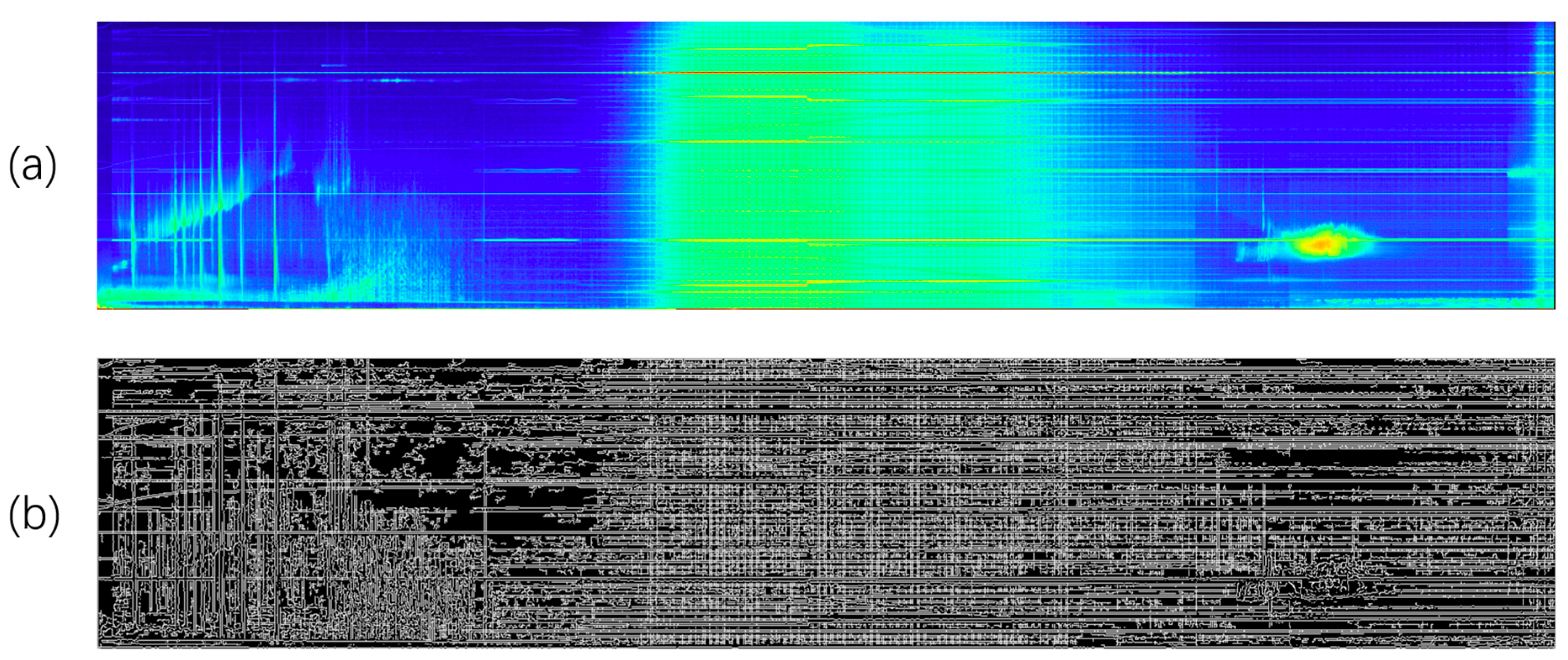
Firstly, the logarithmic operation is performed on the power spectral density data of the electric field, to solve the problem that power spectral density data usually span multiple orders of magnitude and reduce the dynamic range of the data. Then, by rotating the two-dimensional data counterclockwise by 90°, the power spectrum image can be drawn more intuitively, as shown in Figure 1. From Figure 1, it can be observed that in the X, Y, and Z direction components of the power spectrum image, the nuclear-shaped anomaly area of the Z component is more pronounced compared to the X and Y components. Therefore, the power spectrum image of the Z component is selected as the research object to create a training dataset.

The author created a total of 1115 images as the dataset, dividing the training and testing sets in an 8:2 ratio. A total of 892 images were used for model training, including 390 images of areas with nuclear-shaped anomalies and 502 images of areas without nuclear-shaped anomalies; 223 images were used for model testing, including 65 images of areas with nuclear-shaped anomalies and 158 images of areas without nuclear-shaped anomalies. For the production of pixel-level label data, the data label annotation tool used is LabelImg, which annotates the nuclear-shaped abnormal areas in the power spectrum image and generates a JSON file, which sets the pixel classification information of the image. When processing labeled data, the pixel value of the nuclear-shaped anomaly area is mapped to 1, and the pixel value of other background areas is mapped to 0. The processed label result is shown in Figure 2.

3. Detection Method for Nuclear-Shaped Anomaly Areas

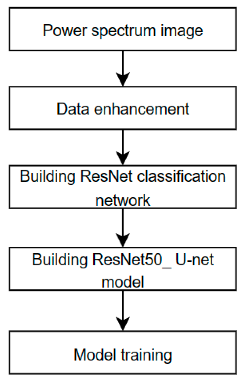
The goal of this algorithm is to achieve the detection of nuclear-shaped abnormal areas in power spectrum images. The steps are as follows: firstly, the Albumentations data augmentation library is used to enhance the power spectrum image [31]. Then, the ResNet classification network is used as the downsampling encoder of the U-net network to construct the ResNet50_Unet network model. Finally, the ResNet50_Unet model is used to train and test the dataset. The detection process is shown in Figure 3.

3.1. Data Enhancement

Data enhancement is the process of increasing the size of the training set for nuclear-shaped anomaly regions. Unlike simply copying and repeating the original data, it involves a series of random expansions and transformations on the power spectrum image to generate training samples that are different but related to the original power spectrum image.

To avoid overfitting and imbalanced samples in the model and improve the accuracy of detecting nuclear-shaped abnormal areas in the power spectrum image, the data are preprocessed from the following two aspects. One is to increase the amount of data for training the model, improve its generalization ability, and adjust the size of the original dataset image to 256 × 1024 by cropping it on the original image so that the features of the nuclear-shaped anomaly area in the original power spectrum image are unchanged. Horizontal flipping flips the power spectrum image along the vertical axis, with a flipping probability of 50% for each image; scale translation and rotation increase the diversity of samples in power spectral images through transformations such as translation, scaling, and rotation.

The second is to increase noise data and improve the robustness of the model, by adding random noise that follows a Gaussian distribution on the power spectrum image to change the appearance of the image. Random numbers that follow a Gaussian distribution will be generated based on the specified mean and standard deviation and applied to each pixel value of the image as the intensity of noise. To prevent information loss caused by excessive changes in image features, the probability of Gaussian noise data augmentation is set to 20% for each image.

The author used the Albumentations data augmentation library to enhance the power spectrum image data. In addition to the main data augmentation methods mentioned above, there are also some other data augmentation methods listed in

Table 1. Data augmentation methods.

Enhanced Mode	Enhanced Probability	Enhancement Effect
Resize	1	resize the image
HorizontalFlip	0.5	flip the image horizontally
ShiftScaleRotate	0.5	scale translation and rotation of images
GaussNoise	0.2	adding gaussian noise interference to images
CLAHE	0.9	perform histogram equalization on images
RandomBrightnessContrast	0.9	randomly apply brightness contrast to images
RandomGamma	0.9	perform random gamma affine transformation on images
Sharpen	0.9	sharpen the image
Blur	0.9	randomly blur the image
MotionBlur	0.9	apply motion blur to images
HueSaturationValue	0.9	randomly change the hue and saturation values of an image

.

3.2. ResNet

In the process of building the ResNet50_Unet model, an important part is an encoder, whose main function is to extract the nuclear-shaped abnormal areas of the power spectrum image and condense their semantic information. The commonly used encoders are various classification networks, with famous ones being the VGG series [32] and the ResNet series [33]. As the depth of the VGG network increases, it will lose sensitivity to local spatial information and details at a deeper level. For nuclear-shaped abnormal areas, it will lead to the loss of contextual information in the central area, which is not suitable for nuclear-shaped abnormal area detection tasks. Therefore, the construction of the ResNet classification network is introduced.

Traditional convolutional neural networks have an obvious flaw. As the number of network layers increases, the gradient signal gradually weakens until it disappears, resulting in training difficulty and network degradation. Gradient disappearance is the phenomenon with further iterations of backpropagation; the gradient gradually becomes smaller and approaches zero. When the gradient disappears, the gradient information obtained by the shallower layers of the network is not enough to learn effectively, which will make model training difficult or even fail. Network degradation means that as the number of network layers increases, the performance of the model decreases. To solve these two problems, He K et al. proposed the ResNet (Residual Neural Network) deep convolutional neural network architecture [21]. By introducing residual connections (including skip connections and identity mapping), the problems of gradient disappearance and network degradation in deep network training are solved. The residual connection is a skip connection introduced inside the residual block, which adds the input directly to the output of the network, so that the network can learn the residual function and form a residual path.

The ResNet series includes multiple variants such as ResNet18, ResNet34, and ResNet50. ResNet50 is a deep residual network model with 50 convolutional layers, and its residual blocks are shown in the green module (such as Resnet50-1) in Figure 4.

The ResNet50 residual block consists of two parts: the main path and the skip connection. The main path consists of three convolutional layers, each consisting of two 1 × 1 convolutions with a 3 × 3 convolution in between. Each convolutional layer is followed by a batch normalization and activation function, which is used to learn nonlinear transformations of nuclear-shaped anomaly region features. The skip connection part directly maps the input features to the output and then obtains the classification results through the activation function. If the size of the input and output does not match, an additional 1 × 1 convolutional layer is introduced for size adjustment. This design allows the network to learn the differences in nuclear-shaped abnormal regions between the input and output layers.

Skip connections allow gradients to flow directly from shallower to deeper layers, making it easier for gradients to flow through the entire network, preserving the information of the original nuclear-shaped anomaly area and avoiding information loss. In this way, after stacking 50 convolutional layers, the ResNet50 classification network is finally obtained. It performs well in tasks such as image classification, object detection, and image segmentation, and is suitable as an encoder structure for the U-net model.

3.3. U-Net Network

In recent years, deep learning research and applications have made great progress, and convolutional neural networks are an important direction of development. In the field of computer vision, breakthroughs have been made in the application of object detection, semantic segmentation, and other technologies with convolutional neural networks as the core. Traditional image segmentation methods often struggle to capture sufficient contextual information, making it difficult to effectively segment while maintaining details. The U-net model effectively solves this problem. In 2015, the U-net network model was first proposed and successfully applied in biomedical image segmentation [23]. It is a symmetrical U-shaped structure that allows the network to capture rich contextual information at different levels while preserving high-resolution features due to the high resolution of biomedical images and the need to consider both local and global features simultaneously. To achieve this goal, U-Net adopts an encoder–decoder structure, which maintains high-resolution feature information at different levels through skip connections. Skip connections allow the network to utilize both low-level and high-level features for segmentation, thereby improving the accuracy of segmentation.

3.3.1. Building Encoder–Decoder

The first is the construction of the encoder–decoder structure of U-Net, where the encoder, i.e., the downsampling part, consists of a series of convolution and pooling operations used to progressively extract the contextual features of the image and reduce the size of the feature map. The encoder part adopts the ResNet50 classification network to extract high-level semantic information from the input power spectrum image, gradually reducing the size of the feature map, and outputting a series of feature maps of different scales, each of which contains the semantic information of the input image. The decoder part, also known as the upsampling part, gradually restores the size of the feature map extracted by the encoder to the resolution of the original image through the constructed deconvolution layer, assigns corresponding category labels to each pixel, and obtains a segmentation effect of the same size as the input image.

3.3.2. Building Skip Connections

The skip connection part of U-net is implemented in the decoder by connecting the feature map in the encoder with the feature map of the corresponding level decoder, thereby achieving the fusion of low-level and high-level features. The purpose of doing this is to integrate feature information from different scales while retaining more contextual and detailed information. This helps to solve the problems of information loss and spatial accuracy in segmentation tasks and improves the performance of the network.

The U-net network structure is shown in Figure 4.

After inputting the image into the U-net network model, it first passes through the left-half encoder section, which consists of two 3 × 3 convolutional layers and a 2 × 2 max pooling layer to form a downsampling module. After four downsampling modules, it enters the right-half decoder section. The decoder section consists of a deconvolution layer and a feature map obtained by concatenating the left half of the same layer encoder, followed by two 3 × 3 convolutional layers to form an upsampling module. After four upsampling modules, a prediction result with the same size as the input image can be obtained.

The U-net model is a modification and expansion of the network architecture of the traditional image segmentation network FCN, allowing it to obtain more accurate segmentation results with very few nuclear-shaped abnormal area images. It also adds many feature channels, allowing more original power spectrum image texture information to propagate in different layers of high resolution. In addition to being widely used in the field of medical image segmentation, U-net has also achieved significant achievements in detection tasks in other fields. Its network structure is simple and effective, and its relatively small number of parameters makes it easy to train and deploy, making it very suitable for detecting nuclear-shaped anomaly regions in images.

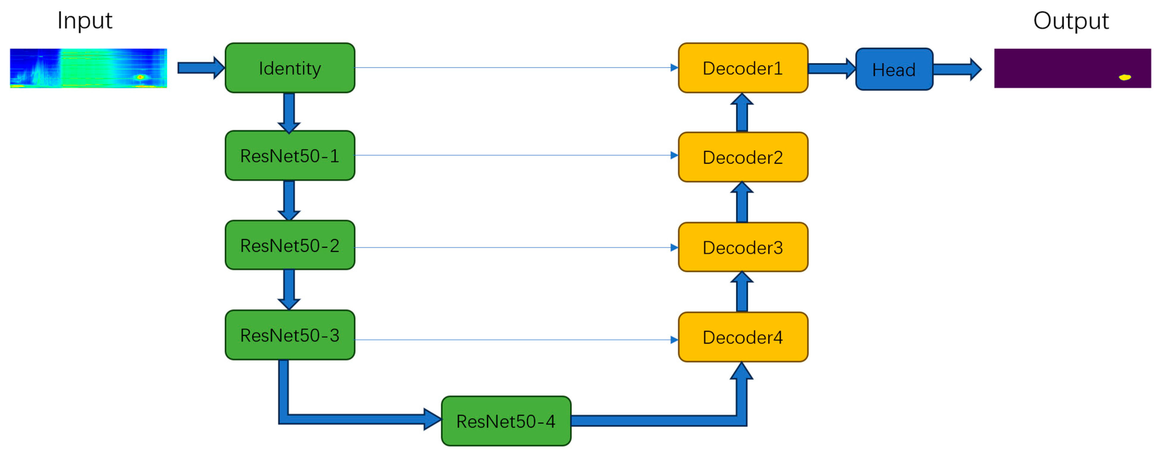
3.4. ResNet_50U-Net Network

After building the ResNet50 classification network and the original U-net network model, the encoder part of the original U-net network model is replaced by the ResNet50 classification network, where the downsampling module of the encoder is composed of ResNet50 residual blocks. The preprocessed power spectrum kernel abnormal area image is input into the model. Firstly, it enters the Identity downsampling module of the encoder to maintain the original size of the image. The channel is increased from 3 to 64, resulting in a feature map that preserves the original image features. Then, the ResNet50-1 downsampling module is entered, making the image size 64 × 256 and increasing the channel size from 64 to 256. Next, the ResNet50-2 downsampling module is entered, where the image size becomes 32 × 128 and the channel increases from 256 to 512. Then, the ResNet50-3 downsampling module is entered, the image size becomes 16 × 64, and the channel increases from 512 to 1024. Finally, entering the ResNet50-4 downsampling module, the image size becomes 8 × 32, and the channel increases from 1024 to 2048.

The encoder section is completed and enters the decoder section. Firstly, the Decoder4 upsampling module is entered to reduce the image size to 16 × 64, the feature maps of the same layer downsampling module ResNet50-3 are fused, and the channel is changed to 256. Next, the Decoder3 upsampling module is entered to reduce the image size to 32 × 128, the feature maps of the same layer downsampling module ResNet50-2 are fused, and the channel is changed to 128. Then, the Decoder2 upsampling module is entered, making the image size 64 × 256, and the feature maps of the ResNet50-1 downsampling module are fused in the same layer, making the channel 64. Then, the Decoder1 upsampling module is entered, making the image size 128 × 512, integrating the feature maps of the same layer downsampling module Identity, and changing the channel to 32. After passing through the Head module, a two-channel predicted image with the same size as the input image and containing predicted label information is obtained.

The fusion implementation process of the decoder part is as follows (taking Decoder3 as an example). Firstly, the feature map obtained by Decoder4 is enlarged by the interpolation function, and the nearest neighbor interpolation method is used to enlarge its size to the feature map obtained by Encoder ResNet50-2. Then, the feature map obtained by Encoder ResNet50-2 is connected to the enlarged feature map obtained by Decoder 4 on the channel. Finally, the feature map of Decoder3 is obtained through convolution and other operations.

The network structure of the ResNet50_U-net model is shown in Figure 4.

3.5. Loss Function

In the training process of the nuclear-shaped anomaly detection model, better measuring the difference between the predicted results and the true values of the model and guiding the updating and optimization process of the model parameters can be achieved through a loss function. The cross-entropy loss function is based on information entropy theory and is suitable for classification problems and model optimization, improving the ability to distinguish right from wrong. By taking the logarithm of the predicted probability distribution vector, multiplying it by the distribution vector of the real label, and then adding and summing the results, the difference between the predicted probability distribution output by the model and the real label is obtained. When the predicted results of the model are closer to the actual results, the cross-entropy loss is smaller, indicating better performance of the model. The formula for the cross-entropy loss function is shown in (1).

$$H(p,q)=-\sum \left[p\right(x\left)logq\right(x\left)\right]$$

(1)

Among them, $H(p,q)$ is the loss value, $p\left(x\right)$ is the probability distribution vector of the true label, $q\left(x\right)$ is the probability distribution vector predicted by the model, $\mathsf{\Sigma }$ represents the sum of all categories, and $log$ represents the natural logarithm.

To prevent overfitting issues, the weight decay strategy adopts the cosine annealing hot restart method. Weight attenuation associates the original loss function with the sum of squares of weights and adjusts the output value by adjusting the changes in weights. Its effect can make the network tend to choose smaller weight values when updating parameters, thereby reducing the complexity of the model. The loss function of weight attenuation can be expressed as Formula (2).

$$L\prime =L+\lambda \ast R\left(W\right)$$

(2)

Among them, $L\prime$ is the loss function after weight attenuation strategy, $L$ is the original loss function, $\lambda$ is the regularization coefficient used to control the intensity of weight attenuation, and $R\left(W\right)$ is the sum of squares of the weights.

3.6. Weight Attenuation Strategy

The cosine annealing hot restart weight attenuation strategy is a combination of cosine annealing and restart strategies, which can help the nuclear-shaped region detection model better converge and avoid falling into local minima. Its learning rate is adjusted according to the cosine function in each training cycle. When the learning rate drops from a larger initial value to a smaller minimum value, it will reset back to the initial value, forming a cycle. The advantage of doing this is to periodically increase the learning rate during the training process to help the model break out of local minima and continue searching for better solutions. The learning rate (loss) of the cosine annealing hot restart weight decay strategy is adjusted with the period (epoch) as shown in Figure 5.

The learning rate scheduling function for cosine annealing restart is shown in Formula (3).

$$lr=\eta \_min+0.5 \ast (\eta \_max-\eta \_min) \ast [1+cos(\pi \ast t/T\left)\right]$$

(3)

Among them, $lr$ is the learning rate of the current training cycle, $\eta \_min$ and $\eta \_max$ are the minimum and maximum values of the learning rate, $t$ is the current training cycle, and $T$ is one cycle.

After the above series of operations and processing, the intelligent detection model ResNet50_Unet for spatial electric field nuclear-shaped shape anomalies was obtained, providing a fast detection method for subsequent experiments and data processing.

4. Experimental Verification and Analysis

To verify the effectiveness of the ResNet50_Unet network in detecting nuclear-shaped anomaly areas, comparative experiments were conducted on various models using the sample set data created in the previous, including Unet++, DeepLabV3, DeepLabV3+, LinkNet, PSPNet, FPN, PAN, and Manet. In addition, experimental analysis was also conducted with some traditional methods, such as Canny edge detection, scale invariant feature transformation (SIFT), and seed region growth.

4.1. Experimental Environment

The hardware configuration is NVIDIA Tesla V100, with 32 GB of running memory, and the graphics card is GeForce RTX3090 with 24 GB of graphics memory. The software environment is the Ubuntu 18.04 operating system for Linux. To utilize the parallel computing capability of GPU and execute multiple threads simultaneously, the experiment used the parallel computing platform CUDA 11.2.1 developed by NVIDIA and the deep neural network acceleration library CUDNN 8.2.1. The deep neural network model framework was constructed and trained using Pytorch 1.9.1.

4.2. Evaluating Indicator

To objectively evaluate the performance of the model in segmenting nuclear-shaped anomaly regions, two commonly used evaluation metrics in the field of semantic segmentation were used: mean intersection over union (mIoU) and mean pixel accuracy (mPA) [21], both of which are calculated based on the confusion matrix.

The confusion matrix is based on real labels and predicted labels and classifies samples according to their classification results. For the binary image segmentation task, a confusion matrix of 2 × 2 is used, as shown in

Table 2. Confusion matrix.

	Predicted as Positive	Predicted as Negative
Actual positive class	True Positive	False Negative
Actual negative class	False Positive	True Negative

. True positive (TP): the true category of the sample is positive, and the predicted result is also positive. False negative (FN): the true category of the sample is positive, but the predicted result is negative. False positive (FP): the true category of the sample is negative, and the predicted result is positive. True negative (TN): the true negative category of the sample is negative, and the predicted result is also negative.

mIoU is the average of the intersection and union ratio between the predicted segmentation results and the true segmentation results for each class, which is the intersection of the predicted and true results divided by the union of the predicted and true results. TP/(TP + FP + FN) can be calculated using the confusion matrix, and the final average is then calculated.

mPA is the average of the pixel classification accuracy predicted by each category model. The pixel accuracy of each category can be calculated by using the confusion matrix to calculate TP/(TP + FP + FN), and finally, the average value is calculated. The value range of these two evaluation indicators is between 0 and 1, and the larger the value, the better the segmentation effect. The calculation formulas for mIoU and mPA are shown in (4) and (5).

$$mIoU=\frac{1}{k+1}\sum _{I=0}^k\frac{p_{ii}}{\sum _{J=0}^k{p}_{ij}+\sum _{j=0}^k{p}_{ji}-p_{ii}}$$

(4)

$$mPA=\frac{\sum _{i=0}^k{p}_{ii}}{\sum _{i=0}^k\sum _{j=0}^k{p}_{ij}}$$

(5)

where $k$ represents the number of target categories that need to be classified, $k+1$ represents the total number of categories plus the background class, $i$ represents the actual pixel value, and $j$ represents the pixel value predicted by the model. $p_{ij}$ represents predicting $i$ as the value of $j$, $p_{ji}$ represents predicting $j$ as the value of $i$, and $p_{ii}$ represents predicting $i$ as the correct predicted value of $i$, that is, the pixel value is equal to the true value.

4.3. Parameter Settings

To obtain better semantic segmentation results, it is necessary to optimize the parameters of the nuclear-shaped anomaly detection model. After multiple cross-validations and adjustments, the ResNet50_Unet network model parameter settings suitable for nuclear-shaped anomaly areas are listed in

Table 3. Parameter settings.

Parameter	Parameter Values
classes	2
epoch	600
batch_Size	32
optimizer	Adam
activation function	Relu
learning_Rate	0.001

.

The model optimizer uses Adam (Adaptive Moment Estimation) to dynamically adjust the learning rate based on the first-order moment estimation of the gradient (i.e., the mean of the gradient) and the second-order moment estimation (i.e., the variance of the gradient). The training set batch_Size = 32, the test set batch_Size = 16, epoch = 600, and the activation function is Relu (Rectified Linear Unit). It is a nonlinear function that can introduce nonlinear characteristics and has advantages such as high computational efficiency, avoiding gradient vanishing, and sparse activation. The initial learning is 0.001, and the weight decay strategy method adopts the cosine annealing hot restart method. When the epoch reaches 20, the learning_Rate is reset to 0.001, and then the learning rate is dynamically adjusted based on the convergence result until the best evaluation indicator, such as mIoU or mPA, reaches the maximum value, or the epoch reaches the set value, which ends the training.

4.4. Comparison of Traditional Methods

For the detection task of nuclear-shaped abnormal areas, in addition to supervised deep learning, traditional methods are also used to detect nuclear-shaped abnormal areas. It is mainly divided into two parts, traditional edge-based detection methods (Canny edge detection and SIFT) and region-based detection methods (seed region growing). The following is an analysis of the experimental results of using traditional methods to detect nuclear-shaped anomaly areas.

Firstly, experimental analysis will be conducted on the Canny edge detection method. The commonly used operators for edge detection include the Canny operator, Sobel operator, Laplace operator, etc. After comparative experiments, the Canny operator with relatively better performance is selected for comparative experiments. The results obtained through Canny edge detection are shown in Figure 6b, indicating that the edges of the nuclear-shaped anomaly area were not detected.

Experimental analysis was then conducted on the sift detection method. Its advantages lie in image scale invariance, rotation invariance, and lighting invariance, which can extract the same feature points regardless of whether the image is captured at close or long distances, or through rotation and tilt transformations. However, due to the fact that power spectrum images rarely exhibit the aforementioned situations, the advantages of the SIFT method are not well demonstrated. The detected key points are shown in Figure 7b, and it can be seen that the detected key point information is not unique to the nuclear-shaped anomaly area.

The experimental analysis of the seed region growth detection method based on region is as follows. Due to the fact that the nuclear-shaped anomaly area is not in a fixed position, considering efficiency issues, the initial seed is set to be automatically selected. Given the need for nuclear-shaped anomaly detection tasks, the growth criterion is set to be that the Euclidean distance between pixel values is less than a certain threshold, which means that when the difference between adjacent pixel values is small, it is classified as a region. Due to the darker color of the nuclear-shaped anomaly area, it can be separated. The detected nuclear-shaped abnormal area is shown in Figure 8b, and it can be seen that the nuclear-shaped abnormal area has not been well detected.

After the above experimental analysis, it was found that traditional methods are not ideal for detecting nuclear-shaped anomalies.

4.5. Comparative Experiment

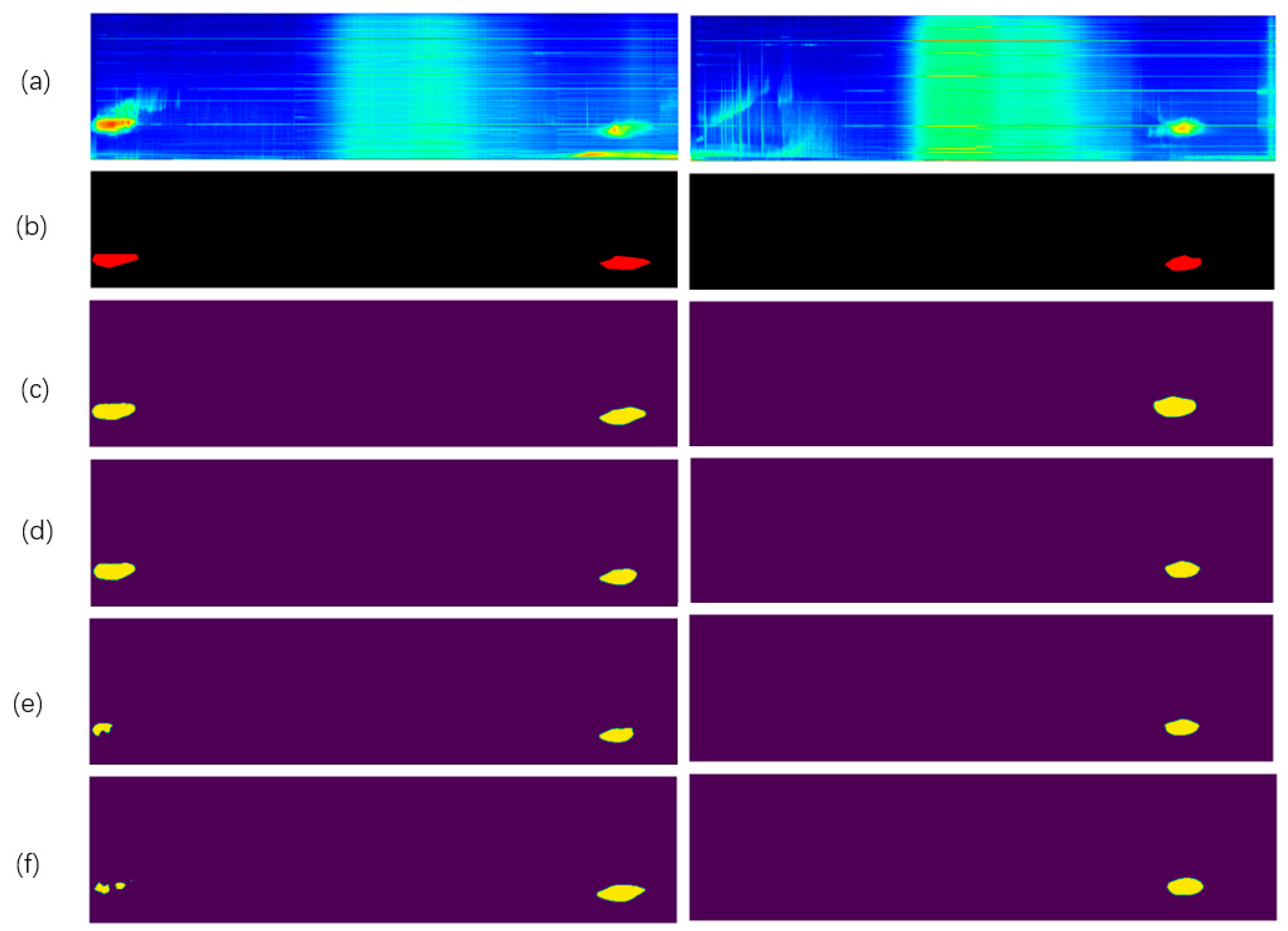
To evaluate the effectiveness of different models, two comparative experiments were conducted using the sample set created in the previous section. The first group of experiments compares the segmentation performance of the ResNet50_Unet model with eight popular semantic segmentation algorithms. The second group of experiments compares the segmentation performance of different encoder networks at an epoch of 200. The comparison results of the image segmentation algorithms in the first comparative experiment are listed in

Table 4. Comparison results of image segmentation algorithms.

Model	mIoU	mPA
ResNet50_Unet	0.741681	0.998994
DeepLabv3	0.718519	0.998905
PSPNet	0.685374	0.998711
LinkNet	0.716289	0.998867
FPN	0.708899	0.998785
DeepLabv3+	0.720010	0.998965
Unet++	0.700127	0.998845
PAN	0.707727	0.998922
MAnet	0.716172	0.998954

, and some predicted results are visualized in Figure 9. It can be seen that both evaluation indicators of the ResNet50_Unet model are the best. From Figure 9, it can be seen that the ResNet50_Unet model has good segmentation performance and superior performance. The segmentation results of the second comparative experiment are listed in

Table 5. Comparison results of different encoders.

Encoder	mIoU
VGG11	0.654
VGG13	0.676
VGG16	0.696
ResNet18	0.678
ResNet34	0.713
ResNet50	0.741

, and the visualization of their prediction results is shown in Figure 10. It can be seen that the ResNet50 encoder has the best performance.

At the same time, there are also some cases of unsuccessful detection, such as the left half of subgraphs e and f in Figure 9, where the nuclear-shaped anomaly area on the left side of the image is not well detected. Just detecting the area with the highest energy value cannot include the entire nuclear-shaped anomaly area. This may be due to the model not taking into account the global features of the nuclear-shaped anomaly area during segmentation, resulting in missing feature maps and unsuccessful detection.

5. Discussion

Due to the first observation of the location of the nuclear-shaped anomaly area on 14 December 2021, to further analyze the frequency distribution, global spatial distribution, and magnetic latitude distribution of the nuclear-shaped anomaly area, this article takes the time at which the nuclear-shaped anomaly area was first observed (14 December 2021) as the central time point, advances by one month and increases the data by the next two months (November 2021 to February 2022) for a total of four months as the research object; 93 orbits (including ascending and descending orbits) were found to have 101 nuclear-shaped anomaly areas, covering the entire world.

5.1. Frequency Distribution

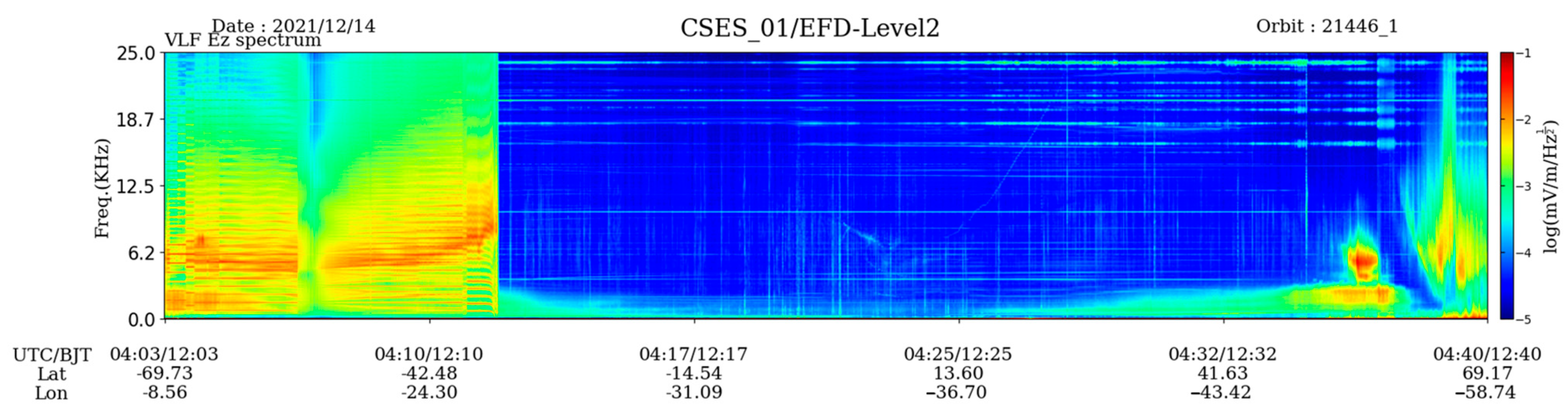
Statistical analysis shows that the frequency of the nuclear-shaped anomaly area is mostly between 0 and 12.5 kHz, mainly concentrated around 6 kHz, with only one anomaly occurring at 16 kHz. The starting position of this abnormal area is at 164.06° W and 50.42° S, and the ending position is at 165.56° W and 53.1° S, with the highest energy value located at 164.96° W and 52.03° S, crossing longitude and latitude of 1.5° and 2.68°, respectively, as shown in the red circle area in Figure 11.

5.2. Global Spatial Distribution

Analyzing the spatial locations of all 101 nuclear-shaped anomaly areas in the four-month data, it was found that they were distributed between 40° and 70° in the south and north latitudes, including 55 in the north latitude area and 46 in the south latitude area, as shown in Figure 12. Among them, there are 37 between 60° and 70° north latitude, accounting for 67%, while there are only 6 between 60° and 70° south latitude, less than 13%.

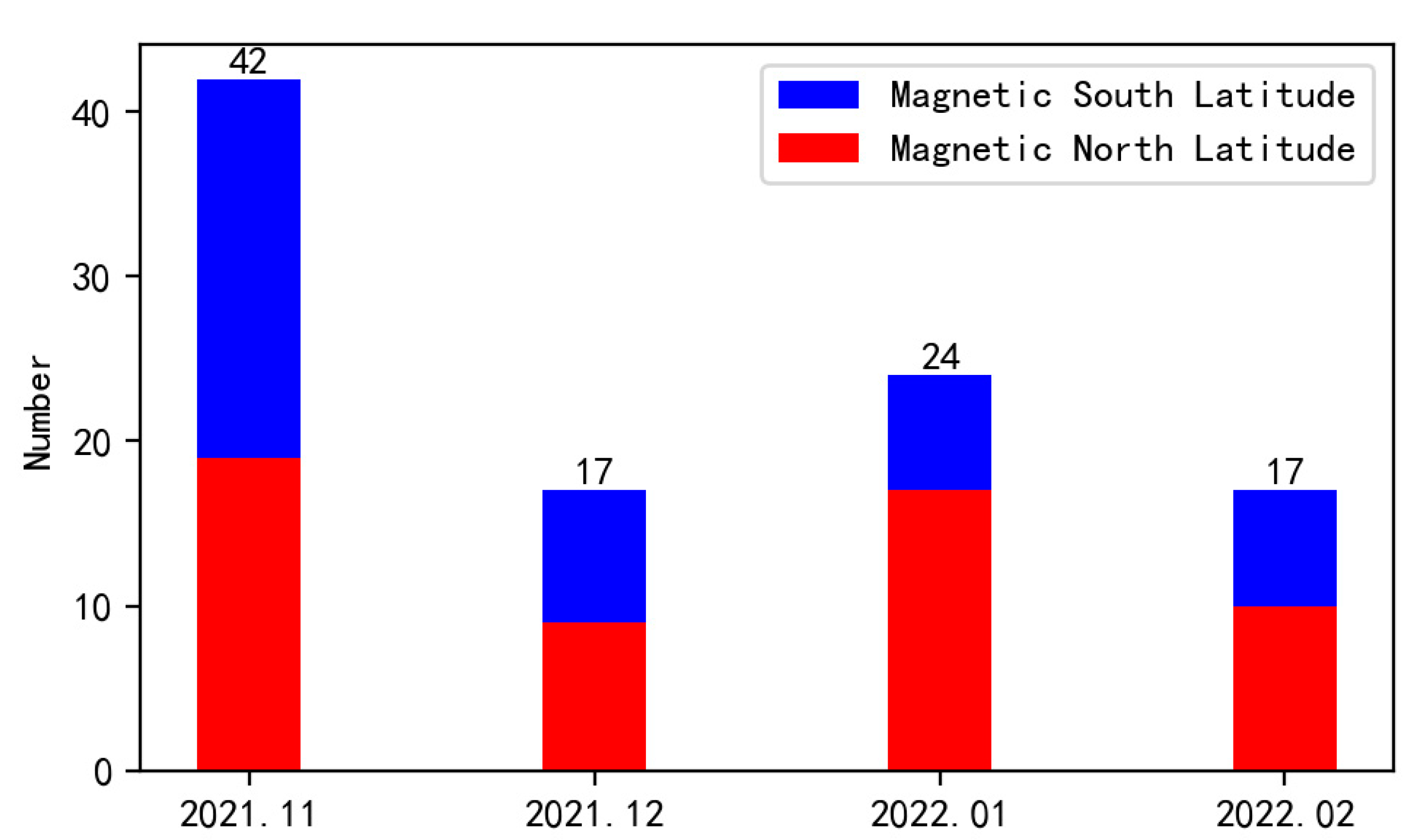
The number of nuclear-shaped abnormal areas in each month from November 2021 to February 2022 is 43, 17, 24, and 17, respectively. The line chart of their number distribution is shown in Figure 13. It can be seen from the figure that the number of nuclear-shaped anomaly areas in November is significantly greater than that in the other three months, and there are more areas in southern latitudes than in northern latitudes, which may be due to seasonal factors. The specific reasons are not yet clear, and further research can explore seasonal factors. The following is a further analysis of the global spatial distribution of each month during the selected research period.

A study on the global spatial distribution of nuclear-shaped anomaly areas was conducted in November 2021. A total of 43 abnormal areas were found, including 19 in northern latitudes and 23 in southern latitudes, as shown by the orange dots in Figure 13. In the northern-latitude region, there are 9 between 40° and 60°, while the remaining 10 are between 60° and 70°. In the southern-latitude region, 21 are found between 40° and 60°, and the remaining 2 are between 60° and 70°.

Further analysis of the global spatial distribution of nuclear-shaped anomalies in December 2021 revealed 17 anomalous regions, including 9 in the north latitude region and 8 in the south latitude region, as shown by the green dots in Figure 13. In the northern-latitude region, only one is located between 40° and 60°, while the other eight are between 60° and 70°. In the southern-latitude region, there are a total of six between 40° and 60°, and only two are found between 60° and 70°.

An analysis of the global spatial distribution of nuclear-shaped anomalies in January 2022 revealed 24 anomalous regions, including 17 in the north-latitude region and 7 in the south-latitude region, as shown by the blue dots in Figure 13. In the northern-latitude region, 3 were found to be located between 40° and 60°, while the other 14 were found to be between 60° and 70°. In the southern-latitude region, all were located between 40° and 60°, and no nuclear-shaped anomalies were found between 60° and 70°.

The global spatial distribution of nuclear-shaped anomalies in February 2022 was analyzed. A total of 17 abnormal regions were found, including 10 in the north-latitude region and 7 in the south-latitude region, as shown by the purple dots in Figure 13. In the northern-latitude region, 5 were found between 40° and 60°, while the remaining 5 were found between 60° and 70°. In the southern-latitude region, 6 were found between 40° and 60°, and the remaining 1 was found between 60° and 70°.

5.3. Magnetic Latitude Distribution

Statistical analysis was performed on the distribution of magnetic latitudes in the nuclear-shaped anomaly area of the research object’s four-month data. Due to the similarity between the division of magnetic latitude and geographical latitude, the number of statistics in the north–south direction remains unchanged. The statistical histogram is shown in Figure 14.

The statistical analysis of global magnetic latitude distribution in nuclear-shaped anomaly areas is as follows. The vast majority of nuclear-shaped anomaly areas are distributed between 60° and 80° of the north–south magnetic latitude, as shown in Figure 15. The orange, green, blue, and purple dots in the figure represent the nuclear-shaped anomaly areas in November, December, January, and February, respectively. Only three cases are located above 80° in the northern magnetic latitude region, with one case in December, one case in January, and one case in February, while the rest are all located between 60° and 80°. In the southern magnetic latitude region, only four cases are located above 80° and all are in December, two cases are located below 40° and also in December, and the rest are all between 60° and 80°.

The fact that the energy in the nuclear-shaped anomaly area is stronger at the center and weaker at the edges has a significant impact on the accuracy of model detection. Therefore, further research will be conducted in the following three aspects.

(1)

Based on existing network models, algorithm improvements and optimizations are carried out to make the model more suitable for detecting nuclear-shaped anomaly areas and improving detection accuracy.

(2)

Based on the detection of nuclear-shaped abnormal areas, the detection of abnormal areas for other signals is researched and expanded.

(3)

On the basis of existing research on the global spatial distribution, the impact of seasonal factors on the global spatial distribution of nuclear-shaped anomaly regions is explored.

Based on the above analysis of the frequency distribution, global spatial distribution, and magnetic latitude distribution of nuclear-shaped anomaly areas, the possible physical process for their generation is due to changes in the magnetic field and spatial position, which cause anomalies in waveform data and power spectral density data, resulting in the appearance of nuclear-shaped anomaly areas in the power spectral image.

6. Conclusions

There are some nuclear-shaped anomaly areas in the power spectrum image of the VLF frequency band of the space electric field, with varying sizes and positions, and the formation mechanism is unknown, which is a scientific problem worthy of in-depth research. This paper is based on the power spectrum image data of the CSES-01 electric field. By constructing a ResNet50_Unet network model, the detection of nuclear-shaped anomaly areas is achieved. The nuclear-shaped anomaly areas from November 2021 to February 2022 are taken as the research object, and their frequency and spatial distribution information are further analyzed. The conclusions are as follows:

(1)

The ResNet50_U-net network model can quickly detect nuclear-shaped anomaly areas in the VLF frequency band power spectrum images of space electric fields, providing reference value for detecting ionospheric spatial anomaly disturbances through CSES-01 power spectrum images.

(2)

The energy value of the nuclear-shaped anomaly area diverges and weakens from the center to the periphery, with a frequency distribution mainly concentrated around 6 kHz. The global spatial distribution is between 40 and 70° south and north latitude, and the northern hemisphere is more than the southern hemisphere. This information provides basic support for the study of the causes, physical mechanisms, and impacts of the formation of nuclear-shaped anomaly areas.

(3)

The application of the ResNet50_U-net network model provides a reference for semantic segmentation technology in detecting other types of spatial electromagnetic field disturbances and lays the foundation for subsequent research on nuclear-shaped anomaly areas.