Annual Daily Irradiance Analysis of Clusters in Mexico by Machine Learning Algorithms

Abstract

The assessment of solar resources involves the utilization of physical or satellite models for the determination of solar radiation on the Earth’s surface. However, a critical aspect of model validation necessitates comparisons against ground-truth measurements obtained from surface radiometers. Given the inherent challenges associated with establishing and maintaining solar radiation measurement networks—characterized by their expense, logistical complexities, limited station availability and the imperative consideration of climatic criteria for siting—countries endowed with substantial climatic diversity face difficulties in station placement. In this investigation, the measurements of annual solar irradiation, from meteorological stations of the National Weather Service in Mexico, were compared in different regions clustered by similarities in altitude, TL Linke, albedo and cloudiness index derived from satellite images; the main objective is to find the best ratio of annual solar irradiation in a set of clusters. Employing machine learning algorithms, this research endeavors to identify the most suitable model for predicting the ratio of annual solar irradiation and to determine the optimal number of clusters. The findings underscore the efficacy of the L-method as a robust technique for regionalization. Notably, the cloudiness index emerges as a pivotal feature, with the Random Forest algorithm yielding superior performance with a R² score of 0.94, clustering Mexico into 17 regions.

1. Introduction

Planning the strategic locations for the installation of a comprehensive measurement network proves to be indispensable for the assessment of solar resources, especially in vast territories characterized by a multitude of climatic variations [1,2]. The substantial financial commitment entailed in establishing solar radiation measurement stations, coupled with the inherent challenges associated with their sustained maintenance, underscores the critical need for methodological approaches capable of precisely determining both the optimal number of stations and the most suitable deployment sites [3]. To address this imperative, recent years have witnessed the publication of several works that delve into the identification of potential sites for solarimetric station installations, leveraging advanced techniques such as data mining and cluster analysis [1,2,4]. These methodological advancements not only contribute to the refinement of the selection process, but also pave the way for enhanced resource assessment methodologies, ensuring a more robust foundation for solar energy planning and utilization. In light of the dynamic nature of climate patterns and the evolving landscape of renewable energy research, the continued exploration and refinement of these methodologies are essential for sustaining the accuracy and relevance of solar resource assessments in the face of changing environmental conditions.

However, the application of machine learning techniques, as evidenced in the existing literature, is not limited solely to site identification; it encompasses a multifaceted array of capabilities extending well beyond this fundamental aspect. Chief among these applications is the prediction of solar irradiation at the surface, a task accomplished through the implementation of sophisticated neural-fuzzy models, machine learning algorithms and various artificial intelligence methodologies [5,6,7]. This broad and diversified spectrum of applications highlights the versatility of machine learning within the realm of solar resource assessment research.

As the field progresses, the integration of these advanced techniques holds the promise of significantly enhancing the overall efficiency of measurement networks deployed across diverse geographic climates. Beyond the traditional role of site selection, machine learning stands poised to revolutionize the precision and reliability of solar irradiation predictions. Such advancements not only contribute to a more accurate understanding of solar energy potential, but also hold the potential to optimize the operational performance of solar energy systems. The continuous evolution and refinement of machine learning methodologies in solar resource assessment are pivotal for ensuring the resilience and adaptability of renewable energy strategies in the face of dynamic environmental conditions and emerging technological developments.

Machine learning has been applied in order to forecast solar radiation through a time series of multiple related features [8,9,10,11]. The first regionalization works for monitoring solar radiation, based on cluster analysis techniques using cloud cover data and satellite images, were carried out by Zagouras in 2013 [12]. This approach involves dividing a geographical region into a set of k clusters as a method to analyze solar irradiation patterns across the specified area. Other regionalization studies can be seen in the works of Journée in 2012 and Lima in 2016 [13,14]. In these studies, the Netherlands was regionalized [13], and Brazil [14]. In these works, Global Horizontal Irradiance (GHI) was analyzed using satellite images as well as measurements obtained from solar measurement stations, applying algorithms such as K-means and Ward; k-means is the most commonly used algorithm in cluster analysis, in which the algorithm is applied to satellite images, given a set x = {x₁, x₂, x₃, …, x_n} of n data points (pixels), and k classes a priori; the algorithm randomly places the k centroids C = {c₁, c₂, c₃, …, c_k} in the initial space and assigns the data to one of the classes based on the shortest distance between the data point and the centroid; and the goal is to minimize the differences within each group and maximize the differences between the classes. The results of the above studies led to the grouping of four classes, both in Brazil and in the Netherlands.

As can be observed, most regionalization works are based on direct measurements of solar radiation through time series, and very few have employed geoclimatic variables. The cluster analysis, segments the solar irradiation in different regions according to a similarity criterion and k number of clusters. The data used are taken mostly from time series in satellite images and ground-based measurements, and for validation and determination the appropriate number of clusters is evaluated by internal validation methods that consider the intrinsic information of the geometrical structure of the data, such as the Silhouette Index (SI) [15], Davies–Bouldin (DB) and Calinski–Harabasz indexes, with the help of the L-method [12,16]. The first index is a highly complex calculation that is difficult to evaluate in special resolutions like Mexico, and the L-method seems to be a good method for obtaining an optimal number of classes. In 2014, a regionalization was published, for the case of Mexico, based on climatic parameters such as isotherms, isohyets, evaporation and humidity to locate the stations of a solarimetric network in Mexico [4]. The presented literature underscores the evident underutilization and recent exploration of the clustering technique in the context of regionalization based on solar irradiation, employing diverse climate parameters and satellite imagery. Notably, investigations in this domain have primarily focused on a limited scope, with studies leveraging satellite images predominantly emphasizing a singular variable: cloudiness.

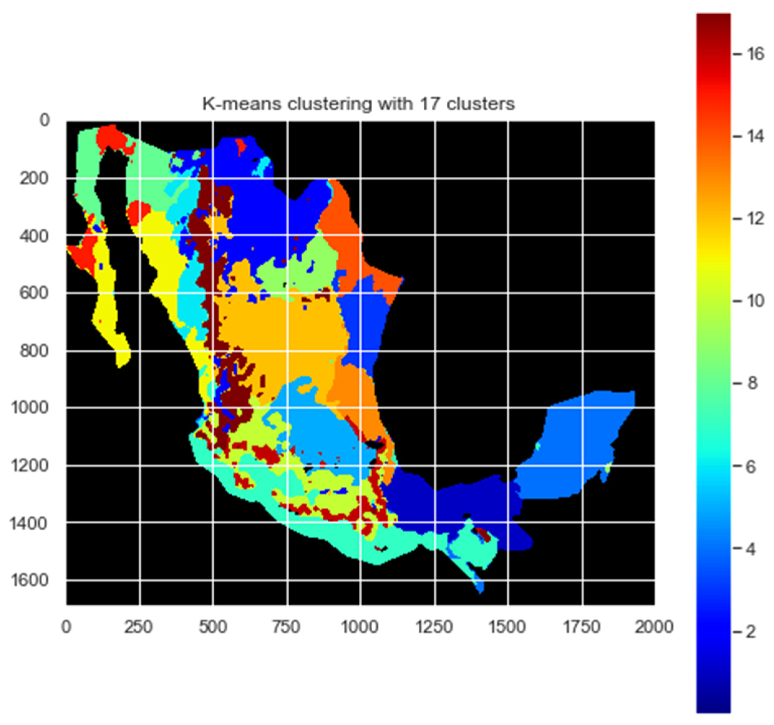
A work was recently published that performs regionalization based on solar irradiation, measuring different climatic characteristics such as albedo, cloud cover, altitude and atmospheric turbidity [1]. In this research, regionalization is accomplished through the application of the unsupervised K-means classification method and Gaussian models. Consequently, multiple regionalizations (clusters) were obtained, and internal validation methods such as DB and CH were used, applying the L-method for clustering in Mexico using satellite images of cloudiness index, albedo, Linke and altitude, and determining the option of 17 regions as the optimal regionalization. In this context, the above results showed that it is possible to find optimal regionalization through the clustering methods applied. However, recent studies show that there are different machine learning methods that can also help to forecast and estimate solar radiation.

The principal aim of this paper is to broaden the analytical scope beyond the initial exploration of k clusters. Central to this objective is the integration of additional machine learning algorithms, marking a deliberate expansion of the study’s methodological framework. This involves statistical regionalization based on parameters relevant to solar radiation incidence on the Earth’s surface. These parameters include elevation, which correlates solar radiation with the optical path length of the atmosphere; albedo, which is related to the radiation reflected by the surface and influences the amount of diffuse radiation in the atmosphere; cloud cover, which filters extraterrestrial direct radiation reaching the Earth through absorption, reflection and scattering; and atmospheric turbidity, linked to the scattering and attenuation of solar radiation by locally present particles and gasses in each region. Due to the volume of information, big data techniques are employed. These same techniques allow for the calculation of the significance of these parameters in relation to measurements from surface solar radiation stations. Notably, the study delves into the application of diverse methodologies, including Random Forest (RF), Artificial Neural Networks (ANN), Support Vector Machines (SVM) and Multiple Linear Regression (MLR), derived from the bases established in [1], and secondly works to identify the machine learning algorithm that presents the best model to forecast and estimate solar irradiance. To achieve the above, the annual daily irradiation from 26 meteorological stations were localized in each cluster, averaged and then related to the cluster’s centers of each k cluster. The results of this paper concluded that the L-method is a good method to perform regionalization since it coincides with the machine learning algorithms in this work; all the models show that 17 clusters is the optimal regionalization when solar irradiance and climatic variables are related. The results also show that the Random Forest Algorithm gives the best model, with an R² correlation score of 0.94 in the regionalization of 17 clusters. This alignment between the L method and machine learning algorithms serves as a valuable insight, emphasizing the importance of methodological coherence in achieving accurate and consistent regionalization results. The congruence observed in this study contributes to the evolution of optimal regionalization approaches and their alignment with machine learning methodologies.

2. Materials and Methods

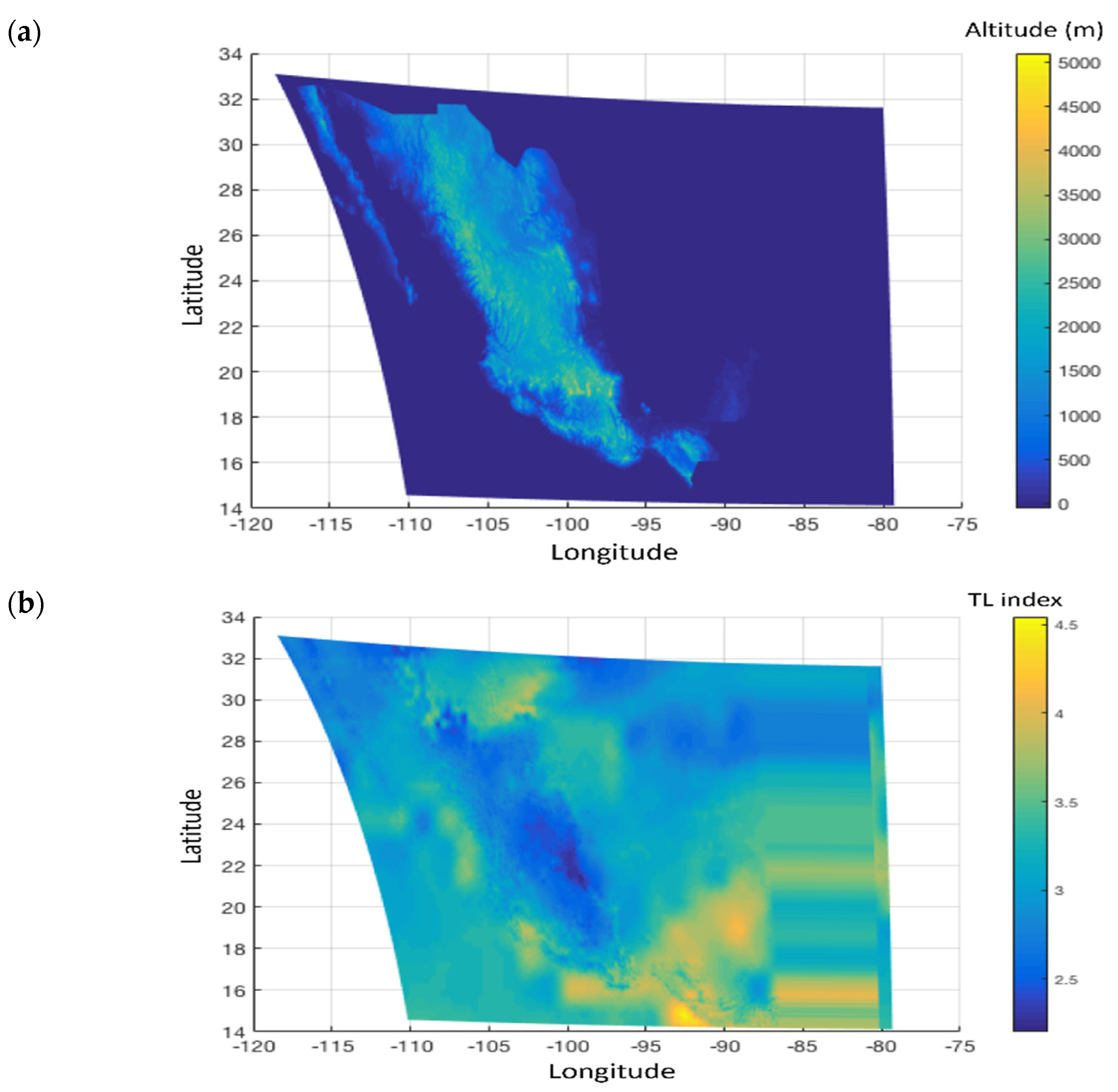
The creation of the dataset used is discussed in [1], wherein detailed explanations are provided regarding the preprocessing, modeling and evaluation of satellite images. This process resulted in the generation of datasets and maps that cluster Mexico into distinct regions based on annual values of albedo, Linke, cloudiness index and altitude for the year 2015. It must be noted that albedo and cloudiness index were obtained with the visible band of satellite GOES13 and using the methodology for Heliosat-2 [1]. In this methodology, Heliosat-2 estimates the fraction of clear sky measuring the reflectance of solar radiation by the Earth’s surface and clouds. Minimum values on the surface represent the Earth’s albedo and higher reflectance represents the cloudiness index. The Linke turbidity index was obtained from solar radiation data (SoDa services), and altitude was obtained from the National Institute of Statistics and Geography of Mexico (Figure 1).

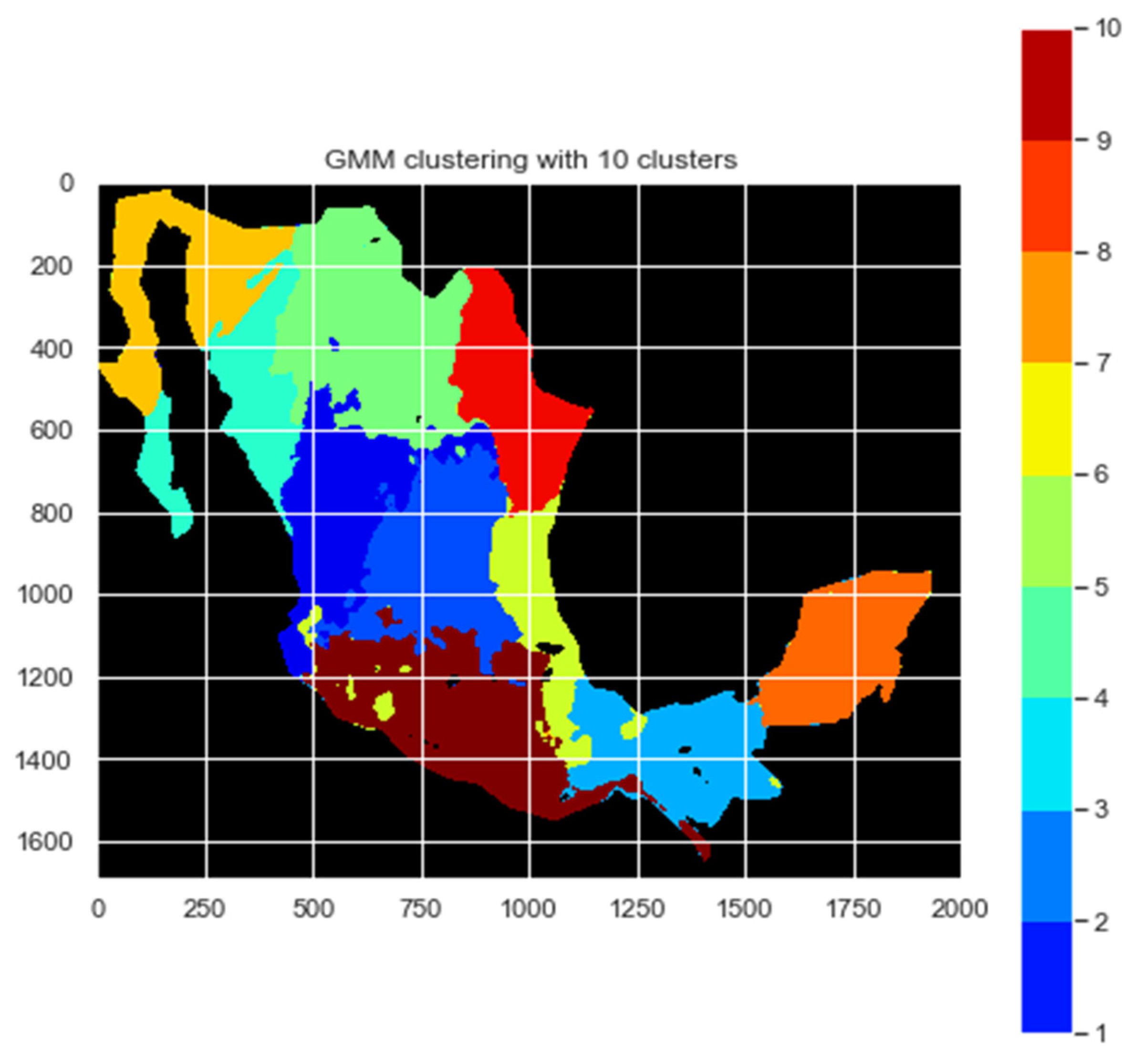
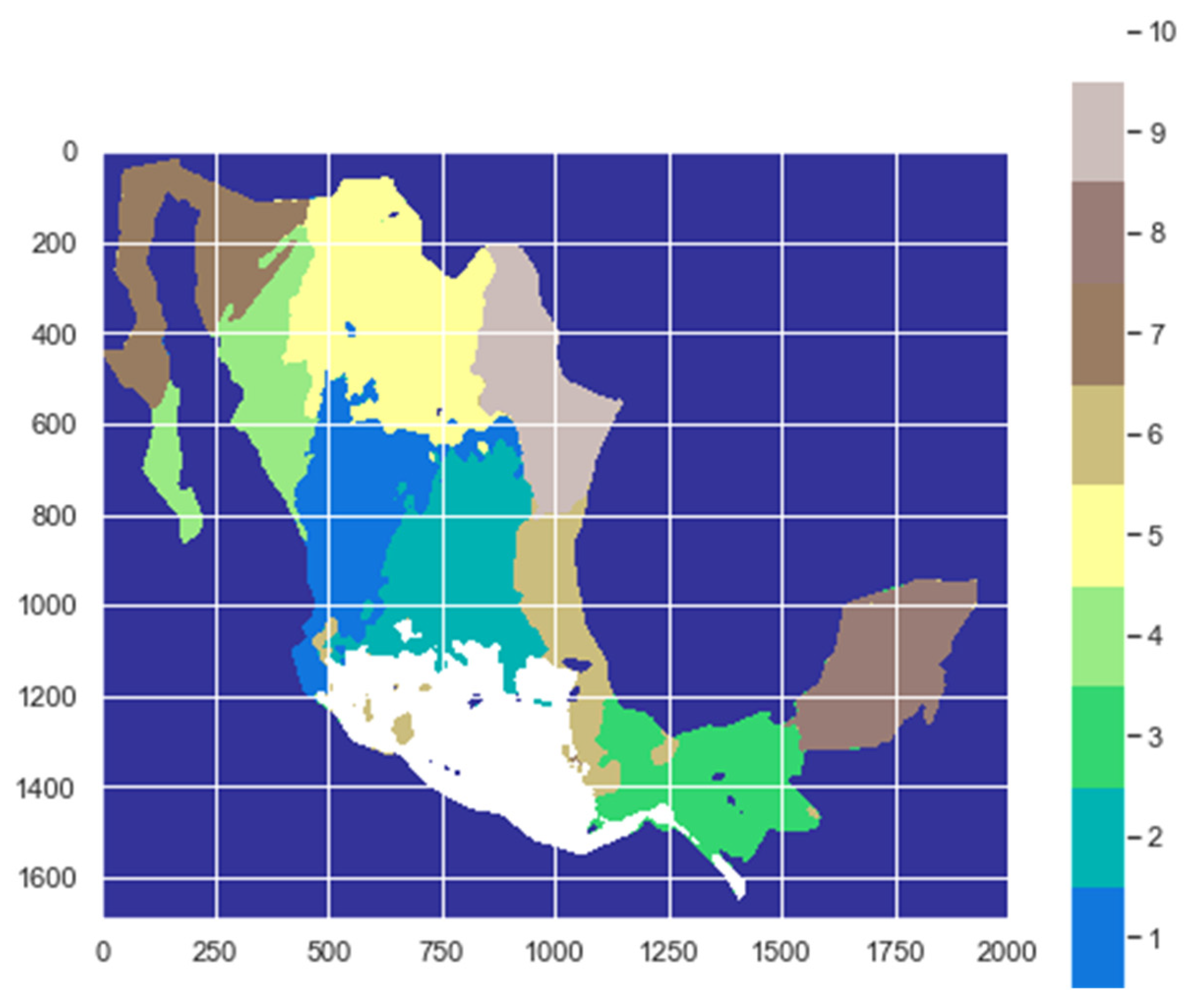
The dataset of this study contains the following columns: evaluation, class, annual daily irradiation, albedo center, Linke center, cloudiness index center and altitude center. The evaluation describes the index with the clustering method, such as K-means and Gaussian Mixture Models (GMM), and the numbers of k clusters used; for example, GMM10 means that the following 10 rows are from a cluster analysis in which the GMM algorithm was applied. The class indicates through a number the cluster class or region; for example, in Figure 2, class 3 is the region in light blue.

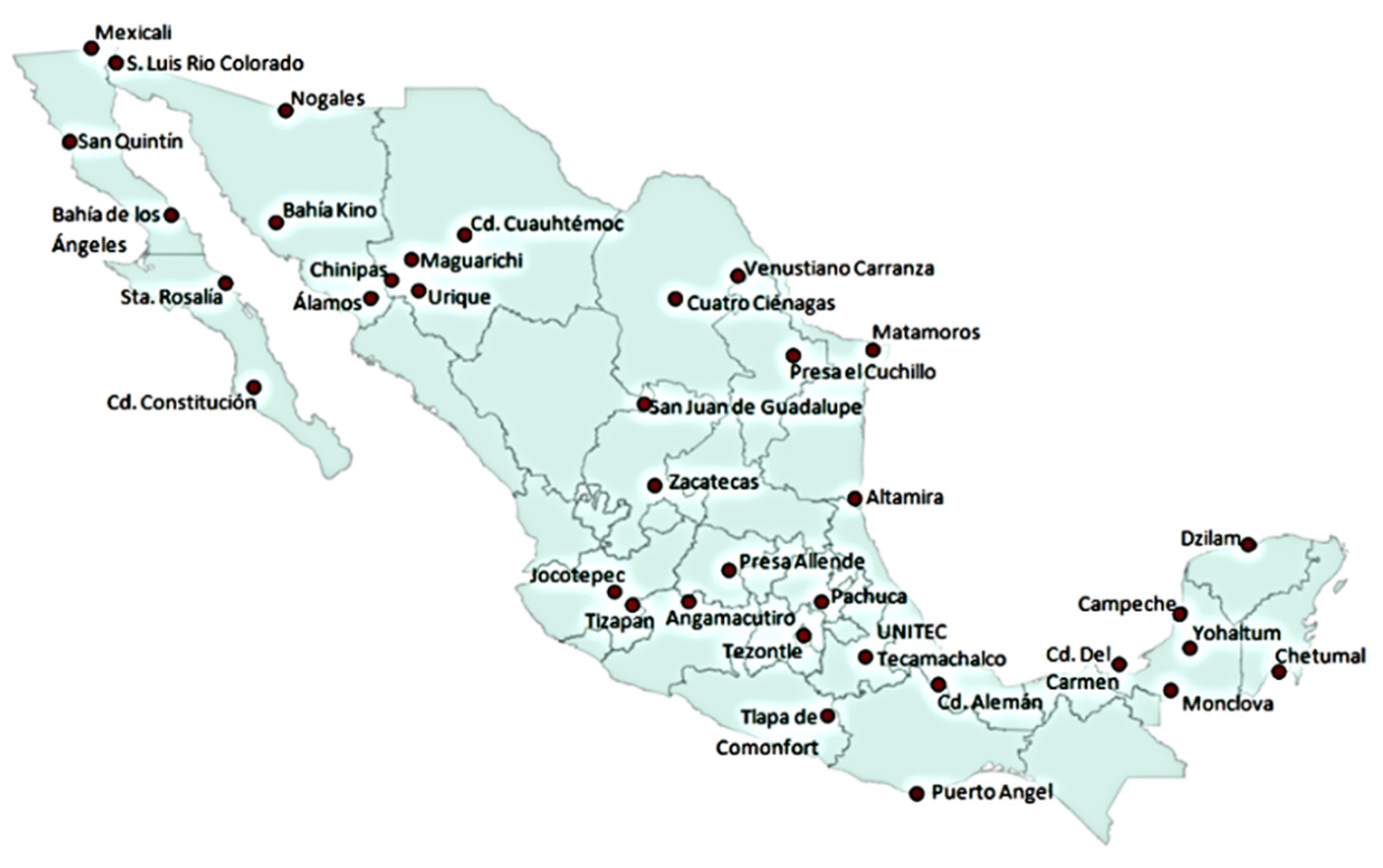
The annual daily irradiation of each class was taken by 26 ground-based stations of the National Weather Service of Mexico (SMN) (Figure 3).

The dataset utilized in this study provides meteorological data and global solar irradiance measurements obtained through thermopile pyranometers manufactured by Kipp and Zonen^® (Delft, Netherlands) and Campbell Scientific^® dataloggers (Logan, UT, USA) [3]. The geographical coordinates for each station are listed in

Table 1. Station names and their geographical coordinates.

Number	Station Name	Lat.	Lon.	Altitude [m]
1	Nevado de Toluca	19.12	99.77	4139
2	Altzomonil	19.11	98.65	4007
3	Matías Romero	16.882	95.03	186
4	Nueva Rosita	27.92	101.33	366
5	Centla	18.4	92.64	3
6	Ixta-Popo	19.09	98.64	3682
7	Agustín Melgar	25.26	104	1226
8	Monclova	18.05	90.82	100
9	Oxkutzcab	20.29	89.39	28
10	Acaponeta	22.46	105.38	29
11	Paraíso	18.42	93.15	4
12	Obispo	24.25	107.18	4
13	Petacalco	17.98	102.12	53
14	Atlacomulco	197.991	98.87	2570
15	Maguarich	27.85	107.99	1663
16	Atoyac	17.2	100.44	120
17	Ocampo	28.82	102.52	1663
18	Perote	19.545	97.26	2410
19	Miahuatlán	16.34	96.579	1588
20	Nochistlán	17.43	97.24	2040
21	Matehuala	23.64	100.65	1627
22	Mexicali	32.66	115.29	14
23	Apatzingán	19.082	102.37	282
24	Angamacutiro	20.12	101.72	1730
25	Presa Abelard	32.44	116.91	156
26	Nogales	31.29	110.91	1269

.

The acquisition of irradiance data was conducted with measurements registered every 10 min. To maintain temporal consistency with the other features, taken from the year 2015, the same was applied to these data. The daily global irradiation was obtained in Watts-hour units using Equation (1), where $I_{G_d}$ is the daily irradiation per day and Nd is the amount of data per day.

$$I_{G_d}={\displaystyle \sum }_{n=1}^{Nd}\frac{I_{G_n}}{6}$$

(1)

To obtain the annual daily irradiation $I_{G_y}$, the data were averaged, as is observed in Equation (2), where Ny is the number of days studied.

$$I_{G_y}=\frac{{{\displaystyle \sum }}_{n=1}^{N_y}{I}_{G_{d_n}}}{Ny}$$

(2)

The annual daily irradiation of each station was located in the regions for each test, and if a class had two or more pieces of data, then the annual daily irradiation of this class was averaged; the result was a sorted vector called $y_{stations}$ and contained the annual daily irradiation of the classes of each test, so for example in a regionalization of 10 classes, there are 10 sorted annual daily irradiation data.

The albedo, Linke, cloudiness index and altitude centers are the annual averages of their measurements for each class; the data were taken by the centroids of each class. The ground-based measurements and the satellite images were taken from datasets that belonged to the Institute of Geophysics at the National Autonomous University of Mexico (UNAM) (For any clarification or requests for using the data, they can be requested from the following url: https://solarimetrico.geofisica.unam.mx (accessed on 5 February 2024)).

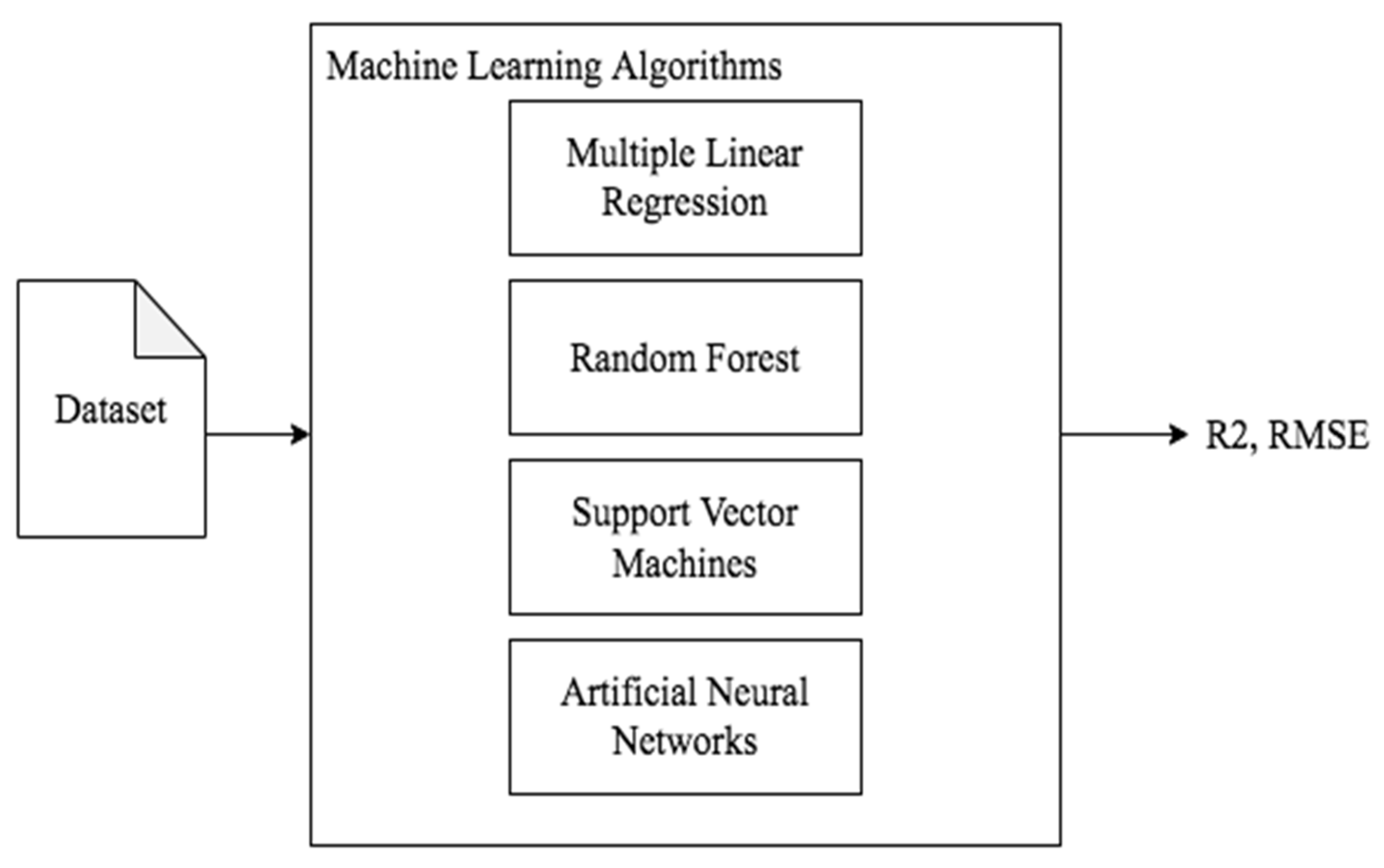
The diagram in Figure 4 shows the employed methodology: the dataset is used as an input for modeling each machine learning algorithm, and then the models are evaluated, and the outputs are the Root Mean Square Error (RMSE) and R² score of each evaluation.

In the subsequent subsections, a detailed description of the machine learning algorithms used in this study is presented.

2.1. Multiple Linear Regression (MLR)

The MLR is an extension of simple linear regression, and the aim of this algorithm is to find the values of beta coefficients that minimize the prediction error of a linear equation. Even though a linear dependence is not expected between irradiance and the considered parameters in terms of physical processes, the value of the coefficients can provide an estimation of the relative importance of each of the parameters used in relation to the magnitude of irradiance. The multiple linear regression follows Equation (3), where $y_{stations}$ is the annual daily irradiation data, $\beta$ are the coefficients of each x’s values for each i feature (independent variables such as albedo, cloudiness index, Linke and altitude) and an error term is denoted by $ϵ$ [17,18].

$$y_{stations}={\beta }_0+{\beta }_1{x}_1+{\beta }_2{x}_2+\cdots +{\beta }_i{x}_i+ϵ,$$

(3)

The equation can be expressed through matrix notation, like in Equation (4), where the dependent variables $Y_{stations}$, $\beta$ and $ϵ$ are now vectors. The independent variable X is a matrix with a column for each feature, plus an additional column of 1 value for the intercept term.

$$Y_{stations}=\beta x+ϵ,$$

(4)

The best way to estimate the $\beta$ vector in order to minimize the RMSE between the predicted and the actual $Y_{stations}$ values was computed in Equation (5).

$$\beta ={\left(X^{T}X\right)}^{-1}{X}^T{Y}_{stations},$$

(5)

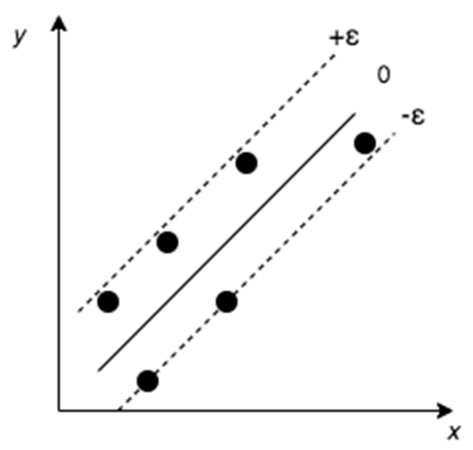
2.2. Support Vector Machines (SVMs)

The SVM, also known as Support Vector Regression (SVR) for numeric prediction, is an algorithm for classification and regression that is well known for its high accuracy, modeling highly complex relationships, and for not over-fitting the evaluations [17]. A two-dimensional SVR example is shown in Figure 5, where the bold line is called the hyper plane; this separates the classes and helps to predict the target value, the boundary lines (dotted lines), which create a margin, and the support vectors that are the data points closest to the boundary [19].

The goal is to fit the error within a certain threshold considering the points that are within the boundary line, so the best-fit line is the hyperplane line that has the maximum number of points.

The hyperplane line is described in Equation (6), where $\beta$ is the coefficient and $\alpha$ is the intercept.

$$Y_{stations}=\beta X+\alpha ,$$

(6)

Equations (7) and (8) denote the boundary lines, and the hyperplane is the one that satisfies Equation (9).

$$\beta X+\alpha =+ϵ,$$

(7)

$$\beta X+\alpha =-ϵ,$$

(8)

$$-ϵ \le Y_{stations}-\beta X-\alpha \le +ϵ,$$

(9)

considering the fact that $Y_{stations}-\beta X-\alpha =0.$

2.3. Artificial Neural Network (ANN)

An ANN algorithm models the relationship between a set of input signals and an output signal using a model derived from the understanding of how a biological brain responds to sensory inputs; the algorithm uses a network of artificial neurons (nodes) to solve learning problems in which there may be classification or numerical prediction problems [17].

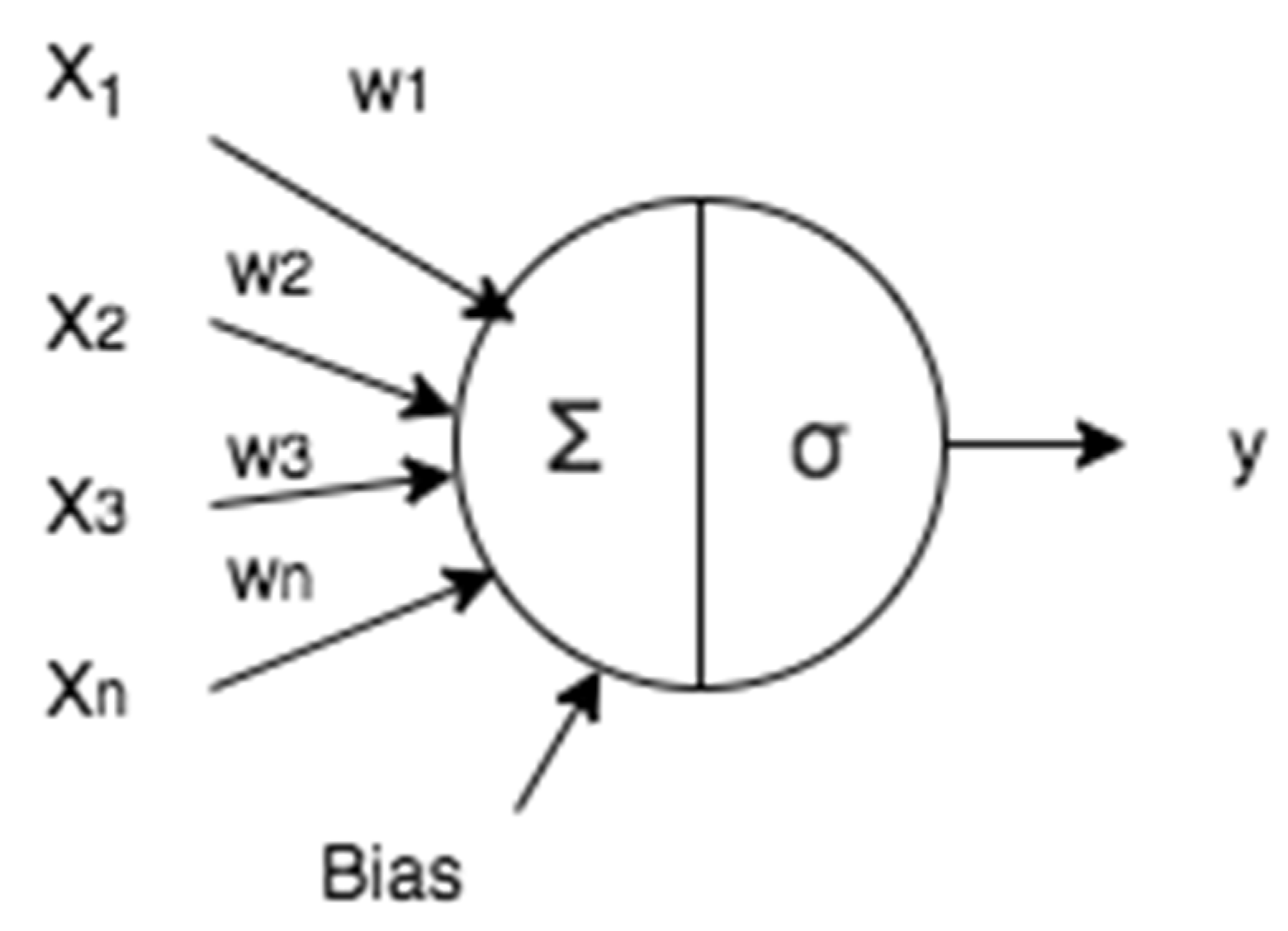
The biological neural networks are composed of dendrites, soma and axon, and the dendrites are responsible for capturing the nerve impulses that emit other neurons. These impulses are processed in the soma and they are transmitted through the axon to contiguous neurons [20]. Following this scheme, an artificial neuron is composed of inputs that in our case are the annual averages of albedo, Linke, cloudiness index and altitude denoted by X₁ to X_n, with a weight for each input denoted by w and a bias. The activation function is how the data will be modeled, so for example in numeric predictions a linear function is perfect for regression and correlation problems, because it uses the linear equation; the output could be an annual daily irradiation measurement. Figure 6 describes an artificial neuron or node.

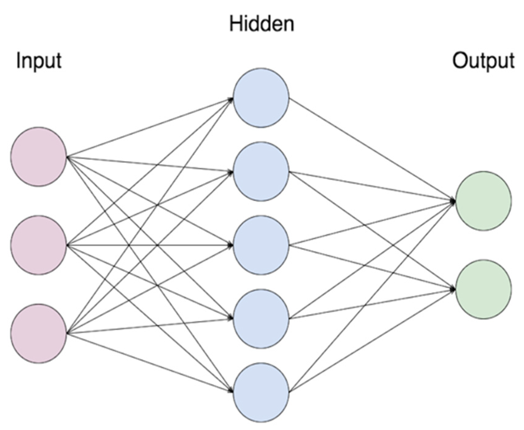
Following the same principles, an ANN is then formed by multiple artificial neurons connected to each other and grouped in different layers, in which the results from an output layer are the input for the next layer. As can be seen in Figure 7, the hidden layers are the layers between the input and output layers.

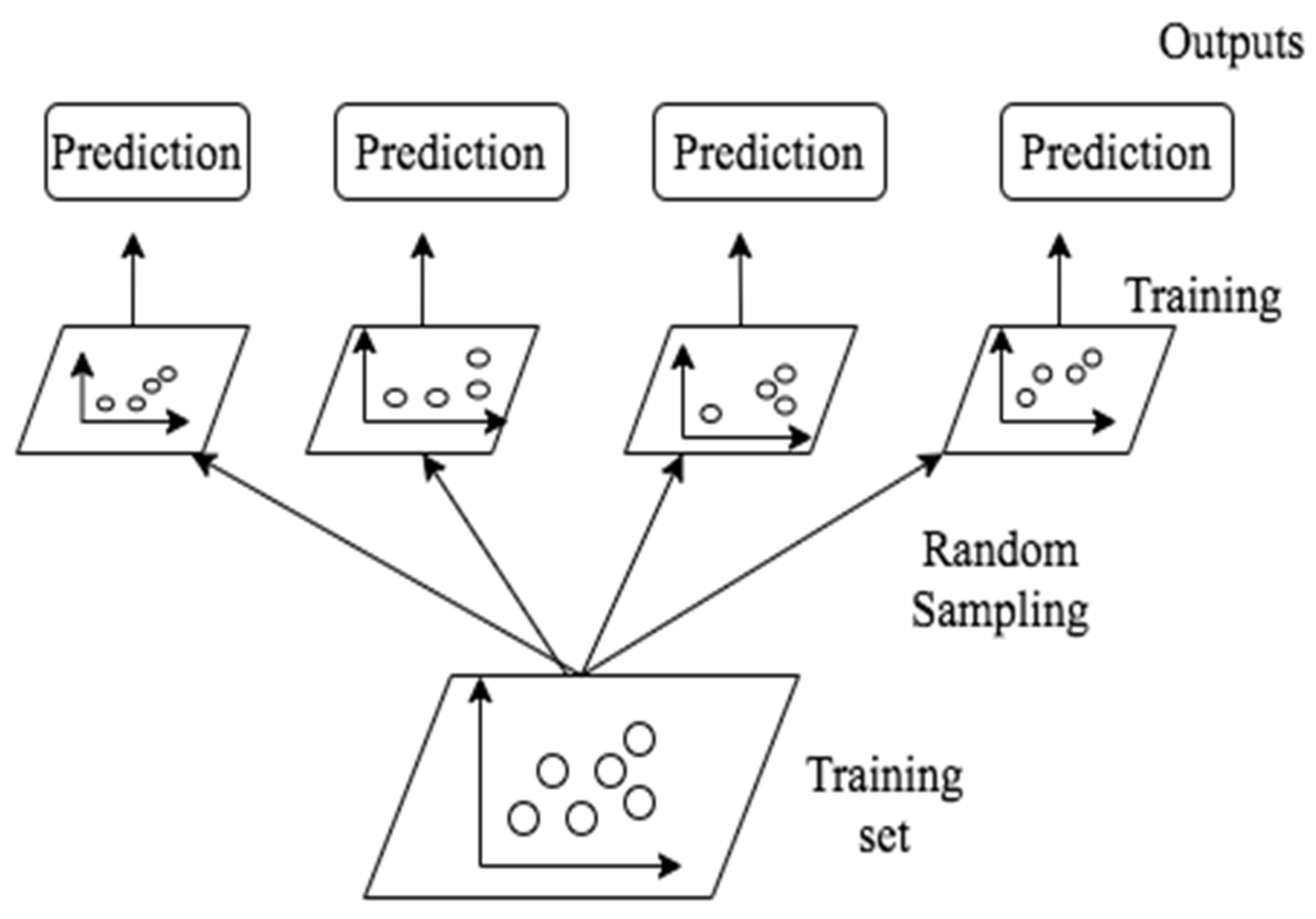
2.4. Random Forest (RF)

RF is a method that combines the predictions from a lot of algorithms with the purpose of obtaining a better result. Random Forest uses an approach called Bagging, and this approach permits that varied instances from a set of data be sampled and evaluated with the same algorithm; the final output is the most frequent value in the predictions [21]. Figure 8 shows the structure of the Random Forest method.

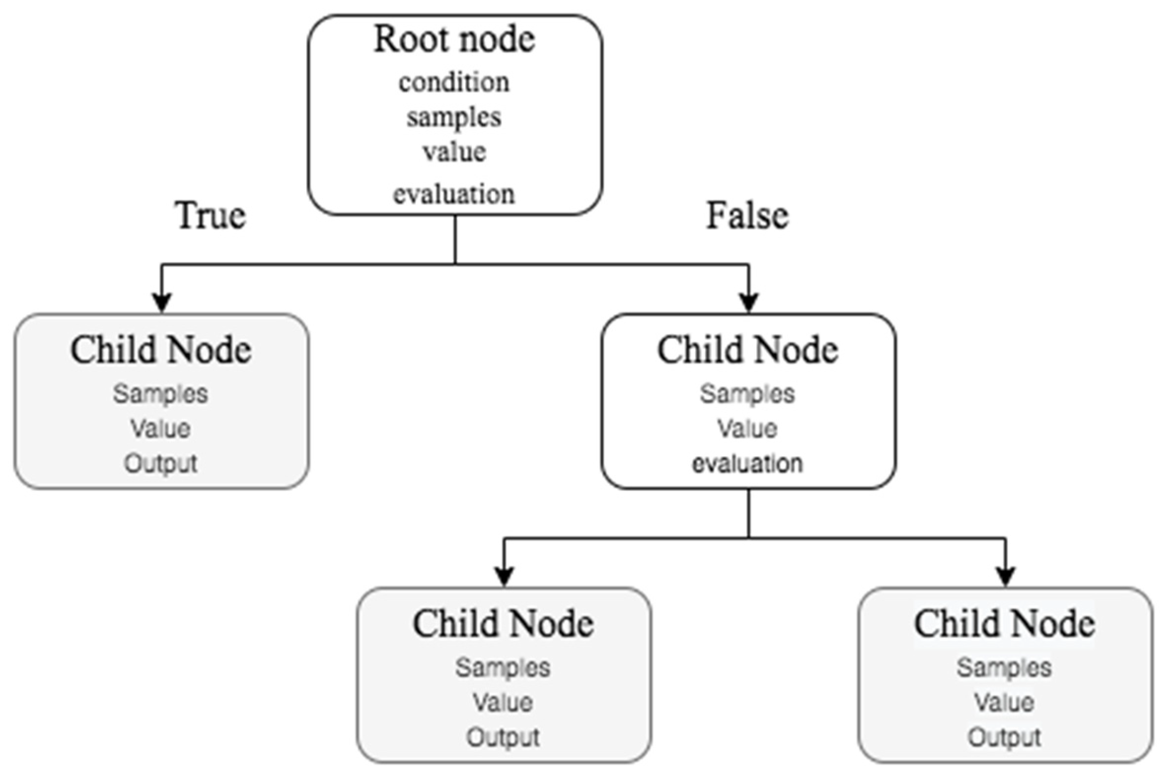
The default algorithm used for RF is the decision tree; this algorithm utilizes a tree structure to model the relationships between the features and the outcomes [21]. It begins with a root node (depth 0) and the algorithms start to make conditions or assumptions about the data; if the assumptions are true, then it moves to the root’s left child node (depth 1, left). In this case, this is a leaf node that does not have any children nodes, so the node predicts the output. If the conditions are false, then it moves to the right child node. Figure 9 shows an example of the decision tree.

The decision tree involves growing the tree. First, it splits the set in two subsets using a single feature k and a threshold t_k, which can be seen as “What value of k is lower or equal to t_k?”. The algorithm searches for the pair (k, t_k) that splits the set in a way that minimizes the Mean Squared Error (MSE), as it is described in Equation (10). The m_left/right is the number of instances in the left and right set and m is the total of instances.

$$J\left(k,t_k\right)=\frac{m_{left}}{m} ms{e}_{left}+\frac{m_{right}}{m} ms{e}_{right }$$

(10)

where $\left\{MS{E}_{node}={{\displaystyle \sum }}_{iϵnode}{({\widehat{y}}_{node}-y^{\left(i\right)})}^2{\widehat{y}}_{node}=\frac{1}{m_{node}}{{\displaystyle \sum }}_{iϵnode}{y}^{\left(i\right)}\right\}$.

As can be seen, the random forest is a set of decision trees which are trained through random samples and the result is the most frequent MSE score in all the trees.

3. Results

In a previous work [1], the L-method was used with clustering algorithms such as GMM and K-means; the results showed that the evaluations with 17 and 10 clusters gave a better model to explain the relations between climate features and the yearly daily irradiation, and the best model was for 17 clusters. In this study, 4 and 17 classes were evaluated with the k-means algorithm, and 10, 8 and 11 classes using the GMM algorithm.

The annual daily irradiation data of the 26 stations are described in

Table 2. Stations with their annual daily irradiation and cluster class; the 4 and 17 classes were clustered by K-means algorithm and the others by GMM algorithm.

Station Number	Annual Daily Irradiation (Wh/m2)	4 Classes	17 Classes	10 Classes	8 Classes	11 Classes
1	4391	2	16	10	2	10
2	4747	2	16	10	2	10
3	4772	4	1	3	8	3
4	4803	3	14	9	4	9
5	4900	4	1	3	8	3
6	5061	2	16	10	2	10
7	5198	1	12	5	1	1
8	5243	4	4	8	3	8
9	5251	4	4	8	3	8
10	5297	4	7	1	6	11
11	5349	4	1	3	8	3
12	5378	4	11	4	5	4
13	5403	4	7	10	2	10
14	5405	2	5	2	2	2
15	5440	1	17	5	5	11
16	5472	4	7	10	8	10
17	5479	1	2	5	1	5
18	5607	2	16	10	2	2
19	5636	4	7	10	8	10
20	5636	2	10	10	2	2
21	5650	1	12	2	1	1
22	5760	1	15	7	7	7
23	5798	4	7	10	2	10
24	5914	2	10	10	2	2
25	5954	1	15	7	7	7
26	5960	1	8	7	7	7

. In addition, the class that belongs to each station is presented.

Table 3. Annual daily irradiation, and annual averages of albedo, Linke, cloudiness sky index and altitude per cluster class.

Evaluation	Cluster	Annual Daily Irradiation (Wh/m2)	Albedo	Linke	Cloudiness Sky Index	Altitude
K-means 4 Classes	3	4803	1.4228	3.9373	0.0724	417
	2	5252	0.9089	3.5908	0.0493	1880
	4	5318	1.0929	4.0504	0.0597	300
	1	5707	1.3156	3.3587	0.0467	1410
K-means 17 Classes	16	4733	0.7651	3.7766	0.0706	2010
	14	4803	1.5362	4.1138	0.0797	279
	1	5007	0.9692	4.1138	0.0768	282
	12	5198	1.1008	3.1486	0.0458	1890
	4	5249	0.9216	4.2178	0.0662	83
	11	5378	1.407	3.8554	0.049	259
	5	5405	0.9852	3.2987	0.0456	2190
	17	5440	0.8627	3.488	0.0515	2050
	2	5479	1.5647	3.6405	0.0448	1340
	7	5521	0.9344	3.9526	0.0435	616
	10	5775	0.9273	3.792	0.039	1450
	15	5857	3.0128	3.4441	0.0413	211
	8	5960	1.7008	2.8913	0.0386	660
GMM 10 Classes	9	4803	1.3981	3.9828	0.0758	412
	3	5007	1.0493	3.1392	0.045	1900
	8	5247	0.9156	4.2207	0.0662	66
	1	5297	0.9402	3.4437	0.0467	1670
	10	5366	0.8934	3.7703	0.0455	1350
	5	5372	1.5972	3.6213	0.0458	1540
	4	5378	1.2612	3.8461	0.0501	590
	2	5405	1.0493	3.1392	0.045	1900
	7	5891	1.9808	3.1757	0.0398	528
GMM 8 Classes	2	4796	0.9246	3.6013	0.0453	1670
	4	4803	1.5312	3.8707	0.0666	666
	8	5226	0.9438	4.0782	0.0631	520
	3	5247	0.9236	4.2185	0.0652	62
	6	5297	0.9425	3.3914	0.0687	617
	5	5409	1.3758	3.2596	0.0492	1230
	1	5442	1.1262	3.2506	0.0454	1870
	7	5891	1.8938	3.2506	0.0405	503
GMM 11 Classes	9	4803	1.3964	3.9956	0.0778	342.9
	3	5007	0.9604	4.1067	0.0694	451.3
	10	5215	0.8762	3.8325	0.0452	1130
	8	5247	0.9162	4.2192	0.0661	65.4
	11	5369	0.8865	3.6482	0.0497	1 430
	4	5378	1.7276	3.8701	0.0481	143.3
	1	5424	1.0966	3.2068	0.0458	1 930
	5	5479	1.7575	3.6715	0.046	1 360
	2	5641	0.9961	3.3851	0.045	2 090
	7	5891	1.8781	3.1055	0.0396	593.3

contains the annual daily irradiation values by class as well as the annual measurements of albedo, Linke, cloudiness index and altitude for each algorithm and k clusters; the data are sorted as the lowest to highest Annual Daily Irradiation value and the classes that are exempt are because in these regions there are no stations to evaluate. The cluster column indicates the region; for example, the index GMM10 in the cluster column has a 3, and this number indicates the region in light blue shown in the map of Figure 2.

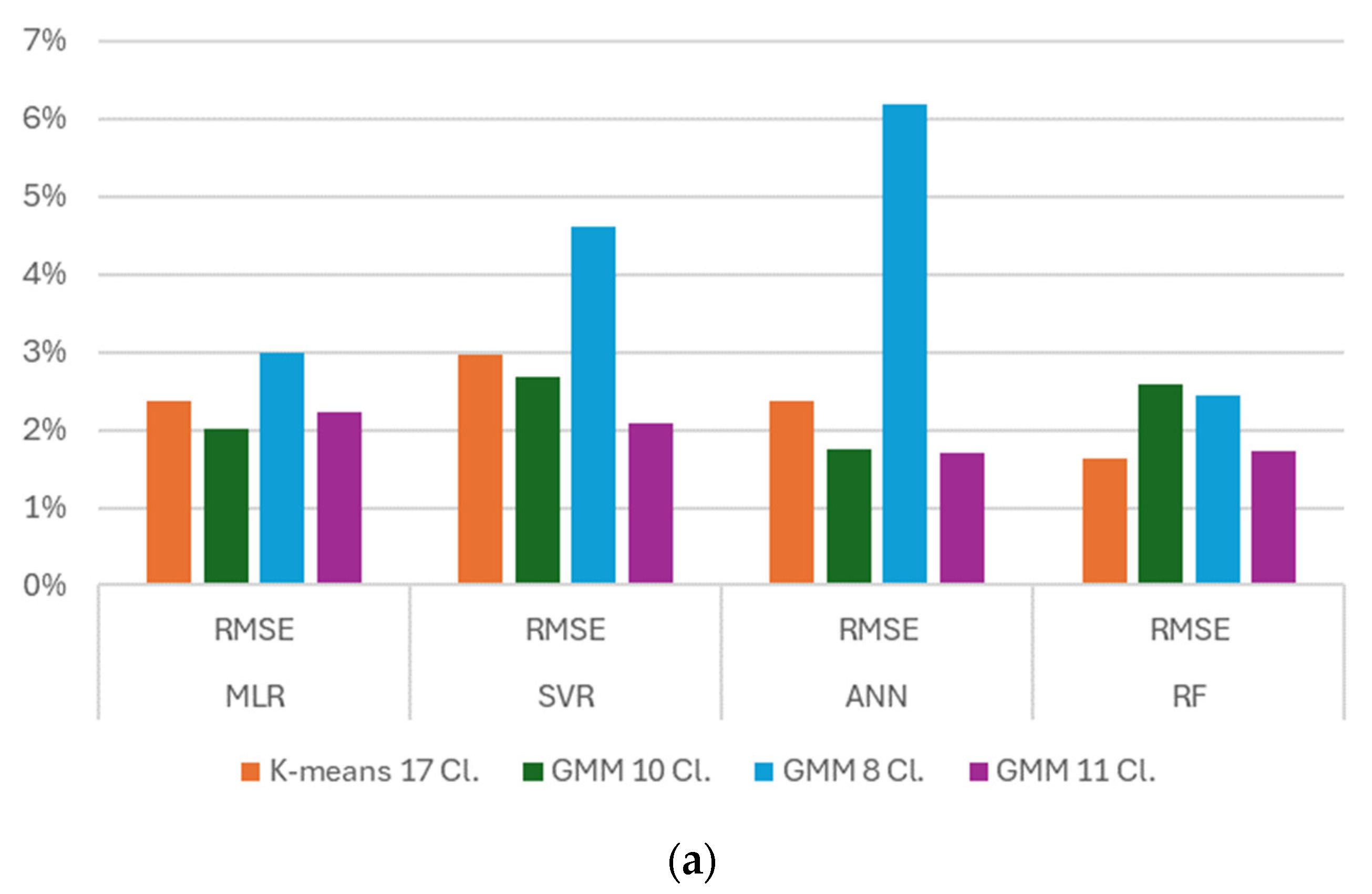
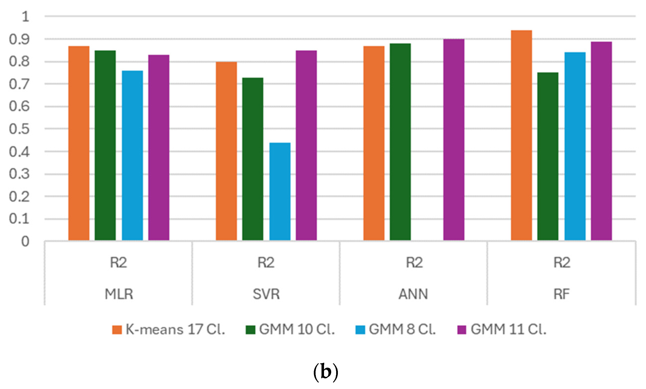
In pursuit of establishing the correlation between Annual Daily Irradiation and climatic features, several machine learning algorithms were employed, and the assessment of their performance relied on the Root Mean Square Error (RMSE) and R-squared (R²) scores. A lower RMSE indicates a more precise regression, suggesting that the model’s predicted values align closely with the actual data. The R² denotes the degree of relationship with the irradiation values.

Table 4. Stations with their annual daily irradiation and cluster class.

Evaluation	Linear Multiple Regression		SVR		ANN		RF
	RMSE	R2	RMSE [%]	R2	RMSE [%]	R2	RMSE [%]	R2
K-means 4 Cl.	0%	1	3.1%	0.80	6.0%	−1	2.8%	0.77
K-means 17 Cl.	2.4%	0.87	3.0%	0.80	2.4%	0.87	1.6%	0.94
GMM 10 Cl.	2.0%	0.85	2.7%	0.73	1.8%	0.88	2.6%	0.75
GMM 8 Cl.	3.0%	0.76	4.6%	0.44	6.2%	−1	2.4%	0.84
GMM 11 Cl.	2.2%	0.83	2.1%	0.85	1.7%	0.90	1.7%	0.89

describes the results for each algorithm.

As can be observed in Table 4 and Figure 10, the k-means algorithm with four classes’ evaluations had the best RMSE and R², but it is more likely that the model is overfitting the scores because of the low quantity of data that can be related in four classes, and that this is why it does not represent a viable relationship with respect to the annual solar irradiation. The better scores were given by ANN and Random Forest algorithm, which were the evaluation with the 17 classes that better described the relationship between the climatic features and the annual solar irradiation. This is good because the optimal number of clusters was given by the L-method, so we can assume that the L-method is a good evaluation technique for obtaining the optimal number of clusters thanks to all the R² scores being greater than or equal to 0.80.

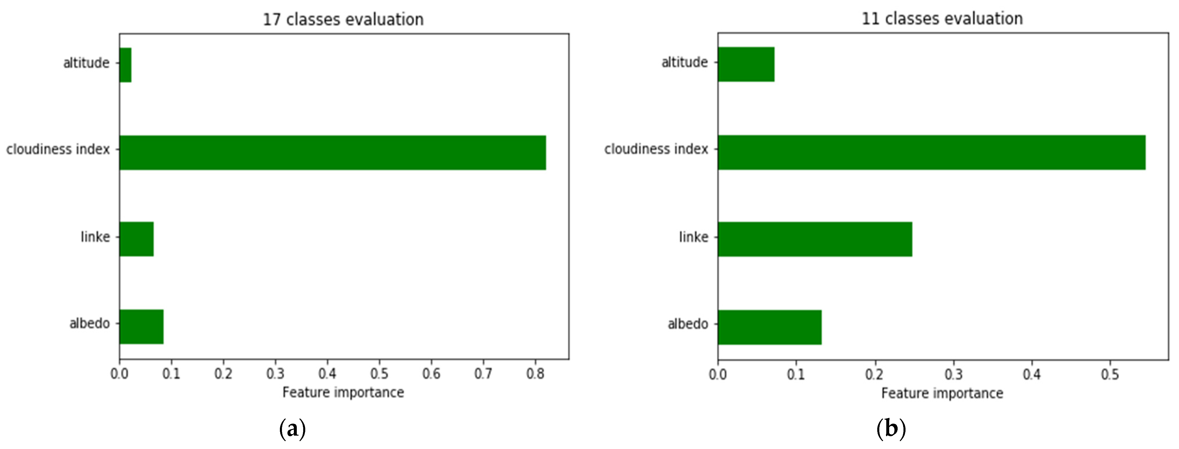
Regarding the importance of the feature, Random Forest offers a way to visualize the relative importance of each feature, as shown in Figure 11.

The cloudiness index is the most important feature, along with the annual solar irradiation, while the remaining features can be considered supportive in the clustering of regions.

In Figure 12, the optimal clustering for Mexico based on Annual Daily Irradiation is illustrated using the k-means algorithm with 17 classes. Despite this being the optimal scenario, notable results are also evident for clustering with 10 and 11 classes. These alternative clustering approaches exhibit favorable indicators for effectively regionalizing Mexico, as evidenced by commendable R² scores.

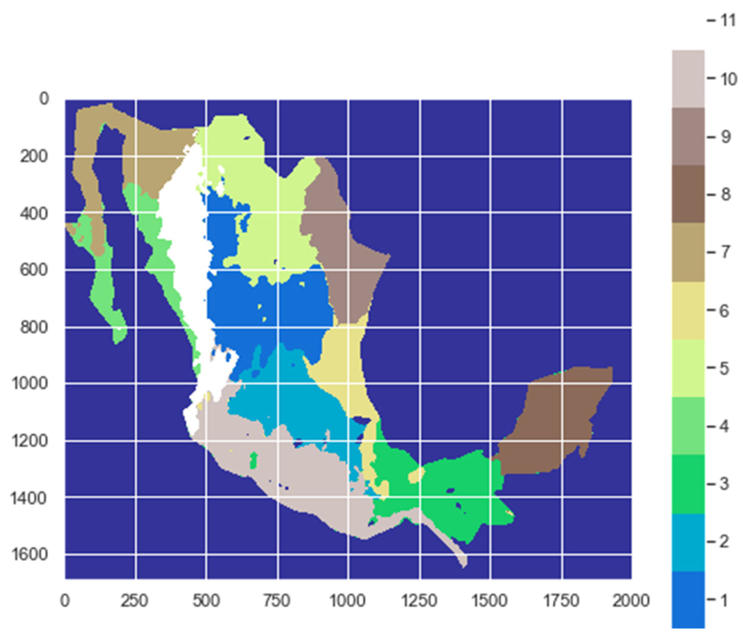
Figure 13 and Figure 14 visually present the regionalization of Mexico under these alternative scenarios, with 10 and 11 classes, respectively. These visual representations emphasize the meaningful subdivisions achieved with a reduced number of classes, reinforcing the effectiveness of the clustering approach for capturing distinctive patterns in solar irradiation across different regions of Mexico. The two figures illustrate the regionalization of Mexico using Gaussian Mixture Models (GMM); it can be seen that the clustering of regions is very similar in both, and they only differ slightly in classes 1 and 2 between the two figures. Upon a closer examination of the data, it was observed that the difference in clustering was attributed to four stations in regions that share similar characteristics and exhibit similar data. It was also observed that by incrementing the number of classes, as shown in Figure 14, the changes in the clustering of regions aligns more closely with the vertical distribution of regionalization with 17 clusters depicted in Figure 12, which was obtained using the k-means clustering technique.

4. Discussion

Solar global radiation data from meteorological stations of the National Weather Service in Mexico were subjected to a comparative analysis with climatic regionalization derived from cluster analysis techniques based on various climatic parameters. The evaluation involved several machine learning algorithms, including Multiple Linear Regression (MLR), Random Forest (RF), Support Vector Machines (SVM), and Artificial Neural Networks (ANN), with the performance metrics of Root Mean Square Error (RMSE) and R² score serving as key outputs.

It is important to consider that the performance of different machine learning algorithms largely depends on the size and structure of the data. The relationships explored in this research are complex due to the nature of the variables and the large amounts of data involved. MLR is particularly useful when modeling relationships that are not overly complex and when information is limited. SVM performs well for complex and nonlinear relationships. RF is an algorithm that seldom exhibits overfitting, and it does not require variable transformation or parameter adjustment. ANNs excel in capturing complex and nonlinear patterns in data, adapting well to prevent overfitting and performing effectively with large datasets.

The results of this comparative analysis revealed that the optimal regionalization was achieved with 17 clusters, employing both ANN and RF algorithms. Notably, RF demonstrated superior performance, exhibiting the best values for both RMSE and R² scores. The aforementioned results align with the advantages associated with both ANN and RF algorithms, taking into account the quantity of data and the complexity of the utilized variables. When fewer classes were considered in the regionalization, it appears that the MLR algorithm exhibited overfitting in the data. Based on the above, the results indicate that increasing the number of classes leads to improved performance across algorithms. Notably, the RF algorithm exhibited no overfitting and appeared to fit the data better in this study, resulting in a more optimal model.

The analysis underscored the significance of the cloudiness index as the primary feature for identifying regions with respect to global solar irradiation. However, Linke turbidity and albedo also proved to be relevant factors in the regionalization process, contributing to a more comprehensive understanding of the climatic factors influencing solar radiation patterns.

The efficacy of the L-method in determining the optimal number of clusters was highlighted, with the results aligning with the best RMSE and R² scores. This emphasizes the practical utility of the L-method in guiding clustering processes related to the delineation of geographic regions based on climatic parameters. Additionally, the comparison of multiple algorithms provided a robust means of evaluating and validating both the data and results, offering insights into the strengths and limitations of different approaches. This comprehensive approach enhances the reliability and validity of the regionalization model, particularly when dealing with climatic variables and solar irradiance data. The findings contribute to advancing the understanding of regional solar resource distribution and offer valuable insights for the optimization of solar energy planning and utilization.