
Estimation of PM2.5 and PM10 Mass Concentrations in Beijing Using Gaofen-1 Data at 100 m Resolution


1
School of Environment and Spatial Informatics, China University of Mining and Technology, Xuzhou 221116, China
2
Artificial Intelligence Research Institute, China University of Mining and Technology, Xuzhou 221116, China
3
School of Computing and Mathematics, College of Science and Engineering, University of Derby, Kedleston Road, Derby DE22 1GB, UK
*
Author to whom correspondence should be addressed.
Remote Sens. 2024, 16(4), 604; https://doi.org/10.3390/rs16040604
Submission received: 17 December 2023
/
Revised: 28 January 2024
/
Accepted: 30 January 2024
/
Published: 6 February 2024
(This article belongs to the Section Atmospheric Remote Sensing)
Abstract
:Due to the advantage of high spatial coverage, using satellite-retrieved aerosol optical depth (AOD) data to estimate PM2.5 and PM10 mass concentrations is a current research priority. Statistical models are the common method of PM estimation currently, which do not require the knowledge of complex chemical and physical interactions. However, the statistical models rely on station data, which results in less accurate PM estimation concentrations in areas where station data are missing. Hence, a new hybrid model, with low dependency on on-site data, was proposed for PM2.5 and PM10 mass concentration estimation. The Gaofen-1 satellite and MODIS data were employed to estimate PM2.5 and PM10 concentrations with 100 m spatial resolution in Beijing, China. Then, the estimated PM2.5/10 mass concentration data in 2020 were employed to conduct a spatio-temporal analysis for the investigation of the particulate matter characteristic in Beijing. The estimation result of PM2.5 was validated by the ground stations with R2 ranging from 0.91 to 0.98 and the root mean square error (RMSE) ranging from 4.51 μg/m3 to 17.04 μg/m3, and that for PM10 was validated by the ground stations with R2 ranging from 0.85 to 0.98 and the RMSE ranging from 6.98 µg/m3 to 29.00 µg/m3. The results showed that the hybrid model has a good performance in PM2.5/10 estimation and can improve the coverage of the results without sacrificing the effectiveness of the model, providing more detailed spatial information for urban-scale studies.

1. Introduction
Numerous health-related studies have shown that exposure to PM2.5 and PM10 increases morbidity and mortality from a number of diseases, most of which are respiratory and cardiovascular diseases [1,2,3,4,5]. There are even adverse effects on the weights and lengths of newborns [6]. In 2010 and 2014, severe PM2.5 pollution caused over 1.2 million and 1.6 million deaths, respectively [7,8]. As the economy and cities grow in China, PM has become one of the most serious pollutants of air pollution and a widespread concern [9,10].
The existing studies using ground-based stations for air quality assessment can provide high-precision results, but the ground-based monitoring methods inevitably face some problems, such as limited spatial coverage and uneven station distribution [11,12,13]. To overcome the above shortcomings, satellite remote sensing techniques are increasingly being studied for estimating PM2.5/10 concentrations due to their high resolution and wide spatial and temporal coverage [14,15,16,17]. The linear regression of aerosol optical depth AOD-PM2.5 is employed to represent the correlation in many previous studies [18,19]. However, several studies have demonstrated that there is a non-linear relationship between AOD and PM2.5 [20,21]. In addition to this, there are several studies based on other methods such as chemical transport simulation and physical correction for PM estimation [22,23,24,25,26]. Among these models, statistical models are the most popular in academia, which include mainly empirical statistical models, such as multiple linear regression [21,27], the mixed effects model [28,29], geographically weighted regression models (GWR) and their derivative models [30,31,32,33], the generalized additivity model (GAM) [34,35,36,37], and machine learning, such as random forest [38,39,40], support vector regression [41,42], and neural network models [43,44,45]. Specifically, the GWR model is a spatial statistical technique used to explore and model spatially varying relationships, which recognizes the variability in connections between variables across geographical locations, enabling focused modeling and analysis. Song et al. applied a specific satellite-based GWR model to obtain PM2.5 over the Pearl River Delta region in China, and developed more accurate large-scale PM2.5 monitoring [46]. The improved geographically and temporally weighted regression (IGTWR) model is developed based on the traditional GWR model, which incorporates both spatial and temporal dimensions to improve the accuracy of predictions. He and Huang employed the IGTWR model for estimating high-resolution PM2.5 over the Beijing–Tianjin–Hebei region of China [47]. By combining temporal and spatial weights, the IGTWR model can consider the geographical and temporal variations of PM2.5 concentrations. This approach recognizes the temporal fluctuations in air quality and provides a more comprehensive and accurate representation of the factors influencing PM2.5 levels over time.
Urban structures are closely correlated with air pollution [48]. To further understand the mechanisms of the models, validate modeling results, and improve modeling capabilities, the particulate matter estimation for urban agglomerations requires high spatial and temporal resolution observations [49]. The Gaofen-1 (GF-1) satellite is a high-resolution Earth observation satellite developed by China. GF-1, launched on 26 April 2013, is part of China’s high-resolution Earth observation system (Hi-ResEOS), and also represents a significant milestone in China for enhancing satellite remote sensing capabilities. It can improve its role in Earth observation with several key features and capabilities it possesses. With advanced optical instruments, it can offer more detailed observations of Earth’s surface features. Additionally, its wide swath coverage can efficiently monitor large areas in a single pass and contribute to comprehensive Earth monitoring. Moreover, GF-1 supports versatile imaging modes, including panchromatic and multispectral, enabling a range of applications in environmental monitoring, pollution assessment, and various applications related to Earth observation. These features collectively make GF-1 a valuable asset for diverse remote sensing endeavors. Several studies have been conducted to retrieve AOD at 160 m spatial resolution and calculate PM2.5 using the Gaofen-1 satellite [50,51]. Furthermore, the AOD data from the moderate resolution imaging spectroradiometer (MODIS) satellite have a high temporal resolution, global coverage, diverse spectral bands, specialized algorithms, rigorous validation, and long-term record advantages. In our previous study, GF-1 wide field-of-view (WFV) and MODIS data were applied to retrieve AODs at a spatial resolution of 100 m [52]. Then, these AODs were employed to estimate PM2.5 and PM10 concentrations at this resolution using an IGTWR model incorporating a proportional relationship formula. The spatial pattern and accuracy of GF PM2.5/10 estimates were assessed using tenfold cross-validation, leave-one-out validation, and validation based on in situ monitoring data. Finally, the limitations of GF PM2.5/10 in this study are discussed, and future work is proposed to address the limitations in resolution and accuracy.
2. Study Area and Data
2.1. Study Region
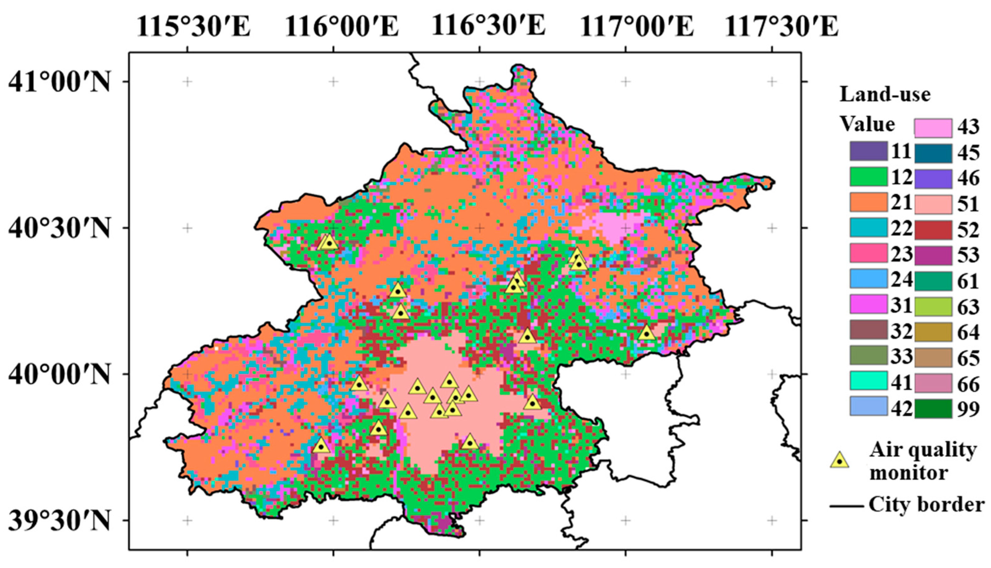
The primary area of focus in this study is Beijing, centered at longitude 116°20′ East and latitude 39°56′ North, a world-famous ancient capital and modern international city. As illustrated in Figure 1, Beijing has 23 types of land use and 24 air quality stations. Due to industrialization and urbanization in recent years, air pollution, especially PM2.5 and PM10, has become a serious and urgent issue for Beijing [11,53,54].
2.2. PM2.5/10 Measurement Data
The PM2.5/10 ground-based measurement data employed in the present paper are collected from the Chinese National Real-Time Air Quality Release Platform (https://air.cnemc.cn:18007/, accessed on 2 December 2023). Figure 1 shows the geographical locations of the national air quality monitoring stations within the Beijing region in 2020. The monitoring stations measure air pollutant parameters including PM2.5, PM10, and ozone. In this study, PM2.5/PM10 at 10:00 and 14:00 are adopted to correspond to the AOD data. In the section on results validation, monitoring data from 40 stations in and around the Beijing city area were used.
2.3. AOD Data
GF-1 combines high resolution with large bandwidth, and accommodates multiple spatial resolutions, multiple spectral resolutions, and integrated multi-source remote sensing data requirements. It has 16 m spatial resolution and four days’ temporal resolution [56]. MODIS is a medium-resolution imaging spectrometer that carries two satellites, Terra and Aqua. It is a crucial instrument in the U.S. Earth Observing System (EOS) program and is primarily used to observe global biological and physical processes. Numerous research fields already make extensive use of the MODIS sensors on Terra and Aqua. They can offer up to two observations of visible light each day. In order to further improve the spatial resolution of the AOD data and to enhance the ability to study air pollution in small areas, Bai et al. combined two sets of satellite data to obtain a high-resolution AOD [52]. First, they collected 52 high-coverage images from the GF-1 wide field-of-view (WFV) cameras within the study area in 2020, along with corresponding MODIS data captured during the same period. The 1 km resolution 1B level data (MOD/MYD02) from MODIS were downscaled with the help of GF-1 WFV data using the mutual information (MI) algorithm [52]. In this process, MI quantifies the statistical dependence between two variables by measuring the amount of information one variable provides about the other, and computes the entropy of each variable and their joint entropy for capturing the uncertainty and information shared between them [57,58]. Then, the downscaled TERRA and AQUA satellite data are used to retrieve AOD by the synergetic retrieval of aerosol properties algorithm (SRAP) [59,60]. Finally, high spatial resolution AOD data of the Beijing area with 100 m spatial resolution are obtained [52]. The AOD data used in this study are those calculated in our previous study, and the validated correlation coefficient is approximately 0.88 in Beijing, which shows promising relationships [52].
2.4. Meteorological Data
Boundary layer height (BLH) data were provided through the ERA-5 from the European Centre for Medium-Range Weather Forecasts (http://www.ecmwf.int/, accessed on 4 December 2023). The meteorological data used in this study were provided in the database at a spatial resolution of 0.25° × 0.25°. The temporal resolution has various options, and to correspond to the hourly sampling frequency of PM2.5/10, the temporal resolution of the products selected in this study was hourly. To correspond to the sampling times for PM2.5 and PM10, BLH values were obtained at 10:00 and 14:00 from the previous day.
Relative humidity (RH) data were obtained from the China regional multi-source fusion live analysis at 1 km resolution product (ART_1 km, ground). The 1 km-resolution product of China’s regional multi-source fusion real-time analysis was developed by using ground station observations, satellites, numerical models, and other data, and includes four elements, such as hourly 2 m humidity. The product was provided by the China National Meteorological Operational Intranet (http://data.cma.cn/weatherGis/web/weather/weatherFcst/index, accessed on 4 December 2023).
2.5. Land-Use Variables
PM2.5/10 concentrations are influenced by the subsurface of the land. Land-use data for Beijing in 2020 were collected from the Resource and Environment Data Cloud Platform (http://www.resdc.cn/, accessed on 4 December 2023). The data have a temporal resolution of years and are raster data with a spatial resolution of 1 km generated based on the 2015 land-use remote sensing monitoring data with Landsat TM imagery. The data include 6 primary types of land use (arable land, forest land, residential land, unused land, grassland, water) and 25 secondary types. The legend codes and their corresponding land-use types are listed in Table 1. Compared to China, Beijing lacks three land-use types: permanent glaciers and snow, Gobi, and others.
2.6. Simulation Data Fields
AOD and PM2.5/10 simulation data were obtained from the CAMS (ECMWF Atmospheric Composition Reanalysis 4) global reanalysis (https://ads.atmosphere.copernicus.eu/, accessed on 7 December 2023). The PM2.5, PM10, and AOD data used in the present study have a horizontal resolution of 0.75° × 0.75° at 3 h temporal resolutions. Data were collected at 00:00, 03:00, 06:00, 09:00, 12:00, 15:00, 18:00, and 21:00 local time and then the 10:00 and 14:00 values were obtained by linear interpolation to make them correspond to the sampling times for PM2.5 and PM10. To begin with, the interval in which the unknown points are located was determined based on the eight known data points. Afterward, the weights were calculated using the distance between the unknown and known points. Assuming there is a linear relationship between the data points, the linear model was established based on the known values and the obtained weights. Two unknown moments as independent variables were substituted into the above linear model to calculate the estimations of the required moments.
2.7. Data Integration
In the present study, parameters from different categories were data integrated to ensure the spatial consistency of the data before being incorporated into the model. Meteorological data were resampled to 100 m spatial resolution using bilinear interpolation to obtain the same spatial and temporal resolution as AOD. Simultaneously, the land-use data were reprojected and resampled, and then stored as raster data in tiff format so that they had the same projection and spatial resolution as the AOD data. Furthermore, the AOD and PM data from CAMS were interpolated to have the same temporal resolution as the GF-1 AOD, allowing them to be used as input data in the proportional relationship formula method. Because the data in the large grid center was sampled as point data, the spatial interpolation was not performed on the CAMS data. Thereafter, the geographic location of the PM concentrations calculated by the proportional relationship formula method was assumed to be the center of each raster cell and then entered as supplemental site data. Finally, a grid with a spatial resolution of 100 m based on the AOD grid was created to integrate all PM data into records for the model.
3. Methods
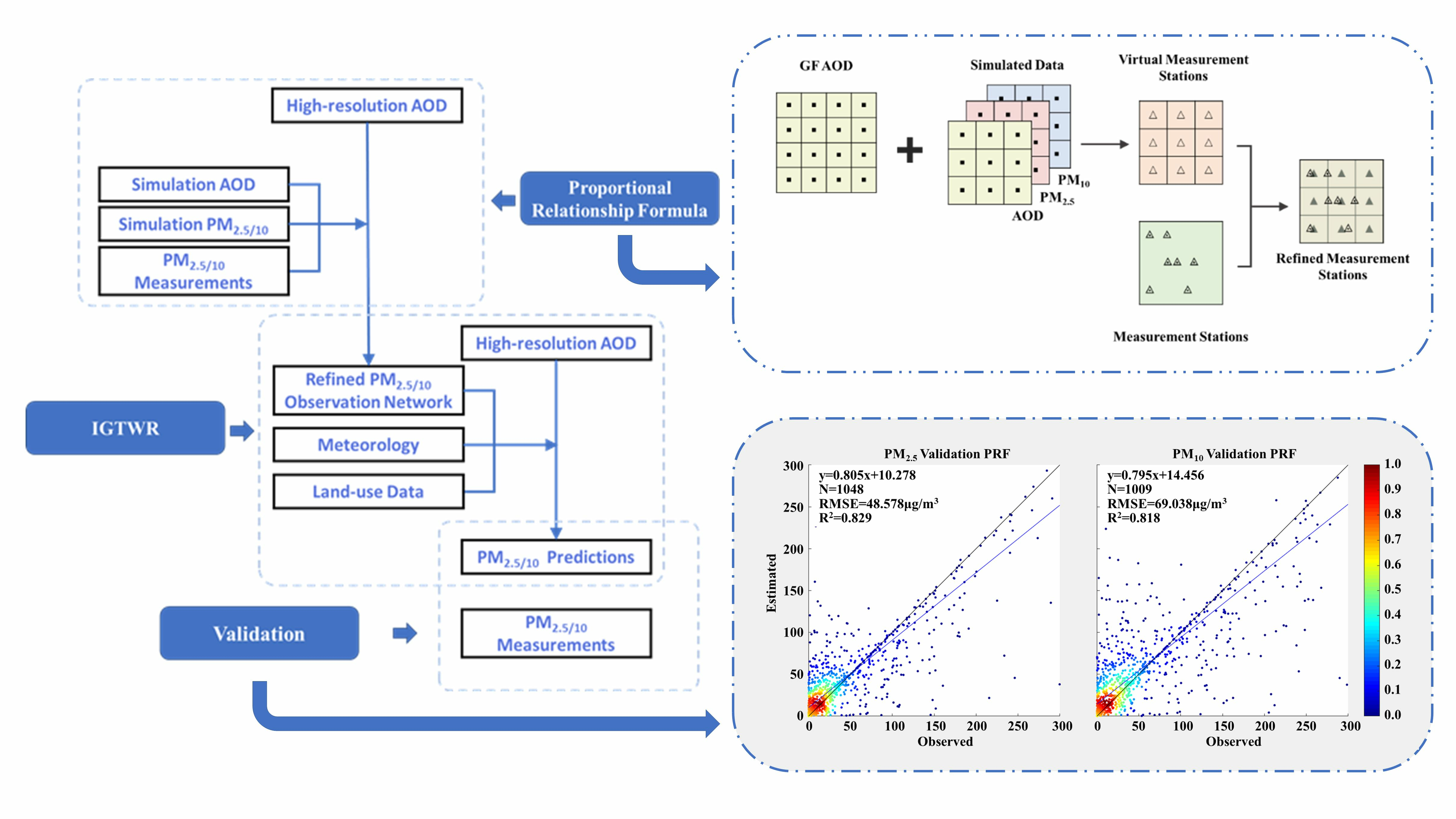
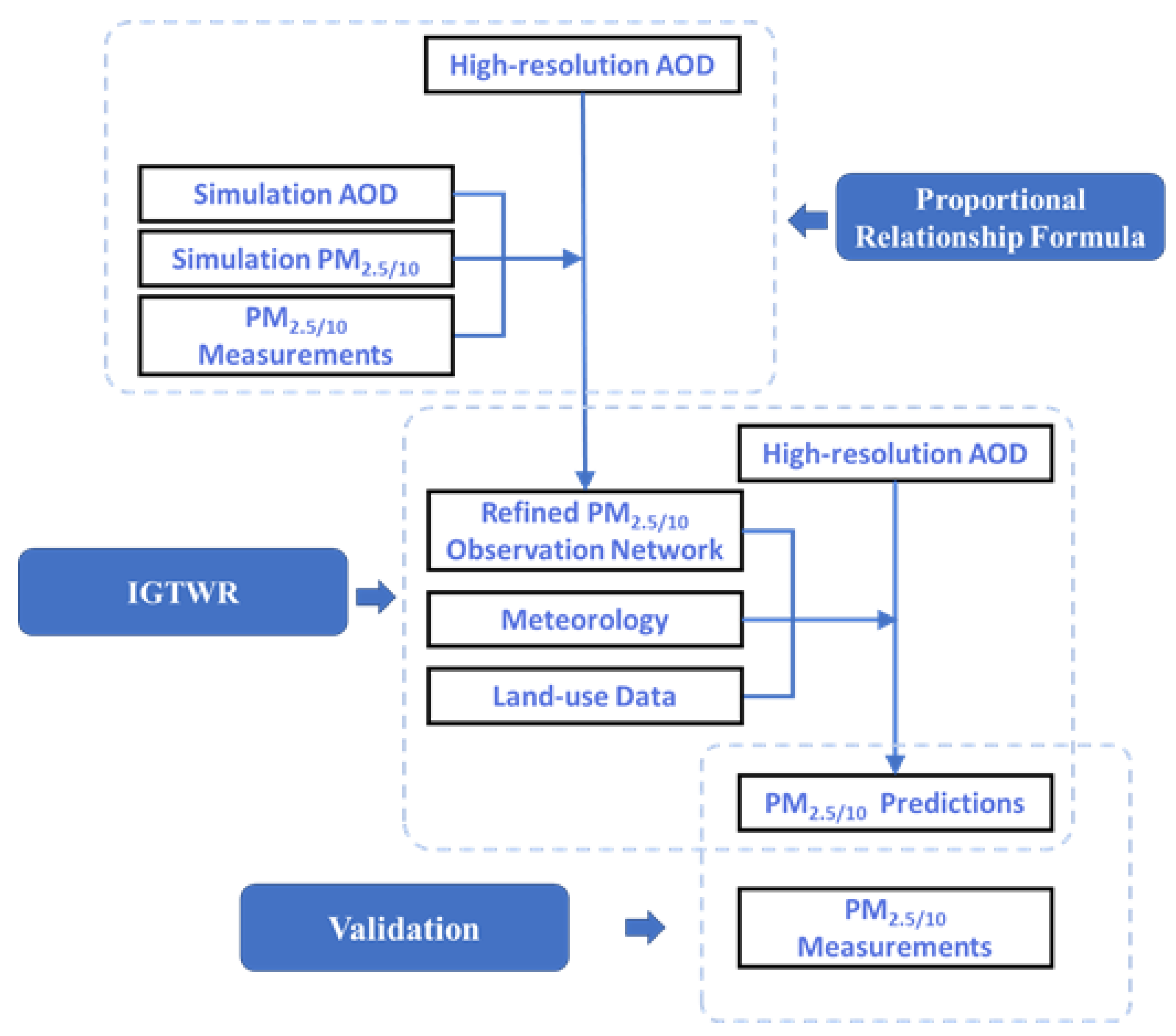
The workflow of the present study is shown in Figure 2. Firstly, a proportional relationship formula was built to establish the refined PM2.5/10 observation network combined with PM2.5/10 measurements (Figure 3). Secondly, an IGTWR model that considers the main parameters, including the AOD, RH, and BLH, was developed to estimate ground PM2.5 and PM10 concentrations [61]. The general distance was defined by latitude, longitude, and land-use classification data. The GTWR model had an encouraging performance with uniform and densely distributed input site observation data [62]. In the developed model, the site-measured PM data were replaced by the refined PM observation network. Finally, cross-validation and ground station validation were used to validate the model performance.
3.1. Proportional Relationship Formula
Due to the vertical distribution and propagation properties possessed by AOD, a method for estimating PM2.5 based on chemical transport models with AOD was proposed. The scaling factor was obtained from the AOD obtained from satellite remote sensing and the model-simulated AOD, and the actual PM2.5 mass concentration was calculated using the scaling factor and the simulated PM2.5 mass concentration [63]. In the present study, the scaling relationship equation was constructed as follows:
The PM2.5 or PM10 concentrations derived from this simple model were referred to as GF PRF PM2.5/10 concentrations in the present study. The terms of particle mass concentrations employed in this analysis are summarized in Table 2.
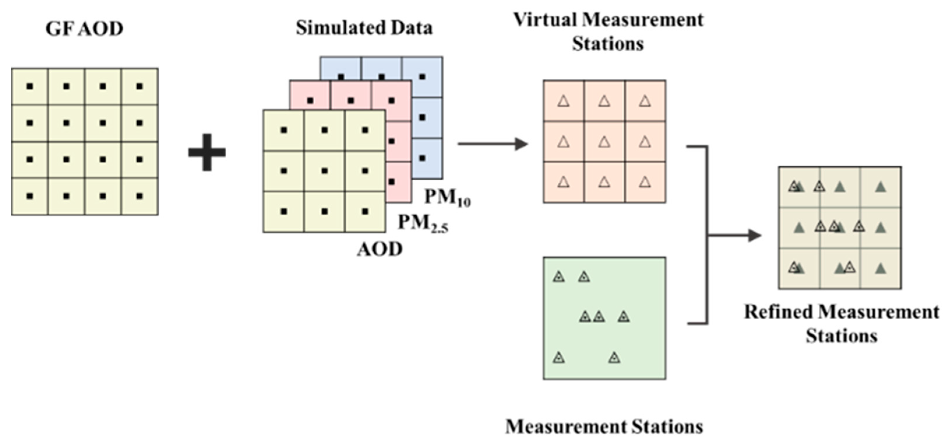
The study area was divided into a standard raster based on simulated AOD data resolution. The centroid position of each raster is used as the latitude and longitude of the fictitious station, and the simulation data are assigned to it.
3.2. IGTWR
Geographic data are affected not only by geographic location but also by time. Given this, a geographically time-weighted regression model was proposed [64]. Xue et al. [61] improved the GTWR model by redefining the generalized distance using land-use data, and the model obtained better performance. In the present study, the IGTWR model was used to estimate the mass concentrations of PM2.5 and PM10 in the study area. The model is shown in (2):
where u0 and v0 denote the longitude and latitude data, d0 and h0 denote the day and hour data, l0 denotes land-use data, and d represents the number of independent variables. In this model, the independent variables are AOD, relative humidity, and boundary layer height; therefore, d is equal to 3 in this equation. i denotes the count of observation points in the refined observation network; yi represents the estimated PM2.5 or PM10 mass concentration. The EVI (enhanced vegetation index) can reflect the extent of capturing particulate matter on plant leaves [65], and NDVI can also be considered in the IGTWR model [66]. Because the study was conducted during the summer months, EVI and NDVI were not considered in the final model. The same fixed bandwidth is used in the present study.
4. Results and Validation
4.1. Results of the Model Fitting and Validation
A virtual monitoring network was established based on the proportional relationship formula in Beijing. PM2.5 and PM10 were estimated using the refined PM2.5/10 measurement network with GF AOD data.
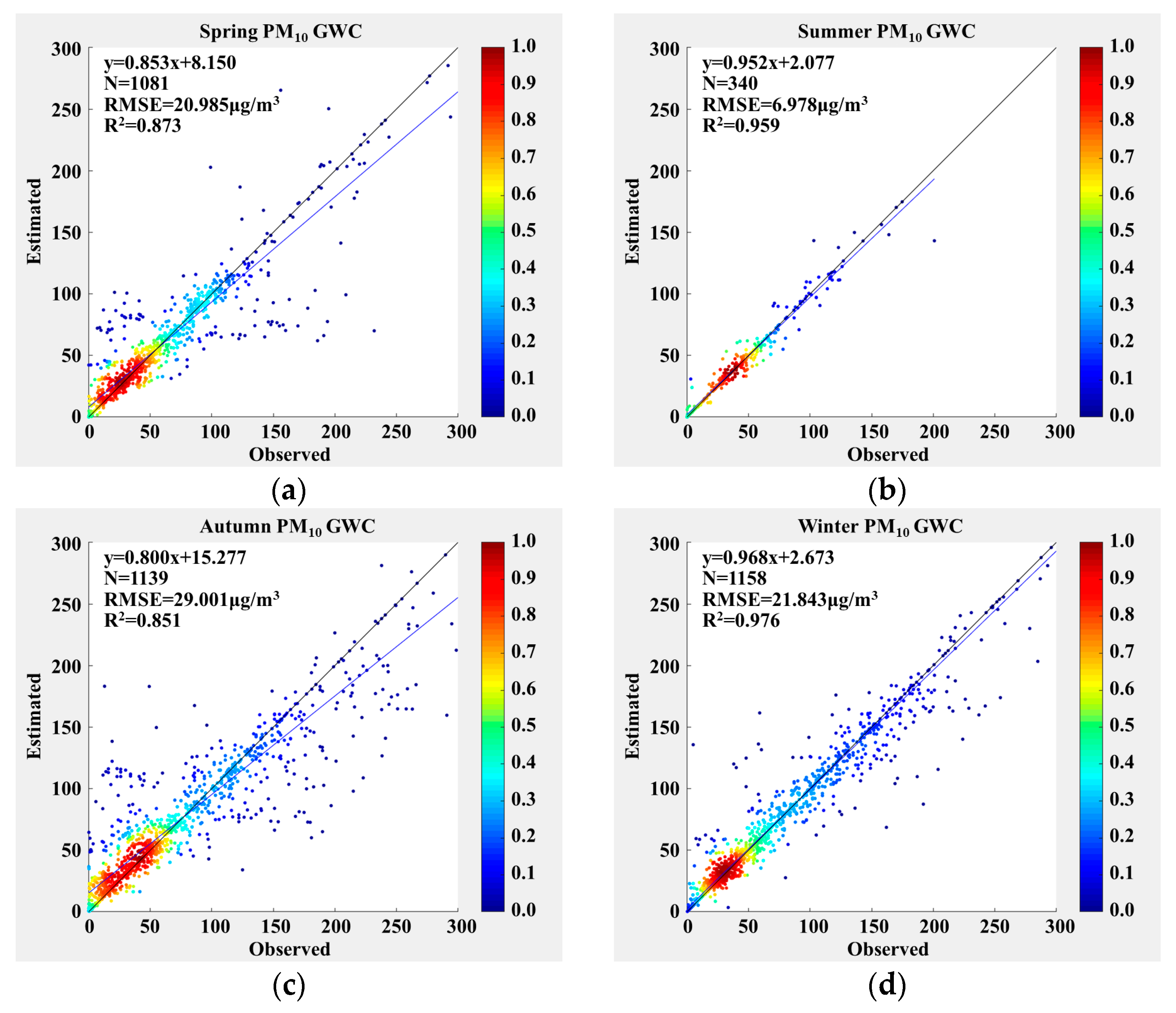
Table 3 shows the coefficient (R2), RMSE, and the coverage of the results for the different methods. The hybrid method of IGTWR and the chemical transport model-based proportional relationship formula was called GWC in this paper. A 1-year dataset was available for modeling in Beijing to obtain as much coverage as possible. In Beijing, PM2.5/10 is positively proportional to AOD, due to PM2.5/10 playing a major role in atmospheric extinction [67]. Higher planetary boundary layer height (PBLH) expands the near-surface atmosphere and promotes vertical convection [68], which means PBLH has a negative correlation with PM2.5/10 mass concentration. As the PM2.5/10 concentration measurement represents dry particles [21], higher air humidity leads to an increase in the value of AOD for the same PM2.5/10 value [24]. Drying the sampling air stream at ground stations eliminates the influence of moisture on particulate mass concentrations when measuring particulate concentrations. Since it is obvious that atmospheric humidity also has a considerable impact on airborne contaminants, relative humidity is also included in the model’s independent variables. That is, RH has a negative correlation with ground-level PM2.5/10.
A linear regression is performed to fit the PM2.5/10 estimation to the monitored PM2.5/10 concentration. Table 3 shows the R2 and coverage of the improved and original models in this paper. These results indicated that PM2.5/10 estimated by the hybrid model combined with GF AOD is in good agreement with PM2.5 measurements on the ground. Moreover, with the inclusion of the “virtual site” data, the GWC model allows for the calculation of PM2.5/10 concentrations using AOD data that do not cover the ground monitoring stations. Therefore, the hybrid model significantly improves the coverage of valid results.
4.2. PM Estimation Using Satellite Remotely Sensed Data
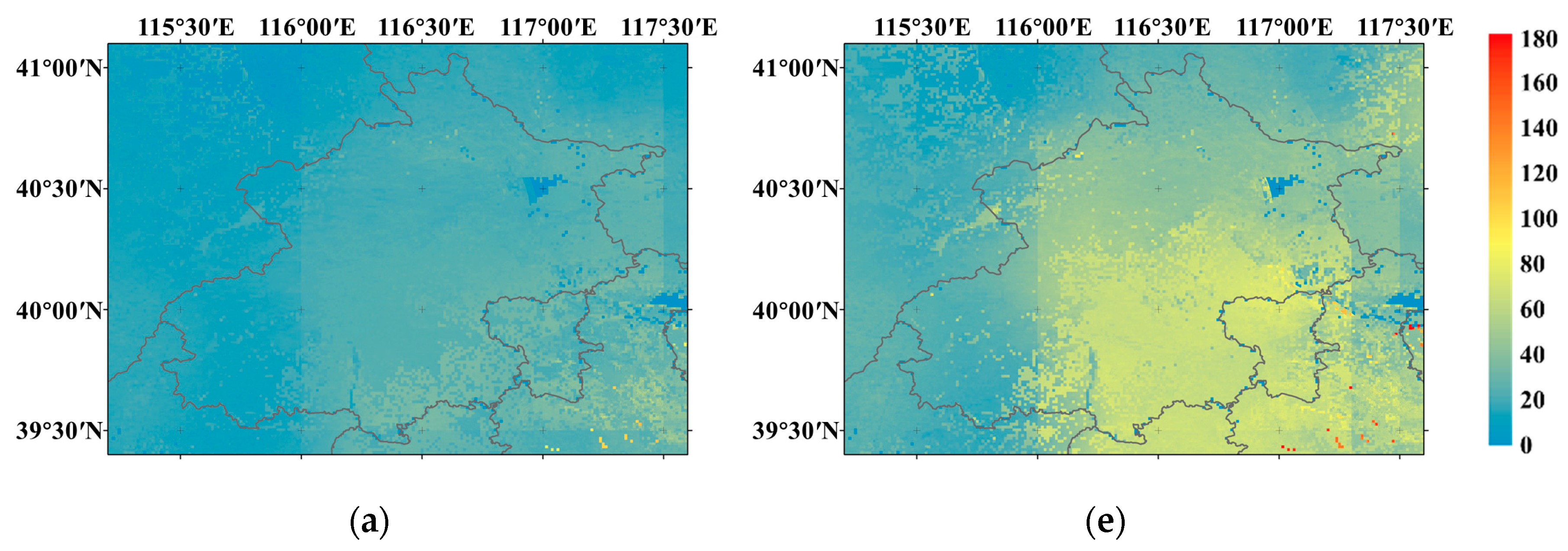
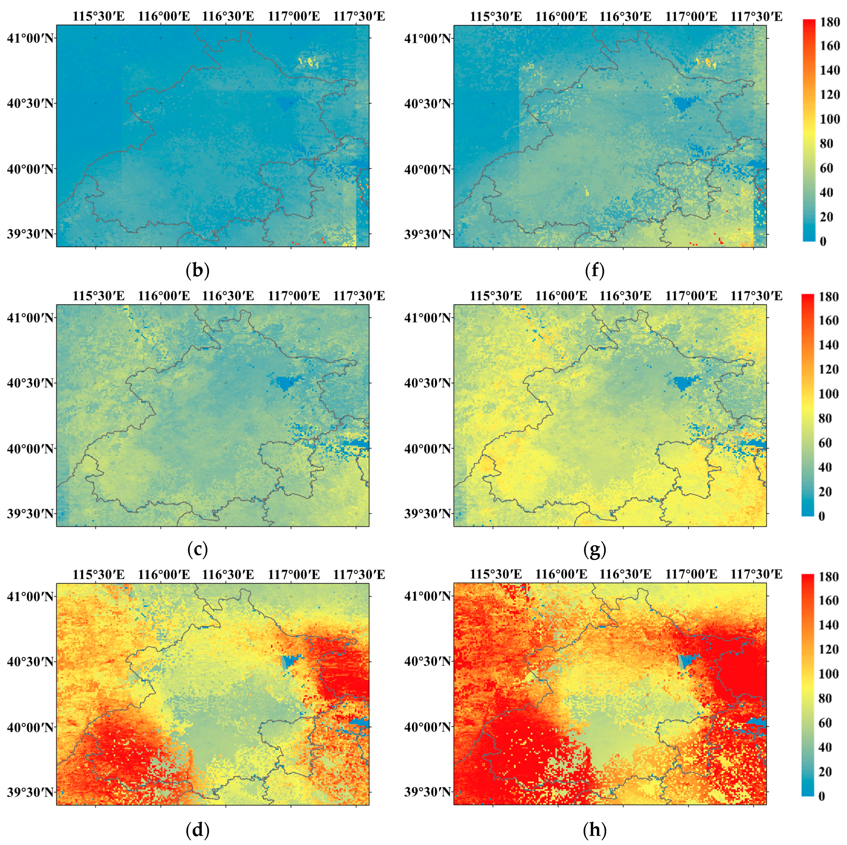
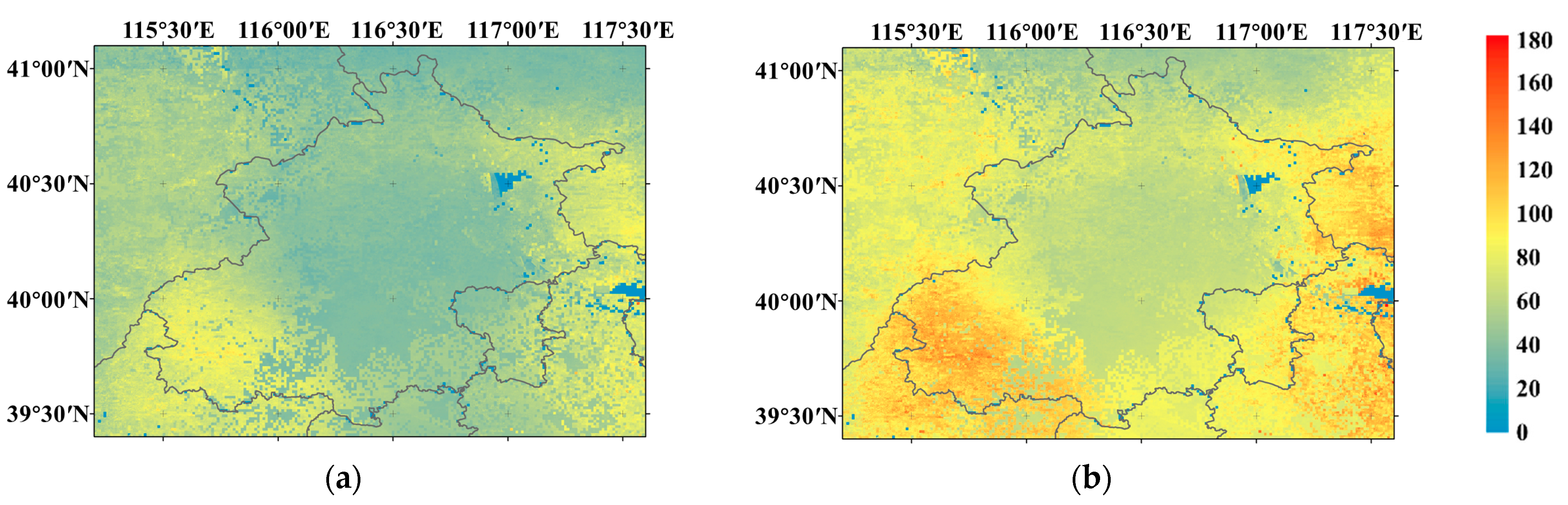
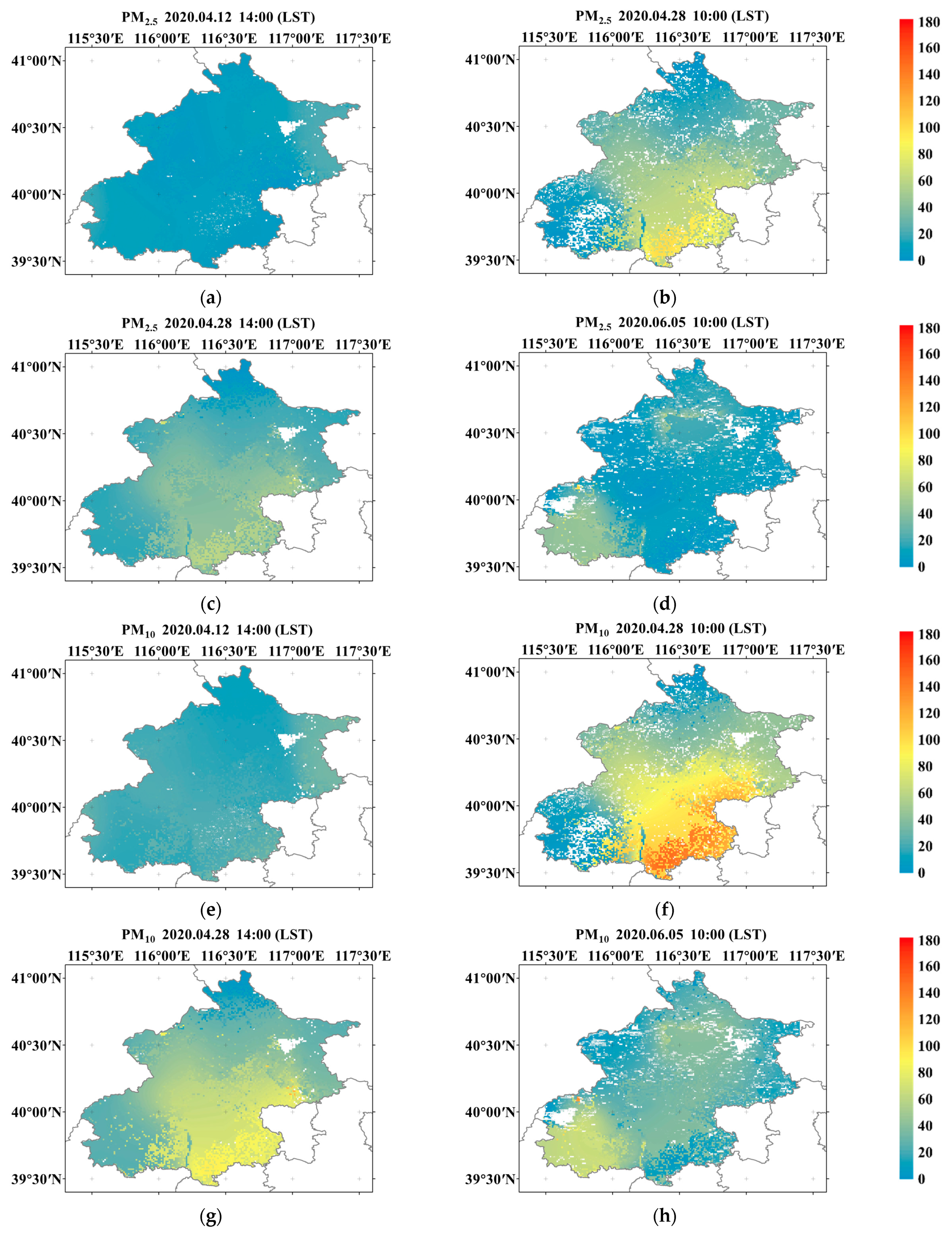
Figure 4 shows the seasonal PM2.5/10 concentrations at a 100 m resolution. Figure 5 shows the annual mean PM2.5/10 concentrations estimated by the IGTWR model at a 100 m resolution in 2020, respectively. Figure 6 shows PM2.5/10 concentrations estimated by the IGTWR model at a resolution of 100 m for days with light pollution, heavy pollution, and pollution with prominent spatial characteristics. The polluted weather of PM2.5 and PM10 in Beijing is mainly concentrated in winter, while spring and summer are mostly clean. In contrast, the distribution of PM values in the central and eastern urban areas is relatively stable, and the seasonal characteristics are relatively insignificant. Estimates of PM2.5/10 in the eastern fringe were missing due to insufficient matching of the GF data. The results show that the spatial variation in the mass concentration of PM2.5 is weaker in Beijing during the study time of this study, while the spatial variation in the mass concentration of PM10 is stronger. Particulate matter pollution is more severe in the urban and southeastern suburbs of southern Beijing, where the land has lower vegetation cover and higher population cover. The south-central part of the Beijing region is urban land, and this small area has lower and more stable PM2.5 and PM10 concentrations compared to its neighboring regions. Relatively lighter pollution is found in the mountainous areas of northern and western Beijing, where estimated PM10 concentrations are typically below 40 μg/m3. Highly polluted areas correspond to areas with poor vegetation cover and large populations. Conversely, clean areas are routinely characterized by thick vegetation, poor populations, and high altitudes. As industrial emissions and population density gradually increase from northwest to southeast in Beijing, PM10 also rises along the geographical gradient.
In addition, pollution in the study area is also influenced by pollutants from outside the region. For example, the southern suburbs are affected by pollution from polluted Hebei Province, south of Beijing [69]. In addition, previous studies have shown that the spatial characteristics of particulate matter in the Beijing area are similar to this study [51,69,70]. However, most of the PM2.5/10 estimations are lower than the observations. This is primarily attributable to the fact that most air quality monitoring stations are located in the center of cities or counties with high pollution levels, while most data in remote mountainous areas are reflected in the estimation results with sparse pollution [69]. In addition, in the study area with large water coverage (such as Miyun Reservoir located northeast of Beijing), the calculated results of PM2.5 and PM10 concentration levels are missing or low, which is the reason for the sudden change in data.
5. Discussion
5.1. Effects of the Refined PM2.5/10 Measurement Stations
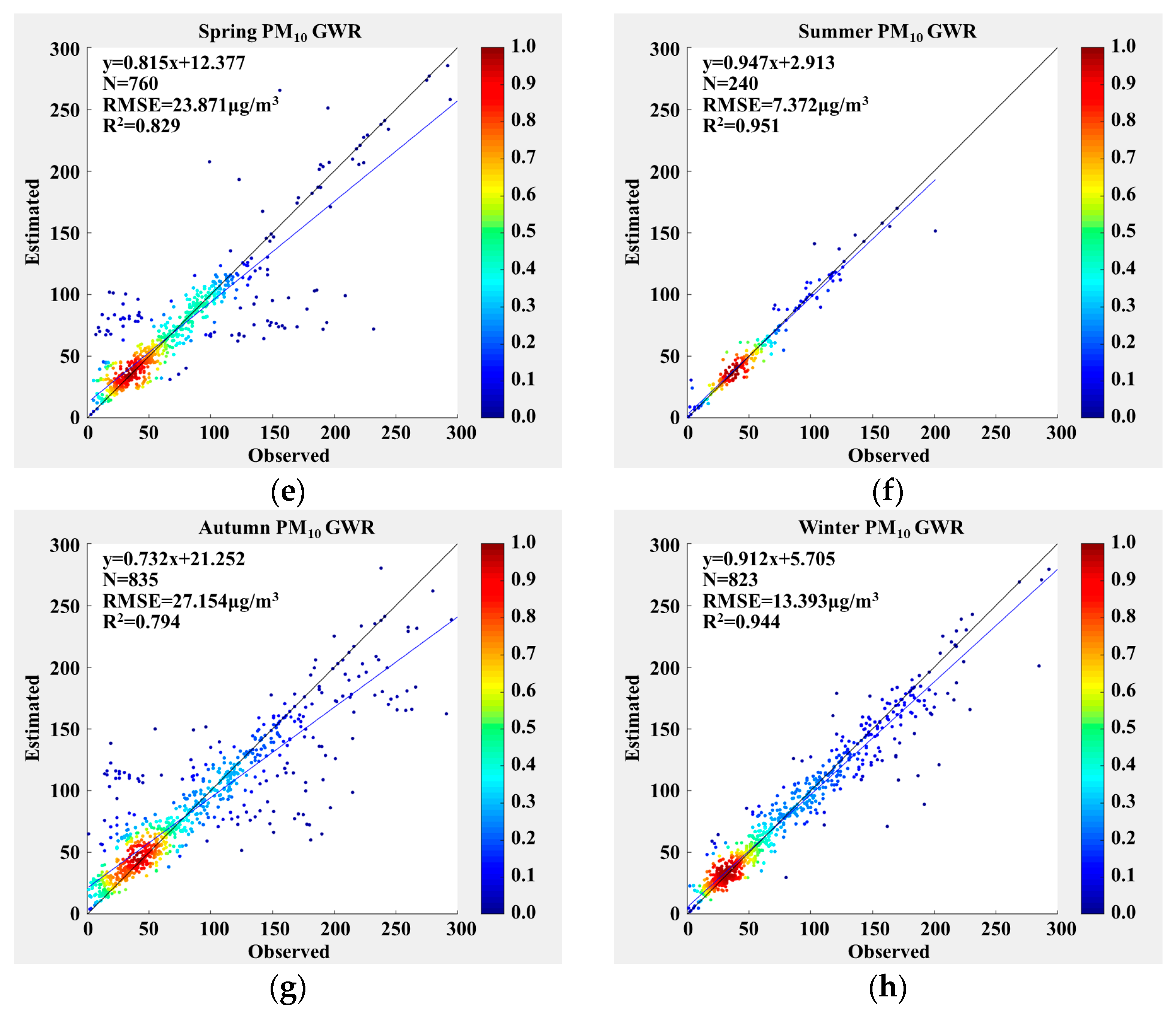
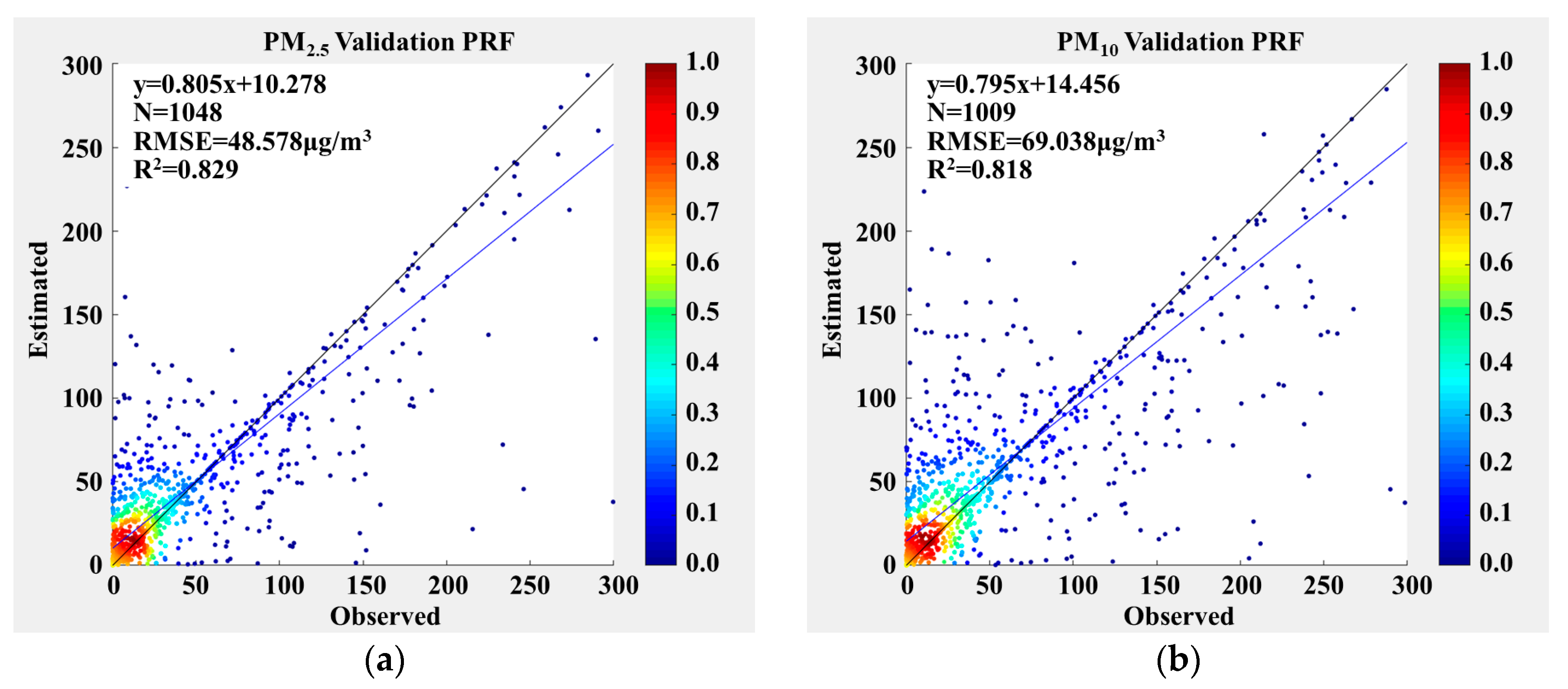
Three experiments were conducted to compare the performance impact of the measurement network before and after refining the model. The first way is to use the proportional relationship formula to refine the monitoring network and then use the IGTWR model to estimate PM2.5/10. The second method of using the site data for IGTWR was called GWR in this paper. The third way is to use the proportional relationship formula method to obtain the PM concentration data as the virtual monitoring network to estimate PM2.5/10. It was referred to as the PRF method. All three methods use the same bandwidth when calculating with the IGTWR model. Figure 7 and Figure 8 show the validation results using the first two methods. Since there is no ground site as a training set, Figure 9 only shows the results obtained using the PRF method with the validation of the ground site (R2 = 0.829, RMSE = 48.58 μg/m3 and R2 = 0.818, RMSE = 69.04 μg/m3).
One of the characteristics of the GWR model is the need for uniform stations [62]. When the generalized distance is defined by both time and space, a uniform distribution of site data in time and space leads to better model results. The comparison of coverage is due to the uneven distribution of stations for the same bandwidth parameters, resulting in different coverage before and after the refined monitoring network. In areas far from the measurement sites, valid calculations could not be derived. The improved method in this study effectively improves the coverage calculated by the model without significantly reducing its effectiveness. The improved method in this study improved the 50% coverage.
The model performance was poor without ground stations, which means site data are indispensable in model calculations. However, the various verification results of GWR and GWC are similar, so refining the PM monitoring network by the virtual monitoring network will not cause much negative impact on the model fitting. In summary, the new model method can effectively improve the model performance under the optimal bandwidth.
The model estimated PM2.5 with small seasonal differences, with R2 above 0.9 in all cases. The model estimated PM10 with relatively large seasonal differences, mainly reflected in the R2 below 0.9 in spring and fall, but the R2 in winter was 0.97.
After refining the observation stations, the IGTWR model was tested for its ability to estimate PM2.5/10 mass concentrations. Directly measured PM2.5/10 data from the air quality monitoring sites within the study area (Figure 1) were used to perform validation analyses with the corresponding estimates. Regarding model fitting, the R2 value of both PM2.5 and PM10 models reached 0.94. The results showed that the IGTWR model performs well in hourly PM2.5/10 estimation.
5.2. Comparisons with Other Studies
In previous studies, the cross-validation (CV) R2 values for satellite-based ground-based PM2.5/10 estimates ranged from 0.36 to 0.82 [16,71,72,73,74,75]. Among these studies, the hourly PM2.5 estimates model (CV R2 = 0.80) was found to perform significantly better than the daily PM2.5 estimates model (CV R2 = 0.61) due to its higher temporal matching characteristics.
In the present study, terrestrial sites were encrypted using the proportional relationship formula, thereby expanding the level of data coverage. In previous studies, average daily AOD associated with daily PM2.5 and a seasonal linear regression model were used to estimate missing AOD and expand the level of data coverage [69]. Data discontinuities have a detrimental effect on model accuracy levels [69].
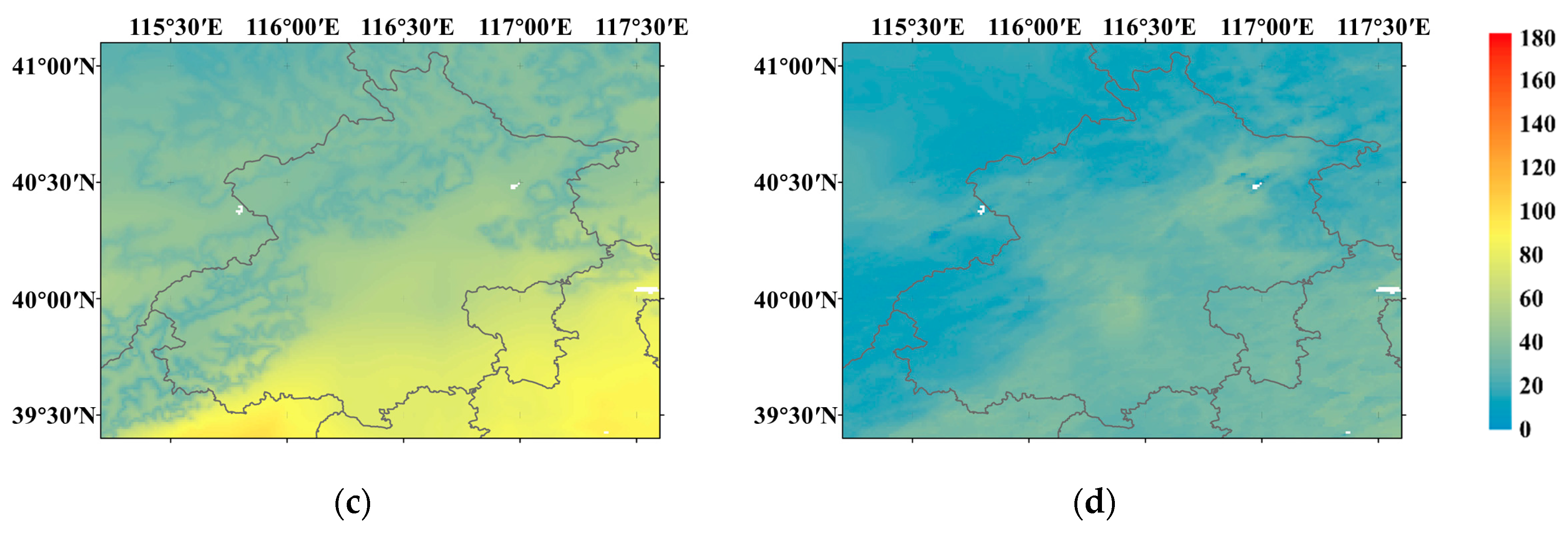
Figure 10 illustrates the monthly PM2.5 mass concentration in this study compared to the monthly PM2.5 mass concentration at 0.01° resolution published by Aaron van Donkelaar et al. [76]. The spatial distribution of PM2.5 is characterized similarly in both datasets, proving the reliability of the PM distribution in this study.
6. Conclusions
In this study, a virtual monitoring network for PM2.5/10 was established by a proportional relationship formula. The IGTWR model and refined measurement network were applied to AOD. Then a hybrid model was proposed, which was applied to AOD, meteorological data, time and space data, and land-use data to estimate PM2.5/10 mass concentrations in the study area at a spatial resolution of 100 m. The model results showed a reasonable spatial pattern similar to previous studies, with high values of PM2.5/10 occurring mainly in urban and southeastern suburbs, and lower values in the northern and western mountainous regions in Beijing. The estimation result of PM2.5 was validated by the ground stations with R2 ranging from 0.91 to 0.98 and the RMSE ranging from 4.51 μg/m3 to 17.04 μg/m3, and that for PM10 was validated by the ground stations with R2 ranging from 0.85 to 0.98 and the RMSE ranging from 6.98 µg/m3 to 29.00 µg/m3. This demonstrates the usability of the new hybrid model in the absence of sufficient AOD-monitoring data counterparts and provides a basis for future urban-scale PM estimates.
Despite these reliable results, some aspects of the model in this study could be improved. Firstly, the results of the model are influenced by the accuracy of the input AOD data, while the coverage of the results is also related to the AOD coverage. AOD data and meteorological field data with higher accuracy and resolution would benefit our model performance. Secondly, the temporal resolution of PM2.5/10 data affects the model performance [69]. Therefore, more time continuity in the AOD data was needed to improve model performance. Finally, as the association between ground-level PM2.5/10 and AOD is influenced by many different factors, more variables will be considered in our future studies (such as population density, road length, and emission information).
Author Contributions
Conceptualization, S.W., Y.S. and R.B.; methodology, S.W. and Y.S.; validation, S.W., Y.S. and R.B.; formal analysis, S.W.; investigation, Y.S.; resources, S.W., Y.S., R.B. and C.J.; data curation, S.W. and Y.S.; writing—original draft preparation, S.W. and Y.S.; writing—review and editing, Y.X. and Y.S.; visualization, Y.S.; supervision, Y.X. and X.J.; funding acquisition, Y.X. All authors have read and agreed to the published version of the manuscript.
Funding
This work was supported in part by the National Natural Science Foundation of China (NSFC) under Grant No. 42275147.
Data Availability Statement
Data are contained within the article.
Acknowledgments
The authors thank all data providers for their efforts in making the data available: the PM2.5/10 ground-based measurement data from the Chinese National Real-Time Air Quality Release Platform; BLH data from the European Centre for Medium-Range Weather Forecasts; RH data from the China National Meteorological Operational Intranet; land-use data from the Resource and Environment Data Cloud Platform; and AOD and PM2.5/10 simulation data from the CAMS (ECMWF Atmospheric Composition Reanalysis 4) global reanalysis.
Conflicts of Interest
The authors declare no conflict of interest.
References
- Beelen, R.; Raaschou-Nielsen, O.; Stafoggia, M.; Andersen, Z.J.; Weinmayr, G.; Hoffmann, B.; Wolf, K.; Samoli, E.; Fischer, P.; Nieuwenhuijsen, M.; et al. Effects of long-term exposure to air pollution on natural-cause mortality: An analysis of 22 European cohorts within the multicentre ESCAPE project. Lancet 2014, 383, 785–795. [Google Scholar] [CrossRef] [PubMed]
- Crouse, D.L.; Peters, P.A.; van Donkelaar, A.; Goldberg, M.S.; Villeneuve, P.J.; Brion, O.; Khan, S.; Atari, D.O.; Jerrett, M.; Pope, C.A.; et al. Risk of Non accidental and Cardiovascular Mortality in Relation to Long-term Exposure to Low Concentrations of Fine Particulate Matter: A Canadian National-Level Cohort Study. Environ. Health Perspect. 2012, 120, 708–714. [Google Scholar] [CrossRef] [PubMed]
- Dimitrova, R.; Lurponglukana, N.; Fernando, H.J.S.; Runger, G.C.; Hyde, P.; Hedquist, B.C.; Anderson, J.; Bannister, W.; Johnson, W. Relationship between particulate matter and childhood asthma – basis of a future warning system for central Phoenix. Atmos. Chem. Phys. 2012, 12, 2479–2490. [Google Scholar]
- Hoek, G.; Krishnan, R.M.; Beelen, R.; Peters, A.; Ostro, B.; Brunekreef, B.; Kaufman, J.D. Long-term air pollution exposure and cardio- respiratory mortality: A review. Environ. Health 2013, 12, 43. [Google Scholar] [CrossRef] [PubMed]
- Pascal, M.; Falq, G.; Wagner, V.; Chatignoux, E.; Corso, M.; Blanchard, M.; Host, S.; Pascal, L.; Larrieu, S. Short-term impacts of particulate matter (PM10, PM10–2.5, PM2.5) on mortality in nine French cities. Atmos. Environ. 2014, 95, 175–184. [Google Scholar] [CrossRef]
- Ballester, F.; Estarlich, M.; Iniguez, C.; Llop, S.; Ramon, R.; Esplugues, A.; Lacasana, M.; Rebagliato, M. Air pollution exposure during pregnancy and reduced birth size: A prospective birth cohort study in Valencia, Spain. Environ. Health 2010, 9, 6. [Google Scholar] [CrossRef] [PubMed]
- Lim, S.S.; Vos, T.; Flaxman, A.D.; Danaei, G.; Shibuya, K.; Adair-Rohani, H.; AlMazroa, M.A.; Amann, M.; Anderson, H.R.; Andrews, K.G.; et al. A comparative risk assessment of burden of disease and injury attributable to 67 risk factors and risk factor clusters in 21 regions, 1990–2010: A systematic analysis for the Global Burden of Disease Study 2010. Lancet 2012, 380, 2224–2260. [Google Scholar] [CrossRef] [PubMed]
- Rohde, R.A.; Muller, R.A. Air Pollution in China: Mapping of Concentrations and Sources. PLoS ONE 2015, 10, e0135749. [Google Scholar] [CrossRef]
- Geng, G.; Zhang, Q.; Martin, R.V.; van Donkelaar, A.; Huo, H.; Che, H.; Lin, J.; He, K. Estimating long-term PM2.5 concentrations in China using satellite-based aerosol optical depth and a chemical transport model. Remote Sens. Environ. 2015, 166, 262–270. [Google Scholar] [CrossRef]
- Peng, J.; Chen, S.; Lu, H.; Liu, Y.; Wu, J. Spatiotemporal patterns of remotely sensed PM2.5 concentration in China from 1999 to 2011. Remote Sens. Environ. 2016, 174, 109–121. [Google Scholar] [CrossRef]
- Hu, J.; Wang, Y.; Ying, Q.; Zhang, H. Spatial and temporal variability of PM2.5 and PM10 over the North China Plain and the Yangtze River Delta, China. Atmos. Environ. 2014, 95, 598–609. [Google Scholar] [CrossRef]
- Hu, X.; Waller, L.A.; Lyapustin, A.; Wang, Y.; Al-Hamdan, M.Z.; Crosson, W.L.; Estes, M.G.; Estes, S.M.; Quattrochi, D.A.; Puttaswamy, S.J.; et al. Estimating ground-level PM2.5 concentrations in the Southeastern United States using MAIAC AOD retrievals and a two-stage model. Remote Sens. Environ. 2014, 140, 220–232. [Google Scholar] [CrossRef]
- Qian, Z.; He, Q.; Lin, H.M.; Kong, L.; Bentley, C.M.; Liu, W.; Zhou, D. High Temperatures Enhanced Acute Mortality Effects of Ambient Particle Pollution in the “Oven” City of Wuhan, China. Environ. Health Perspect. 2008, 116, 1172–1178. [Google Scholar] [CrossRef]
- Hu, X.; Waller, L.A.; Lyapustin, A.; Wang, Y.; Liu, Y. 10-year spatial and temporal trends of PM2.5 concentrations in the southeastern US estimated using high-resolution satellite data. Atmos. Chem. Phys. 2014, 14, 6301–6314. [Google Scholar] [CrossRef]
- Lee, M.C.; Huang, N. Changes in self-perceived economic satisfaction and mortality at old ages: Evidence from a survey of middle-aged and elderly adults in Taiwan. Soc. Sci. Med. 2015, 130, 1–8. [Google Scholar] [CrossRef] [PubMed]
- Ma, Z.; Hu, X.; Huang, L.; Bi, J.; Liu, Y. Estimating Ground-Level PM2.5 in China Using Satellite Remote Sensing. Environ. Sci. Technol. 2014, 48, 7436–7444. [Google Scholar] [CrossRef]
- Zou, B.; Pu, Q.; Bilal, M.; Weng, Q.; Zhai, L.; Nichol, J.E. High-Resolution Satellite Mapping of Fine Particulates Based on Geographically Weighted Regression. IEEE Geosci. Remote Sens. Lett. 2016, 13, 495–499. [Google Scholar] [CrossRef]
- Engel-Cox, J.A.; Holloman, C.H.; Coutant, B.W.; Hoff, R.M. Qualitative and quantitative evaluation of MODIS satellite sensor data for regional and urban scale air quality. Atmos. Environ. 2004, 38, 2495–2509. [Google Scholar] [CrossRef]
- Schaap, M.; Apituley, A.; Timmermans, R.M.A.; Koelemeijer, R.B.A.; de Leeuw, G. Exploring the relation between aerosol optical depth and PM2.5 at Cabauw, the Netherlands. Atmos. Chem. Phys. 2009, 9, 909–925. [Google Scholar] [CrossRef]
- Hutchison, K.D.; Smith, S.; Faruqui, S.J. Correlating MODIS aerosol optical thickness data with ground-based PM2.5 observations across Texas for use in a real-time air quality prediction system. Atmos. Environ. 2005, 39, 7190–7203. [Google Scholar] [CrossRef]
- Liu, Y.; Sarnat, J.A.; Kilaru, V.; Jacob, D.J.; Koutrakis, P. Estimating Ground-Level PM2.5 in the Eastern United States Using Satellite Remote Sensing. Environ. Sci. Technol. 2005, 39, 3269–3278. [Google Scholar] [CrossRef]
- Kim, G.; Lee, S.; Im, J.; Song, C.K.; Kim, J.; Lee, M. Aerosol data assimilation and forecast using Geostationary Ocean Color Imager aerosol optical depth and in-situ observations during the KORUS-AQ observing period. Giscience Remote Sens. 2021, 58, 1175–1194. [Google Scholar] [CrossRef]
- Li, Y.; Xue, Y.; Guang, J.; She, L.; Fan, C.; Chen, G. Ground-Level PM2.5 Concentration Estimation from Satellite Data in the Beijing Area Using a Specific Particle Swarm Extinction Mass Conversion Algorithm. Remote Sens. 2018, 10, 1906. [Google Scholar] [CrossRef]
- Lin, C.; Li, Y.; Yuan, Z.; Lau, A.K.H.; Li, C.; Fung, J.C.H. Using satellite remote sensing data to estimate the high-resolution distribution of ground-level PM2.5. Remote Sens. Environ. 2015, 156, 117–128. [Google Scholar] [CrossRef]
- van Donkelaar, A.; Martin, R.V.; Brauer, M.; Boys, B.L. Use of Satellite Observations for Long-Term Exposure Assessment of Global Concentrations of Fine Particulate Matter. Environ. Health Perspect. 2015, 123, 135–143. [Google Scholar] [CrossRef] [PubMed]
- Zhang, X.; Chu, Y.; Wang, Y.; Zhang, K. Predicting daily PM2.5 concentrations in Texas using high-resolution satellite aerosol optical depth. Sci. Total Environ. 2018, 631–632, 904–911. [Google Scholar] [CrossRef]
- Gupta, P.; Christopher, S.A. Seven year particulate matter air quality assessment from surface and satellite measurements. Atmos. Chem. Phys. 2008, 8, 3311–3324. [Google Scholar] [CrossRef]
- Kloog, I.; Nordio, F.; Coull, B.A.; Schwartz, J. Incorporating Local Land Use Regression and Satellite Aerosol Optical Depth In A Hybrid Model Of Spatiotemporal PM2.5 Exposures In The Mid-Atlantic States. Environ. Sci. Technol. 2012, 46, 11913–11921. [Google Scholar] [CrossRef] [PubMed]
- Unnithan, S.L.K.; Gnanappazham, L. Spatiotemporal mixed effects modeling for the estimation of PM2.5 from MODIS AOD over the Indian subcontinent. Giscience Remote Sens. 2020, 57, 159–173. [Google Scholar] [CrossRef]
- He, Q.; Zhang, M.; Song, Y.; Huang, B. Spatiotemporal assessment of PM2.5 concentrations and exposure in China from 2013 to 2017 using satellite-derived data. J. Clean. Prod. 2021, 286, 124965. [Google Scholar] [CrossRef]
- Li, S.X.; Zou, B.; Fang, X.; Lin, Y. Time series modeling of PM2.5 concentrations with residual variance constraint in eastern mainland China during 2013–2017. Sci. Total Environ. 2020, 710, 135755. [Google Scholar] [CrossRef]
- Xue, W.H.; Zhang, J.; Zhong, C.; Ji, D.Y.; Huang, W. Satellite-derived spatiotemporal PM2.5 concentrations and variations from 2006 to 2017 in China. Sci. Total Environ. 2020, 712, 134577. [Google Scholar] [CrossRef]
- You, W.; Zang, Z.; Zhang, L.; Li, Y.; Wang, W. Estimating national-scale ground-level PM25 concentration in China using geographically weighted regression based on MODIS and MISR AOD. Environ. Sci. Pollut. Res. 2016, 23, 8327–8338. [Google Scholar] [CrossRef]
- Chen, G.; Knibbs, L.D.; Zhang, W.; Li, S.; Cao, W.; Guo, J.; Ren, H.; Wang, B.; Wang, H.; Williams, G.; et al. Estimating spatiotemporal distribution of PM1 concentrations in China with satellite remote sensing, meteorology, and land use information. Environ. Pollut. 2018, 233, 1086–1094. [Google Scholar] [CrossRef] [PubMed]
- Hua, Z.; Sun, W.; Yang, G.; Du, Q. A Full-Coverage Daily Average PM2.5 Retrieval Method with Two-Stage IVW Fused MODIS C6 AOD and Two-Stage GAM Model. Remote Sens. 2019, 11, 1558. [Google Scholar] [CrossRef]
- She, Q.; Choi, M.; Belle, J.H.; Xiao, Q.; Bi, J.; Huang, K.; Meng, X.; Geng, G.; Kim, J.; He, K.; et al. Satellite-based estimation of hourly PM2.5 levels during heavy winter pollution episodes in the Yangtze River Delta, China. Chemosphere 2020, 239, 124678. [Google Scholar] [CrossRef]
- Stafoggia, M.; Bellander, T.; Bucci, S.; Davoli, M.; de Hoogh, K.; de’Donato, F.; Gariazzo, C.; Lyapustin, A.; Michelozzi, P.; Renzi, M.; et al. Estimation of daily PM10 and PM2.5 concentrations in Italy, 2013–2015, using a spatiotemporal land-use random-forest model. Environ. Int. 2019, 124, 170–179. [Google Scholar] [CrossRef]
- Chen, W. Estimating PM2.5 with high-resolution 1-km AOD data and an improved machine learning model over Shenzhen, China. Sci. Total Environ. 2020, 746, 141093. [Google Scholar] [CrossRef] [PubMed]
- Guo, B.; Zhang, D.; Pei, L.; Su, Y.; Wang, X.; Bian, Y.; Zhang, D.; Yao, W.; Zhou, Z.; Guo, L. Estimating PM2.5 concentrations via random forest method using satellite, auxiliary, and ground-level station dataset at multiple temporal scales across China in 2017. Sci. Total Environ. 2021, 778, 146288. [Google Scholar] [CrossRef]
- Wei, J.; Li, Z.; Xue, W.; Sun, L.; Fan, T.; Liu, L.; Su, T.; Cribb, M. The ChinaHighPM10 dataset: Generation, validation, and spatiotemporal variations from 2015 to 2019 across China. Environ. Int. 2021, 146, 106290. [Google Scholar] [CrossRef] [PubMed]
- Jung, C.R.; Hwang, B.F.; Chen, W.T. Incorporating long-term satellite-based aerosol optical depth, localized land use data, and meteorological variables to estimate ground-level PM2.5 concentrations in Taiwan from 2005 to 2015. Environ. Pollut. 2018, 237, 1000–1010. [Google Scholar] [CrossRef]
- Xu, Y.; Ho, H.C.; Wong, M.S.; Deng, C.; Shi, Y.; Chan, T.C.; Knudby, A. Evaluation of machine learning techniques with multiple remote sensing datasets in estimating monthly concentrations of ground-level PM2.5. Environ. Pollut. 2018, 242, 1417–1426. [Google Scholar] [CrossRef]
- Chen, B.; You, S.; Ye, Y.; Fu, Y.; Ye, Z.; Deng, J.; Wang, K.; Hong, Y. An interpretable self-adaptive deep neural network for estimating daily spatially-continuous PM2.5 concentrations across China. Sci. Total Environ. 2021, 768, 144724. [Google Scholar] [CrossRef] [PubMed]
- Li, T.; Shen, H.; Zeng, C.; Yuan, Q.; Zhang, L. Point-surface fusion of station measurements and satellite observations for mapping PM2.5 distribution in China: Methods and assessment. Atmos. Environ. 2017, 152, 477–489. [Google Scholar] [CrossRef]
- Zang, L.; Mao, F.; Guo, J.; Wang, W.; Pan, Z.; Shen, H.; Zhu, B.; Wang, Z. Estimation of spatiotemporal PM1.0 distributions in China by combining PM2.5 observations with satellite aerosol optical depth. Sci. Total Environ. 2019, 658, 1256–1264. [Google Scholar] [CrossRef]
- Song, W.; Jia, H.; Huang, J.; Zhang, Y. A satellite-based geographically weighted regression model for regional PM2.5 estimation over the Pearl River Delta region in China. Remote Sens. Environ. 2014, 154, 1–7. [Google Scholar] [CrossRef]
- He, Q.; Huang, B. Satellite-based high-resolution PM2.5 estimation over the Beijing-Tianjin-Hebei region of China using an improved geographically and temporally weighted regression model. Environ. Pollut. 2018, 236, 1027–1037. [Google Scholar] [CrossRef] [PubMed]
- Liu, K.; Wu, Y.; Wang, X.; Wang, C. Impact of the spatial structure of urban agglomerations on air pollution in China. China Popul.·Resour. Environ. 2020, 30, 28–35. [Google Scholar]
- Huo, F.; Xu, L.; Li, Y.; Famiglietti, J.S.; Li, Z.; Kajikawa, Y.; Chen, F. Using big data analytics to synthesize research domains and identify emerging fields in urban climatology. Wiley Interdiscip. Rev. Clim. Chang. 2021, 12, e688. [Google Scholar] [CrossRef]
- Sun, K.; Chen, X.; Zhu, Z.; Zhang, T. High Resolution Aerosol Optical Depth Retrieval Using Gaofen-1 WFV Camera Data. Remote Sens. 2017, 9, 89. [Google Scholar] [CrossRef]
- Zhang, T.; Zhu, Z.; Gong, W.; Zhu, Z.; Sun, K.; Wang, L.; Huang, Y.; Mao, F.; Shen, H.; Li, Z.; et al. Estimation of ultrahigh resolution PM2.5 concentrations in urban areas using 160 m Gaofen-1 AOD retrievals. Remote Sens. Environ. 2018, 216, 91–104. [Google Scholar] [CrossRef]
- Bai, R.; Xue, Y.; Jiang, X.; Jin, C.; Sun, Y. Retrieval of High-Resolution Aerosol Optical Depth for Urban Air Pollution Monitoring. Atmosphere 2022, 13, 756. [Google Scholar] [CrossRef]
- Han, L.; Zhou, W.; Li, W.; Li, L. Impact of urbanization level on urban air quality: A case of fine particles (PM2.5) in Chinese cities. Environ. Pollut. 2014, 194, 163–170. [Google Scholar] [CrossRef] [PubMed]
- Van Donkelaar, A.; Martin, R.V.; Brauer, M.; Kahn, R.; Levy, R.; Verduzco, C.; Villeneuve, P.J. Global Estimates of Ambient Fine Particulate Matter Concentrations from Satellite-Based Aerosol Optical Depth: Development and Application. Environ. Health Perspect. 2010, 118, 847–855. [Google Scholar] [CrossRef]
- Xu, X.; Liu, J.; Zhuang, D. Remote sensing Monitoring methods of land use/cover changes in national scale. Anhui Agric. Sci. 2012, 40, 2365–2369. [Google Scholar]
- Li, Z.; Shen, H.; Li, H.; Xia, G.; Gamba, P.; Zhang, L. Multi-feature combined cloud and cloud shadow detection in GaoFen-1 wide field of view imagery. Remote Sens. Environ. 2017, 191, 342–358. [Google Scholar] [CrossRef]
- Johnson, K.; Cole-Rhodes, A.; Zavorin, I.; Le Moigne, J. Mutual information as a similarity measure for remote sensing image registration. Geo-Spat. Image Data Exploit. II 2001, 4383, 51–61. [Google Scholar]
- Li, Y.; Xue, Y.; He, X.; Guang, J. High-resolution aerosol remote sensing retrieval over urban areas by synergetic use of HJ-1 CCD and MODIS data. Atmos. Environ. 2012, 46, 173–180. [Google Scholar] [CrossRef]
- Xue, Y.; He, X.W.; Xu, H.; Guang, J.; Guo, J.P.; Mei, L.L. China Collection 2.0: The aerosol optical depth dataset from the synergetic retrieval of aerosol properties algorithm. Atmos. Environ. 2014, 95, 45–58. [Google Scholar] [CrossRef]
- Xue, Y.; Cracknell, A.P. Operational bi-angle approach to retrieve the Earth surface albedo from AVHRR data in the visible band. Remote Sens. 1995, 16, 417–429. [Google Scholar] [CrossRef]
- Xue, Y.; Li, Y.; Guang, J.; Tugui, A.; She, L.; Qin, K.; Fan, C.; Che, Y.; Xie, Y.; Wen, Y.; et al. Hourly PM2.5 Estimation over Central and Eastern China Based on Himawari-8 Data. Remote Sens. 2020, 12, 855. [Google Scholar] [CrossRef]
- Shin, M.; Kang, Y.; Park, S.; Im, J.; Yoo, C.; Quackenbush, L.J. Estimating ground-level particulate matter concentrations using satellite-based data: A review. Giscience Remote Sens. 2020, 57, 174–189. [Google Scholar] [CrossRef]
- Liu, Y.; Park, R.J.; Jacob, D.J.; Li, Q.B.; Kilaru, V.; Sarnat, J.A. Mapping annual mean ground-level PM2.5 concentrations using Multiangle Imaging Spectroradiometer aerosol optical thickness over the contiguous United States. J. Geophys. Res.-Atmos. 2004, 109, 10. [Google Scholar] [CrossRef]
- Huang, B.; Wu, B.; Barry, M. Geographically and temporally weighted regression for modeling spatio-temporal variation in house prices. Int. J. Geogr. Inf. Sci. 2010, 24, 383–401. [Google Scholar] [CrossRef]
- Pugh, T.A.M.; MacKenzie, A.R.; Whyatt, J.D.; Hewitt, C.N. Effectiveness of Green Infrastructure for Improvement of Air Quality in Urban Street Canyons. Environ. Sci. Technol. 2012, 46, 7692–7699. [Google Scholar] [CrossRef] [PubMed]
- Sun, Y.; Xue, Y.; Jiang, X.; Jin, C.; Wu, S.; Zhou, X. Estimation of the PM2.5 and PM10 Mass Concentration over Land from FY-4A Aerosol Optical Depth Data. Remote Sens. 2021, 13, 4276. [Google Scholar] [CrossRef]
- Wu, J.; Yao, F.; Li, W.; Si, M. VIIRS-based remote sensing estimation of ground-level PM2.5 concentrations in Beijing–Tianjin–Hebei: A spatiotemporal statistical model. Remote Sens. Environ. 2016, 184, 316–328. [Google Scholar] [CrossRef]
- Miao, Y.; Liu, S.; Guo, J.; Huang, S.; Yan, Y.; Lou, M. Unraveling the relationships between boundary layer height and PM2.5 pollution in China based on four-year radiosonde measurements. Environ. Pollut. 2018, 243, 1186–1195. [Google Scholar] [CrossRef]
- Guo, Y.; Tang, Q.; Gong, D.Y.; Zhang, Z. Estimating ground-level PM2.5 concentrations in Beijing using a satellite-based geographically and temporally weighted regression model. Remote Sens. Environ. 2017, 198, 140–149. [Google Scholar] [CrossRef]
- Zhang, Y.; Li, Z. Remote sensing of atmospheric fine particulate matter (PM2.5) mass concentration near the ground from satellite observation. Remote Sens. Environ. 2015, 160, 252–262. [Google Scholar] [CrossRef]
- Guo, Y.; Feng, N.; Christopher, S.A.; Kang, P.; Zhan, F.B.; Hong, S. Satellite remote sensing of fine particulate matter (PM2.5) air quality over Beijing using MODIS. Int. J. Remote Sens. 2014, 35, 6522–6544. [Google Scholar] [CrossRef]
- Li, R.; Gong, J.; Chen, L.; Wang, Z. Estimating Ground-Level PM2.5 Using Fine-Resolution Satellite Data in the Megacity of Beijing, China. Aerosol Air Qual. Res. 2015, 15, 1347–1356. [Google Scholar] [CrossRef]
- Liu, Y.; Servant, A.; Guy, O.J.; Al-Jamal, K.T.; Williams, P.R.; Hawkins, K.M.; Kostarelos, K. An electric-field responsive microsystem for controllable miniaturised drug delivery applications. Sens. Actuators B Chem. 2012, 175, 100–105. [Google Scholar] [CrossRef]
- Xie, Y.; Wang, Y.; Zhang, K.; Dong, W.; Lv, B.; Bai, Y. Daily Estimation of Ground-Level PM2.5 Concentrations over Beijing Using 3 km Resolution MODIS AOD. Environ. Sci. Technol. 2015, 49, 12280–12288. [Google Scholar] [CrossRef]
- Xin, J.; Zhang, Q.; Wang, L.; Gong, C.; Wang, Y.; Liu, Z.; Gao, W. The empirical relationship between the PM2.5 concentration and aerosol optical depth over the background of North China from 2009 to 2011. Atmos. Res. 2014, 138, 179–188. [Google Scholar] [CrossRef]
- van Donkelaar, A.; Hammer, M.S.; Bindle, L.; Brauer, M.; Brook, J.R.; Garay, M.J.; Hsu, N.C.; Kalashnikova, O.V.; Kahn, R.A.; Lee, C.; et al. Monthly Global Estimates of Fine Particulate Matter and Their Uncertainty. Environ. Sci. Technol. 2021, 55, 15287–15300. [Google Scholar] [CrossRef]
Figure 1.
Study areas with the land types and locations of the air quality monitoring stations. Please refer to the Table 1 for the detailed information of land-use types.
Figure 1.
Study areas with the land types and locations of the air quality monitoring stations. Please refer to the Table 1 for the detailed information of land-use types.

Figure 2.
The workflow of proportional relationship formula (top box), improved geographically and temporally weighted regression (IGTWR) model (middle box), and model validation (bottom box).
Figure 2.
The workflow of proportional relationship formula (top box), improved geographically and temporally weighted regression (IGTWR) model (middle box), and model validation (bottom box).

Figure 3.
Flow chart for refined PM2.5/10 monitoring stations using proportional relationship formula and other data.
Figure 3.
Flow chart for refined PM2.5/10 monitoring stations using proportional relationship formula and other data.

Figure 4.
The distribution levels of seasonal mean PM2.5 mass concentrations at 100 m resolution estimated by the model are shown for spring/summer/autumn/winter, (a), (b), (c), and (d), respectively. The monthly mean PM10 mass concentration distribution levels for spring/summer/autumn/winter are shown at 100 m resolution for the model estimates, (e), (f), (g), and (h), respectively. Estimates of PM2.5/10 are missing at the eastern margin component due to insufficient matching of GF data.


Figure 5.
Model-estimated distribution levels of annual PM2.5 (a) and PM10 (b) mass concentrations at 100 m resolution. Estimates of PM2.5/10 are missing in the eastern margin component due to insufficient matching of GF data.
Figure 5.
Model-estimated distribution levels of annual PM2.5 (a) and PM10 (b) mass concentrations at 100 m resolution. Estimates of PM2.5/10 are missing in the eastern margin component due to insufficient matching of GF data.

Figure 6.
Distribution of PM2.5 and PM10 mass concentrations (µm/m3) at hourly resolution for clear and high pollution dates. The first row is PM2.5 and the second row is PM10, from left to right. Each column has the same time parameter, 14:00 on 12 April 2020 (a,e), 10:00 on 28 April 2020 (b,f), 14:00 on 28 April 2020 (c,g), and 10:00 on 5 June 2020 (d,h). The times are local standard time.

Figure 7.
Cross-validation results for spring (a) summer (b) autumn (c) winter (d) based on the GWC model for PM2.5. Cross-validation results for spring (e) summer (f) autumn (g) winter (h) based on the GWR model for PM2.5. The solid black line is the 1:1 reference line.
Figure 7.
Cross-validation results for spring (a) summer (b) autumn (c) winter (d) based on the GWC model for PM2.5. Cross-validation results for spring (e) summer (f) autumn (g) winter (h) based on the GWR model for PM2.5. The solid black line is the 1:1 reference line.


Figure 8.
Cross-validation results for spring (a), summer (b), autumn (c), and winter (d) based on the GWC model for PM10. Cross-validation results for spring (e), summer (f), autumn (g), and winter (h) based on the GWR model for PM10.The solid black line is the 1:1 reference line.
Figure 8.
Cross-validation results for spring (a), summer (b), autumn (c), and winter (d) based on the GWC model for PM10. Cross-validation results for spring (e), summer (f), autumn (g), and winter (h) based on the GWR model for PM10.The solid black line is the 1:1 reference line.


Figure 9.
Validation of PM2.5 mass concentrations calculated using the RPF against ground stations (a). Validation of PM10 mass concentrations calculated using the RPF against ground stations (b). The solid black line is the 1:1 reference line.
Figure 9.
Validation of PM2.5 mass concentrations calculated using the RPF against ground stations (a). Validation of PM10 mass concentrations calculated using the RPF against ground stations (b). The solid black line is the 1:1 reference line.

Figure 10.
Distribution of monthly PM2.5 mass concentrations at 100 m resolution (a,b) compared to the monthly PM2.5 product (c,d) published by Aaron van Donkelaar et al. [76]. The left column is for January and the right is for April.
Figure 10.
Distribution of monthly PM2.5 mass concentrations at 100 m resolution (a,b) compared to the monthly PM2.5 product (c,d) published by Aaron van Donkelaar et al. [76]. The left column is for January and the right is for April.


Table 1.
The land-use types in China [55].
Table 1.
The land-use types in China [55].
| Number | Designation | Number | Designation | Number | Designation |
|---|---|---|---|---|---|
| 11 | Paddy field | 41 | Channel | 61 | Sand |
| 12 | Dry land | 42 | Lake | 62 | Gobi |
| 21 | Woodland | 43 | Reservoir pond | 63 | Saline alkali soil |
| 22 | Shrub wood | 44 | Permanent glacier and snow | 64 | Swamp land |
| 23 | Sparse woodland | 45 | Tidal flat | 65 | Bare land |
| 24 | Other woodlands | 46 | Beach land | 66 | Bare rock texture |
| 31 | High-coverage grassland | 51 | Urban land use | 67 | Other |
| 32 | Medium-coverage grassland | 52 | Rural settlements | 99 | Undefined |
| 33 | Low-coverage grassland | 53 | Other construction land |
Table 2.
Definitions of terms used in this analysis.
| Term | Unit | Definition |
|---|---|---|
| Simulated PM2.5 concentration | mg/m3 | PM2.5 or PM10 provided by CAMS, verification results with the 12 monitoring stations of the Ministry of Environmental Protection (MEP) within Beijing in 2020 show that the average R values are 0.59 and 0.43, respectively (https://cams2-82.aeroval.met.no/, accessed on 27 January 2024). |
| Simulated AOD | unitless | AOD provided by CAMS, verification results with the AeronetL1.5-d of Beijing station in 2020 show that the R and R2 values are 0.80 and 0.89, respectively (https://cams2-82.aeroval.met.no/, accessed on 27 January 2024). |
| GF AOD | unitless | The TERRA and AQUA satellite MODIS data were first downscaled by GF-1 WFV data, then calculated the AOD by the SRAP algorithm. |
| GF PRF PM2.5/10 concentration | µg/m3 | PM2.5 or PM10 concentrations at 10:00 or 14:00 local time. |
Table 3.
Model performance using refined and unrefined site networks modeled separately, and coverage of results by different methods.
Table 3.
Model performance using refined and unrefined site networks modeled separately, and coverage of results by different methods.
| Method | R2/RMSE | Coverage |
|---|---|---|
| PM2.5 GWC | 0.778/34.702 µg/m3 | 92.91% |
| PM2.5 GWR | 0.660/25.434 µg/m3 | 40.73% |
| PM10 GWC | 0.741/49.757 µg/m3 | 92.95% |
| PM10 GWR | 0.550/38.052 µg/m3 | 40.93% |
Disclaimer/Publisher’s Note: The statements, opinions and data contained in all publications are solely those of the individual author(s) and contributor(s) and not of MDPI and/or the editor(s). MDPI and/or the editor(s) disclaim responsibility for any injury to people or property resulting from any ideas, methods, instructions or products referred to in the content. |
© 2024 by the authors. Licensee MDPI, Basel, Switzerland. This article is an open access article distributed under the terms and conditions of the Creative Commons Attribution (CC BY) license (https://creativecommons.org/licenses/by/4.0/).
Share and Cite
MDPI and ACS Style
Wu, S.; Sun, Y.; Bai, R.; Jiang, X.; Jin, C.; Xue, Y. Estimation of PM2.5 and PM10 Mass Concentrations in Beijing Using Gaofen-1 Data at 100 m Resolution. Remote Sens. 2024, 16, 604. https://doi.org/10.3390/rs16040604
AMA Style
Wu S, Sun Y, Bai R, Jiang X, Jin C, Xue Y. Estimation of PM2.5 and PM10 Mass Concentrations in Beijing Using Gaofen-1 Data at 100 m Resolution. Remote Sensing. 2024; 16(4):604. https://doi.org/10.3390/rs16040604
Chicago/Turabian StyleWu, Shuhui, Yuxin Sun, Rui Bai, Xingxing Jiang, Chunlin Jin, and Yong Xue. 2024. "Estimation of PM2.5 and PM10 Mass Concentrations in Beijing Using Gaofen-1 Data at 100 m Resolution" Remote Sensing 16, no. 4: 604. https://doi.org/10.3390/rs16040604
Note that from the first issue of 2016, this journal uses article numbers instead of page numbers. See further details here.