
Estimating Winter Arctic Sea Ice Motion Based on Random Forest Models

1
School of Atmospheric Sciences, Sun Yat-sen University and Southern Marine Science and Engineering Guangdong Laboratory (Zhuhai), Zhuhai 519082, China
2
Institute for Atmospheric and Earth System Research, University of Helsinki, 00014 Helsinki, Finland
*
Author to whom correspondence should be addressed.
Remote Sens. 2024, 16(3), 581; https://doi.org/10.3390/rs16030581
Submission received: 16 December 2023
/
Revised: 25 January 2024
/
Accepted: 1 February 2024
/
Published: 3 February 2024
(This article belongs to the Special Issue Remote Sensing of Polar Sea Ice)
Abstract
:Sea ice motion (SIM) plays a crucial role in setting the distribution of the ice cover in the Arctic. Limited by images’ spatial resolution and tracking algorithms, challenges exist in obtaining coastal sea ice motion (SIM) based on passive microwave satellite sensors. In this study, we developed a method based on random forest (RF) models to obtain Arctic SIM in winter by incorporating wind field and coastal geographic location information. These random forest models were trained using Synthetic Aperture Radar (SAR) SIM data. Our results show good consistency with SIM data retrieved from satellite imagery and buoy observations. With respect to the SAR data, compared with SIM estimated with RF model training using reanalysis surface wind, the results by additional coastal information input had a lower root mean square error (RMSE) and a higher correlation coefficient by 31% and 14% relative improvement, respectively. The latter SIM result also showed a better performance for magnitude, especially within 100 km of the coastline in the north of the Canadian Arctic Archipelago. In addition, the influence of coastline on SIM is quantified through variable importance calculation, at 22% and 28% importance of all RF variables for east and north SIM components, respectively. These results indicate the great potential of RF models for estimating SIM over the whole Arctic Ocean in winter.
1. Introduction
Sea ice motion (SIM) is largely controlled by winds and ocean currents and is also affected by sea ice internal stress and the Coriolis force. The influence of coastal conditions on sea ice drift can be conveyed through internal friction when the ice field is compact. The shape of the coastline also affects the ocean currents that further modify the motion of sea ice [1,2,3,4]. The differential sea ice velocity causes deformation including the opening and closing of leads, which affects not only the mass balance of sea ice but also the spatial variation in the latent and sensible heat fluxes in the Arctic Ocean [5].
At present, sea ice motion data based on microwave imagery are the most extensively utilized data for studying the drift of sea ice in the polar regions [6,7,8]. Due to the limitations of image resolution and algorithms, the existing passive microwave SIM products typically do not cover the sea area 100–150 km from the coastline. In recent years, high-resolution Synthetic Aperture Radar (SAR) SIM datasets have gradually become an important source of high-resolution sea ice motion features [9,10,11]. While SAR ice velocity data can include coastal ice motion, they are limited by their spatial and temporal coverage. Additionally, in near-shore areas, due to the interaction between sea ice and shore, sea ice drift is slower than further offshore [3], which makes it difficult for satellite tracking methods to estimate ice motion. Therefore, challenges remain in obtaining SIM over the whole Arctic Ocean through satellite remote sensing methods.
In addition to extracting ice motion from consecutive satellite images, it can be directly estimated from surface wind data [8,12]. However, such SIM data cannot accurately reflect the dynamics of sea ice under the impact of internal friction, ocean currents, and coastal boundaries [3,8]. In recent years, machine learning (ML) methods have been shown to have great potential for sea ice motion estimation and prediction [13,14,15,16]. For example, Palerme and Müller (2021) [14] reproduced the result that the wind field is the most important factor affecting the Arctic ice speed, and the influence of parameters related to sea ice and shore boundaries cannot be ignored since they accounted for 20–30% of the variable importances (for the concept of importance in RF models, see [17]). in addition, Hoffman et al. (2023) [16] compared the performance of persistence (PS), linear regression (LR), and a convolutional neural network (CNN) model, and found that different machine learning methods have better SIM estimation and prediction quality in areas far from the coast than in near-shore areas. But to our knowledge, the impact of shore boundaries on SIM has not yet been quantitatively considered.
In this study, we employed a random forest model to generate Arctic sea ice motion with only wind and coastline forcing parameters as the input variables. We used the random forest method to estimate SIM because it has been successfully used in previous works and can quantify the contributions of different input variables. This article aimed to obtain the pan-Arctic covered sea ice motion data over the Arctic Ocean with a particular focus on reducing the uncertainties in the coastal area. The remainder of this paper is organized as follows: Section 2 and Section 3 introduce the data used and the random forest model. The evaluation and comparison of the results are presented in Section 4. The limitations of this study are discussed in Section 5. Finally, the conclusions are presented in Section 6.
2. Data
2.1. Target and Input Variables for the RF Model
2.1.1. The Target Variable
The daily gridded sea ice drift derived from Sentinel-1 SAR imagery (SEAICE_GLO_SEAICE_L4_NRT_OBSERVATIONS _011_006) distributed by Copernicus Marine Service (CMEMS) was used as the target SIM for the training of the random forest model and as the reference dataset for verification in this study (Table 1). It has a 10 km spatial resolution and one-day temporal resolution from daily data at 12:00 UTC. Although there are inconsistencies with buoy SIM data [14], SAR SIM data are still the optimum for random forest model training, mainly due to the most abundant near-shore SIM data.
2.1.2. Input Variables
This study divided the input variables into two categories: wind variables and coastline parameters (Table 1). Firstly, given that the wind field is a key factor influencing sea ice motion [18,19,20], we utilized 6-h wind field data from the European Centre for Medium-Range Weather Forecasts (ECMWF) ERA5 10 m wind speed data [21].
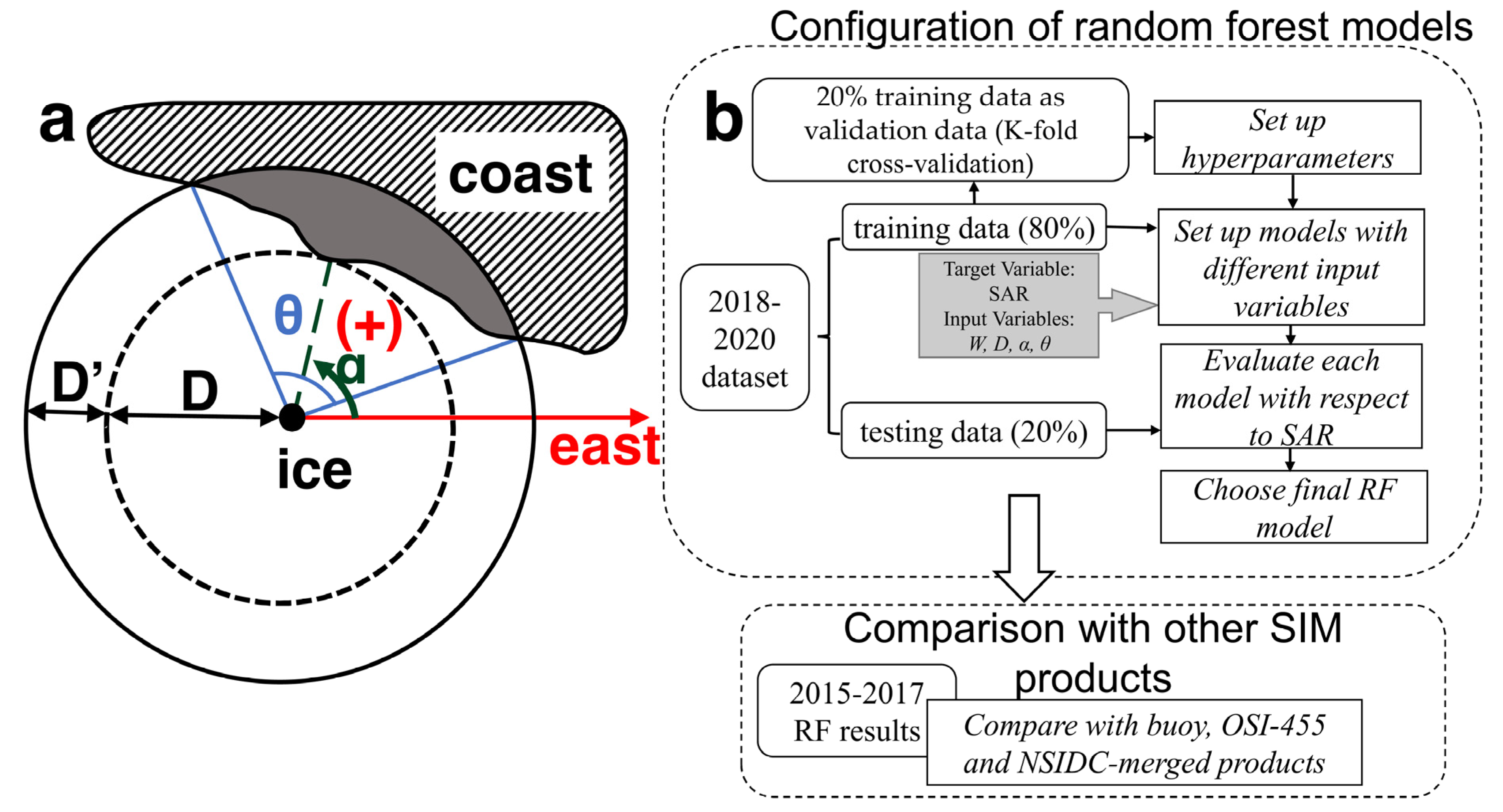
Secondly, in the representation of coastal effects, we introduced three parameters for each drift ice parcel (Figure 1a): (1) the distance to the nearest coastline (D); (2) the azimuth angle of coastline (α) that is the counterclockwise angle from east axis to the line connecting the nearest point of the ice pack at the shore boundary; and (3) the distance between the farthest and closest points that can affect SIM (D′) and sector angle (θ) of effective coastline that is an approximation of the extent width of the coastline that influence the SIM. Among these parameters, the maximum extent width (D′) is used to determine the width range of the coastal influence on ice. Then, the sector angle (θ) of sea ice and the coast is set within the range of D + D′. In this study, the values of D′ are 10 km, 30 km, 50 km, 70 km, and 90 km. The coastline used in this article was extracted from the ocean bathymetry used by a coupled ocean-sea ice data assimilation system for the North Atlantic Ocean and Arctic in the TOPAZ4 prediction system [22].
2.2. Comparison Datasets
Sea ice motion derived from buoy positions of the International Arctic Buoy Program (IABP, data available at https://iabp.apl.uw.edu/data.html, accessed on 31 January 2024) was used here to evaluate and compare with the SIM results derived from RF models. We also used a newly distributed multi-sensor low-resolution sea ice motion dataset from the Ocean and Sea Ice Satellite Application Facility (OSI SAF), which is based on Passive Microwave Radiometer data (SSM/I, SSMIS, AMSR-E, and AMSR2). This dataset has a 75 km spatial resolution and a one-day time interval. It is referred to as OSI-455 hereafter. Meanwhile, the National Snow and Ice Data Center (NSIDC) Polar Pathfinder Daily 25 km EASE-Grid Sea Ice Motion Vectors, Version 4 data, which provides daily sea ice motion in the polar regions with a spatial resolution of 25 km, were used for verification as well. This daily NSIDC sea ice motion product (referred to as NSIDC-merged hereafter) merges several types of data such as gridded satellite imagery (AVHRR, AMSR-E, SMMR, SSM/I, and SSMIS), data from the International Arctic Buoy Program, and surface winds from NCEP/NCAR Reanalysis.
SIM variations are dominated by the surface wind [18], so wind-derived SIM is an important supplement to satellite SIM observations, especially when satellite observations are missing. Here, we considered two types of SIM derived solely from wind. One was from NSIDC v4 based on NCEP/NCAR wind data (called NCEP-W), and it was estimated under the assumption that the sea ice speed is approximately 1% of the surface wind speed with a turning angle of about 20 degrees right to the wind following the results of Thorndike and Colony with a reduced wind factor [18]. The second wind-derived SIM was estimated from ERA5 10 m wind data using the same assumption as [18], with SIM speed equal to 2% of surface speed and SIM direction 20 degrees to the right from the wind (referred to as ERA5-W).
3. Methods
3.1. Configuration of Random Forest Models
Random forests (RF) is a machine learning algorithm commonly used for classification and regression tasks [23]. It is an ensemble method that combines multiple decision trees to make predictions. Here, the random forest regression model of the Python library scikit-learn 1.3.0 [24] was used. Figure 1b shows the process flow of the approach used in this paper. Two sets of models for the eastward and northward components were separately developed using SAR data as the target variable. The quality of the split nodes was measured using Friedman’s mean squared error as the standard.
Hyperparameters are used to control the learning process of an RF model. K-fold cross-validation is a method for assessing the performance of a model that involves splitting the dataset into k subsets or “folds” (here, k = 10), with each part/fold serving as the validation set in turn with the remaining parts serving as the training set. This study used the k-fold cross-validation method to conduct a sensitivity analysis of hyperparameters (Section 3.4). We adopted the Palerme and Müller (2021) [14] methods to train random forest models utilizing validation data from 80% of the training dates (16% of the total dataset, as displayed in Figure 1b), which were randomly chosen within the training periods. The remaining 84% of the dates were then employed to assess the model’s performance. This process was repeated ten times, and each time, the average mean absolute error (MAE) of the ten models was used to evaluate the quality of the hyperparameters. The performance of each model was averaged over the ten iterations to provide a more robust estimate.
The result of a random forest regressor is the mean value of the results from all decision trees. Thus, a property of the RF algorithm is that it tends to predict fewer extreme values than the target variable has because the mean value from all decision trees is used as the prediction, making it difficult to generate extremely low and high SIM magnitudes.
3.2. Constructing Training DatasetDatasets
Since sea ice melts and opens in summer in the Arctic, it is in a free drift state and less affected by the coastline. Therefore, the study period of this article focused on consolidated sea ice in the Arctic Ocean during the freezing period. Similar to Palerme and Müller (2021) [14], the data during the winter months (December to April) of 2018 to 2020 were taken into consideration. November was excluded because typically then Arctic Ocean is not yet fully covered by sea ice during November (Chukchi Sea is still open), which differs from the main applicable range of our model (winter full sea ice cover). The dataset was randomly divided, with 80% designated as the training data and the remaining 20% designated for model evaluation as the testing data. To maintain consistency, all models were trained using the same training period. In addition, because of the large length scale of dynamics of compact sea ice and the high spatial resolution of SAR SIM, the speed of sea ice at nearby grid points showed a strong correlation. Considering all the grid points where SAR observations were accessible after interpolating into 12.5 km grids could lead to the use of numerous highly correlated points for model training, increasing the risk of overfitting (which means when models capture the noise in the training data, resulting in worse performance). Palerme and Müller (2021) suggested that using 2% leads to the best performance [14]. Hence, this study employed the same proportion. We also excluded the Canadian Arctic Archipelago (CAA) area because there the SIM is largely influenced by the presence of narrow channels and land boundaries instead of surface wind.
3.3. Method of Evaluation
In addition to the normal measures, including bias, mean absolute error (MAE), root mean squared error (RMSE), and correlation (r), for the evaluation of SIM data, we also took skill [15,16,25] into consideration, which was calculated as follows:
where x and y indicate observations and prediction values, respectively. Further, in Section 4.2, we converted the eastward and northward components into magnitude and direction to find how the coastline parameters affect the SIM results. The magnitude of sea ice drift in the two datasets was straightforward, but due to the circular nature of the directional data when comparing the direction of sea ice drift in the different datasets, we followed the method described by Equation (2), in which Θx and Θy are directions with the subscripts x and y representing observations and predictions, respectively, and
Here, to measure the contribution of each input variable in the total model, the variable importance is used. The numerical value of the importance of each input variable is calculated as the (normalized) total reduction in the Gini index, which is a measure of homogeneity in the data, brought by the given variable [24].
3.4. Sensitivity Experiments of Hyperparameters and Setting up Input Variables
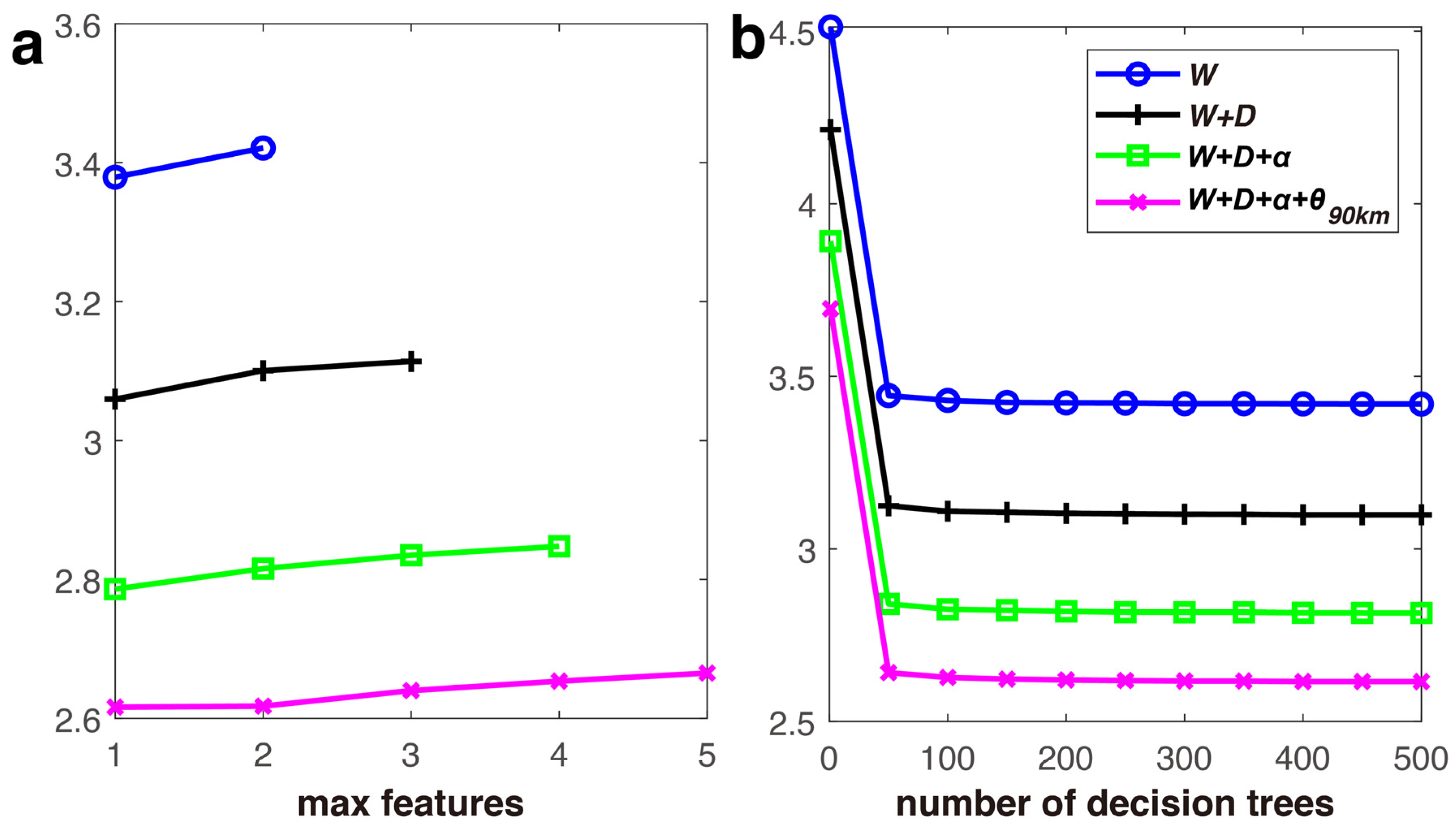
In this section, k-fold cross-validation was first used to identify the optimal hyperparameters for various input parameters. The number of decision trees and max features were optimized. The max features parameter determines the number of features considered when looking for the optimal split point in a decision tree (Figure 2a). An RF model uses all the input variables but only considers the number of ‘max features’ input variables for node splitting. MAE monotonically decreases with the increase in the number of decision trees (Figure 2b). After 100, the increase in the number of decision trees has little impact on MAE. In order to balance the computational efficiency and a relatively low MAE, we used 300 decision trees for all sensitivity experiments of the input variables (there were no significant improvements when using more trees). As for the max features, the number was set to 1 for experiments including ERA5 surface wind (W), wind and distance (W + D), wind, distance, and azimuth angle (W + D + α) as the input variables, and it was set to 2 in the case of experiments that incorporated θ (W + D + α + θ), as in each case their MAE values were the lowest (Figure 2a). Since the hyperparameters for the scenarios with different distances (10 km, 30 km, 50 km, 70 km, and 90 km) were essentially the same, only the results for the 90 km scenario are presented here.
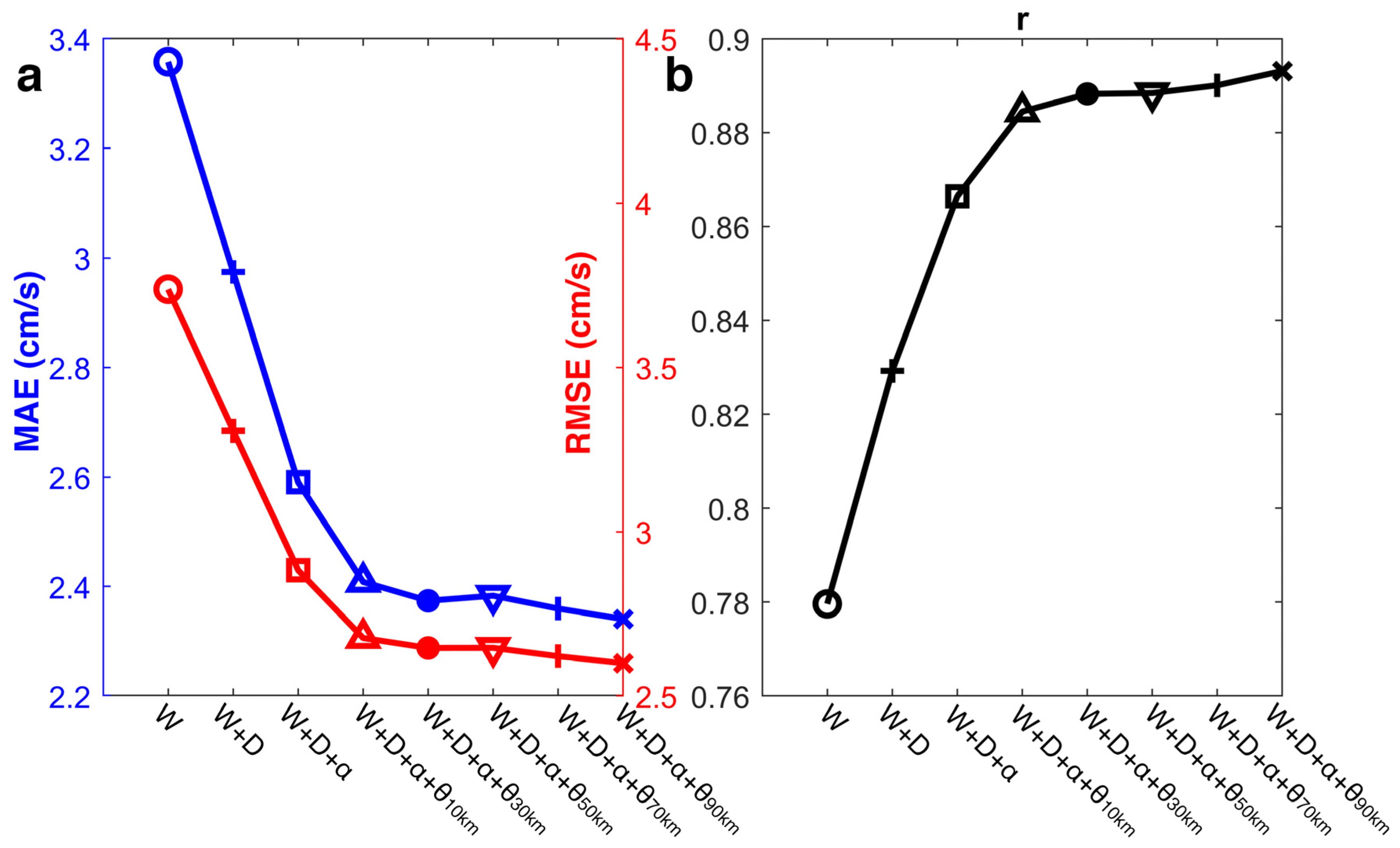
Subsequently, the impact of the different input variables was assessed using the remaining 20% of the data (testing data) apart from 80% training data of the total SAR data. This allowed us to evaluate the performance of the results when incorporating different input variables. The process of adding input variables reduced the overall MAE and RMSE and increased the correlation, as displayed in Figure 3. When the boundary parameters were taken into account, the MAE and RMSE decreased by approximately 30% and 31%, and the correlation with the SAR data improved by around 14%. As a result, the model that takes into account all input variables and has a D’ of 90 km, was chosen as the optimal model. As summarized in Table 2, this pair of models is henceforth referred to as ‘RF-all’, and ‘RF-W’ (Table 2) refers to the model with only wind as the input variable. The ‘RF-all + SIC’ and ‘RF-all + SIC + SIT’ results are shown in Section 5 (Discussion).
4. Results and Analysis
4.1. Comparison with Reference Dataset
In order to maintain consistency with the three-year length of the training data, we chose data from 2015 to 2017 to generate SIM data. In this section, the MAE and RMSE were been calculated, as displayed in Table 2, to compare with reference data, and the RF-W was used as a baseline. When compared to buoy observations, RF-all generally outperformed the results obtained using only the wind field as the input variable for all evaluation indicators, except that NCEP-W had a better correlation, and ERA5-W and RF-W had lower bias. The RF-all SIM showed nearly the same performance as the OSI-455 data, with a slightly higher correlation (0.75), MAE (3.83 cm/s), and bias (0.23 cm/s) and a lower RMSE (4.26 cm/s) and skill (0.41). In this context, the NSIDC-merged data were the best match for the buoy SIM data, given that they used buoy data as one of the merged sources [26]. Despite this, the use of the RF model that considers coastal information has demonstrated excellent potential for retrieving sea ice drift.
When RF-all, RF-W, ERA5-W, and NCEP-W were compared with the OSI-455 SIM data, RF-all showed the best results, with the highest correlation (0.84) and skill (0.56) and the lowest MAE (3.31 cm/s) and RMSE (3.68 cm/s), followed by RF-W, though RF-W had the lowest bias (0.10 cm/s). The other two wind-derived SIM datasets had the worst performance.
When NSIDC-merged data were used for comparison, the situation was a bit different as NCEP-W showed a lower RMSE and better correlation and skill than the RF-all results. Inevitably systematic errors result because the acquisition time of SAR data used for training the random forest model was not strictly consistent with that of NCEP-W and NSIDC, which strictly use a unified UTC time, due to the characteristics of polar orbits. It is noted that RF-W showed a lower RMSE and higher skill than RF-all when compared with the NSIDC-merged data because the NSIDC-merged product presented a lower SIM speed than OSI-455. When comparing RF-all and ERA5-W, the correlation (0.78) between RF-all and NSIDC-merged was significantly higher than the result of ERA5-W (0.70). Overall, the RF-all results showed excellent performance when compared to OSI-455 and NSIDC since the correlations with these two datasets were generally over 0.78, and only wind field and coastline information were added as inputs.
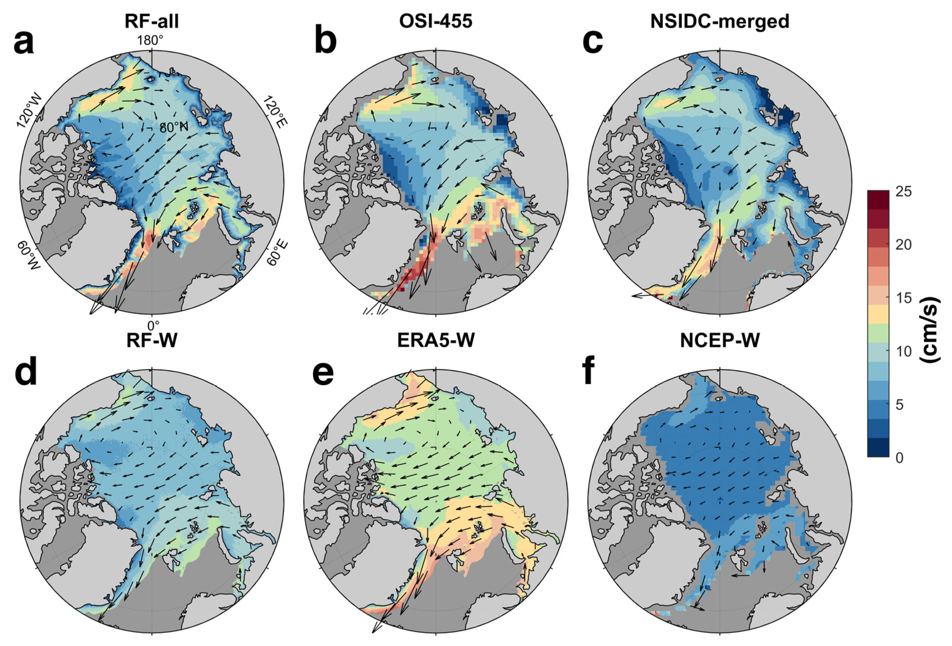
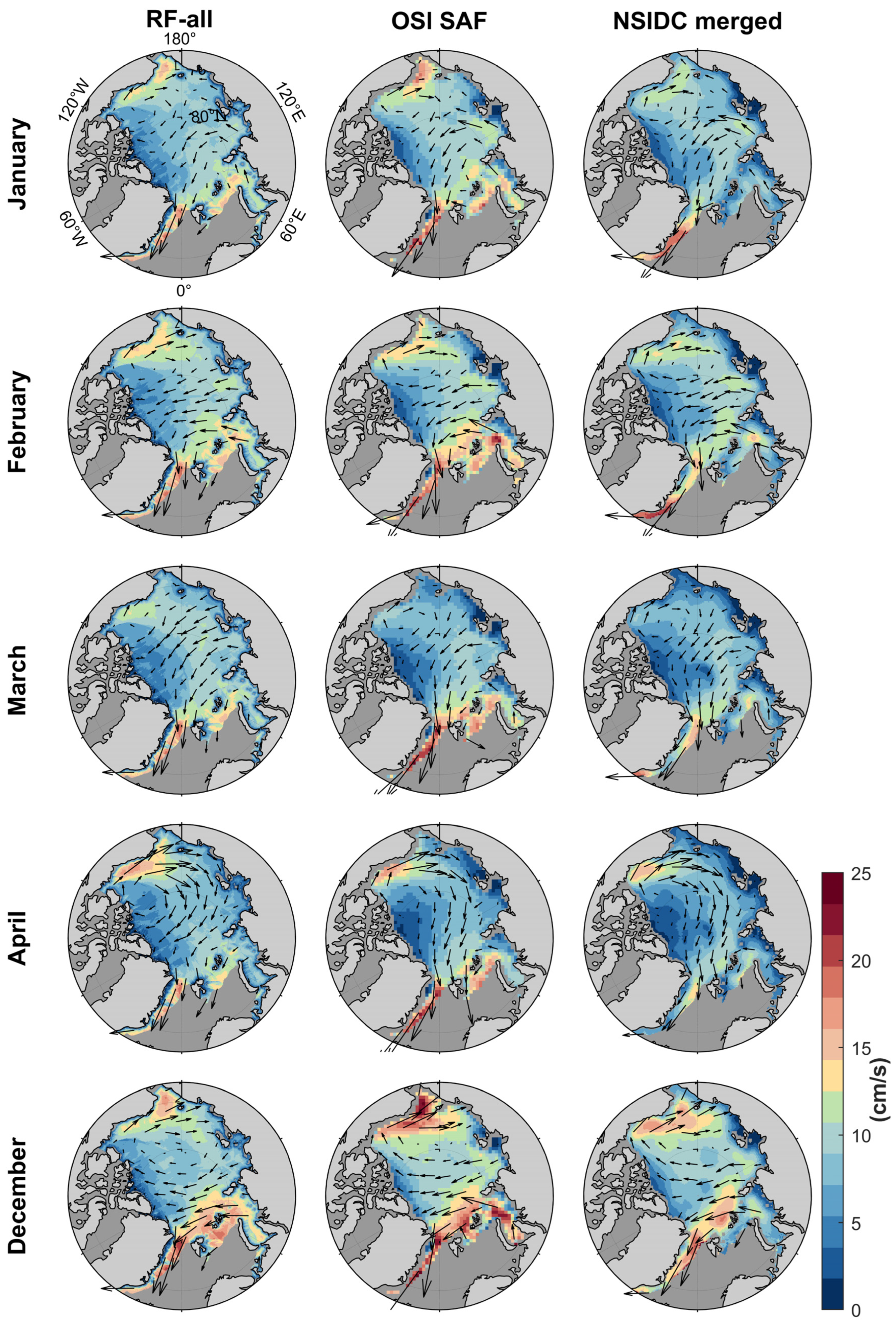
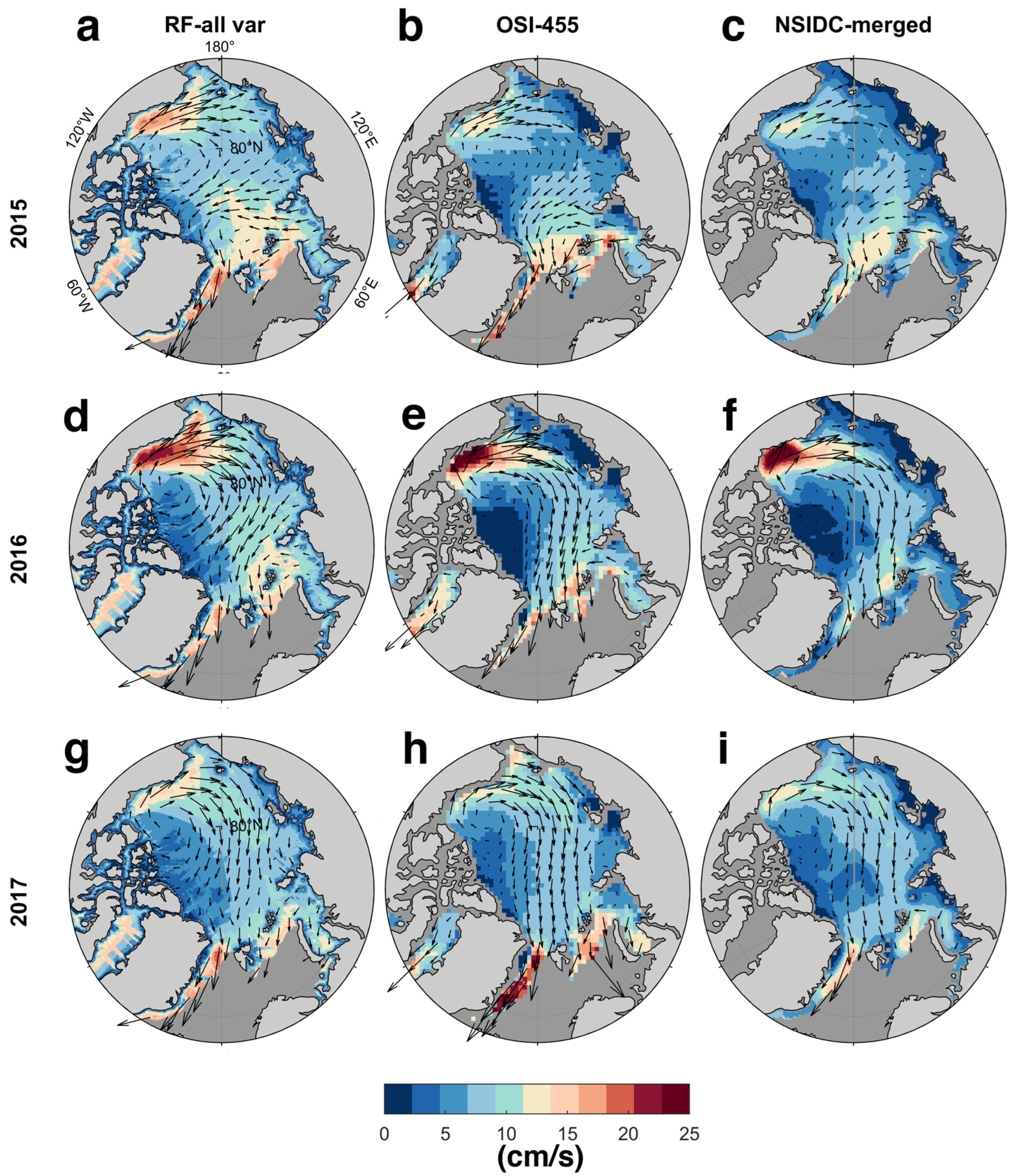
The overall patterns of the 3-year averages in the different datasets are demonstrated in Figure 4; RF-all reached a correlation of 0.9 with the three-year average SIM fields from the OSI-455 and NSIDC-merged data, generally exhibiting a high degree of accordance. Compared with the uniform SIM results obtained by using only the wind field (including RF-W, ERA5-W, and NCEP-W results), RF-all showed a more accurate spatial distribution of SIM as satellite observations. It successfully captured the clockwise circulation in the Beaufort Sea, the Transpolar Drift Stream, and the fast sea ice motion in the Fram Strait. Near the coast, especially in the area north of the CAA, the RF-all results showed a significant decrease in the magnitude of SIM, indicating the coastal resistance to onshore sea ice motion, which was also obvious in the OSI-455 and NSIDC-merged data. The average monthly results are depicted in Figure 5, where the RF-all results align well with those from the OSI-455 and NSIDC data, whether as a three-year average or a monthly average. The RF-all SIM pattern was closer to the OSI-455 data (r = 0.84) than the NSIDC-merged data (r = 0.78) (Table 2), especially in the area around the Svalbard Archipelago and Novaya Zemlya. According to previous studies [26,27,28], OSI-405-c is recognized as a relatively more reliable SIM product than NSIDC. OSI-455 adapted the OSI-405 algorithm’s baseline and shortened the time interval from two days to one day. Hence, our results correlated better with OSI-455, indicating they provided a better look into the real sea ice motion. In terms of the performance of inter-annual variation, a slightly lower correlation with the OSI-455 and NSIDC-merged data occurs in April and March (Table 3). This may be attributed to the transition to spring, when the physical properties of sea ice change and the influence of wind becomes more significant. The main mean bias in the SIM pattern in April was mostly due to the difference in the SIM direction in April 2016 and the magnitude in April 2015, and the rest of the results were in good agreement (Figure A2 and Table A2). Conversely, in December and February, RF-all had the best consistency with those two datasets (above 0.85 and 0.78).
The ice motion results considering only wind (RF-W: Figure 4d, ERA5-W: Figure 4e, and NCEP-W: Figure 4f) presented more homogenous sea ice motion than the other datasets. Generally, ERA5-W with the 2% wind factor rule overestimated the SIM magnitude, while NSIDC-W with a 1% magnitude ratio underestimated it. They were both unable to accurately capture the overall pattern of SIM. Thus, it can be inferred that the RF model is capable of learning ocean current information to a certain extent from SAR data, even when the wind field is the only input variable, since there are strong ocean surface currents that overcome the impact of wind in SIM east of Greenland [2,18,19], where RF-W showed better performance than NCEP-W and ERA5-W.
Furthermore, it is noted that RF-all showed better results in the Beaufort Sea, the north of the CAA and Greenland, and the central Arctic region, while in the East Siberian Sea and the Laptev Sea, it did not perform so well. This indicates that the coastline parameters have a more significant impact on the ice drift influenced by onshore wind, such as in the region to the north of the CAA, while they have less impact in regions influenced by offshore winds, especially in the Laptev Sea. This is reasonable because when sea ice is affected by shoreward winds, the coast will restrict its mobility and change the magnitude and direction of the velocity [3,29].
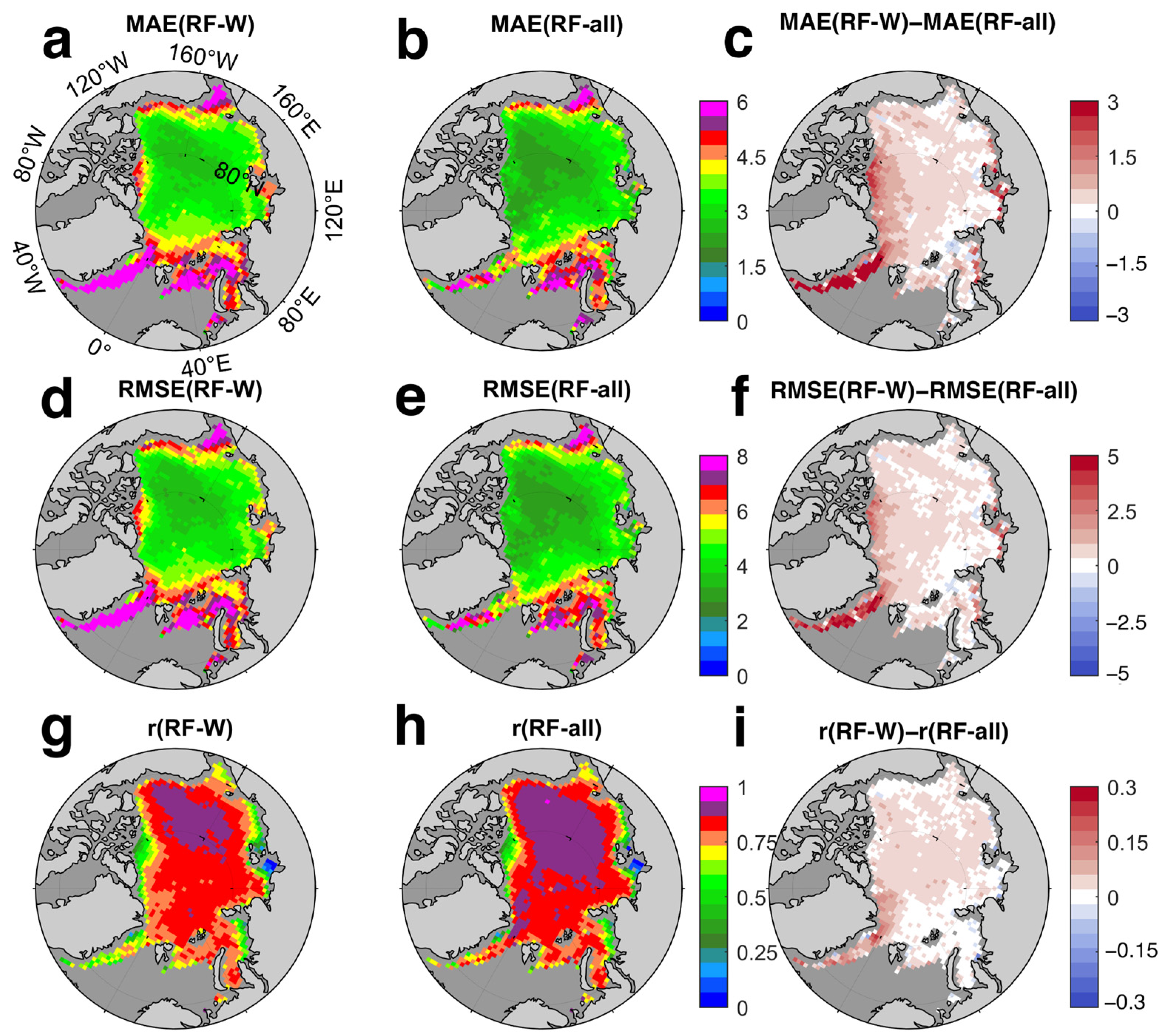
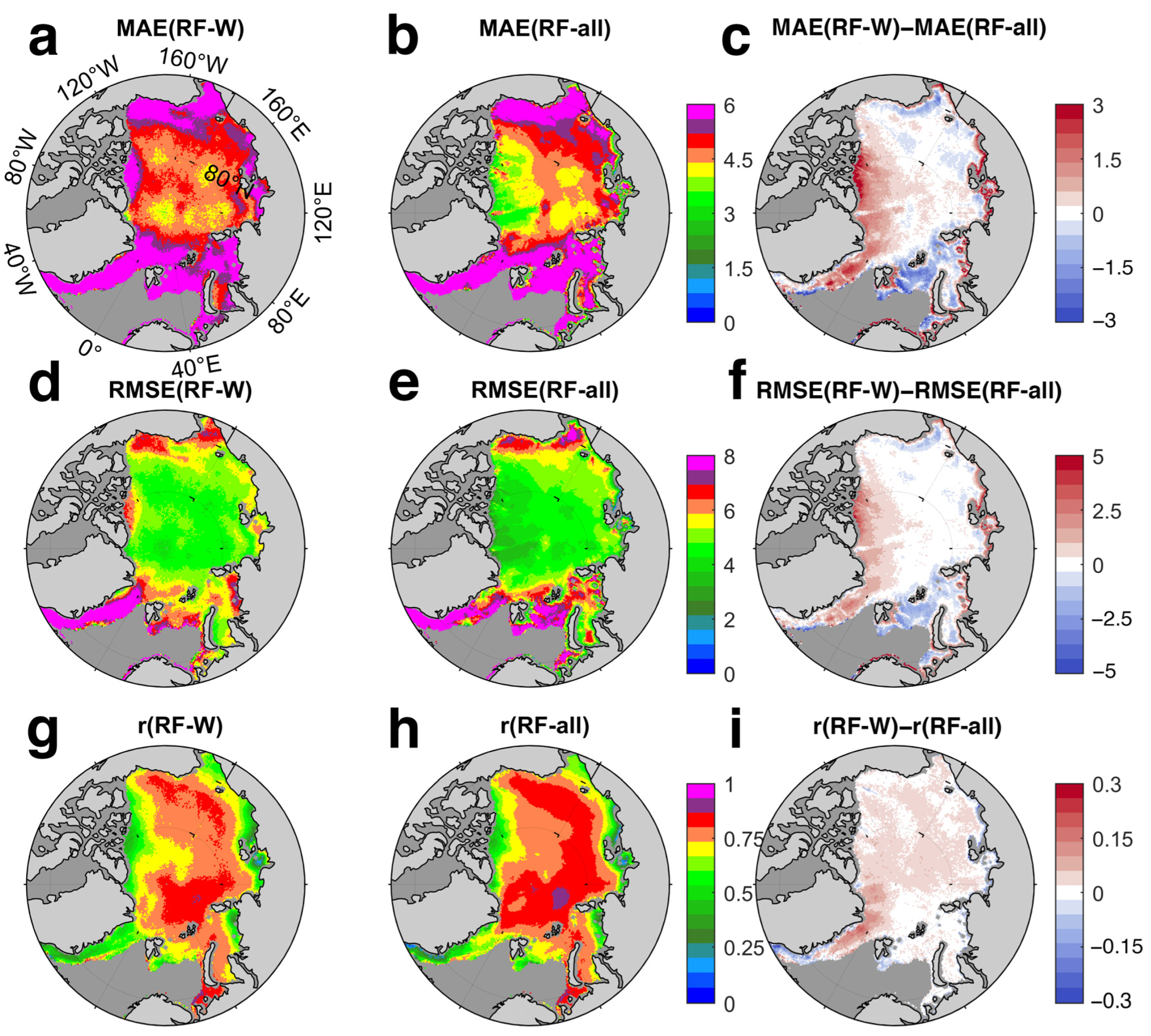
To further analyze the performance of RF-all and RF-W, the spatial distributions of the MAE and RMSE for each scenario using OSI-455 and NSIDC-merged as reference datasets were plotted in Figure 6 and Figure A1, showing more details. It was observed that the MAE and RMSE had similar patterns for RF-all. In the CAA and its surrounding region, as well as in the coastal areas of the Laptev Sea and the Central Arctic, they were relatively small, while in the Chukchi Sea and the Fram Strait, they were relatively large. The overall MAE and RMSE showed great improvements compared with the RF-W, which were particularly strong in the area near Greenland, the Fram Strait, and the north of the CAA. The only exceptions were the Chukchi Sea and the Kara Sea, especially when NSIDC-merged was used as the reference (Figure A1), but in the Chukchi Sea and Kara Sea, the improvements were very small.
Although the performance of RF-all did not precisely align with the two datasets in some small regions, the overall correlations with the OSI-455 and NSIDC-merged datasets were both above 0.78 (see Table 2). The correlation was higher with the OSI-455 data than with the NSIDC-merged data, especially in the Beaufort Sea region and north of the CAA, while low correlations were obvious in the Greenland Sea, where the sea ice motion is influenced by underlying strong southwest East Greenland Current [2,18,19]. In some areas near the shore, e.g., north of Greenland and around the New Siberian Islands, RF-all SIM showed low correlations with OSI-455 and NSIDC-merged. Comparing the correlations of RF-W and RF-all in Figure 6i, the main improvements were located around Greenland, while less significant changes occurred north of the CAA, as depicted by the MAE and RMSE spatial maps.
4.2. Relationship between RF-Derived SIM and Coastline Parameters
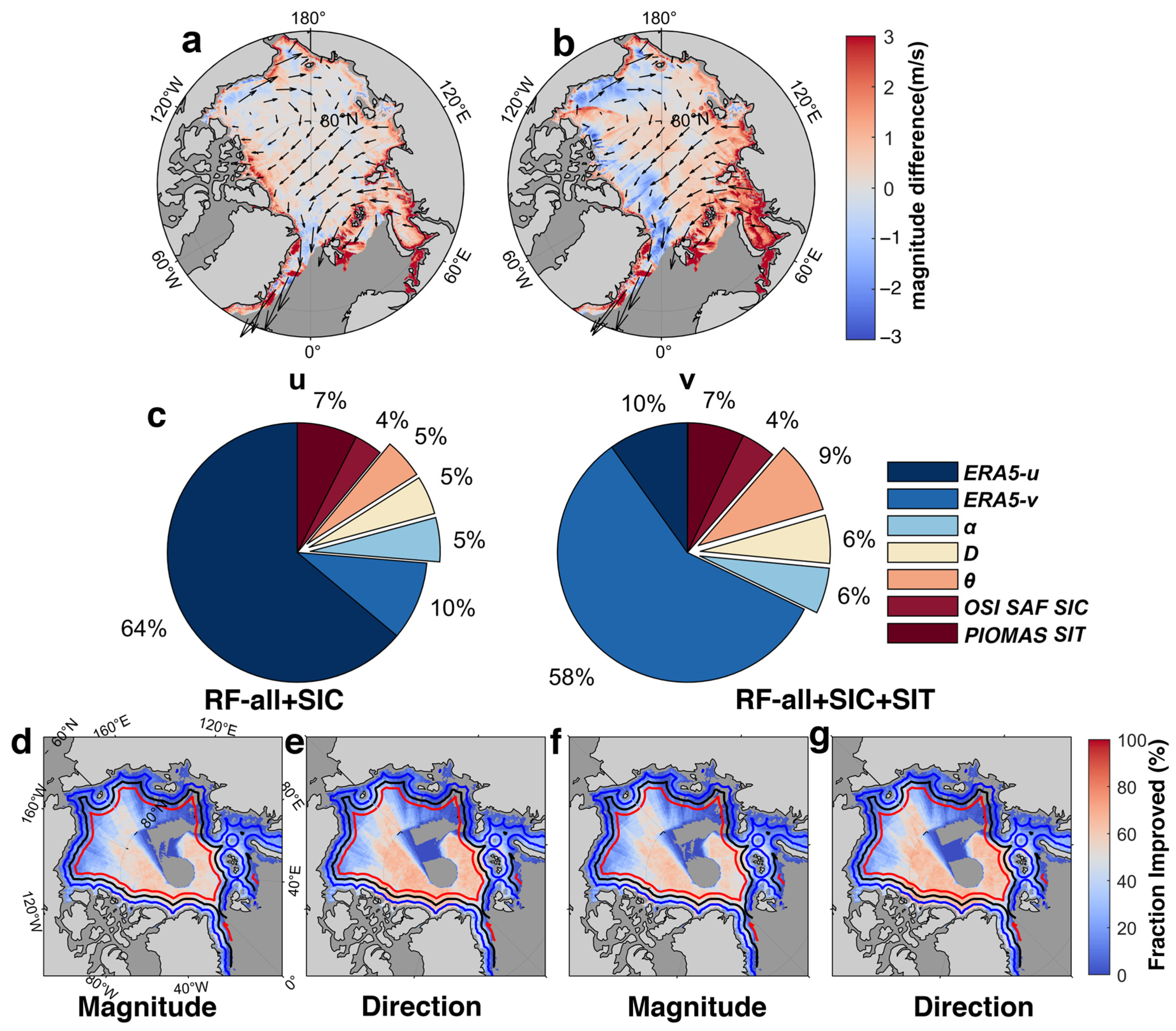
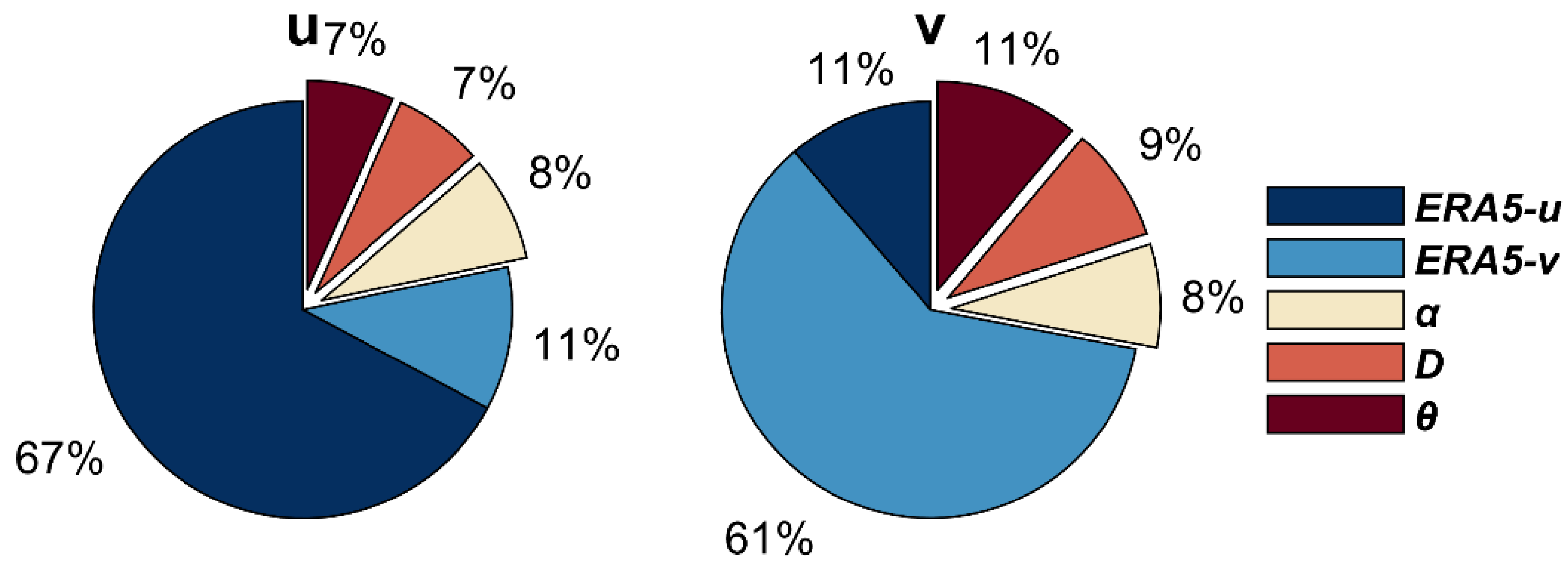
The importance of each predictive variable was calculated using the built-in algorithm of the Python library scikit-learn 1.3.0. As shown in Figure A3, due to the fact that the wind field is a significant factor controlling sea ice motion, the east and west components of the wind vector are the most important variables explaining the corresponding components (u and v) of ice motion. The boundary parameters, accounting for 22% and 28% of the u and v of SIM, respectively, show a relatively uniform distribution among the various parameters. They have an indisputable influence on sea ice motion.
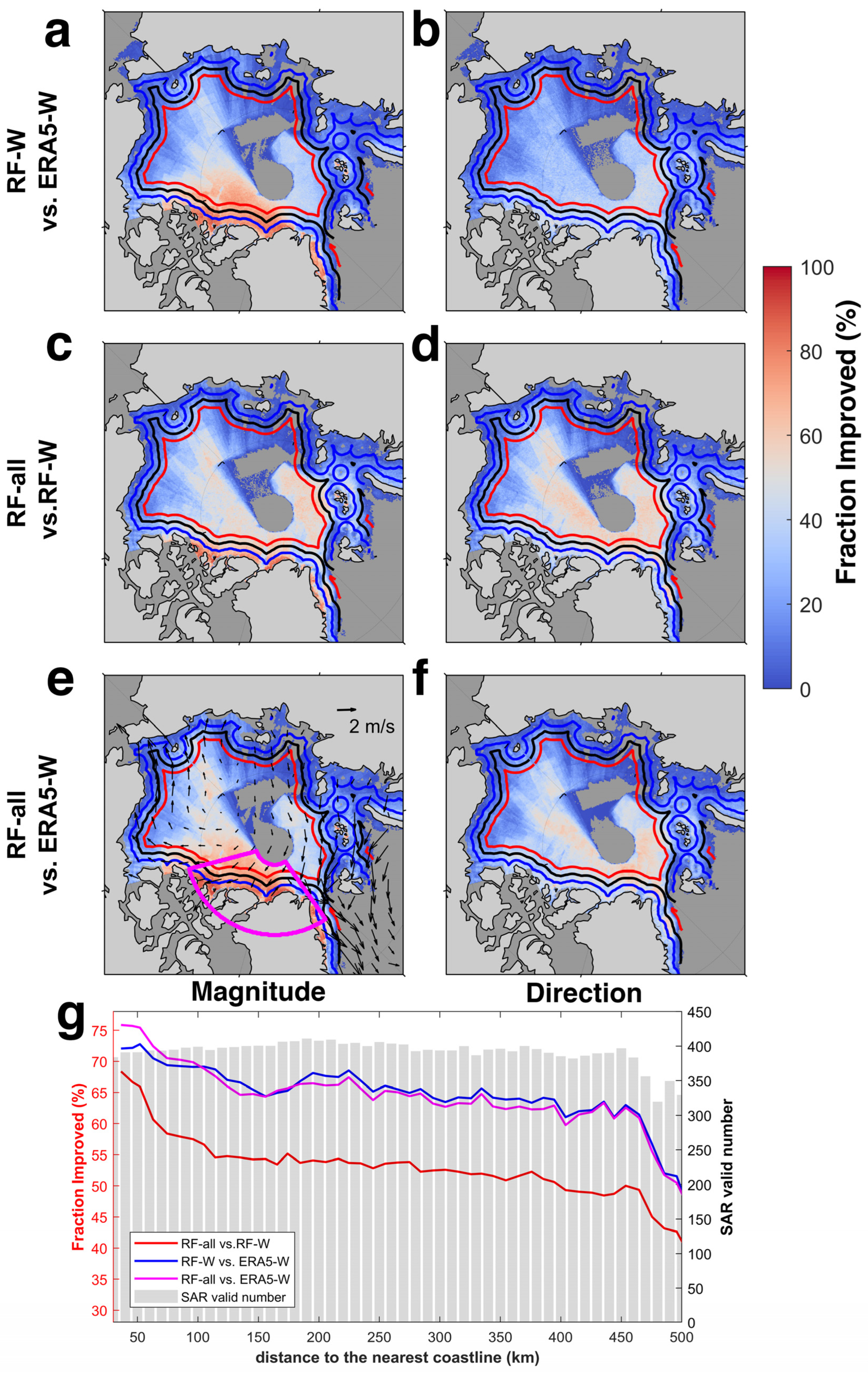
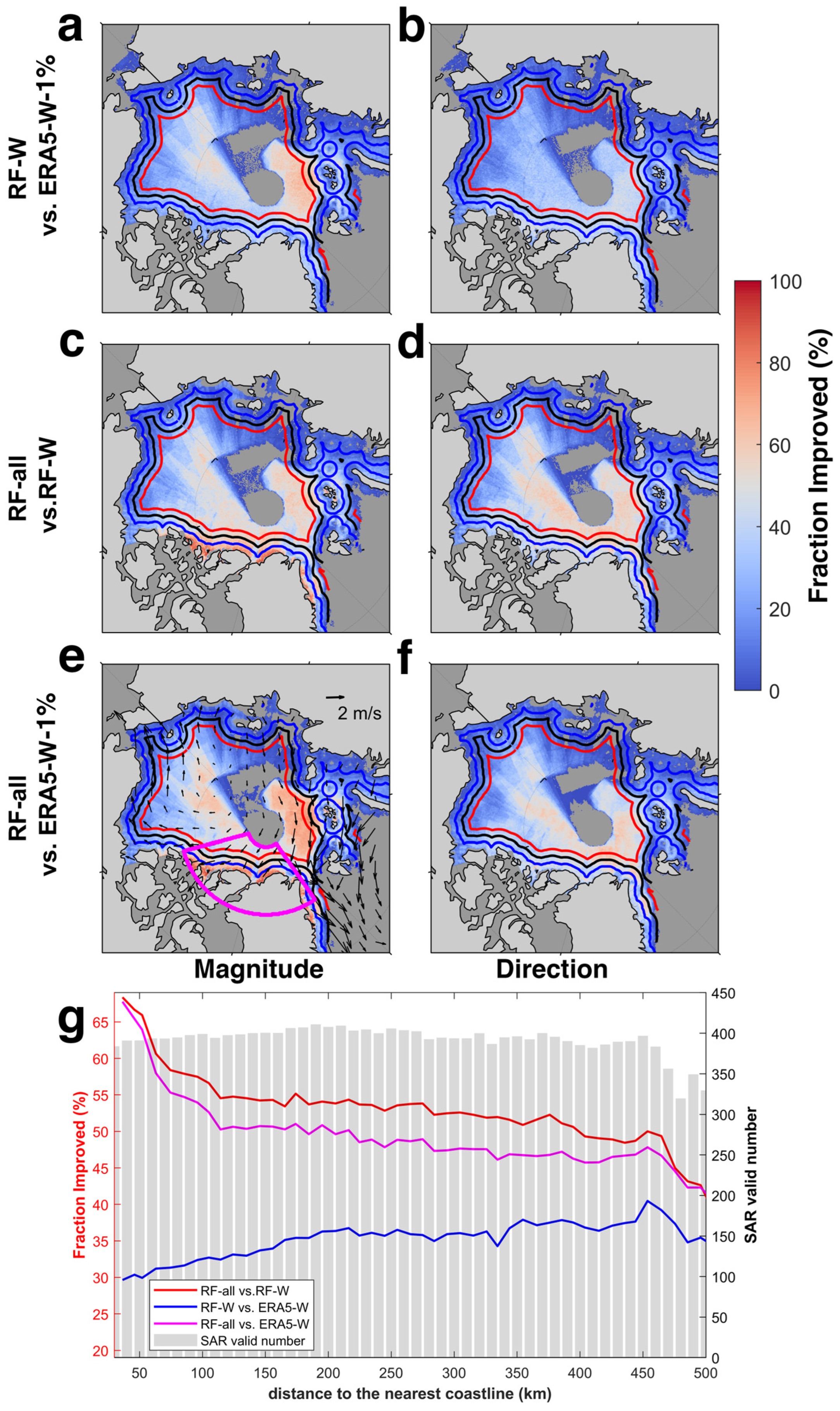
In order to clarify the impact of the coastline parameters on SIM, we converted the u and v of SIM into magnitude and direction and calculated the improvement fraction of the RF-all results compared to the RF-W and ERA5-W results (Figure 7). Here, we followed the same method of improvement fraction as in Palerme and Müller’s research [14]. This fraction was the proportion of the number of grid points that were better (smaller MAE) than the corresponding grid points in the reference data. We used the ice speed field in 2021 because the SAR data (used as reference in this section) from 2018 to 2020 had already been used as training data for our model and there was no public SAR data before 2018.
The results of RF models demonstrated a marked enhancement in the coastal areas north of the CAA and the Central Arctic Ocean, as shown in Figure 7a,c,e. When the SIM was generated based on wind, using random forest improved the results significantly in the area mentioned above compared to the empirical formula results (see Figure 7a). Further enhancement of fractional improvement is seen from Figure 7c when the coastline parameters were taken into account with a primary focus on the regions within 100 km of the coast in the north of the CAA and near the Atlantic side of the Central Arctic Ocean. Overall, RF-all SIM results performed better than ERA5-W results, especially in the north of the CAA and the Central Arctic Ocean (as shown in Figure 7e). In terms of SIM direction, these near-shore improvements were less pronounced, and instead, predominantly in the Central Arctic Ocean and offshore a 200 km zone in the Fram Strait, the SIM was notably improved in RF-all compared with RF-W and ERA5-W results (Figure 7d,f).
Considering the great improvement for SIM magnitude within the area in the north of the CAA (magenta area in Figure 7e), we plotted the line graph below to compare how the magnitude improvement fractions for the different RF model results varied with the distance to the nearest land point. In general, the improvement fraction of RF models gradually decreased as the distance of the sea ice from the coast increased. Among them, both RF-W and RF-all demonstrated similar improvement performances compared to ERA-W in this area (blue and magenta lines in Figure 7g), but RF-all further improved within 100 km of the shore based on RF-W (indicated by the red line). The valid number of SAR data (grey bars in Figure 7g) in this area did not show a rapid change with the distance to the nearest coastline, indicating that the improvement of SIM with distance to coast was unrelated to the uneven distribution of SAR data.
It has been observed that in the north of the CAA, the sea ice is primarily multi-year ice, and the prevailing wind direction is onshore (as indicated by the black vector in Figure 7e). This has resulted in the greatest improvement in terms of fractional coverage, which is consistent with the SIM performance discussed in Section 4.1. Because the coast will restrict the motion of ice when it is impacted by winds blowing towards the shore and the tight packing of sea ice enables the influence of the shore boundary to spread through internal stresses. However, the improvement was very limited in the Chukchi Sea and East Siberian Sea where onshore wind exists. We infer this difference is related to different ice types. In the north of the CAA, thick multi-year ice dominates; the Chukchi Sea and East Siberian Sea, thin first-year ice is predominant. In the literature, the length scale of friction is more for multi-year ice than first-year ice [3,29].
We also considered the NCEP-W results with a 1% wind factor results in the fraction improvement analysis. Since we used ERA5 data when configurating the RF models, we estimated SIM from ERA5 wind data using the same formula, and these SIM data are called ‘ERA5-W-1%’ hereafter (correlation between ERA5-W-1% and NCEP-W was 0.92). The results are shown in Figure A4. In this case, the results for direction were similar with the results for magnitude. For the magnitude compared to ERA5-W-1%, RF-W and RF-all showed more pronounced improvements in the Nansen basin. However, the RF-all results outperformed ERA5-W-1%, especially in the area within 100 km north of the CAA. This also proves the great impact of the coastline parameters in generating SIM, and in the context of sea ice drift estimation, the inclusion of boundary parameters can significantly improve the performance for magnitude but has less impact on direction. The internal ice stress in general tends to align onshore drift into shoreline orientation [29], but here the low improvement could be partly due to the fact that the SIM direction has a high degree of randomness under low speed.
5. Discussion
Sea ice concentration (SIC) and sea ice thickness (SIT) play important roles in sea ice motion estimation or prediction [1,2,3,13,14,15,16]. Here, we also attempted to train the RF model by including SIC and SIT as input variables, to estimate SIM. The daily SIC from OSI SAF OSI-401-d [30] and the SIT from PIOMAS [31] were used in the RF models. In general, including SIC and SIT smoothed the SIM and decreased its differential field.
Our results show that when only the SIC was incorporated, the correlation of SIM and SAR improved from 0.89 to 0.90 compared with SAR. From Figure 8d,e, we infer that the difference between the effect of SIC and the boundary parameters is that inputting SIC in RF models improved the direction more effectively (additionally considering SIT was about the same for both), while the RF model with coastline parameters (RF-all) showed a more significant improvement in SIM magnitude (Figure 7) Furthermore, when considering SIT as an input variable, the correlation of SAR and SIM improved to 0.92. Although the results show that SIC and SIT together accounted for a large proportion of the variable importance (12% and 11% for u and v), when compared with buoy and OSI-455 SIM data (Table A1), the bias, MAE, RMSE, r, and skill, were almost unchanged from those of the RF-all results. According to Figure 8, compared to RF-all, adding SIC and SIT at the same time mainly changed the SIM magnitude in the Kara Sea and Barents Sea, but in general, changes neither in magnitude nor direction are obvious. According to Figure 8c, the overall contribution of SIC and SIT to SIM was lower than that of the shore boundary parameters, and the SIT’s contribution was twice that of the SIC. The improvements in the direction of these two input parameters were slightly larger than in the magnitude, and there is no obvious change near the shore (Figure 8d–g). Considering the limited contribution of SIC and the high uncertainty of the daily SIT derived from the reanalysis system [32], as well as the limited improvement of SIM over the whole Arctic Ocean, we focused on the SIM estimated by the RF model without SIC and SIT inputs.
This article mainly focused on the impact of coastal boundaries on SIM, so the model training relied on SAR data. However, the spatial distribution of the SAR data was uneven, which may impact on the model performance. Our research results show that in RF-all + SIC and RF-all + SIC + SIT results (Figure 8d–g), the regions with significant improvements in SIM basically overlapped with those with abundant SAR data (Figure 1c,d in [14]), while the improvements were more limited in the Eurasian Basin region with less SAR data. In future research, more extensive coverage of Arctic SAR data can be introduced to reduce the impact of the insufficient spatial representation of training data on SIM estimation.
The merging of SIM data from different sources is currently a hot topic in the research and development of SIM products [8,12,33]. The abnormal changes in ice surface characteristics caused by weather processes often lead to a failure of traditional SIM tracking methods. These situations will become more frequent as polar atmospheric river events increase [34,35]. Therefore, the SIM estimated in this study does not depend on the physical characteristics of the sea ice surface and can be used as a reliable SIM data source to integrate with SIM retrieved using satellite imagery, improving the quality of merged SIM products.
6. Conclusions
Machine learning methods are superior in estimating and predicting sea ice motion [13,14,15,16]. However, the existing studies have not fully considered the impact of shore boundaries on the sea ice motion. In this paper, we estimated the daily sea ice motion based on a random forest model, which only depends on surface wind and explicit coastline information. Our results show that the new model could accurately obtain the Arctic sea ice drift fields, and in particular, by considering the coastline information, the correlation with SAR data could be improved from 0.78 to 0.89. The correlations with OSI-455/NSIDC-merged data and buoys were also high (0.78 and 0.75, or higher). Furthermore, this dataset also included the near-shore area within 100–150 km, which fills the gap area near the shore in the existing dataset. The RF-all results showed better results in the areas where SIM is influenced by onshore wind, such as north of the CAA, while the improvement in the region on the Siberian side of the Arctic was not significant. Based on variable importance calculation, the coastline parameters accounted for 22% and 28% of the importance, and after further consideration of sea ice concentration and sea ice thickness, the proportions were 16% and 21% for u and v, respectively.
Previous studies have indicated that, in addition to surface winds, ocean surface currents are also an important factor affecting sea ice motion [18]. Since accurate daily observations of Arctic ocean surface currents are very difficult to obtain, this study did not use them as input variables for the RF models. However, we believe that the coastline parameters themselves limit the movement of ocean surface currents, so the coastline parameters we used also imply information about ocean currents to some extent, and internal friction of sea ice is a major factor in the near-shore zone at onshore wind. This is why introducing coastline parameters can effectively improve ice speed estimation.
It should be noted that, in estimating sea ice motion, since both input variables (wind field and boundary parameters) are relatively easier to obtain than remote sensing or buoy observations, RF shows great potential in operationally retrieving the pan-Arctic sea ice motion.
Author Contributions
Conceptualization, Q.S.; methodology, M.L., J.L. and Q.Y.; software, validation and writing—original draft preparation, L.Z.; formal analysis, L.Z. and Q.Y.; investigation, Q.S., M.L. and J.L.; writing—review and editing, Q.S., M.L., J.L. and Q.Y.; supervision, M.L., J.L. and Q.Y.; project administration, Q.Y.; funding acquisition, Q.Y. and Q.S. All authors have read and agreed to the published version of the manuscript.
Funding
This study was funded by the National Key R&D Program of China (No. 2022YFE0106300), the Southern Marine Science and Engineering Guangdong Laboratory (Zhuhai) (No. SML2023SP217), the National Natural Science Foundation of China (No. 42106220) and the Program of Marine Economy Development Special Fund under Department of Natural Resources of Guangdong Province (No. GDNRC [2022]18).
Data Availability Statement
The Sentinel-1 SAR SIM data used in this study are available from the website: https://resources.marine.copernicus.eu (accessed on 31 January 2024). The ERA5 10 m wind is available at https://cds.climate.copernicus.eu (accessed on 31 January 2024). The IABP buoy SIM data are available at https://www.ncei.noaa.gov/products/international-arctic-buoy-program (accessed on 31 January 2024). The NSIDC Polar Pathfinder Daily 25 km EASE-Grid and OSI SAF 455 SIM data were obtained from https://nsidc.org/data/nsidc-0116/versions/4 (accessed on 31 January 2024) and https://osi-saf.eumetsat.int/products/osi-455 (accessed on 31 January 2024). Further, SIC from OSI SAF OSI-401-d is available from https://osi-saf.eumetsat.int/products/osi-401-d (accessed on 31 January 2024) and PIOMAS SIT can be accessed at https://psc.apl.uw.edu/research/projects/arctic-sea-ice-volume-anomaly/data (accessed on 31 January 2024).
Acknowledgments
We would like to thank four anonymous reviewers for improving the quality of this paper. We also thank Palerme and Müller (2021) [14] for providing Python codes for random forest model publicly, and Mark Tschudi who explained the NSIDC ice velocity consideration in emails.
Conflicts of Interest
The authors declare no conflict of interest.
Appendix A

Table A1.
Evaluation of the performances of the Arctic sea ice drift produced using random forest (RF) algorithms considering sea ice concentration (SIC) and sea ice thickness (SIT) and validation datasets during the period from January 2015 to December 2017(except for May, June, July, August, September, and October). Buoy, OSISAF and NSIDC merged sea ice motion datasets were used as references.
| Bias (cm/s) | MAE (cm/s) | r | RMSE (cm/s) | Skill | |
|---|---|---|---|---|---|
| Reference Dataset: Buoys | |||||
| RF-all + SIC | 0.23 | 3.77 | 0.76 | 4.18 | 0.45 |
| RF-all + SIC + SIT | 0.47 | 3.70 | 0.76 | 4.11 | 0.46 |
| Reference dataset: OSI-455 | |||||
| RF-all + SIC | 0.08 | 3.32 | 0.84 | 3.69 | 0.56 |
| RF-all + SIC + SIT | 0.24 | 3.21 | 0.85 | 3.57 | 0.58 |
| Reference dataset: NSIDC-merged | |||||
| RF-all + SIC | −0.01 | 3.77 | 0.78 | 4.19 | 0.44 |
| RF-all + SIC + SIT | 0.14 | 3.68 | 0.79 | 4.08 | 0.45 |
Table A2.
Correlation (r) in April each year between SIM data.
| r | (RF-All) | (RF-All) | (NSIDC-Merged) |
|---|---|---|---|
| - | - | - | |
| (OSI-455) | (NSIDC-Merged) | (OSI-455) | |
| 2015 | 0.82 | 0.76 | 0.72 |
| 2016 | 0.82 | 0.78 | 0.79 |
| 2017 | 0.84 | 0.80 | 0.75 |
Figure A1.
Same as Figure 6, but NSIDC-merged was used as reference.
Figure A1.
Same as Figure 6, but NSIDC-merged was used as reference.

Figure A2.
The April averages in 2015, 2016, and 2017 of sea ice drift magnitude (shading) and velocity (vectors) for RF-all (a,d,g), OSI-455 (b,e,h), and NSIDC-merged (c,f,i).
Figure A2.
The April averages in 2015, 2016, and 2017 of sea ice drift magnitude (shading) and velocity (vectors) for RF-all (a,d,g), OSI-455 (b,e,h), and NSIDC-merged (c,f,i).

Figure A3.
Pie chart of the variable importance of each input parameter of RF all var result for u and v components.
Figure A3.
Pie chart of the variable importance of each input parameter of RF all var result for u and v components.

Figure A4.
Same as Figure 7, but for ERA5-W-1% instead of EAR5-W.
Figure A4.
Same as Figure 7, but for ERA5-W-1% instead of EAR5-W.

References
- Coon, M.D. A Review of AIDJEX Modeling. Sea Ice Process. Models 1980, 12, 25. [Google Scholar] [CrossRef]
- Hibler, W.D. A Dynamic Thermodynamic Sea Ice Model. J. Phys. Ocean. 1979, 9, 815–846. [Google Scholar] [CrossRef]
- Leppäranta, M. The Drift of Sea Ice; Springer Science & Business Media: Berlin/Heidelberg, Germany, 2011; ISBN 3642046835. [Google Scholar]
- Watkins, D.M.; Bliss, A.C.; Hutchings, J.K.; Wilhelmus, M.M. Evidence of Abrupt Transitions Between Sea Ice Dynamical Regimes in the East Greenland Marginal Ice Zone. Geophys. Res. Lett. 2023, 50, e2023GL103558. [Google Scholar] [CrossRef]
- Zhao, Y.; Liu, A.K. Arctic sea-ice motion and its relation to pressure field. J. Oceanogr. 2007, 63, 505–515. [Google Scholar] [CrossRef]
- Lavergne, T.; Eastwood, S.; Teffah, Z.; Schyberg, H.; Breivik, L. Sea Ice Motion from Low-resolution Satellite Sensors: An Alternative Method and Its Validation in the Arctic. J. Geophys. Res. Ocean. 2010, 115, C10. [Google Scholar] [CrossRef]
- Ezraty, R.; Girard-Ardhuin, F.; Piollé, J.-F.; Kaleschke, L.; Heygster, G. Arctic and Antarctic Sea Ice Concentration and Arctic Sea Ice Drift Estimated from Special Sensor Microwave Data; Département d’Océanographie Physique et Spatiale, IFREMER; University of Bremen Germany: Bremen, Germany, 2007; Volume 2. [Google Scholar]
- Tschudi, M.A.; Meier, W.N.; Scott Stewart, J. An Enhancement to Sea Ice Motion and Age Products at the National Snow and Ice Data Center (NSIDC). Cryosphere 2020, 14, 1519–1536. [Google Scholar] [CrossRef]
- Karvonen, J. Operational SAR-Based Sea Ice Drift Monitoring over the Baltic Sea. Ocean. Sci. 2012, 8, 473–483. [Google Scholar] [CrossRef]
- Frost, A.; Jacobsen, S.; Singha, S. High Resolution Sea Ice Drift Estimation Using Combined TerraSAR-X and RADARSAT-2 Data: First Tests. In Proceedings of the 2017 IEEE International Geoscience and Remote Sensing Symposium (IGARSS), Fort Worth, TX, USA, 23–28 July 2017; pp. 342–345. [Google Scholar]
- Howell, S.E.L.; Brady, M.; Komarov, A.S. Generating Large-Scale Sea Ice Motion from Sentinel-1 and the RADARSAT Constellation Mission Using the Environment and Climate Change Canada Automated Sea Ice Tracking System. Cryosphere 2022, 16, 1125–1139. [Google Scholar] [CrossRef]
- Lavergne, T.; Down, E. Product User’s Manual for the Global Sea Ice Drift Climate Data Record v1. Available online: https://osisaf-hl.met.no/sites/osisaf-hl/files/user_manuals/osisaf_cdop3_ss2_pum_sea-ice-drift-lr-cdr_v1p0.pdf (accessed on 31 January 2024).
- Petrou, Z.I.; Tian, Y. Prediction of Sea Ice Motion with Convolutional Long Short-Term Memory Networks. IEEE Trans. Geosci. Remote Sens. 2019, 57, 6865–6876. [Google Scholar] [CrossRef]
- Palerme, C.; Müller, M. Calibration of Sea Ice Drift Forecasts Using Random Forest Algorithms. Cryosphere 2021, 15, 3989–4004. [Google Scholar] [CrossRef]
- Zhai, J.; Bitz, C.M. A Machine Learning Model of Arctic Sea Ice Motions. arXiv 2021, arXiv:2108.10925. [Google Scholar]
- Hoffman, L.; Mazloff, M.R.; Gille, S.T.; Giglio, D.; Bitz, C.M.; Heimbach, P.; Matsuyoshi, K. Machine Learning for Daily Forecasts of Arctic Sea Ice Motion: An Attribution Assessment of Model Predictive Skill. Artif. Intell. Earth Syst. 2023, 2, 230004. [Google Scholar] [CrossRef]
- Strobl, C.; Boulesteix, A.-L.; Zeileis, A.; Hothorn, T. Bias in Random Forest Variable Importance Measures: Illustrations, Sources and a Solution. BMC Bioinform. 2007, 8, 25. [Google Scholar] [CrossRef] [PubMed]
- Thorndike, A.S.; Colony, R. Sea Ice Motion in Response to Geostrophic Winds. J. Geophys. Res. Ocean. 1982, 87, 5845–5852. [Google Scholar] [CrossRef]
- Kimura, N.; Wakatsuchi, M. Relationship between Sea-ice Motion and Geostrophic Wind in the Northern Hemisphere. Geophys. Res. Lett. 2000, 27, 3735–3738. [Google Scholar] [CrossRef]
- Maeda, K.; Kimura, N.; Yamaguchi, H. Temporal and Spatial Change in the Relationship between Sea-Ice Motion and Wind in the Arctic. Polar Res. 2020, 39. [Google Scholar] [CrossRef]
- Hersbach, H.; Bell, B.; Berrisford, P.; Hirahara, S.; Horányi, A.; Muñoz-Sabater, J.; Nicolas, J.; Peubey, C.; Radu, R.; Schepers, D. The ERA5 Global Reanalysis. Q. J. R. Meteorol. Soc. 2020, 146, 1999–2049. [Google Scholar] [CrossRef]
- Sakov, P.; Counillon, F.; Bertino, L.; Lisæter, K.A.; Oke, P.R.; Korablev, A. TOPAZ4: An Ocean-Sea Ice Data Assimilation System for the North Atlantic and Arctic. Ocean. Sci. 2012, 8, 633–656. [Google Scholar] [CrossRef]
- Breiman, L. Random Forests. Mach. Learn. 2001, 45, 5–32. [Google Scholar] [CrossRef]
- Pedregosa, F.; Varoquaux, G.; Gramfort, A.; Michel, V.; Thirion, B.; Grisel, O.; Blondel, M.; Prettenhofer, P.; Weiss, R.; Dubourg, V. Scikit-Learn: Machine Learning in Python. J. Mach. Learn. Res. 2011, 12, 2825–2830. [Google Scholar]
- Thomson, R.E.; Emery, W.J. Data Analysis Methods in Physical Oceanography; Newnes: Boston, MA, USA, 2014; ISBN 0123877830. [Google Scholar]
- Sumata, H.; Lavergne, T.; Girard-Ardhuin, F.; Kimura, N.; Tschudi, M.A.; Kauker, F.; Karcher, M.; Gerdes, R. An Intercomparison of Arctic Ice Drift Products to Deduce Uncertainty Estimates. J. Geophys. Res. Ocean. 2014, 119, 4887–4921. [Google Scholar] [CrossRef]
- Hwang, B. Inter-Comparison of Satellite Sea Ice Motion with Drifting Buoy Data. Int. J. Remote Sens. 2013, 34, 8741–8763. [Google Scholar] [CrossRef]
- Wang, X.; Chen, R.; Li, C.; Chen, Z.; Hui, F.; Cheng, X. An Intercomparison of Satellite Derived Arctic Sea Ice Motion Products. Remote Sens. 2022, 14, 1261. [Google Scholar] [CrossRef]
- Leppäranta, M.; Hibler, W.D., III. The role of plastic ice interaction in marginal ice zone dynamics. J. Geophys. Res. Ocean. 1985, 90, 11899–11909. [Google Scholar] [CrossRef]
- Baordo, F.; Vargas, L.F.; Howe, E. OSI SAF Product User Manual for Global Sea Ice Concentration Level 2 and Level 3, OSI-410-a, OSI-401-d, OSI-408-a. Version 1.2, 14/6/2023. Available online: https://osisaf-hl.met.no/sites/osisaf-hl/files/user_manuals/osisaf_pum_ice-conc_l2-3_v1p2.pdf (accessed on 9 October 2023).
- Zhang, J.; Rothrock, D.A. Modeling Global Sea Ice with a Thickness and Enthalpy Distribution Model in Generalized Curvilinear Coordinates. Mon. Weather. Rev. 2003, 131, 845–861. [Google Scholar] [CrossRef]
- Schweiger, A.; Lindsay, R.; Zhang, J.; Steele, M.; Stern, H.; Kwok, R. Uncertainty in Modeled Arctic Sea Ice Volume. J. Geophys. Res. Ocean. 2011, 116, C8. [Google Scholar] [CrossRef]
- Fang, Y.; Wang, X.; Chen, Z. Arctic daily 1 km sea ice drift product: 2018–2020, version 1.0[DS/OL]. V1. Science Data Bank 2023. Available online: https://www.scidb.cn/en/detail?dataSetId=8cf81c7a69004c2ebc94b12ddbb7ae72 (accessed on 31 January 2024).
- Liang, K.; Wang, J.; Luo, H.; Yang, Q. The Role of Atmospheric Rivers in Antarctic Sea Ice Variations. Geophys. Res. Lett. 2023, 50, e2022GL102588. [Google Scholar] [CrossRef]
- Zhang, P.; Chen, G.; Ting, M.; Ruby, L.L.; Guan, B.; Li, L. More frequent atmospheric rivers slow the seasonal recovery of Arctic sea ice. Nat. Clim. Chang. 2023, 13, 266–273. [Google Scholar] [CrossRef]
Figure 1.
(a) Schematic diagram of the relationship between a drift ice parcel in the circle center and the near-shore boundary, showing distance (D) and azimuth angle (α) to the nearest coastline, and the distance between the farthest and closest points (D’), and sector angle (θ) of the influencing coastline. (b) Flow chart of the sea ice motion estimation based on random forest model.

Figure 2.
Mean absolute error (MAE) (cm/s) of the random forest models depending on (a) max features and (b) the number of decision trees. Daily Synthetic Aperture Radar (SAR) observations were used as reference.
Figure 2.
Mean absolute error (MAE) (cm/s) of the random forest models depending on (a) max features and (b) the number of decision trees. Daily Synthetic Aperture Radar (SAR) observations were used as reference.

Figure 3.
(a) Mean absolute error (MAE) (blue) and root mean squared error (RMSE) (red). (b) Correlation (r) of SIM with respect to daily SAR observations.
Figure 3.
(a) Mean absolute error (MAE) (blue) and root mean squared error (RMSE) (red). (b) Correlation (r) of SIM with respect to daily SAR observations.

Figure 4.
The 2015–2017 averages of sea ice drift magnitude (shading) and velocity (vectors) for (a) RF-all, (b) OSI-455, (c) NSIDC-merged, (d) RF-W, (e) ERA5-W, and (f) NCEP-W.
Figure 4.
The 2015–2017 averages of sea ice drift magnitude (shading) and velocity (vectors) for (a) RF-all, (b) OSI-455, (c) NSIDC-merged, (d) RF-W, (e) ERA5-W, and (f) NCEP-W.

Figure 5.
The 2015–2017 monthly averages of sea ice drift magnitude (shading) and velocity (vectors) for RF-all (first column), OSI-455 (second column), and NSIDC-merged (third column).
Figure 5.
The 2015–2017 monthly averages of sea ice drift magnitude (shading) and velocity (vectors) for RF-all (first column), OSI-455 (second column), and NSIDC-merged (third column).

Figure 6.
During the winter from 2015 to 2017, mean absolute error (MAE) of (a) RF-W and (b) RF-all and (c) their difference (MAE(RF-W)–MAE(RF-all)), (d–f) show root mean squared error (RMSE), and (g–i) show correlation. OSI-455 was used as reference.
Figure 6.
During the winter from 2015 to 2017, mean absolute error (MAE) of (a) RF-W and (b) RF-all and (c) their difference (MAE(RF-W)–MAE(RF-all)), (d–f) show root mean squared error (RMSE), and (g–i) show correlation. OSI-455 was used as reference.

Figure 7.
Improvement fraction () of SIM based on the MAE in the year of 2021 (December–April) for (a,b) RF-W outperforms ERA5-W, (c,d) RF-all outperforms RF-W, and (e,f) RF-all outperform ERA5-W for SIM magnitude (first column) and direction (second column). Daily SAR observations have been used as reference. The blue, black, and red outline represents offshore distances of 100 km, 200 km, and 300 km, respectively. (g) Relation between magnitude improvement fraction (lines), valid SAR data number (grey bars), and distance to the nearest land point within the magenta area in (e), respectively.

Figure 8.
The 2015–2017 monthly averages of sea ice drift speed (shading) and velocity (vectors) for (a) magnitude of difference of considering SIC minus RF-all var and velocity of considering SIC. (b) Same as (a) but for considering SIC and SIT. (c) Pie charts of the variable importance of each input parameter of RF all var considering SIC and SIT. (d,e) Fraction of Arctic SIM estimated by the RF models considering SIC which outperform RF-all. (f,g) Same as (d,e) but for considering SIC and SIT. Daily SAR observations were used as reference. The blue, black, and red outlines represent offshore distances of 100 km, 200 km, and 300 km, respectively.

Table 1.
Variables and configurations of different RF SIM models used in this work.
| Input Variable | Target Variable | ||||||
|---|---|---|---|---|---|---|---|
| ERA5 10 m Wind (W) | Distance (D) | Azimuth Angle (α) | Sector Angle of Coastline Based on a Maximum Extend of 90 km (θ90 km) | OSI SAF OSI-401-d Ice Concentration (SIC) | PIOMAS Sea Ice Thickness (SIT) | SAR SIM | |
| RF-W | √ * | √ | |||||
| RF-all | √ | √ | √ | √ | √ | ||
| RF-all + SIC | √ | √ | √ | √ | √ | ||
| RF-all + SIC + SIT | √ | √ | √ | √ | √ | √ | √ |
* √ represents that the variable is included.
Table 2.
Evaluation of the performances of the Arctic sea ice drift produced using random forest (RF) algorithms and validation datasets during the period from January 2015 to December 2017 (except for May, June, July, August, September, October, and November). Buoy, OSI SAF, and NSIDC merged sea ice motion datasets were used as references.
| Bias (cm/s) | MAE (cm/s) | r | RMSE (cm/s) | Skill | |
|---|---|---|---|---|---|
| Reference Dataset: Buoys | |||||
| RF-all | 0.23 | 3.83 | 0.75 | 4.26 | 0.45 |
| RF-W | 0.12 | 4.95 | 0.57 | 5.50 | 0.39 |
| ERA5-W | 0.04 | 5.87 | 0.58 | 6.52 | 0.28 |
| NCEP-W | 0.44 | 5.26 | 0.79 | 7.51 | 0.19 |
| OSI-455 | −0.04 | 3.71 | 0.74 | 5.33 | 0.42 |
| NSIDC-merged | −0.04 | 1.26 | 0.97 | 1.98 | 0.79 |
| Reference dataset: OSI-455 | |||||
| RF-all | 0.13 | 3.31 | 0.84 | 3.68 | 0.56 |
| RF-W | 0.10 | 3.87 | 0.77 | 4.30 | 0.49 |
| ERA5-W | 0.39 | 4.93 | 0.78 | 6.27 | 0.28 |
| NCEP-W | 0.91 | 5.00 | 0.75 | 6.63 | 0.24 |
| Reference dataset: NSIDC merged | |||||
| RF-all | −0.01 | 3.91 | 0.78 | 5.07 | 0.31 |
| RF-W | 0.02 | 3.99 | 0.72 | 4.43 | 0.39 |
| ERA5-W | −0.11 | 5.27 | 0.70 | 5.84 | 0.18 |
| NCEP-W | 0.54 | 3.59 | 0.79 | 4.81 | 0.33 |
Table 3.
Monthly correlation (r) between SIM data.
| r | (RF-All) - (OSI-455) | (RF-All) - (NSIDC-Merged) | (NSIDC-Merged) - (OSI-455) |
|---|---|---|---|
| January | 0.83 | 0.75 | 0.68 |
| February | 0.85 | 0.78 | 0.73 |
| March | 0.82 | 0.74 | 0.70 |
| April | 0.82 | 0.75 | 0.71 |
| December | 0.86 | 0.80 | 0.76 |
| all | 0.84 | 0.78 | 0.75 |
Disclaimer/Publisher’s Note: The statements, opinions and data contained in all publications are solely those of the individual author(s) and contributor(s) and not of MDPI and/or the editor(s). MDPI and/or the editor(s) disclaim responsibility for any injury to people or property resulting from any ideas, methods, instructions or products referred to in the content. |
© 2024 by the authors. Licensee MDPI, Basel, Switzerland. This article is an open access article distributed under the terms and conditions of the Creative Commons Attribution (CC BY) license (https://creativecommons.org/licenses/by/4.0/).
Share and Cite
MDPI and ACS Style
Zhang, L.; Shi, Q.; Leppäranta, M.; Liu, J.; Yang, Q. Estimating Winter Arctic Sea Ice Motion Based on Random Forest Models. Remote Sens. 2024, 16, 581. https://doi.org/10.3390/rs16030581
AMA Style
Zhang L, Shi Q, Leppäranta M, Liu J, Yang Q. Estimating Winter Arctic Sea Ice Motion Based on Random Forest Models. Remote Sensing. 2024; 16(3):581. https://doi.org/10.3390/rs16030581
Chicago/Turabian StyleZhang, Linxin, Qian Shi, Matti Leppäranta, Jiping Liu, and Qinghua Yang. 2024. "Estimating Winter Arctic Sea Ice Motion Based on Random Forest Models" Remote Sensing 16, no. 3: 581. https://doi.org/10.3390/rs16030581
Note that from the first issue of 2016, this journal uses article numbers instead of page numbers. See further details here.