

Geolocalization from Aerial Sensing Images Using Road Network Alignment

1
Xi’an Research Institute of Hi-Tech, Xi’an 710025, China
2
Rearch Institute for Mathematics and Mathematical Technology, Xi’an Jiaotong University, Xi’an 710049, China
*
Author to whom correspondence should be addressed.
Remote Sens. 2024, 16(3), 482; https://doi.org/10.3390/rs16030482
Submission received: 13 November 2023
/
Revised: 18 January 2024
/
Accepted: 20 January 2024
/
Published: 26 January 2024
(This article belongs to the Special Issue Advanced Methods for Motion Estimation in Remote Sensing)
Abstract
:Estimating the geographic positions in GPS-denied environments is of great significance to the safe flight of unmanned aerial vehicles (UAVs). In this paper, we propose a novel geographic position estimation method for UAVs after road network alignment. We discuss the generally overlooked issue, namely, how to estimate the geographic position of the UAV after successful road network alignment, and propose a precise robust solution. In our method, the optimal initial solution of the geographic position of the UAV is first estimated from the road network alignment result, which is typically presented as a homography transformation between the observed road map and the reference one. The geographic position estimation is then modeled as an optimization problem to align the observed road with the reference one to improve the estimation accuracy further. Experiments on synthetic and real flight aerial image datasets show that the proposed algorithm can estimate more accurate geographic position of the UAV in real time and is robust to the errors from homography transformation estimation compared to the currently commonly-used method.
1. Introduction
Estimating the geographic position is a fundamental requirement for UAVs, which is usually achieved using GPS [1]. However, there also exist some situations where the GPS is unreliable, such as when the GPS is jammed. Since ample, free, and georeferenced maps, which cover many parts of the globe, are available online, such as the satellite imagery from Google Maps or the road map for OpenStreetMap (OSM), many researchers have tried to utilize georeferenced maps to solve the geolocalization problem for UAVs in GPS-denied environments.
Such methods model geolocalization using a georeferenced map as an image registration problem where the core issue is to estimate the transformation that aligns the observed aerial image from the onboard camera to a known georeferenced map. The transformation is often modeled as a similarity transformation when the optical axis of the camera is perpendicular to the ground or more generally as a homography transformation. Many researchers have tried to meet the challenge of the image registration problem using robust low-level vision features [2,3,4,5] or semantic vision features [6,7,8]. Generally speaking, geolocalization using georeferenced maps can be divided into two categories: geolocalization using original satellite imagery and geolocalization using semantic maps, such as a road map or building contour.
Geolocalization using satellite imagery: Geolocalization using satellite imagery is more intuitive. To get around the difficulties in image registration caused by the significant difference between the observed aerial images and satellite imagery, early attempts usually utilize robust low-level vision features to perform image registration. In [2,3], the crosscorrelation and the HOG were used to measure the similarity between two images to estimate a 2D translation between two rotation-and-scale-aligned images. Ref. [4] used mutual information as the similarity metric and utilized the template matching method to estimate the similarity transformation. Recently, some researchers have tried to solve the satellite imagery registration problem with deep learning-based methods. Ref. [5] followed the idea proposed in [9] and registered aerial images to satellite imagery by aligning a feature map learned with a VGG16 network [10], and they reported a localization accuracy of 8 m. Ref. [11] proposed a localization solution using the Monte Carlo localization method, where the similarity between the onboard aerial image and the reference satellite imageries was measured using a convolutional neural network. Ref. [12] estimated the geographic position of UAVs by aligning onboard aerial images to satellite imagery using SuperPoint [13], which is a kind of local descriptor.
Geolocalization using semantic maps: Benefitting from the high stability and reliability of semantic maps and the improved performance of semantic segmentation using deep learning techniques [14,15,16], geolocalization using semantic maps has attracted the attention of more researchers. In [6], building contours were employed to match to semantic maps using the Hu moments [17] approach with a carefully designed pipeline. In [7,8], road intersections were utilized to build the feature correspondences between an aerial image and a reference road map to reduce the error accumulation caused by inertial navigation. In [18], a large-area road geolocalization method was proposed, where the geometric hashing method was utilized to align the road fragment obtained by car tracking to a known road map. Different from the aforementioned methods, which use a similarity transformation hypothesis and thus only work when the camera is nadir, in our prior work [19,20], we proposed two projective-invariant geometric features and the accompanying matching methods and achieved road network alignment for aerial images with projective perspectives over a sizable search region. In contrast to these two-stage methods, where semantic segmentation and shape matching are separated, Ref. [21] proposed to regress the similarity transformation between an aerial image and its reference road map using a Siamese network. Their approach, however, is only useful at locations with complex-shaped roadways, such as highway intersections.
Camera pose estimation: Even though matching to georeference maps is studied in many literature works, the subsequent issue, accurate geographic position estimation, is often disregarded. Camera pose estimation is a classical problem in multiple-view geometry and also a fundamental task in many computer vision applications. The problem is well solved in the case of estimating the camera pose between two central projection images. The problem can be solved using the algorithms proposed in [22] or [23] when the scenario is assumed to be planar. More generally, Refs. [24,25] proposed methods to recover the camera motion from the fundamental matrix between two frames without the planar assumption. In addition, the camera pose can be estimated from correspondences between 2D image points and 3D object points when the depth of the scene is known using the methods in [26,27], which details the perspective-n-point (PnP) problem. However, there is still no public research paper which addresses the problem of estimating the camera motion between a central projection image and an orthographic projection image, which is the case when we need to recover the geographic position of the camera by matching it to a georeferenced orthographic map.
Some works on geolocalization use the translation of the estimated similarity transformation to recover the geographic position of the camera [2,3,4,21], which is equal to computing the projection point of the image center using the estimated transformation. Such methods only work properly when the optical axis of the camera is perpendicular to the ground, or external information is used to compensate for the deviation [12]. Some other works [18,19,20] donated the geolocalization result using the homography or simplified similarity transformation between the aerial image and the georeferenced map, wherein the geographic position of the UAV was thus unavailable. To the best of our knowledge, no public research article has addressed the problem of estimating the geographic position of the camera when the transformation between the aerial image from the onboard camera and the georeferenced maps is known without the assumption that the optical axis of the camera is perpendicular to the ground.
In summary, the main contributions of this article are as follows:
- (1)
- The initial solution of estimating the camera geographic position and attitude from the homography transformation between the aerial image from an onboard camera and the georeferenced maps is derived.
- (2)
- A fast and robust position refining method is proposed which improves the accuracy of geographic position estimation even when the homography transformation estimation is noisy.
- (3)
- A real-time continuous road-matching-based geolocalization method for UAVs is presented.
2. Materials and Methods
In this section, we introduce the method to estimate the geographic position of the UAV using road network alignment with a georeferenced map in detail. We first give the formulation of the problem and introduce the coordinate system used. And then, the relation between the geographic position and attitude of a UAV and the estimated road registration result, usually expressed with a homography transformation , is derived, with which the initial optimal solution of and is then computed. And then, a pose refining method is performed by aligning all observed roads to georeferenced roads to improve the pose estimation accuracy further. Finally, a continuous real-time geolocalization system using road network alignment is designed and presented based on the proposed camera geographic position algorithm. The detailed algorithm is described as follows.
2.1. Problem Formulation
The problem of estimating the geographic position of a UAV after road network alignment can be described as follows: given the georeferenced road map of a certain area, of which the geographic boundary is , the ground sample distance (GSD) is S, and the camera intrinsic parameter matrix is , can the geographic pose of the UAV be recovered when the transformation between the observed aerial image and the reference road map is estimated?
To address the issue, we introduce the east-north-up (ENU) coordinate system (shown in Figure 1), of which the coordinate origin is the southwest corner of the reference road map area, the x axis points to the east, the y axis points to the north, and the z axis is up. In practical applications, the position in a predefined ENU coordinate system is usually used, so we mainly focus on estimating the geographic position of UAV in the ENU coordinate system in this paper.
Let be a road point expressed in the ENU coordinate system, let be the homography coordinate of the corresponding point in the observed aerial image, and let be the rotation matrix and translation vector of the camera expressed in the ENU coordinate system. The transformation between and can be computed as [28], where s is the scale factor with which the third dimension of the vector is normalized to 1. Writing as , we can obtain . Since we suppose the local roads lie on the same plane, the z of is always equal to 0 in the defined ENU coordinate system. Then, it can be deduced that . Writing
we can obtain , where is the corresponding homography coordination of the projection point in the plane of . We can see that the transformation between the aerial image and the plane of the defined ENU coordination system can be expressed as a simple homography transformation, which is determined only by the camera intrinsic parameter matrix and camera geographic pose .
Moreover, the transformation between the plane and the reference road map image can be computed as
which is fixed once the reference road map is given. So, the camera pose in the defined ENU coordinate system is determined once the homography transformation between the aerial image and reference road map is estimated.
2.2. Estimate of the Initial Solution of the Camera Geographic Pose from the Homography Matrix
In Section 2.1, we deduce the formulation between the camera geographic pose and the homography transformation that projects the points from the defined ENU coordinate system to the aerial image coordinate system. In this section, the algorithm to recover the camera pose in the ENU coordinate system is introduced in detail.
2.2.1. Estimate Geographic Attitude
Multiplying both sides of Equation (1) by gives
Writing , we obtain
Here, is subject to , where is a two-dimension identity matrix.
Since there exist errors in the estimation of and , may be not fully compatible with any camera pose that determines the matrix . We face the task of determining the optimal solution of given . Here, we use the Frobenius norm to measure the difference between optimal , and the observed matrix , and then solving Equation (4) is equal to minimizing the following cost function:
Expressing Frobenius norm in Equation (5) with the trace of matrix gives
The minimum of Equation (6) is obtained when , and the corresponding minimum is . So, minimizing Equation (6) is equal to maximizing .
We write the SVD decomposition of as , where , and are and identity matrices, respectively; we then obtain
Writing gives
where and are the column of respectively.
Since and , where are unit vectors, we obtain
The equal relation holds, if and only if , where . So, Equation (8) reaches the maximum when
Finally, the initial solution of the optimal geographic attitude is
where and are the first and second column of , respectively.
2.2.2. Estimating the Geographic Position
Since Equation (6) reaches a minimum when , we obtain the optimal
2.3. Refining the Camera Geographic Pose
In Section 2.2, we have shown that the solution of the camera geographic pose can be computed from the estimated homography transformation using the road network alignment method. The accuracy of the estimated camera geographic pose is determined directly by the accuracy of the estimated homography transformation, where the estimation error exists unavoidably. To improve the accuracy and robustness of the camera geographic pose estimation, we model the camera geographic pose estimation as a problem to minimize the alignment error of the reference road map and the observed roads:
where is the road point set in the aerial image from the onboard camera, and is the road point set in the reference road map. is the Huber loss function used to make the optimization robust to outliers. is the function that projects a point in the aerial image to the reference road map, which can be computed using the camera model as follows:
where refers to the row of vector .
In Equation (14), the aligning error of a road point in the aerial image is measured using the distance between its projection point and the nearest road point in the reference road map to the projection point. Since this kind of metric is nondifferentiable, it is difficult to solve Equation (14). Fortunately, when the reference road map is given, the minimum distance to a road point in a certain position is determined and can be computed with the distance transforms algorithm [29] in advance. Writing the Voronoi image computed by the distance transformations algorithm as , we obtain the simplified formulation:
Equation (16) can be solved efficiently using the Levenberg Marquardt algorithm using the solution deduced in Section 2.2 as the initial value.
2.4. Road Network Alignment-Based Real-Time Geolocalization Method
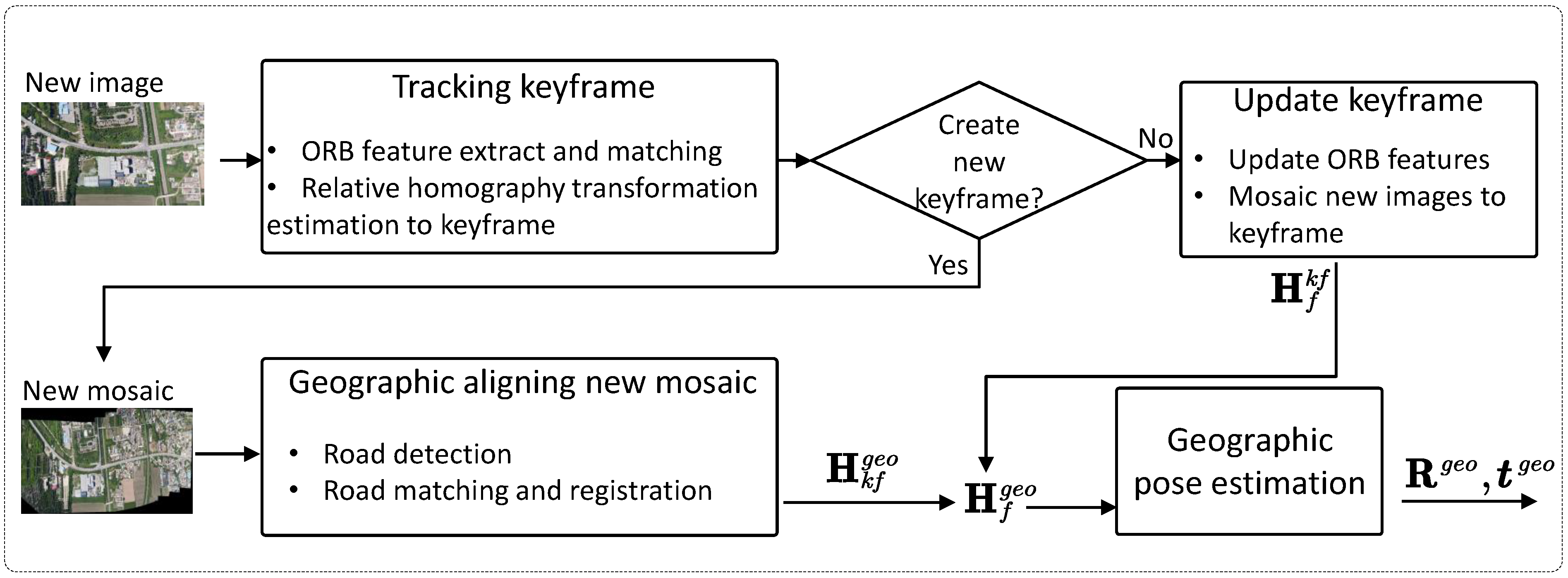
As demonstrated in Section 2.1, the geographic position of the camera can be computed once the aerial image is aligned to a georeferenced road map, and the homography transformation between them is estimated. For practical applications, the estimation of the camera geographic position must run in real time, which cannot be achieved using the road network alignment-based method, since road network alignment is time-consuming. However, as shown in our previous work [30], it is possible to achieve real-time alignment to the georeferenced road map when combining it with the relative transformation estimation computed from the ORB feature [31] matching to adjacent frames. Thus, we design a real-time geolocalization pipeline for UAVs by combining the relative transformation estimation from adjacent frames and geographic alignment to a given georeferenced road map.
As shown in Figure 2, the proposed road network alignment-based geolocalization method includes two threads: the geographic position estimation thread and the road network alignment thread.
Geographic position estimation thread: We use the method proposed in our previous work [30] to estimate relative homography transformation to a local reference keyframe. Different from the method in [30], we stitch the RGB image instead of detecting and stitching roads in each frame into a road mosaic image to achieve faster estimation. Thus, we can estimate the transformation between the current frame and the local reference frame (usually the first frame sent to the thread) and expend the mosaic of the scene in real time. With the geographic alignment result from the road network alignment thread, the homography transformation between the current frame and the georeferenced road map can be computed as . The geographic position of the camera is then estimated using the method proposed in Section 2.2 and refined using the method in Section 2.3. Once the current frame moves too far from its reference keyframe, a new keyframe will be created, and the old keyframe will be sent to the road network alignment thread.
Road network alignment-based geographic alignment thread: Upon receiving the keyframe from the geographic position estimation thread, road detection is conducted on the RGB image mosaic of the keyframe. A global road network feature search is performed for the first keyframe, or the homography transformation refining is conducted using the initial geographic alignment estimation from the geographic position estimation thread for the later keyframes using both of the methods proposed in our previous work [20]. Thus, the optimized transformation between the keyframe and the georeferenced road map can be obtained and is then used to update the transformation between the local reference frame and the georeferenced road map using .
3. Results
We performed experiments on both synthetic and real flight aerial image datasets to evaluate the performance of the proposed algorithm. In both experiments, we focused on evaluating the accuracy of the geographic positions of UAVs estimated using different methods. The geolocalization accuracy was measured using the total translation error in the X (longitude) and Y (latitude) directions between the estimated geographic position and the ground truth. The performance of the proposed method was compared with the commonly used position estimation method [2,3,4,12,21], where the projection point of the center point in the aerial image under the estimated homography transformtion is used as the position of the camera.
3.1. Experiment on Synthetic Aerial Image Dataset
In the experiment on the synthetic aerial image dataset, the synthetic “multi-poses dataset” reported in our previous work [19] was used to test the position estimation accuracy under different UAV poses. In the synthetic “multi-poses dataset”, 100 positions were selected randomly, and 10 aerial images, of which the yaws and rolls were kept the same while the pitches were varied from to , were generated in each position. We used the road match algorithm in [19] to estimate the homography transformation between the aerial images and the reference road map, and we then estimated the geographic position of the camera using the proposed method. The error was computed as , where and are the ground truth and estimated horizontal position of the UAV, respectively. We denote the result estimated with the proposed initial solution as , the result optimized with the pose refining procedure as , and the result computed with the projection point of the center point in the aerial image as . The result is reported in Figure 3.
3.2. Experiment on Real Flight Aerial Image Dataset
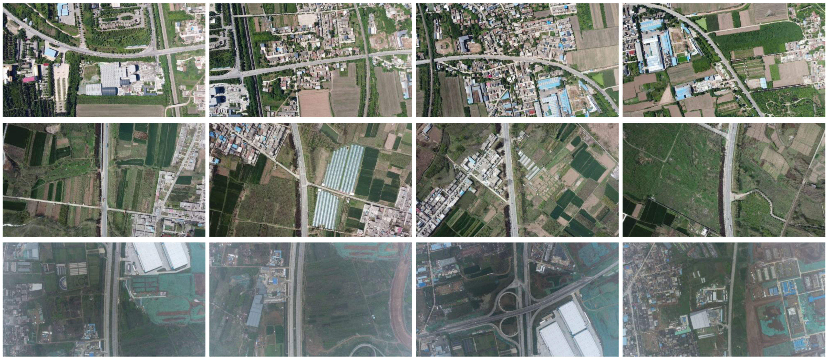
In the experiment, we captured three real flight videos with the DJI M300-RTK UAV in different scenes. The videos were captured with a straight-down-looking camera, while the UAV was operated under the control of a UAV manipulator. The manipulator operated from a car following the UAV, thereby ensuring that the UAV was within a safe control distance. The original resolutions of the videos were , and they were resized to in our experiments. The frames per second (FPS) of the original videos were 30. The positions of each frame were measured with using real-time kinematic (RTK) equipment mounted on the UAV and taken as the ground truth. The flight altitudes of the three videos were 500 m, 450 m, and 800 m, the maximum speeds were all 10 m/s, the total flight times were all about 170 s, and the lengths of the trajectory were about 1580 m, 1640 m and 1430 m. The detailed flight information for the three flights is summarized in Table 1. The three videos were caputred in different environmental conditions. Video A was captured in the city area, while the other two videos were captured in a suburb where the roads were sparser compared to those in video A. And video C was caputred on a foggy day, while the other two videos were caputred on sunny days. Thus, the three videos are representative. Some frames from the three videos are shown in Figure 4.
We downloaded the reference satellite map from a Google satellite map, cut it into small tiles, extracted the road map using the method in [14] in each tile, merged these road map tiles into a whole road map, and took the generated whole road map as our reference road map. The reference road map was expressed in the Mercator projection coordinate system (EPSG 3857) with the GSD of 1.0 m/pixel.
We then performed geolocalization experiments on the real flight aerial image dataset using the method described in Section 2.4. All the experiments were conducted on Nvidia Xavier AGX, which contains an 8-core NVIDIA Carmel Armv8.2 CPU and 32G of RAM, which can provide computility of up to 32 tera operations per second (TOPS) with a power consumption of no more than 30 W.
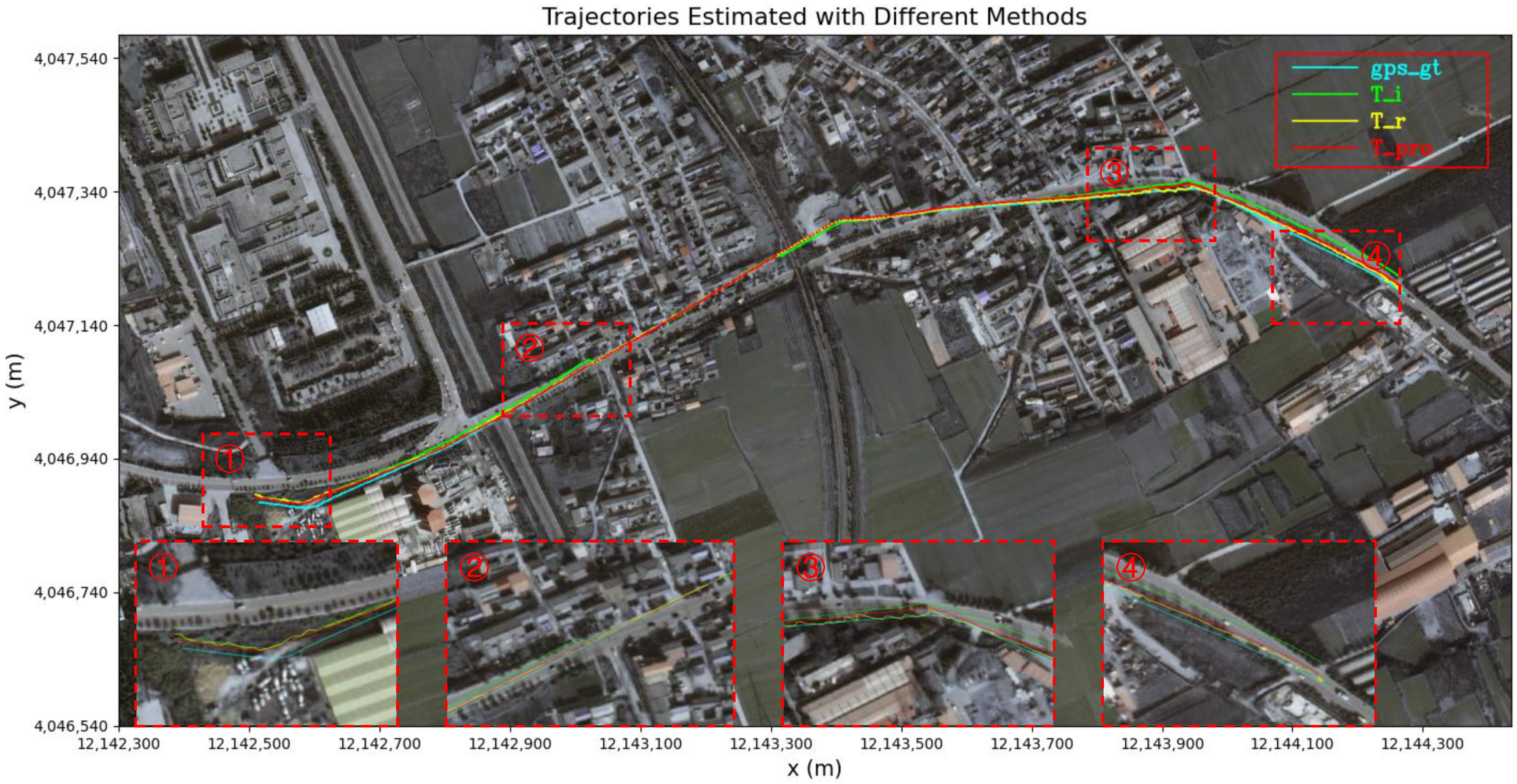
The geolocalization trajectories of the UAV for the three videos were recorded, and the geolocalization errors were computed and are shown in Figure 5. As can be seen, the proposed method (with the pose refining procedure) achieved the smallest geolocalization error in most cases in all three flights. To visually illustrate the trajectories estimated by different methods, we present the trajectories estimates from three different methods among the satellite map in Figure 6. The minimums, maximums, means, and medians of the geolocalization errors for the three geographic position estimation methods are shown in Table 2. It can be seen from Table 2 that the maximums, means, and medians of the geolocalization errors estimated using the proposed method (with the pose refining procedure) were minimal in all the three flights, which indicates the high accuracy of the proposed method.
The running time of the proposed method, which includes the time to compute the initial solution and the time to optimize the estimated pose, is also recorded and is shown in Table 3. The average running times of the geographic position estimation for the three flights were all less than 17 ms. The total time to process one frame was about 100 ms, including the time to estimate relative pose based on the ORB feature (about 40 ms), the time to extract the road (about 35 ms), and the time to estimate the geographic pose (about 17 ms), which means that the proposed road network alignment-based geolocalization method can run in about 10 Hz in practical applications, which is comparable with that of the GPS.
4. Discussion
Results from experiments conducted on both synthetic and real-flight datasets conclusively show that the proposed method adeptly and accurately estimates the geographic position of the UAV, irrespective of whether the camera’s optical axis is perpendicular to the ground.
The result on synthetic aerial image dataset shown in Figure 3 demonstrates that the maximum values and medians of the errors of the geographic positions estimated using the proposed initial solution were less than 10 m and 5 m, respectively, and they were reduced to 4 m and 2 m, respectively, after using the proposed pose refining procedure under all poses. This suggests that the proposed geographic position estimation method can estimate accurate geographic positions and that the proposed pose refining algorithm is effective in reducing the positioning error. The position errors estimated using the projection point increased rapidly with the pitch and reached tens of meters, even when the pitch was as small as , which means the method works only when the camera is nadir. The positioning accuracy after using the pose refining procedure improved slightly with the increase in pitch, which mainly benefits from the larger visual field under a larger pitch. In such cases, more roads are observed and provide more constraints for the pose optimization.
In the analysis of three real-flight aerial image sequences, notable reductions in position estimation errors were observed, exemplified by significant decreases at specific time points, such as 48.0 seconds and 77.5 seconds, as illustrated in Figure 5A, which were mainly due to successful road mosaic georeferencing. Since the image mosaicking algorithm computes the homography transformations of the image sequence in a recursive manner, there existed error accumulation in the estimated homography transformations. In other words, the accuracy of the estimated homography transformation improved as a frame got closer to its corresponding georeferenced keyframe. This phenomenon leads to abrupt decreases in positioning errors estimated with projection point. It indicates that estimating the position with the projection point is sensitive to the error in the computing homography transformation. Even though the proposed initial solution was also sensitive to the homography transformation estimation error, the error could be reduced effectively using the pose refining procedure in most cases, thus making our complete position estimation algorithm robust to homography transformation estimation noise.
There existed differences in the geographic position estimation accuracy in the three flights. The differences may mainly come from two aspects: the flight height and the density of road in the scene. Generally speaking, more observed roads can provide more constraints when estimating the homography transformation and refining the camera pose. When the roads of the scene are denser, more roads may be captured by the camera. As is shown in Figure 4, among the three flights, the road of the scene in flight A was much denser than that in B and C, thus resulting in the most accurate geographic position estimation. Also, a relatively high height may improve the estimation accuracy because the field of view is larger and more roads may be captured by the camera when the UAV flies at a relatively high height. Nevertheless, aerial images captured at higher flight altitudes exhibit a lower GSD, which is a factor that tends to marginally decrease the accuracy of the geographic position estimation.
5. Summary and Conclusions
In this paper, we concentrated on estimating the geographic position of the UAV with road network alignment in GPS-denied environments. We proposed a two-stage approach to estimate the UAV’s position in a given geographic coordinate system after successfully georeferencing images obtained by the UAV. The optimal initial solution of the camera pose that minimizes the Frobenius norm distance between the homography transformation estimated with road network alignment and that computed with the camera pose was first deduced and then refined further by solving the optimization problem that minimizes the alignment error between the observed road map and the reference road map. Experiments demonstrate that the proposed method can compute a more accurate geographic position and is less sensitive to the homography transformation estimation error in comparison to the commonly used method that estimates the geographic position using the projection point of the aerial image center, which works only when the camera is nadir. In the proposed method, it was assumed that all observed roads lay on the same horizontal plane, which holds in most but not all scenes, such as winding mountain roads. We plan to explore more general methods to address this issue in future research.
Author Contributions
Conceptualization, Y.L. and S.W.; methodology, Y.L. and D.Y.; software, Y.L. and L.S.; validation, Y.L. and D.Y.; formal analysis, Y.L. and D.M.; investigation, Y.L., D.Y. and D.M.; resources, D.Y.; data curation, Y.L. and D.Y.; writing—original draft preparation, Y.L.; writing—review and editing, Y.L.; visualization, Y.L.; supervision, D.Y.; project administration, S.W. and D.Y.; funding acquisition, Y.L., D.Y. and S.W. All authors have read and agreed to the published version of the manuscript.
Funding
This paper is supported by the National Key R&D Program of China (2022YFA1004100) and the National Natural Science Foundation of China (Grant Nos. 42301535, 61673017, 61403398).
Data Availability Statement
Data are contained within the article.
Conflicts of Interest
The authors declare no conflicts of interest.
References
- Patoliya, J.; Mewada, H.; Hassaballah, M.; Khan, M.A.; Kadry, S. A robust autonomous navigation and mapping system based on GPS and LiDAR data for unconstraint environment. Earth Sci. Inf. 2022, 15, 2703–2715. [Google Scholar] [CrossRef]
- Conte, G.; Doherty, P. Vision-based unmanned aerial vehicle navigation using geo-referenced information. EURASIP J. Adv. Signal Process. 2009, 2009, 387308. [Google Scholar] [CrossRef]
- Shan, M.; Wang, F.; Lin, F.; Gao, Z.; Tang, Y.Z.; Chen, B.M. Google map aided visual navigation for UAVs in GPS-denied environment. In Proceedings of the 2015 IEEE International Conference on Robotics and Biomimetics, Zhuhai, China, 6–9 December 2015; pp. 114–119. [Google Scholar]
- Yol, A.; Delabarre, B.; Dame, A.; Dartois, J.E.; Marchand, E. Vision-based absolute localization for unmanned aerial vehicles. In Proceedings of the 2014 IEEE/RSJ International Conference on Intelligent Robots and Systems, Chicago, IL, USA, 14–18 September 2014; pp. 3429–3434. [Google Scholar]
- Goforth, H.; Lucey, S. GPS-denied UAV localization using pre-existing satellite imagery. In Proceedings of the 2019 IEEE International Conference on Robotics and Automation, Montreal, QC, Canada, 20–24 May 2019; pp. 2974–2980. [Google Scholar]
- Nassar, A. A deep CNN-based framework for enhanced aerial imagery registration with applications to UAV geolocalization. In Proceedings of the 2018 IEEE Conference on Computer Vision and Pattern Recognition Workshops, Salt Lake City, UT, USA, 18–22 June 2018; pp. 1513–1523. [Google Scholar]
- Wu, L.; Hu, Y. Vision-aided navigation for aircrafts based on road junction detection. In Proceedings of the 2009 IEEE International Conference on Intelligent Computing and Intelligent Systems, Shanghai, China, 20–22 November 2009; pp. 164–169. [Google Scholar]
- Dumble, S.J.; Gibbens, P.W. Airborne vision-aided navigation using road intersection features. J. Intell. Robot. Syst. 2015, 78, 185–204. [Google Scholar] [CrossRef]
- Chang, C.H.; Chou, C.N.; Chang, E.Y. CLKN: Cascaded Lucas-Kanade networks for image alignment. In Proceedings of the 2017 IEEE Conference on Computer Vision and Pattern Recognition, Hawaii Convention Center, Honolulu, HI, USA, 21–26 July 2017; pp. 2213–2221. [Google Scholar]
- Simonyan, K.; Zisserman, A. Very deep convolutional networks for large-scale image recognition. arXiv 2014, arXiv:1409.1556. [Google Scholar]
- Kinnari, J.; Verdoja, F.; Kyrki, V. Season-Invariant GNSS-Denied Visual Localization for UAVs. IEEE Robot. Autom. Lett. 2022, 7, 10232–10239. [Google Scholar] [CrossRef]
- Hao, Y.; He, M.; Liu, Y.; Liu, J.; Meng, Z. Range–Visual–Inertial Odometry with Coarse-to-Fine Image Registration Fusion for UAV Localization. Drones 2023, 7, 540. [Google Scholar] [CrossRef]
- DeTone, D.; Malisiewicz, T.; Rabinovich, A. SuperPoint: Self-Supervised Interest Point Detection and Description. In Proceedings of the 2018 IEEE/CVF Conference on Computer Vision and Pattern Recognition Workshops (CVPRW), Salt Lake City, UT, USA, 18–22 June 2018; pp. 337–33712. [Google Scholar]
- Paszke, A.; Chaurasia, A.; Kim, S.; Culurciello, E. Enet: A deep neural network architecture for real-time semantic segmentation. arXiv 2016, arXiv:1606.02147. [Google Scholar]
- Zhang, Z.; Liu, Q.; Wang, Y. Road Extraction by Deep Residual U-Net. IEEE Geosci. Remote Sens. Lett. 2018, 15, 749–753. [Google Scholar] [CrossRef]
- Hua, Y.; Marcos, D.; Mou, L.; Zhu, X.X.; Tuia, D. Semantic Segmentation of Remote Sensing Images With Sparse Annotations. IEEE Geosci. Remote Sens. Lett. 2022, 19, 1–5. [Google Scholar] [CrossRef]
- Hu, M.-K. Visual pattern recognition by moment invariants. IRE Trans. Inf. Theory 1962, 8, 179–187. [Google Scholar]
- Máttyus, G.; Fraundorfer, F. Aerial image sequence geolocalization with road traffic as invariant feature. Image Vis. Comput. 2016, 52, 218–229. [Google Scholar] [CrossRef]
- Li, Y.; Yang, D.; Wang, S.; He, H.; Hu, J.; Liu, H. Road-network-based fast geolocalization. IEEE Trans. Geosci. Remote Sens. 2021, 59, 6065–6076. [Google Scholar] [CrossRef]
- Li, Y.; Wang, S.; He, H.; Meng, D.; Yang, D. Fast aerial image geolocalization using the projective-invariant contour feature. Remote Sens. 2021, 13, 490. [Google Scholar] [CrossRef]
- Wang, T.; Zhao, Y.; Wang, J.; Somani, A.K.; Sun, C. Attention-based road registration for GPS-denied UAS Navigation. IEEE Trans. Neural Netw. Learn. Syst. 2021, 32, 1788–1800. [Google Scholar] [CrossRef] [PubMed]
- Henriques, J.F.; Xavier, J.M.F. Motion and Structure from Motion in a Piecewise Planar Environment. Int. J. Pattern Recognit. Artif. Intell. 1998, 2, 742–748. [Google Scholar]
- Malis, E.; Vargas, M. Deeper Understanding of the Homography Decomposition for Vision-Based Control; Research Report-6303; INRIA: Le Chesnay-Rocquencourt, France, 2007; p. 90. [Google Scholar]
- Fusiello, A.; Trucco, E.; Verri, A. A compact algorithm for rectification of stereo pairs. Mach. Vis. Appl. 2000, 12, 16–22. [Google Scholar] [CrossRef]
- Nister, D. An efficient solution to the five-point relative pose problem. IEEE Trans. Pattern Anal. Mach. Intell. 2004, 26, 756–770. [Google Scholar] [CrossRef] [PubMed]
- Li, S.; Xu, C. A Stable Direct Solution of Perspective-Three-Point Problem. Int. J. Pattern Recognit. Artif. Intell. 2011, 25, 627–642. [Google Scholar] [CrossRef]
- Lepetit, V.; Moreno-Noguer, F.; Fua, P. EPnP: An Accurate O(n) Solution to the PnP Problem. Int. J. Comput. Vis. 2009, 81, 155–166. [Google Scholar] [CrossRef]
- Hartley, R.I.; Zisserman, A. Multiple View Geometry in Computer Vision; Cambridge University Press: Cambridge, UK, 2004. [Google Scholar]
- Felzenszwalb, P.; Huttenlocher, D. Distance Transforms of Sampled Functions; Technical Report; Cornell University: Ithaca, NY, USA, 2004. [Google Scholar]
- Li, Y.; He, H.; Yang, D.; Wang, S.; Zhang, M. Geolocalization with aerial image sequence for UAVs. Auton. Robot. 2020, 44, 1199–1215. [Google Scholar] [CrossRef]
- Rublee, E.; Rabaud, V.; Konolige, K.; Bradski, G. ORB: An efficient alternative to SIFT or SURF. In Proceedings of the 2011 International Conference on Computer Vision, Barcelona, Spain, 6–13 November 2011; pp. 2564–2571. [Google Scholar]
Figure 1.
Definition of coordinate systems.

Figure 2.
Pipeline of the proposed road network alignment-based real-time geolocalization method.

Figure 3.
Position estimation error on synthetic aerial image dataset. Here, ‘’ is the result estimated with the proposed initial solution; ‘’ is the result after using the pose refining procedure, and ‘’ is the result computed with the projection point of the center point in the aerial image under the estimated homography transformation.

Figure 4.
Several representative frames from the three real flight videos. Images in the 1st, 2nd, and 3rd row are from video A, video B, and video C, respectively.
Figure 4.
Several representative frames from the three real flight videos. Images in the 1st, 2nd, and 3rd row are from video A, video B, and video C, respectively.

Figure 5.
Position estimation error on real flight aerial image dataset. The errors of trajectory for video A, B and C are shown in subfigure (A), (B) and (C) respectively.
Figure 5.
Position estimation error on real flight aerial image dataset. The errors of trajectory for video A, B and C are shown in subfigure (A), (B) and (C) respectively.

Figure 6.
Camera trajectories of flight A on satellite map (in EPSG 3857).


Table 1.
Flight parameters for the real flight dataset.
| Altitude (m) | Maximum Speed (m/s) | Length (m) | Time (s) | |
|---|---|---|---|---|
| A | 500 | 10 | 1580 | 170 |
| B | 450 | 10 | 1640 | 170 |
| C | 800 | 10 | 1430 | 174 |
Table 2.
Statistic features of geolocalization error from three geographic position estimation methods. Best results are highlighted in bold.
Table 2.
Statistic features of geolocalization error from three geographic position estimation methods. Best results are highlighted in bold.
| Minimum (m) | Maximum (m) | Mean (m) | Median (m) | ||
|---|---|---|---|---|---|
| A | 0.07 | 28.75 | 10.00 | 7.51 | |
| 0.41 | 18.66 | 5.46 | 3.97 | ||
| 0.12 | 18.75 | 7.96 | 6.23 | ||
| B | 2.42 | 51.03 | 23.47 | 22.81 | |
| 2.07 | 34.60 | 11.93 | 12.28 | ||
| 1.19 | 41.49 | 16.37 | 15.78 | ||
| C | 0.13 | 56.75 | 20.11 | 13.07 | |
| 0.33 | 26.84 | 10.91 | 9.47 | ||
| 1.11 | 35.60 | 14.12 | 11.91 |
Table 3.
Statistic features of running time.
| Maximum (ms) | Mean (ms) | Median (ms) | |
|---|---|---|---|
| A | 33.06 | 16.10 | 15.20 |
| B | 37.88 | 15.43 | 13.82 |
| C | 47.62 | 15.42 | 13.58 |
Disclaimer/Publisher’s Note: The statements, opinions and data contained in all publications are solely those of the individual author(s) and contributor(s) and not of MDPI and/or the editor(s). MDPI and/or the editor(s) disclaim responsibility for any injury to people or property resulting from any ideas, methods, instructions or products referred to in the content. |
© 2024 by the authors. Licensee MDPI, Basel, Switzerland. This article is an open access article distributed under the terms and conditions of the Creative Commons Attribution (CC BY) license (https://creativecommons.org/licenses/by/4.0/).
Share and Cite
MDPI and ACS Style
Li, Y.; Yang, D.; Wang, S.; Shi, L.; Meng, D. Geolocalization from Aerial Sensing Images Using Road Network Alignment. Remote Sens. 2024, 16, 482. https://doi.org/10.3390/rs16030482
AMA Style
Li Y, Yang D, Wang S, Shi L, Meng D. Geolocalization from Aerial Sensing Images Using Road Network Alignment. Remote Sensing. 2024; 16(3):482. https://doi.org/10.3390/rs16030482
Chicago/Turabian StyleLi, Yongfei, Dongfang Yang, Shicheng Wang, Lin Shi, and Deyu Meng. 2024. "Geolocalization from Aerial Sensing Images Using Road Network Alignment" Remote Sensing 16, no. 3: 482. https://doi.org/10.3390/rs16030482
Note that from the first issue of 2016, this journal uses article numbers instead of page numbers. See further details here.