
Manifestation of Gas Seepage from Bottom Sediments on the Sea Surface: Theoretical Model and Experimental Observations


1
A.V. Gaponov-Grekhov Institute of Applied Physics of the Russian Academy of Sciences, 603950 Nizhny Novgorod, Russia
2
Radiophysical Department, Lobachevsky State University of Nizhny Novgorod, 603105 Nizhny Novgorod, Russia
3
Tomsk State University, 634050 Tomsk, Russia
4
V.I. Ilyichov Pacific Oceanological Institute, Far Eastern Branch of the Russian Academy of Sciences, 690041 Vladivostok, Russia
*
Author to whom correspondence should be addressed.
Remote Sens. 2024, 16(2), 408; https://doi.org/10.3390/rs16020408
Submission received: 1 November 2023
/
Revised: 17 January 2024
/
Accepted: 18 January 2024
/
Published: 20 January 2024
Abstract
:The key area of the Arctic Ocean for atmospheric venting of CH4 is the East Siberian Arctic Shelf (ESAS). Leakage of methane through shallow ESAS waters needs to be considered in interactions between the biogeosphere and a warming Arctic climate. The development of remote sensing techniques for gas seepage detection and mapping is crucially needed for further applications in the ESAS and other areas of interest. Given the extent of the seepage areas and the magnitude of current and potential future emissions, new approaches are required to effectively, rapidly, and quantitatively survey the large seepage areas. Here, we consider the main features of gas seep detection on the sea surface in the characteristics of wind waves and radar signals. The kinematics of wave packets based on the kinetic equation for the spectral density of the wave action of surface waves is described. The results of a full-scale experiment on the remote radar observation of a model gas seep to the sea surface in the radar equipment signals are considered. The characteristic radar signatures of the gas seep in a wide range of hydrometeorological conditions, the parameters of which were recorded synchronously with the radar mapping, were determined. The results of the first radar observations of natural methane seeps on the ESAS are presented, and their radar contrasts are evaluated. The theoretical conclusions are in good qualitative agreement with the results of the model experiment and field studies and can be used for further research in aquatic areas with potential gas seepage, both of natural or anthropogenic origin, such as bubbling release from broken underwater gas pipelines.
1. Introduction
The need for the remote detection of gas bubbling release (called seeps) on the sea surface arises in the problems of monitoring gas leaks in underwater gas pipelines, including emergencies. With pipeline destruction, the gas seep intensity can be so high that it does not require the application of special means and methods for detection. However, there are many situations where the gas seep intensity is not high, and in most cases, gas bubbles do not reach the sea surface. This is a common situation for the entire World Ocean [1], except for several areas where strong methane ebullition was found [2].
The East Siberian Arctic Shelf (ESAS), which includes the Laptev Sea, the East Siberian Sea, and the Russian part of the Chukchi Sea, is the region of the World Ocean where more than 80% of the world’s predicted subsea permafrost and associated permafrost-related hydrates exist. The ESAS had not been considered to be a methane (CH4) source of hydrosphere or atmosphere because subsea permafrost, which underlies most of the ESAS, was believed, first, not to be conducive to methanogenesis and, second, to act as an impermeable lid, preventing CH4 escape through the seabed [3,4].
The discovery of elevated dissolved CH4 and an elevated atmospheric CH4 mixing ratio, and further geophysical studies [5,6,7], demonstrated that the most likely main source is year-round CH4 bubbling release through taliks (columns of thawed sediments within permafrost) from seabed CH4 reservoirs such as shallow hydrates and geological sources [7,8]. Such releases occur not only within the areas underlain by fault zones but also outside of them. This points to the permafrost’s failure to further preserve CH4 deposits in the ESAS. The total amount of carbon preserved within the ESAS as organic matter and ready-to-release CH4 from seabed deposits is predicted to be ~1400 Gt [6,9,10,11]. At the same time, the current annual emission of CH4 to the atmosphere lies in the range of 8–17 Tg and is on par with previous estimates of methane venting from the entire World Ocean [5,7,12]. The release of only a small fraction of this reservoir, which was sealed with impermeable permafrost for thousands of years, would significantly alter the annual CH4 budget and have global implications because the shallowness of the ESAS allows the majority of CH4 to pass through the “sulfate oxidation filter” in the surface sediments and water column and escape to the atmosphere [5,6,12,13,14]. Because the ESAS contains the largest and arguably most vulnerable stores of subsea CH4 [15], the inclusion of the ESAS source in global climate models should be considered a high priority. This amount of pre-formed gas preserved in the ESAS suggests a potential for the possible massive and abrupt release of CH4 due to destabilizing hydrates or free gas accumulations beneath the permafrost. This release requires only a trigger like subsea permafrost thawing and/or seismotectonic activity [16]. As a result, the development of methods for the remote sensing and mapping of methane seeps is a quite significant part of the complex studies targeted at a better understanding and quantification of the increasing CH4 release in the ESAS seepage areas.
The research on gas seepage is also being carried out in other regions of the World Ocean. The book [17] provides a comprehensive study of seeps in the South China Sea, including using seismoacoustic and hydroacoustic sounding, but manifestations on the sea surface are not considered. The ascent rate of gas bubbles was recorded using the particle image velocimetry method. Ascent velocities of about 0.3 m/s were registered. The article [18] conducted a study of seepage in the Gulf of Mexico. In addition to hydroacoustic data obtained from the research vessel, two Radarsat-2 satellite SAR images, discussed in detail in [19], were considered. It should be noted that the seep area was detected by oil film contamination on the surface, which is associated with the release of oil along with gas bubbles to the sea surface. To detect oil pollution, automatic algorithms for their identification have now been proposed [20] and for cases of oil leaking from the seabed, the problem can be considered solved. However, there are cases when only gas in the form of bubbles leaks from the bottom, and this case is considered in this work.
Bubbles in the water column usually come from seeps on the sea floor and can be detected using backscattered images of bubbles because there is a pronounced acoustic impedance difference between the water and bubbles [21]. In places, bubbles release as a vigorous flow that often reaches the sea surface; on echograms, such bubble plumes create specific flare-like images. The highest rates (30–176 g m−2 d−1) likely represent the maximum emissions currently taking place from the outer shelf [7]. The observed range in CH4 emissions associated with different degrees of subsea permafrost disintegration implies substantial and potent emission enhancement in the ESAS as the process of subsea permafrost thawing progresses coastward with time [7]. While it is still unclear how quickly CH4 flux rates will change, the current process of Arctic warming and associated sea ice loss will accelerate this process. Given the extent of the seepage areas and the magnitude of current and potential future emissions, new approaches are required to effectively, rapidly, and quantitatively survey the large seepage areas.
To observe and map gas seepage areas, it is possible to employ remote sensing techniques. In most cases, a gas seep is detected by optical images of the ice sheet, in which the ice areas saturated with accumulated gas contrast with the background ice [22]. However, if the water surface is ice-free and covered with wind waves, the problem of detecting weak gas seeps seems difficult and is primarily related to the transformation of the spectrum of short wind waves in the field of turbulent currents created by a buoyant bubble jet. The complexity of the problem in this formulation is determined primarily by a wide range of variations in the characteristics of wind waves, parameters of stratification of the water column and currents, and, as far as the authors know, this problem cannot be considered as solved. The solution to the problem is complicated by the relatively small size of the area of the gas seep to the sea surface, which is determined by the transverse size of the gas jet and its intensity, as well as the possible unsteadiness of the process. The effect of blocking surface waves by injecting gas bubbles beneath the surface has been known for more than 100 years. Theoretical and experimental investigations have shown that the surface currents set up by gas injection and currents set up by water jets have almost the same wave-blocking effect. It has been concluded that the bubbles as such have at most a very small effect on the wave motion [23,24].
This paper aims at a comprehensive theoretical and experimental study of the characteristic features of the gas seep in the structure of surface waves, and the manifestation of these features in sensing radar signals. To achieve this goal, the paper starts with a theoretical model of the wind wave transformation in the current field created by a buoyant gas jet on the sea surface. This model is based on the kinetic equation for the wave action spectral density. However, the direct influence of bubbles on waves is not considered; we consider only the influence of large-scale inhomogeneous current, which can be remotely determined. After that, the theoretical results are compared with the results of a full-scale experiment on the remote sensing of an artificial gas seep, modeled from a stationary oceanographic platform in the Black Sea in 2021. Finally, the results of the remote sensing of natural methane seeps obtained in the East Siberian Sea during the 82nd cruise of the research vessel “Akademik Mstislav Keldysh” [25] are presented. All theoretical and experimental conclusions are compared.
2. Theoretical Model
The effect of inhomogeneous subsurface currents on wind waves has been discussed for several decades [26]. Interest in this problem has especially increased due to the development of new remote methods and means of detecting the manifestation of currents on the ocean surface. The most interesting source of inhomogeneous currents is probably the wave motion in the stratified fluid, namely, internal waves. Proceedings of the Institute of Applied Physics of the Russian Academy of Sciences were devoted to the theoretical and experimental study of the effects of large-scale internal waves on the sea surface [26]. The transformation of the wind wave spectrum in the range of decimeters and longer surface waves under the action of an inhomogeneous current is analyzed by numerical methods based on the kinetic equation for the spectral density of the wave action of surface waves [27]. In the decimeter and meter ranges of surface wavelengths, the determining role is played by a mechanism related to the change in the kinematic parameters of surface waves under the action of an inhomogeneous current.
To describe the kinematics of waves on an inhomogeneous current, the concept of a spatial spectrum is used. The evolution of wind wave spectra in the framework of the kinematic model is described by the kinetic equation for the spectral density of the wave action of surface waves: , where is the gravitational acceleration, (see for example [27]):
where the following applies:
Here is the surface wave frequency. This paper considers quasi-stationary currents formed by a buoyant gas flow. With allowance for the capillary effect, the dispersion ratio will take the following form: , where is the coefficient of the surface tension of water and is the water density.
The term in Equation (1) describes the effect of wind and viscosity on surface waves and takes into account their nonlinearity. The relaxation approximation is the most common, where is written in the following form: , where is the spectral density of the wave action in the unperturbed state and is the increment of the increase of wind waves.
The system of Equation (2) determines the type of trajectory of surface wave packets in space . The change of N along the trajectory is determined by Equation (3).
In the short-wave (millimeter and centimeter) range of wind wavelengths, the film mechanism of the effect of inhomogeneous currents on wind ripples [28] and the nonlinear mechanisms of energy transfer from the long-wave region of the wind wave spectrum to short waves are most effective [29].
2.1. Problem Statement
Let the buoyant gas flow, carrying along the fluid from the water column, reach the sea surface and spread radially [30]. Then the current field on the sea surface can be represented in the following form:
where is the buoyant jet radius, is the characteristic velocity of the fluid carried along by the gas flow, and
is a unit vector along . Then the system of Equation (2), which determines the trajectory of the wave rays in the Cartesian plane will be represented as follows:
The solution of the system of Equation (4) is the trajectories of wave rays, the analysis of which makes it possible to observe the refraction and blocking of wave packets. This problem is similar to the classical cylinder flow problem. Let a plane wavefront with a wave number fall on the perturbation region. Obviously, for wind waves with lengths , where is the characteristic scale of the inhomogeneity of the current velocity on the surface, this model will not be applicable, hence the limitation on the wavelength as it appears from above, and for the wave number it is from below. Determine as the distance at which the current velocity drops by e times, then .
2.2. Simulation Results
When a plane wavefront with a wave number falls, different scenarios will develop depending on the group velocity (for simplicity, let us consider gravity waves) of the wave packet, where is the projection of the current velocity vector on the propagation direction of . When the group velocity is equal to zero, the condition of blocking and reflection of the wavefront for wave numbers arises. When waves pass through the perturbation region, refraction with the formation of an interference pattern behind the perturbation region occurs. Characteristic patterns of wave rays for two regions of wave number values, conventionally “long” and “short” waves, are shown in Figure 1. A symmetrical pattern of the behavior of wave rays is observed. For “long” waves, a low-contrast interference pattern is formed behind the perturbation region, which, with allowance for the continuous wave spectrum, is hardly possible to detect by remote methods. However, for “short” waves, a shaded area without waves (slick) is formed above the perturbation region due to the effects of blocking and reflection. As can be seen in Figure 1b, after blocking, the wave packets move to another branch of the dispersion curve, which allows them to overcome the current gradient due to a strong increase in the wave number and, consequently, the group velocity. However, it should be noted that this effect cannot be implemented due to the restriction on the steepness of the waves (kA). Initially, for a wave packet with a wave number the spectral density of the wave action N0 is preserved with an increase in the wave number on the counter-current (in fact, it is determined by Equation (3), but the time scale of the change in the wave number is much less than the relaxation time ). Thus, the wave is becoming steeper, i.e., the value of kA increases and breaks after reaching the restriction. This occurs at the upwind perturbation boundary. As can be seen in Figure 2a, the change in the wave number can reach two orders of magnitude; accordingly, kA also changes. It is quite difficult to perform a numerical solution to Equation (3); however, a qualitative picture of the wind wave field transformation is formed from the analysis of the ray pattern and the reasoning made. Figure 1b shows that the size of the slick region is larger than the radius of the buoyant jet . When a wave packet propagates in the counter-current, its wave number begins to increase, and the blocking conditions can be reached earlier. After analyzing Figure 1b, it can also be concluded that in the upwind region of the perturbation created by the buoyant gas flow, where waves are blocked and reflected, conditions for the growth of their amplitude and breakdown arise, thereby forming a surface area with increased roughness, i.e., suloy. In combination with the rounded slick described above, the horseshoe-shaped suloy is a characteristic sign of gas seep on a rough water surface during remote detection. Considering that the short-wave range of the wind wave spectrum is crucial for remote radar sensing methods, conditions for remote detection of such a perturbation arise.
For an X-band radar, the waves determining backscattering satisfy the Bragg ratio [31] , where is the radar wave number, and is the grazing angle. Such a condition for low grazing angles is satisfied by waves with lengths of 1.6 cm, for which Equation (3) was solved. For this, a system of Equation (4) with time reversal was solved on a uniform grid of initial conditions [ for the wave vector ]. Thus, the coordinates to which the Bragg waves come from an undisturbed section of the sea surface along the wave rays from (4) were set. Next, Equation (3) is solved for each wave ray, along which the spectral density of the wave action N is calculated. The Naval Research Laboratory spectrum was used as an undisturbed spectrum [32], and the increment of the increase of wind waves was calculated using the Hughes formula [33]. It should be noted that the choice of these parameterizations was determined solely for reasons of convenience of calculations. Choosing other parameterizations will not qualitatively change the obtained results. The calculation was carried out for a wind speed and . The calculation results in the form of the ratio of the spectral density of Bragg waves to the value undisturbed by the current are shown in Figure 2b. In the area above the gas flow, conditions are created for blocking waves, as described above, so that a complete absence of Bragg waves is observed. As the value of increases, this area will become larger. At the windward boundary, the spectral density of Bragg waves increases. This occurs because the energy of the longer-wavelength components of the spectrum is transferred, the wave number of which increases in the counter-current. The same calculations can be performed for all wave numbers in the wind wave spectrum. This picture also describes variations in the scattered radar signal in the Bragg scattering approximation. In real marine conditions, the scattering of radio waves will also involve breaking waves, which will increase radar contrasts from the windward side of the disturbance. Using Equation (3), this effect cannot be taken into account. The full spectrum transformed by an inhomogeneous current can be used to calculate the normalized radar cross-section, for example using the model [34].
Let us briefly outline the main features of the manifestation of underwater gas seeps on the sea surface in the presence of wind waves.
- At the upwind boundary of the gas seep on the water surface, conditions for an intense breaking of short waves arise. As a result, these waves do not go further. A semicircular band of increased roughness (suloy) is formed, framing the upwind part of the perturbation region.
- Short waves directly above the area of the gas seep to the water surface are almost absent. A rounded area of reduced roughness (a slick), which marks the place of the gas seep, is formed.
- The effect of the gas seep area on the water surface on long wind waves is weak. In turn, the effect of the long wave on the gas seep on the sea surface is significant.
- For the remote detection of the surface manifestation of the gas seep to the water surface, it is optimal to use radar equipment of the centimeter wavelength range capable of forming a spatial image.
- The area of the gas seep surface manifestation is several times larger than the gas jet diameter and depends on the parameters of the wind wave, the background current velocity, and the gas jet power.
3. Experimental Simulation
In order to experimentally verify the theoretical conclusions, a full-scale experiment on the remote sensing of a model gas seep in the Black Sea was conducted from the stationary oceanographic platform of the Marine Hydrophysical Institute of the Russian Academy of Sciences in the village of Katsiveli in 2021. The experiment consists of a periodic air supply using a compressor with a capacity of 130 L/min through a hose with a diameter of ½″, the open end of which was located at the bottom at a depth of about 40 m at a distance of approximately 100 m from the platform. The scheme of the experiment is shown in Figure 3.
After the air supply, the bubbles reached the surface, and a stationary pattern of surface manifestation was established (see the photo in Figure 3). After 20 min, the air supply stopped and the background situation, which was being recorded for 40 min, was restored. A continuous 24 h series of such experiments was performed, during which 24 generations of gas seep were conducted. It should be noted that work on the remote sensing of the model gas seep has been known since the early 2000s [35,36]; however, unfortunately, only a single experiment was conducted.
The radar scanning of the sea surface was performed with coherent circular radar operating in the X-band on horizontal polarization. The modulation band of the frequency-modulated radio signal with a carrier frequency f0 = 9.5 GHz was fm = 191 MHz. During one revolution of the radar antenna, a bright radar image of the sea surface in polar coordinates is formed. The resolution of the generated radar image in range and azimuth was about 1 m. Radar images of the sea surface in all 24 cases show characteristic signatures of the manifestation of a gas seep over the generation area; however, it is impossible to select an automatic algorithm for their confident detection in the entire range of observed hydrometeorological conditions (HMCs). A video compiled from a sequence of radar images during the experimental simulation can be found in the supplementary materials. HMCs, including the velocity and direction of the near-water wind (acoustic anemometer WindSonic Gill InstrumentsTM), wind wave parameters (wave measuring buoy DWR-G4 DatawellTM), as well as the velocity and direction of the current at various depths starting from 1 m (acoustic Doppler current profiler ADCP WorkHorse Monitor 1200 kHz RDITM), were recorded throughout the experiment. Figure 4 shows variations in the radar signatures of the manifestation of the gas seep on the sea surface at different HMCs. The following characteristic features can be distinguished.
A. With weak or moderate sea waves and a weak current, a local area of increased normalized radar cross-section (NRCS) is observed on the upwind side of the gas seep to the sea surface relative to the background values, and a reduced value of NRCS is observed on the downwind side. The shape of the signatures is symmetrical round or horseshoe-shaped.
B. With weak or moderate sea waves and strong currents, radar signatures are pulled in the current direction.
C. With strong sea waves, the signature contrast decreases, and it becomes difficult to distinguish the sign-variable contrast that occurs at a small-scale gas seep from a breaking long wind wave.
Characteristic signature sizes of about 20 m in diameter were observed in the experiment. An increase in the current velocity leads to an increase in size along the current direction. Increased wind leads to a decrease in the radar contrast of the gas seep area. Further, we consider the quantitative characteristics of radar signatures generated by the gas seep on the sea surface. The sea surface NRCS, when measured using radar, is calculated by the formula obtained by calibration with an angle reflector, where is the power of the received radar signal from the resolution element. The fragments of the radar images are shown in Figure 4 for HMCs from Table 1. Next, the NRCS maximum level is searched for, after which all NRCS values are averaged within radius r = 5 m to eliminate the effect of random interference related to micro-breakings and other objects leading to local signal amplifications. This value should characterize the maximum level in the signature . In order to obtain contrast, normalization to the average level of NRCS was performed over the entire fragment of the radar image or to the minimum level of NRCS , obtained by analogy with and characterizing the minimum level in the signature.
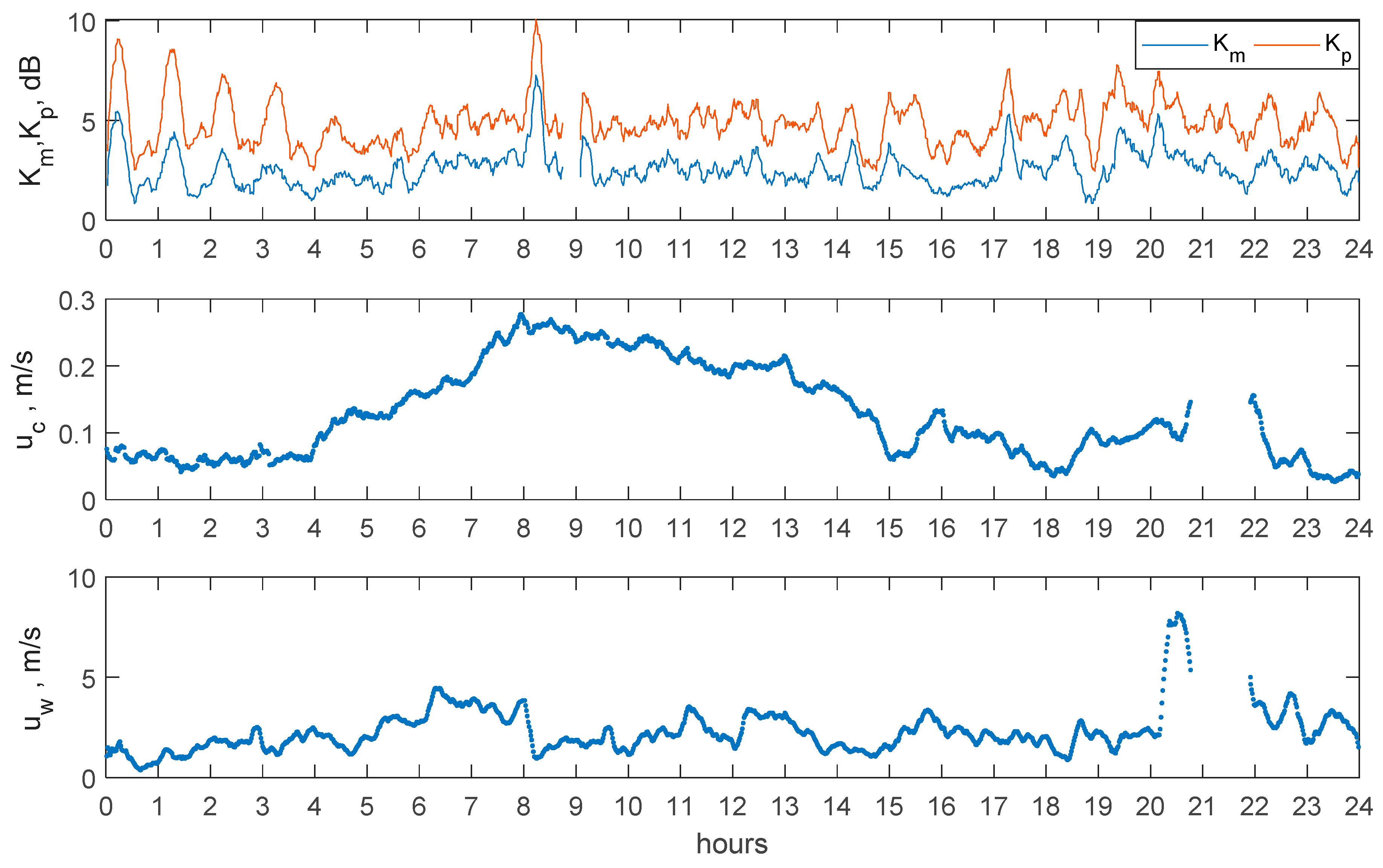
Figure 5 shows the radar contrasts and . The periodic variability of Km and Kp values is clearly visible almost throughout the entire diagram. The intervals during a 20 min period from the beginning of each hour in the diagram correspond to the compressor operating time. Background contrasts caused by the effect of a long wave, as well as by the dependence of the NRCS on the sensing angle and azimuth angle relative to the wind direction, which is characteristic even for a small image fragment, are approximately equal to 2 dB and 4 dB for Km and Kp, respectively.
At the level of background contrasts, the signature contrasts at the beginning of the diagram from 00:00 to 05:00 ranging from 2.5 dB to 5.5 dB for Km and from 5 dB to 9 dB for Kp are clearly distinguished. This time period corresponds to a weak wind and a weak current (Figure 5), although a swell with a characteristic length of about 60 m, which is significantly larger than the gas seep area, is present. Further, an increase in the current up to 30 cm/s and the wind up to 5 m/s, which, together with the swell, raises the background contrast to 3 dB and 5 dB for Km and Kp, respectively, and masks the signatures related to the gas seep. Starting at 14:00, the wind velocity significantly decreased, and the current velocity also began to decrease. A decrease in background contrasts to initial values is observed, and the contrasts of the desired signature become distinguishable.
4. Full-Scale Experiment
Experimental studies were performed during the 82nd scientific cruise of the RV “Akademik Mstislav Keldysh” organized by the Laboratory of Arctic Research, Pacific Oceanological Institute of the Far Eastern Branch of the Russian Academy of Sciences. One of the key objectives was to study vigorous methane seeps discovered in the East Siberian Sea onboard RV “Akademik Mstislav Keldysh” in 2019 (Semiletov, unpublished material).
The description of radar observations of sea waves and currents, ice fields, manifestations of internal waves, surface manifestations of gas seeps during the cruise, and data processing algorithms are given in [25]. This paper presents the results of observations of a real methane seep and its comparison with the results of theoretical calculations and model experiments given above. An important difference between the ship experiment and the one discussed above is the movement of the radar equipment carrier and the change in its orientation. When processing radar images received from the vessel, the images all are transferred to a common coordinate grid before averaging. With a sufficient number of averaged radar images, the wave processes on the sea surface will be smoothed out, and stationary objects, to which the surface manifestation of the gas seep can be attributed, on the contrary, will increase their contrast. Note that for such processing, it is desirable to have a high speed of space observation.
A map of the test area in the East Siberian Sea with the manifestation of natural gas seeps on the sea surface is shown in Figure 6. During the 82nd cruise, a geophysical mapping of the test area, as well as work on individual methane seeps while keeping the vessel at a point using thrusters, was performed. The map shows the research area and the path of the RV “Akademik M. Keldysh”. A photograph of the natural methane seep to the sea surface demonstrates the features described above.
During the radar operation from a weakly drifting vessel, the area of the methane seep is observed at the same or close azimuthal angles. The radar contrast of the hydrodynamic perturbation created by the methane seep to the surface depends significantly on the observation geometry. Figure 7 shows radar images of the sea surface averaged over 20 min, which show natural (a) and model (b) gas seeps. The areas of radar images with gas seeps are plotted with a dotted line. As for the case of a model experiment, in real conditions, a gas seep creates sea surface perturbations described by the theoretical model, and their characteristic radar signatures are similar (see Figure 4 and Figure 8). As a numerical criterion for the observability of the manifestation of a methane seep on the sea surface, we introduce the value R, defined as the ratio of the standard deviation of the value in the area of the surface manifestation of seeps to the standard deviation in a close but unperturbed surface area. The dependence of R on the wind velocity for two areas of methane seeps on the surface is shown in Figure 8c. For the first seep (seep No. 1), which was 150 m away from the RV, we obtained values of R higher than for the second seep (seep No. 2), which was located at a distance of 350 m. It can be seen that with an increase in wind velocity, R decreases, which leads to the impossibility of remote radar observation of the surface manifestation of seeps. The values of R are in the range of 2–4 dB, which corresponds to the ratio of the Km contrasts in the model seep to the background values observed in the model experiment (Figure 8c).
5. Discussion
Although the paper considers in detail the theoretical and experimental features of the disturbance of wind waves generated by gas seeps on the sea surface, which are in good qualitative agreement (paragraphs 1–5 of the section “Simulation Results” and paragraphs A and B of the section “Experimental Modeling”), the practical application of the obtained results for the remote detection of natural gas seeps using existing equipment installed on satellites can only be performed with difficulty. This is primarily due to the limitations of the equipment resolution, as well as the inability to temporarily accumulate signals reflected by the rough sea surface. On satellite images of the sea surface obtained by synthetic aperture radar in high-resolution mode, such as TerraSAR-X and RadarSat, cases of the detection of natural seeps under certain hydrometeorological conditions are possible. Such conditions include weak wind waves with no breakings, the absence of significant swells, and the absence of strong stratification preventing gas bubbles from reaching the sea surface. With allowance for the fact that shooting in high-resolution mode is performed on a commercial basis, only covers small areas, and the detection of the studied object strongly depends on hydrometeorological conditions, the use of such tools may be economically impractical at the moment.
The most appropriate remote sensing tool for detecting surface manifestations of gas seeps is a microwave circular radar, mounted on a carrier moving at a speed that allows one to scan the same area of the sea surface several times for subsequent accumulation of radar signal. This will enable one to eliminate wave motion and breakings, while stationary objects, on the contrary, will increase their contrast. Not only a vessel can act as a carrier of radar equipment, but also aviation and satellite carriers if the above condition is met. For aviation equipment, the installation of a scanning radar with a real aperture seems acceptable, given the relatively low speed of movement of the air carrier and low altitude. At the same time, for a satellite, the option of scanning radar equipment with real aperture is not suitable and it is necessary to use sequential SAR imaging from several satellites, for example, TanDEM-X. But it is better to have a large series of images for better averaging.
The object of the research considered in this work is the disturbance of wind waves generated by the release of gas to the sea surface, which is much more complicated than oil pollution on the sea surface, which has now been successfully detected, including in automatic mode [20]. Progress in the detection and identification of oil spills is associated with the emergence of new satellite instruments like polarizing synthetic aperture radar with high spatial resolution. The task considered in this article may be solved just as effectively with the advent of new tools, the requirements for which are formulated above.
6. Conclusions
The paper solves the problem of determining the main features of the manifestation of gas seeps to the sea surface in the area of wind waves and reflected radar signals. The main radar signatures of gas seeps have been determined in a wide range of hydrometeorological conditions within the framework of a model experiment and in real conditions in the East Siberian Sea. It is shown that the obtained theoretical conclusions are in good agreement with the results of full-scale modeling and full-scale experiments. The results of this work can be employed in conducting research in any aquatics with potential gas seepage, both of natural or anthropogenic origin, such as gas leakage from broken underwater gas pipelines. Also, the results of this article can help formulate requirements for advanced satellite and aviation radar equipment for detecting and mapping seeps, which is extremely important in modern conditions of global warming, especially for the Arctic region and the ESAS in particular.
It should be noted that the article considers only those gas seeps whose bubbles reach the sea surface. Most natural seeps are found in the water column and can be detected by hydroacoustic methods only. However, if the gas bubbles reach the sea surface and the seep is localized, then conditions are created for its detection by radar means. Based on the results of this work, it is difficult to conclude the minimum intensity of gas seeps, which can be detected by the disturbances they create in the field of wind waves. This is a multiparametric task, which includes the parameters of the stratification of the water column, the speed of current and wind, and the characteristics of background waves along with the intensity of the gas seepage. This task will be solved by the authors soon.
Supplementary Materials
The following supporting information can be downloaded at: https://www.mdpi.com/article/10.3390/rs16020408/s1, Video S1: Video edited from a sequence of radar images during the experimental simulation. All data can be obtained on request.
Author Contributions
Conceptualization, A.E. and I.K.; methodology, A.E., I.K. and A.M.; carrying out measurements, A.E., I.K., A.M. and I.S.; data processing and analysis, A.E.; writing—original draft preparation, A.E.; writing—review and editing, A.E., I.K. and I.S. All authors have read and agreed to the published version of the manuscript.
Funding
The model experiment and theoretical modeling were performed within the framework of the UNN state assignment (topic No. 0729-2020-0037). Radar research was supported by the Russian Science Foundation (grant No. 20-77-10081, https://rscf.ru/project/20-77-10081/). This field-based study was supported by the Ministry of Science and Higher Education of the Russian Federation (grant “Priority-2030”, Tomsk State University, grant 021-2021-0010), and by the Russian Science Foundation (grant: 21-77-30001).
Data Availability Statement
Data are contained within the article.
Acknowledgments
The authors express their gratitude to captain Yuri Gorbach and crew of the 82nd scientific cruise of the RV “Akademik Mstislav Keldysh” for productive joint work on the cruise.
Conflicts of Interest
The authors declare no conflicts of interest.
References
- Fleischer, P.; Orsi, T.H.; Richardson, M.D.; Anderson, A.L. Distribution of free gas in marine sediments: A global overview. Geo-Mar. Lett. 2001, 21, 103–122. [Google Scholar]
- Naudts, L.; Greinert, J.; Artemov, Y.; Staelens, P.; Poort, J.; Van Rensbergen, P.; De Batist, M. Geological and morphological settings of 2778 methane seeps in the Dnepr paleo-delta, northwestern Black Sea. Mar. Geol. 2006, 227, 177–199. [Google Scholar] [CrossRef]
- Shakhova, N.; Semiletov, I. Methane release and coastal environment in the East Siberian Arctic shelf. J. Mar. Syst. 2007, 66, 227–243. [Google Scholar] [CrossRef]
- Romanovskii, N.N.; Hubberten, H.-W.; Gavrilov, A.V.; Eliseeva, A.A.; Tipenko, G.S. Offshore permafrost and gas hydrate stability zone on the shelf of East Siberian Seas. Geo-Mar. Lett 2005, 25, 167–182. [Google Scholar] [CrossRef]
- Shakhova, N.; Semiletov, I.; Salyuk, A.; Yusupov, V.; Kosmach, D.; Gustafsson, O. Extensive methane venting to the atmosphere from the sediments of the east Siberian Arctic Shelf. Science 2010, 327, 1246–1250. [Google Scholar] [CrossRef] [PubMed]
- Shakhova, N.; Semiletov, I.; Leifer, I.; Rekant, P.; Salyuk, A.; Kosmach, D. Geochemical and geophysical evidence of methane release from the inner East Siberian Shelf. J. Geophys. Res. 2010, 115, C08007. [Google Scholar] [CrossRef]
- Shakhova, N.; Semiletov, I.; Sergienko, V.; Lobkovsky, L.; Yusupov, V.; Salyuk, A.; Salomatin, A.; Chernykh, D.; Kosmach, D.; Panteleev, G.; et al. The East Siberian Arctic Shelf: Towards further assessment of permafrost-related methane fluxes and role of sea ice. Philos. Trans. R. Soc. B 2015, 373, 20140451. [Google Scholar] [CrossRef] [PubMed]
- Steinbacha, J.; Holmstranda, H.; Shcherbakova, K.; Kosmachd, D.; Brüchert, V.; Shakhova, N.; Salyuk, A.; Sapart, C.J.; Chernykh, D.; Noormets, R.; et al. Source apportionment of methane escaping the subseapermafrost system in the outer Eurasian Arctic Shelf. Proc. Natl. Acad. Sci. USA 2021, 118, e2019672118. [Google Scholar] [CrossRef]
- Gramberg, I.S.; Kulakov, Y.N.; Pogrebitskiy, Y.Y.; Sorokov, D.S. Arctic Oil and Gas Super Basin; X World Petroleum Congress: London, UK, 1983; pp. 93–99. [Google Scholar]
- Soloviev, V.A.; Ginzburg, G.D.; Telepnev, E.V.; Mikhaluk, Y.N. Cryothermia and Gas Hydrates in the Arctic Ocean; Sevmorgeologia: Leningrad, Russia, 1987; 150p. (In Russian) [Google Scholar]
- Kvenvolden, K.A. Methane hydrates and global climate. Glob. Biogeochem. Cycles 1988, 2, 221–229. [Google Scholar] [CrossRef]
- Shakhova, N.; Semiletov, I.; Leifer, I.; Sergienko, V.; Salyuk, A.; Kosmach, D.; Chernykh, D.; Stubbs, C.; Nicolsky, D.; Tumskoy, V.; et al. Ebullition and storm-induced methane release from the East Siberian Arctic Shelf. Nat. Geosci. 2014, 7, 64–70. [Google Scholar] [CrossRef]
- Reeburgh, W.S. Oceanic methane biogeochemistry. Chem. Rev. 2007, 107, 486–513. [Google Scholar] [CrossRef] [PubMed]
- Wild, B.; Shakhova, N.; Dudarev, O.; Ruban, A.; Kosmach, D.; Tumskoy, V.; Tesi, T.; Grimm, H.; Nybom, I.; Matsubara, F.; et al. Organic matter composition and greenhouse gas production of thawing subsea permafrost in the Laptev Sea. Nat. Commun. 2022, 13, 5057. [Google Scholar] [CrossRef] [PubMed]
- Shakhova, N.E.; Semiletov, I.P.; Chuvilin, E.M. Understanding the permafrost–hydrate system and associated methane releases in the East Siberian Arctic shelf. Geosciences 2019, 9, 251. [Google Scholar] [CrossRef]
- Krylov, A.A.; Ananiev, R.A.; Chernykh, D.V.; Alekseev, D.A.; Balikhin, E.I.; Dmitrevsky, N.N.; Novikov, M.A.; Radiuk, E.A.; Domaniuk, A.V.; Kovachev, S.A.; et al. A Complex of Marine Geophysical Methods for Studying Gas Emission Process on the Arctic Shelf. Sensors 2023, 23, 3872. [Google Scholar] [CrossRef] [PubMed]
- Zhang, K.; Song, H.; Chen, J.; Geng, M.; Liu, B. Gas Seepage Detection and Gas Migration Mechanisms. In South China Sea Seeps; Chen, D., Feng, D., Eds.; Springer: Singapore, 2023. [Google Scholar] [CrossRef]
- Hsu, C.W.; MacDonald, I.R.; Römer, M.; Pape TSahling, H.; Wintersteller, P.; Bohrmann, G. Characteristics and hydrocarbon seepage at the Challenger Knoll in the Sigsbee Basin, Gulf of Mexico. Geo-Mar. Lett. 2019, 39, 391–399. [Google Scholar] [CrossRef]
- Daneshgar Asl, S.; Dukhovskoy, D.S.; Bourassa, M.; MacDonald, I.R. Hindcast modeling of oil slick persistence from natural seeps. Remote Sens. Environ. 2017, 189, 96–107. [Google Scholar] [CrossRef]
- Suresh, G.; Melsheimer, C.; Körber, J.-H.; Bohrmann, G. Automatic Estimation of Oil Seep Locations in Synthetic Aperture Radar Images. IEEE Trans. Geosci. Remote Sens. 2015, 53, 4218–4230. [Google Scholar] [CrossRef]
- Chernykh, D.; Yusupov, V.; Salomatin, A.; Kosmach, D.; Shakhova, N.; Gershelis, E.; Konstantinov, A.; Grinko, A.; Chuvilin, E.; Dudarev, O.; et al. Sonar Estimation of Methane Bubble Flux from Thawing Subsea Permafrost: A Case Study from the Laptev Sea Shel. Geosciences 2020, 10, 411. [Google Scholar] [CrossRef]
- Bondur, V.G.; Kuznetsova, T.V. Detecting Gas Seeps in Arctic Water Areas Using Remote Sensing Data. Izv. Atmos. Ocean. Phys. 2015, 51, 1060–1072. [Google Scholar] [CrossRef]
- Taylor, G.I. The action of a surface current used as a breakwater. Proc. R. Soc. 1955, 231, 466–478. [Google Scholar] [CrossRef]
- Evans, J.T. Pneumatic and similar breakwaters. Proc. R. Soc. 1955, 231, 457–466. [Google Scholar] [CrossRef]
- Ermoshkin, A.; Molkov, A. High-Resolution Radar Sensing Sea Surface States During AMK-82 Cruise. IEEE J. Sel. Top. Appl. Earth Obs. Remote Sens. 2022, 15, 2660–2666. [Google Scholar] [CrossRef]
- Pelinovsky, E.N. (Ed.) The Impact of Large-Scale Internal Waves on the Sea Surface; Collection of Scientific Articles; IAP of the USSR Academy of Sciences: Gorky, Russia, 1982; p. 250. [Google Scholar]
- Bakhanov, V.V.; Ostrovsky, L.A. Action of strong internal solitary waves on surface waves. J. Geophys. Res. 2002, 107, 3139. [Google Scholar] [CrossRef]
- Da Silva, J.C.B.; Ermakov, S.A.; Robinson, I.S.; Jeans, D.R.G.; Kijashko, S.V. Role of surface films in ERS SAR signatures of internal waves on the shelf 1. Short-period internal waves. J. Geophys. Res. 1998, 103, 8009–8031. [Google Scholar] [CrossRef]
- Troitskaya, Y.I. Modulation of the growth rate of short, surface capillary-gravity wind waves by a long wave. J. Fluid Mech. 1994, 273, 169–187. [Google Scholar] [CrossRef]
- Toné, A.J.; Pacheco, C.H.; Lima Neto, I.E. Circulation induced by diffused aeration in a shallow lake. Water SA 2017, 43, 36–41. [Google Scholar] [CrossRef]
- Valenzuela, G.R. Theories for the interaction of electromagnetic and oceanic waves—A review. Bound. Layer Meteorol. 1978, 13, 61–85. [Google Scholar] [CrossRef]
- Johnson, J.T.; Chuang, C.W. Quantitative Evaluation of Ocen Surface Spectral Model Influence on Sea Surface Backscattering; Technical Report 738927-1; Office of Naval Research: Arlington, VA, USA, 2000; p. 47. [Google Scholar]
- Hughes, B.A. The effect of internal waves on surface wind waves. 2. Theoretical analysis. J. Geophys. Res. 1978, 83, 455–465. [Google Scholar] [CrossRef]
- Kudryavtsev, V.N.; Danièle, H.; Caudal, G.; Chapron, B. A semiempirical model of the normalized radar cross-section of the sea surface 1. Background model. J. Geophys. Res. 2003, 108, 8054. [Google Scholar] [CrossRef]
- Bulatov, M.G.; Kravtsov, Y.A.; Raev, M.D.; Repina, I.A.; Skvortsov, E.I. Microwave, optical and IR combined studies of the sea surface perturbations caused by underwater gas bubble plume. In Proceedings of the IEEE International Geoscience and Remote Sensing Symposium, Toronto, ON, Canada, 24–28 June 2002; Volume 5, pp. 2983–2985. [Google Scholar] [CrossRef]
- Bulatov, M.G.; Kravtsov, Y.A.; Pungin, V.G.; Raev, M.D.; Skvortsov, E.I. Microwave radiation and backscatter of the sea surface perturbed by underwater gas bubble flow. In Proceedings of the IEEE International Geoscience and Remote Sensing Symposium. Proceedings, Toulouse, France, 21–25 July 2003; Volume 4, pp. 2668–2670. [Google Scholar] [CrossRef]
Figure 1.
Wave ray trajectories for (a) and (b). The blue arrows represent the current velocity vectors. The wavefront propagation direction is from left to right.
Figure 1.
Wave ray trajectories for (a) and (b). The blue arrows represent the current velocity vectors. The wavefront propagation direction is from left to right.

Figure 2.
The trajectories of the wave rays and the change in the wave number along the rays for Bragg waves (a) and the calculation results of the ratio of the spectral density of Bragg waves to the undisturbed value (b).
Figure 2.
The trajectories of the wave rays and the change in the wave number along the rays for Bragg waves (a) and the calculation results of the ratio of the spectral density of Bragg waves to the undisturbed value (b).

Figure 3.
The scheme of the model experiment: (1) is the anemometer, (2) is an X–band radar, (3) is the compressor, (4) is an acoustic Doppler current profiler, and (5) is the probe.
Figure 3.
The scheme of the model experiment: (1) is the anemometer, (2) is an X–band radar, (3) is the compressor, (4) is an acoustic Doppler current profiler, and (5) is the probe.

Figure 4.
Radar images of the sea surface during the gas seep at different HMCs (Table 1). The coordinates of the gas seep are approximately (30, −90) in all radar images.
Figure 4.
Radar images of the sea surface during the gas seep at different HMCs (Table 1). The coordinates of the gas seep are approximately (30, −90) in all radar images.

Figure 5.
Radar contrasts Km and Kp of the gas seep area on the sea surface on 3 October 2021 and hydrometeorological conditions; uc is the current velocity, and uw is the wind velocity.
Figure 5.
Radar contrasts Km and Kp of the gas seep area on the sea surface on 3 October 2021 and hydrometeorological conditions; uc is the current velocity, and uw is the wind velocity.

Figure 6.
Map of the area of natural methane seeps to the sea surface in the East Siberian Sea (a) and route RV “Akademik M. Keldysh”; (b,c) is the photo of the surface manifestation of the gas seep.
Figure 6.
Map of the area of natural methane seeps to the sea surface in the East Siberian Sea (a) and route RV “Akademik M. Keldysh”; (b,c) is the photo of the surface manifestation of the gas seep.

Figure 7.
Radar maps of surface manifestations of natural methane seeps in the East Siberian Sea (a) and a model gas seep in the Black Sea (b). In (c,d), fragments of (a) are enlarged.
Figure 7.
Radar maps of surface manifestations of natural methane seeps in the East Siberian Sea (a) and a model gas seep in the Black Sea (b). In (c,d), fragments of (a) are enlarged.

Figure 8.
Radar images of surface manifestations of natural methane seeps in the East Siberian Sea: seep No. 1 (a) and seep No. 2 (b). The dependence of the radar contrast R of methane seeps observed on the sea surface and Km for the model seep (c).
Figure 8.
Radar images of surface manifestations of natural methane seeps in the East Siberian Sea: seep No. 1 (a) and seep No. 2 (b). The dependence of the radar contrast R of methane seeps observed on the sea surface and Km for the model seep (c).


Table 1.
HMC values: uc is the current velocity, uw is the wind velocity, Hs is the significant wave height, Tp is the period of the energy-carrying wave, Qc is the current velocity direction, and Qw is the wind velocity direction. The swell direction for all cases is about 100°.
Table 1.
HMC values: uc is the current velocity, uw is the wind velocity, Hs is the significant wave height, Tp is the period of the energy-carrying wave, Qc is the current velocity direction, and Qw is the wind velocity direction. The swell direction for all cases is about 100°.
| Case in Figure 4 | uw, m/s | uc, cm/s | Qw, ° | Qc, ° | Hs, cm | Tp, s |
|---|---|---|---|---|---|---|
| a | 1.5 | 6 | 340 | 250 | 78 | 6.25 |
| b | 2 | 8 | 340 | 270 | 72 | 6.25 |
| c | 2.5 | 12 | 0 | 260 | 70 | 4.76 |
| d | 3 | 5 | 0 | 240 | 41 | 4.76 |
| e | 2 | 8 | 0 | 260 | 73 | 5.56 |
| f | 0.5 | 15 | 130 | 250 | 62 | 6.25 |
Disclaimer/Publisher’s Note: The statements, opinions and data contained in all publications are solely those of the individual author(s) and contributor(s) and not of MDPI and/or the editor(s). MDPI and/or the editor(s) disclaim responsibility for any injury to people or property resulting from any ideas, methods, instructions or products referred to in the content. |
© 2024 by the authors. Licensee MDPI, Basel, Switzerland. This article is an open access article distributed under the terms and conditions of the Creative Commons Attribution (CC BY) license (https://creativecommons.org/licenses/by/4.0/).
Share and Cite
MDPI and ACS Style
Ermoshkin, A.; Kapustin, I.; Molkov, A.; Semiletov, I. Manifestation of Gas Seepage from Bottom Sediments on the Sea Surface: Theoretical Model and Experimental Observations. Remote Sens. 2024, 16, 408. https://doi.org/10.3390/rs16020408
AMA Style
Ermoshkin A, Kapustin I, Molkov A, Semiletov I. Manifestation of Gas Seepage from Bottom Sediments on the Sea Surface: Theoretical Model and Experimental Observations. Remote Sensing. 2024; 16(2):408. https://doi.org/10.3390/rs16020408
Chicago/Turabian StyleErmoshkin, Aleksey, Ivan Kapustin, Aleksandr Molkov, and Igor Semiletov. 2024. "Manifestation of Gas Seepage from Bottom Sediments on the Sea Surface: Theoretical Model and Experimental Observations" Remote Sensing 16, no. 2: 408. https://doi.org/10.3390/rs16020408
Note that from the first issue of 2016, this journal uses article numbers instead of page numbers. See further details here.