

Extraction of Building Roof Contours from Airborne LiDAR Point Clouds Based on Multidirectional Bands

1
School of Geomatics, Liaoning Technical University, Fuxin 123000, China
2
Key Laboratory for Environment Computation & Sustainability of Liaoning Province, Institute of Applied Ecology, Chinese Academy of Sciences, Shenyang 110016, China
*
Author to whom correspondence should be addressed.
Remote Sens. 2024, 16(1), 190; https://doi.org/10.3390/rs16010190
Submission received: 9 November 2023
/
Revised: 30 December 2023
/
Accepted: 31 December 2023
/
Published: 2 January 2024
(This article belongs to the Special Issue New Perspectives on 3D Point Cloud II)
Abstract
:Because of the complex structure and different shapes of building contours, the uneven density distribution of airborne LiDAR point clouds, and occlusion, existing building contour extraction algorithms are subject to such problems as poor robustness, difficulty with setting parameters, and low extraction efficiency. To solve these problems, a building contour extraction algorithm based on multidirectional bands was proposed in this study. Firstly, the point clouds were divided into bands with the same width in one direction, the points within each band were vertically projected on the central axis in the band, the two projection points with the farthest distance were determined, and their corresponding original points were regarded as the roof contour points; given that the contour points obtained based on single-direction bands were sparse and discontinuous, different banding directions were selected to repeat the above contour point marking process, and the contour points extracted from the different banding directions were integrated as the initial contour points. Then, the initial contour points were sorted and connected according to the principle of joining the nearest points in the forward direction, and the edges with lengths greater than a given threshold were recognized as long edges, which remained to be further densified. Finally, each long edge was densified by selecting the noninitial contour point closest to the midpoint of the long edge, and the densification process was repeated for the updated long edge. In the end, a building roof contour line with complete details and topological relationships was obtained. In this study, three point cloud datasets of representative building roofs were chosen for experiments. The results show that the proposed algorithm can extract high-quality outer contours from point clouds with various boundary structures, accompanied by strong robustness for point clouds differing in density and density change. Moreover, the proposed algorithm is characterized by easily setting parameters and high efficiency for extracting outer contours. Specific to the experimental data selected for this study, the PoLiS values in the outer contour extraction results were always smaller than 0.2 m, and the RAE values were smaller than 7%. Hence, the proposed algorithm can provide high-precision outer contour information on buildings for applications such as 3D building model reconstruction.
1. Introduction
Buildings are important elements in City Information Modeling (CIM), and building contours have been widely applied in high-precision 3D building model reconstruction [1], building detection [2], urban planning [3], and building coverage statistics [4]. As an expression of 3D digitalization in the real world, point cloud data can preserve the original geometric structure of scanning data compactly and flexibly [5,6,7]. How to accurately and efficiently extract the contour information of buildings from point cloud data has become an urgent problem to be solved. Existing building roof contour extraction algorithms based on point cloud data can be roughly divided into two types: indirect extraction method and direct extraction method.
As for the indirect extraction method, the point cloud data are firstly interpolated and transformed into a depth image, followed by the detection of building contour lines for the depth image using such classical operators as Canny [8] and Sobel [9] in the image processing field. These algorithms need to transform 3D point cloud data into 2D raster data and detect the building contours using image processing algorithms. Since many unreal points are generated in the interpolation process of original point cloud data, the edge tracked after the point cloud data are converted into the depth image is just a rough boundary of discrete point sets, which leads to the low accuracy [10,11,12]. In addition, the resolution of the depth image depends on the grid size [13]. If the grid size is too large, this will lead to a lack of texture in the depth image making it difficult to extract the building contour lines with complete structures; a too small grid size will produce too many unreal points, resulting in the quality decline of point cloud data after interpolation, and the sharp increase in the time consumed in contour extraction. Thus, it is difficult to determine an appropriate grid size.
Not needing to convert data, the direct extraction method can be divided into three categories: Triangulated Irregular Network (TIN)-based extraction method, point cloud data feature-based extraction method, and machine learning-based extraction method. The TIN-based extraction algorithms include alpha shapes, convex hull and concave hull [14,15], among which the most commonly used contour extraction algorithm is the alpha shapes. The alpha shapes algorithm features simplicity, high efficiency, stable operation, and the ability to extract the contour of arbitrarily shaped point clouds, but the fineness of the extracted contours all depends on the global threshold of the rolling ball radius [16]. For point clouds with large density changes, the method tends to extract broken contour edges with low adaptability. The algorithm has been improved upon by many scholars, such as radius-variable alpha shapes [17], adaptive-radius alpha shapes [18], and other improved algorithms [19,20,21]. These improved alpha shapes methods all set different rolling ball radii according to the topological relationship and density of the local point clouds, which reduces the difficulty of setting manual parameters, but there are still some problems, such as excessive sensitivity to point clouds with large density variations and false extraction of internal holes [22,23]. Point cloud data feature-based extraction algorithms include neighbor point direction distribution [24], Minimum Boundary Rectangle (MBR) [25,26], and virtual grid [27,28,29,30]. Among them, the algorithm for extracting the contour of a building roof using neighbor point direction distribution is more applicable to buildings with different point cloud density changes and complex shapes, and it is easier to set the parameters, but it fails to extract the contour line of a concave area, with relatively low extraction efficiency. The contour extracted using MBR is a regular right-angled polygon, which is not suitable for extracting the contour of irregularly shaped buildings and is relatively less universal. However, the contour points extracted using the virtual grid are shifted to the interior part of the building due to the influence of the grid size, so the contour extracted with this algorithm is smaller than the actual point cloud boundary. Machine learning-based contour extraction algorithms include random forest [31], PCEDNet [32], and 3-D-GMRGAN [33]. All of them need contour samples made in advance using the distribution of points in the boundary neighborhood or artificially determined features, the model trained with existing machine learning algorithms, and the possible initial contour points predicted using the trained model. Most of the initial contour points acquired by machine learning algorithms are point clusters without topological relationships, making the follow-up direct application difficult. Hence, it is necessary to obtain ideal contour extraction results through postprocessing [34,35].
In this study, a multidirectional-band-based building roof contour extraction algorithm for point clouds was proposed in an effort to solve the problems related to the sensitivity of existing point-cloud-based building contour extraction algorithms to point cloud density changes, difficulty of setting the parameters, low extraction efficiency, and wrong extraction of hole boundaries. The proposed algorithm does not depend on the relationship between a point and one or more neighbor points, but instead, the distribution of all points within the band was taken into account, which extremely improved the adaptation of the algorithm to point clouds with large density changes and prevented holes in point clouds from affecting the extraction results. Meanwhile, different from the point-by-point judgment method of the existing algorithms, the extraction efficiency of the proposed algorithm was enhanced with the band as a unit. In addition, the proposed algorithm can adaptively set the parameters applicable to the current point clouds according to the distance between points, which reduces the difficulty and sensitivity with setting parameters.
The following chapters of this study are organized as follows: In Section 2, the basic principles of the proposed algorithm are introduced, specifically including single-direction banding to extract contour points, the determination of multidirectional banding parameters, and the densification and optimization of initial contour points. In Section 3, the influences of the different parameters on the extraction result of the proposed algorithm are analyzed, the proposed algorithm is compared with other algorithms through multiple groups of experimental data, and the superiority of the proposed algorithm in accuracy and efficiency is verified. In Section 4, the advantages of the proposed algorithm are summarized, and the problems existing in the proposed algorithm and the future work to be performed are pointed out. In Section 5, the conclusions are drawn.
2. Methods
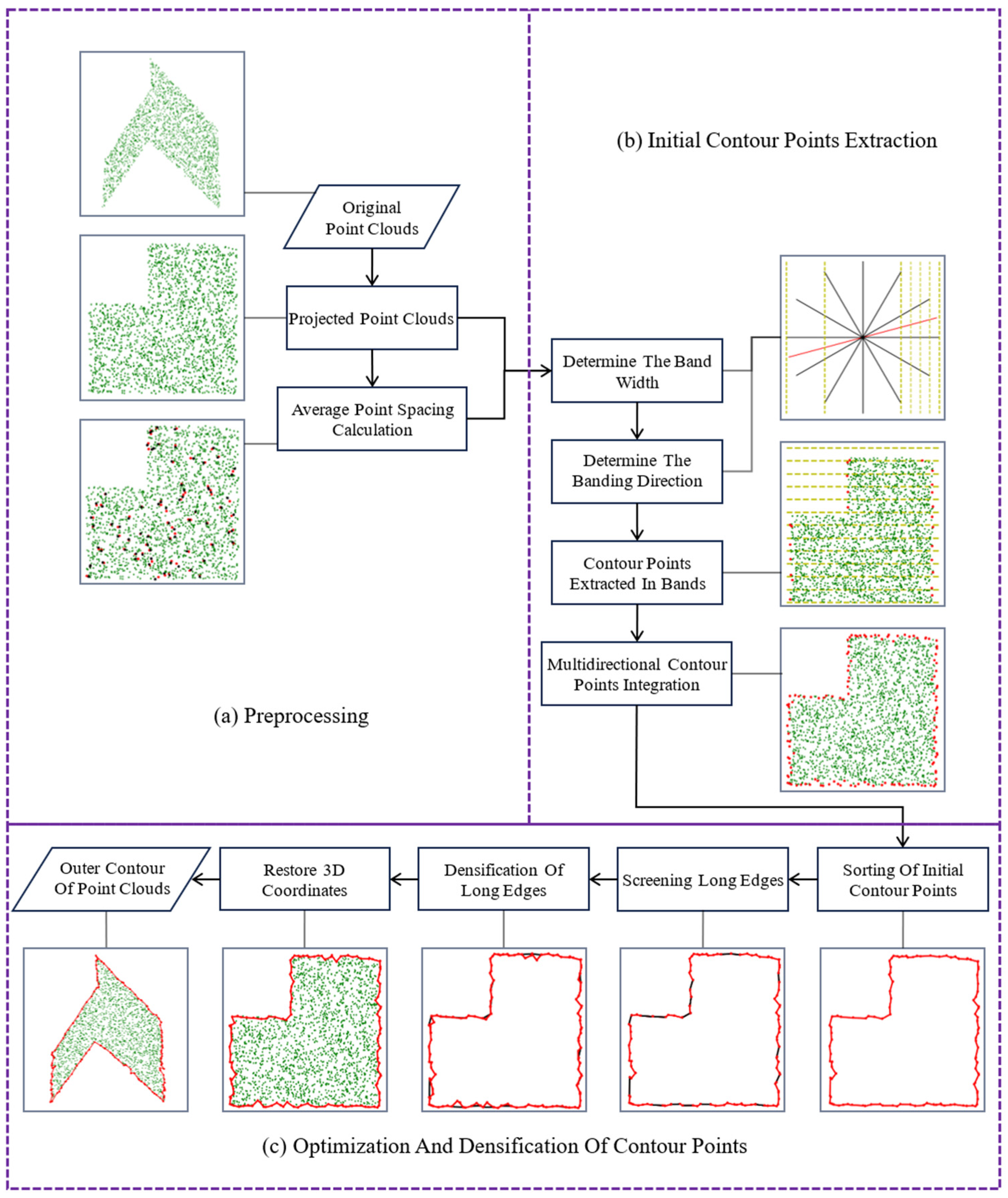
In this study, the proposed point cloud outer contour extraction algorithm based on multidirectional bands was mainly divided into three stages: data preprocessing, initial contour point extraction, and contour point densification and optimization. In the preprocessing stage, the average point spacing was calculated mainly for the following effective determination of the band width and banding direction; secondly, in the initial contour point extraction stage, the contour points were determined by single-direction banding, multidirectional banding extraction and result integration. In the process of single-direction banding extraction, the points in each band were vertically projected onto the central axis of the band, and the two points corresponding to the two farthest projection points on the central axis were determined to be contour points in the band; by changing the banding direction, contour points belonging to different banding directions were repeatedly extracted; finally, all contour points were integrated to obtain the initial contour points. Thirdly, the contour point densification and optimization stage specifically included three steps: initial contour point sorting, long edge determination, and long edge densification. On the basis of the determination of the initial edge segment, the contour points were sorted according to the principle of connecting the nearest point in the forward direction; the edge with the length that was greater than the length threshold was screened out and identified as a long edge; by selecting the noninitial contour point closest to the midpoint of the long edge in the neighborhood of the long edge, the long edge was iteratively densified until the length of each edge on the contour line met the length threshold, and finally a closed building roof outer contour line with the complete expression of the boundary structure was obtained. A flowchart of this algorithm is shown in Figure 1.
2.1. Point Clouds Outer Contour Extraction Based on Banding
2.1.1. Contour Points Extraction Based on Single-Direction Banding
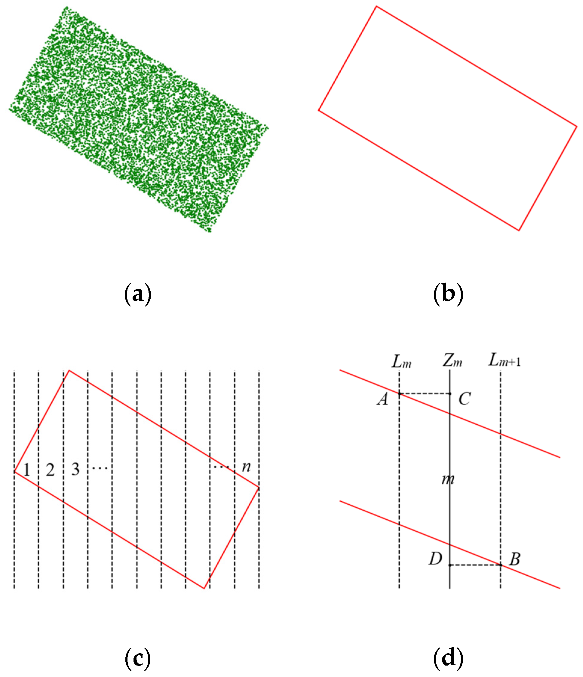
Three-dimensional point clouds on the roof of a building are projected onto a two-dimensional plane. If the point clouds are dense enough, the projected point clouds of the building roof can be approximated as a polygon composed of discrete points. As shown in Figure 2a, after the three-dimensional roof point clouds were projected onto a two-dimensional plane, the contour of the two-dimensional point set could approximate a polygon, as shown in Figure 2b. If the point clouds were dense enough and the contour points could be arranged continuously on the contour line, the edges of the polygon were composed of contour points arranged continuously. For any point cloud whose number was greater than 1, all of the points contained in it were vertically projected to a straight line in any direction, and the original points corresponding to the two farthest projection points were the two edge points of the point cloud, that is, the outer contour points. In order to extract the continuous contour points of the point cloud, the point cloud can be divided into n bands with the same width in any direction. Here, the division along the X-axis direction was taken as an example. As shown in Figure 2c, the smaller the band width, the greater the number of bands n. All points in each band were vertically projected onto the central axis in the current band, and the points corresponding to the two farthest projection points on the central axis were marked as contour points. By integrating the contour points in all bands, the coherent contour points of the point cloud in this band could be obtained. The process is specifically described as follows:
- For any band m, as shown in Figure 2d, m∈1, 2, …, n; Lm and Lm+1 are the left and right banding boundaries of the m-th band, respectively; and Zm is the central axis in the m-th band;
- All points in the m-th band are perpendicularly projected onto the central axis, Zm, to obtain a point set of the projected points, which is denoted as Pm;
- The two points with the farthest distance in Pm are marked as C and D, respectively, and the two points A and B in the m-th band corresponding to the two points C and D are marked as contour points belonging to the m-th band;
- All bands of the point cloud in this area are traversed, the above steps are repeated for each band, all extracted contour points in each band are added to the contour point set Q, and all contour points extracted from the point cloud in this area under single-direction banding are finally obtained.
2.1.2. Determination of Band Width
In the process of extracting contour points by banding, the band width, W, is a direct factor in the determination of the density of contour points. In case of a too small band width, there will be no points in some bands or the farthest two points projected on the central axis may be internal points. If the band width is too large, however, the extracted contour points will be too sparse, and, as a result, the roof contour structure will not be expressed comprehensively enough. In the process of point cloud data acquisition, the point spacing will vary due to the differences in the data acquisition equipment, flight heights, scanning modes, weather environments, and surface reflectivities [36,37,38,39]. Therefore, a fixed band width is hardly applicable to different point cloud data. To reduce the sensitivity of the algorithm to point spacing and improve the adaptability of the algorithm, the multiple of the average point spacing of the projection points was taken as the band width in this study.
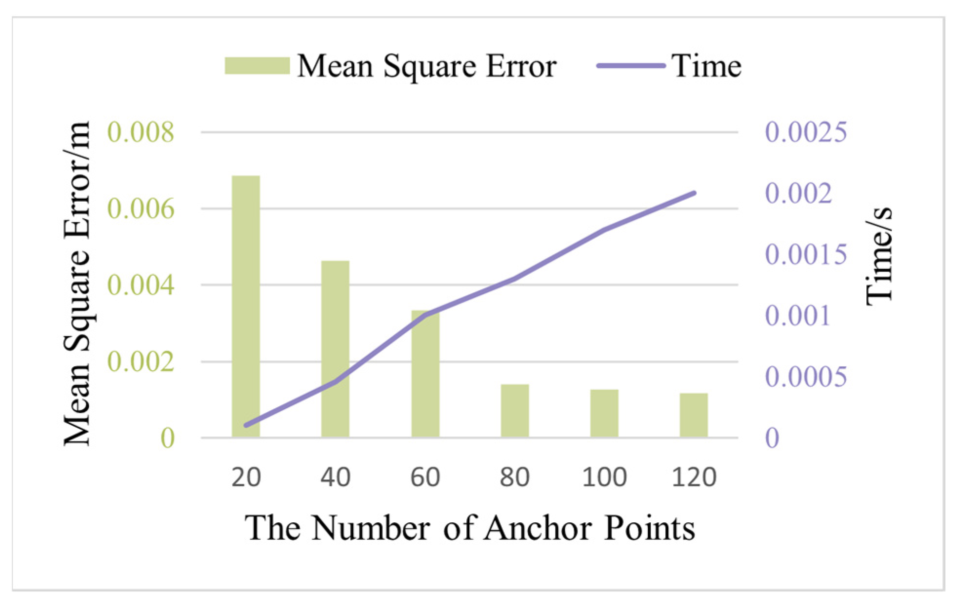
For the calculation of the average point spacing, to improve the efficiency when calculating, a kd-tree (k-dimensional tree) data structure was used to store the projected point clouds. Then, k points were randomly selected from the projection points as anchor points, the point nearest to the anchor points was determined using the nearest neighbor search method, and the average horizontal distance between all anchor points and their nearest points was taken as the average point spacing of point clouds.
where d is the average point spacing, k stands for the number of anchor points selected, and ei represents the horizontal distance between the i-th anchor point and its nearest point.
The larger the number of anchor points, k, the more stable the average point spacing is but the longer time it takes. Considering the above two factors, it is necessary to determine an appropriate k value. Figure 3 shows the operation’s results at k = 20, 40, 60, 80, 100, and 120, respectively. For each k value, k anchor points were randomly taken 20 times, and the average of the nearest point spacing of all of the anchor points was taken as the true value. Then, the Mean Square Error (MSE) of the point spacing and the average of the time consumed at each k value were calculated. It can be seen that the mean square error gradually declined with the increase in the number of anchor points, and the decrease tended to be gentle at k = 80, but the running time still increased stably, so k = 80 was set considering both efficiency and algorithm stability.
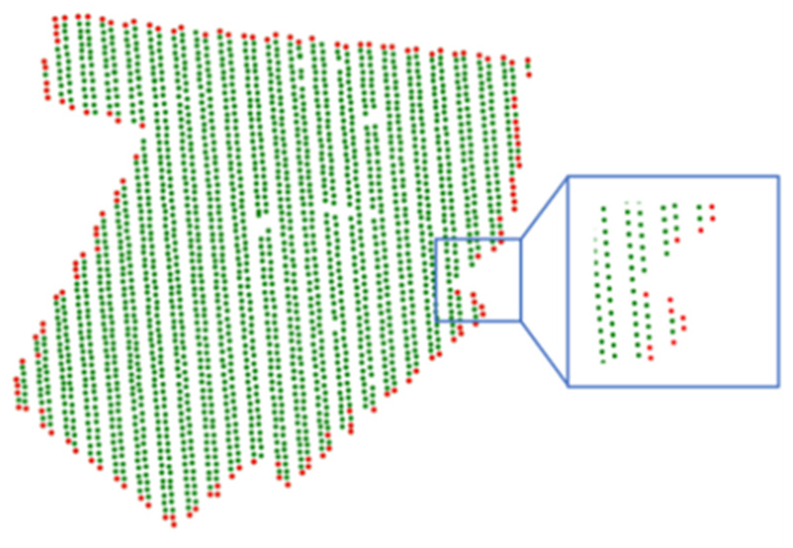
For the determination of multiples, after obtaining the average point spacing of the point cloud data, the multiple of the average point spacing was adopted as the band width, namely, W = N × d, where N is the multiple. Given a point cloud dataset, when W = 2d (i.e., the twice average point spacing was taken as the band width), the contour point extraction results for the point cloud are displayed in Figure 4a. The yellow, dotted line is the banding boundary along the direction of the Y-axis, green and blue points are noncontour points of different bands, and red points are contour points extracted at a band width W = 2d under single-direction banding. It can be observed from the figure that many internal points in the extraction results were marked as contour points, and the extracted contour points were irregular and distant from the actual contour line, so the band width should be appropriately adjusted.
To determine the optimal parameter value for multiple N, the contour point extraction results under single-direction banding conditions and N = 4, 6, 8, and 10 are listed in Table 1. Therein, Fm is the total number of extracted contour points; Fn represents the number of internal points misclassified as contour points; and F is the misclassification rate, specifically as seen in Equation (2). As the band width gradually increased, the total number of contour points and the number of misclassified points gradually declined. The misclassification rate peaked at N = 8, that is, the best contour points could be extracted when W = 8d in the case of single-direction banding, as shown in Figure 4b.
2.1.3. Determination of Banding Direction
In addition to the band width, the quality of the extracted contour points under single-direction banding conditions was also affected by both the banding direction and the shape of the original point cloud, which mainly manifested in the following two cases:
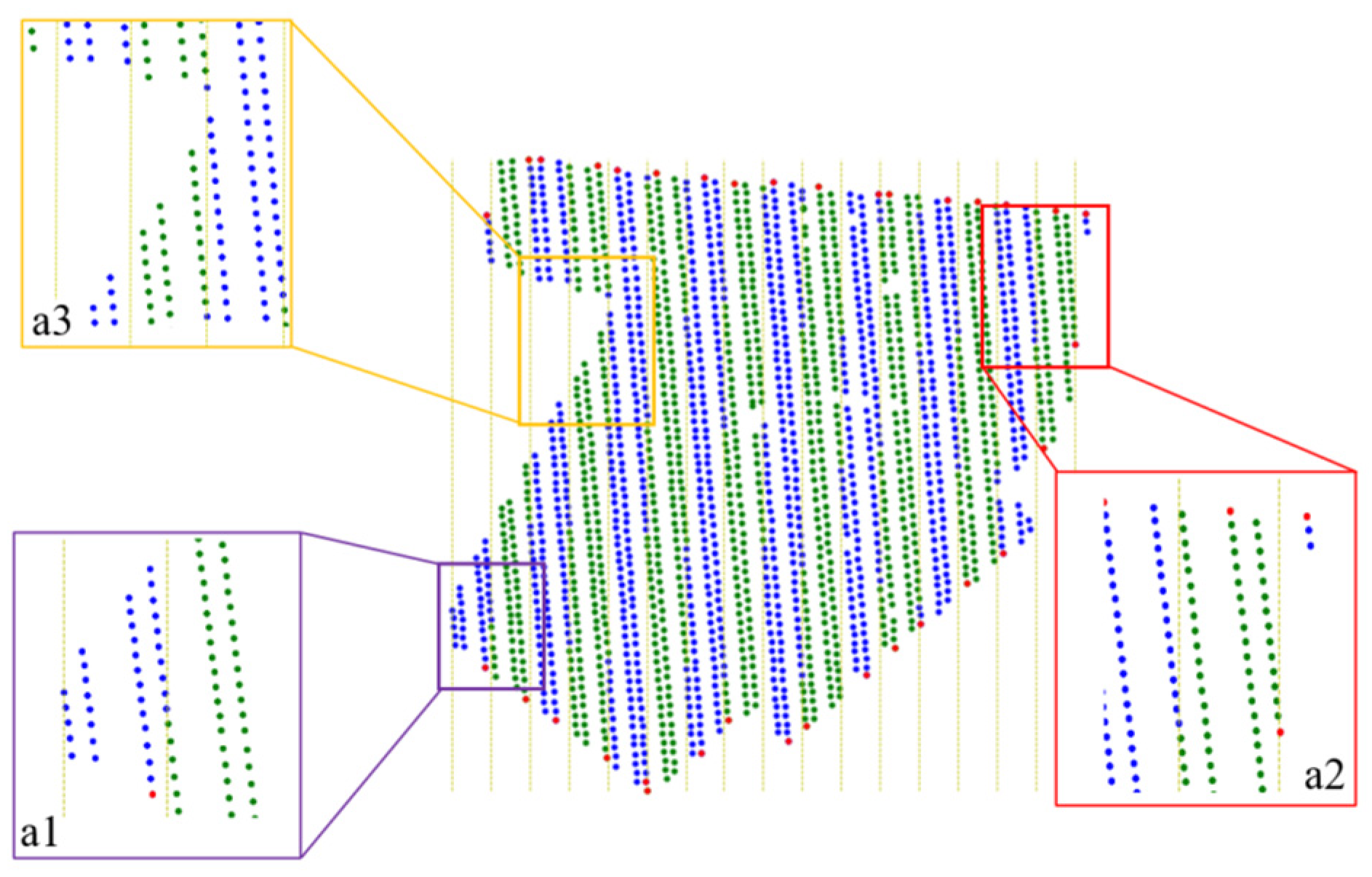
- When a contour line of the original point cloud is perpendicular or nearly perpendicular to the banding direction, if all points on the contour line exist in a band, and only two points, at most, in the whole band can be marked as contour points, some contour points will be missed, which results in too few contour points on the contour line approximately perpendicular to the banding direction, as shown in areas a1 and a2 in Figure 5;
- Given the local concave contour of the original point cloud, when the concave area is located in the middle of a single band after banding, the farthest distance between the projected points is generated by projecting the points located on both sides, which will lead to a wide range of missing results in the contour point extraction of the concave area under single-direction banding conditions, as shown in area a3 in Figure 5.
To obtain a more complete number of contour points, therefore, the abovementioned two problems were solved with multidirectional banding, which can avoid the missed extraction or large-scale omission of contour points.
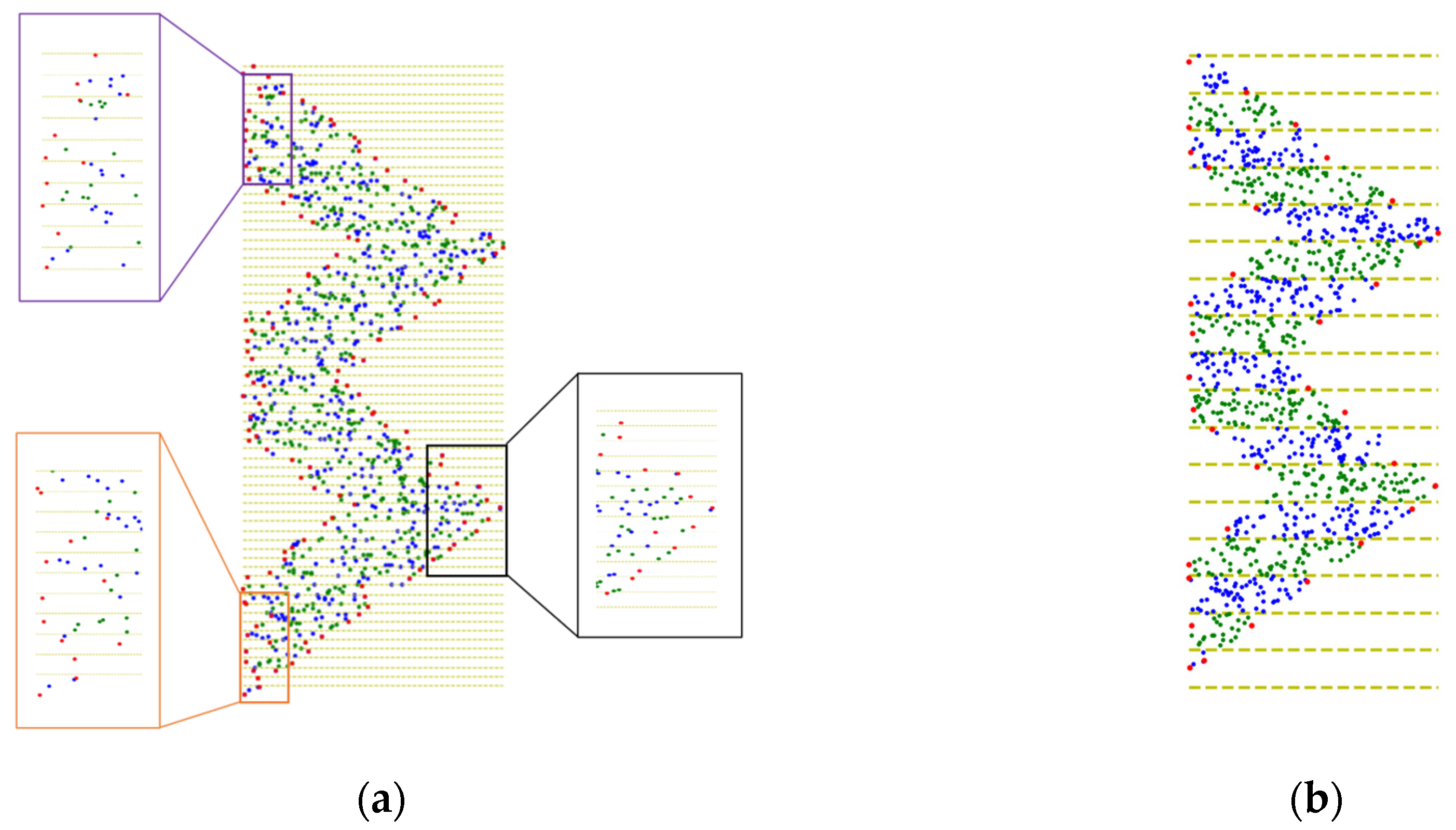
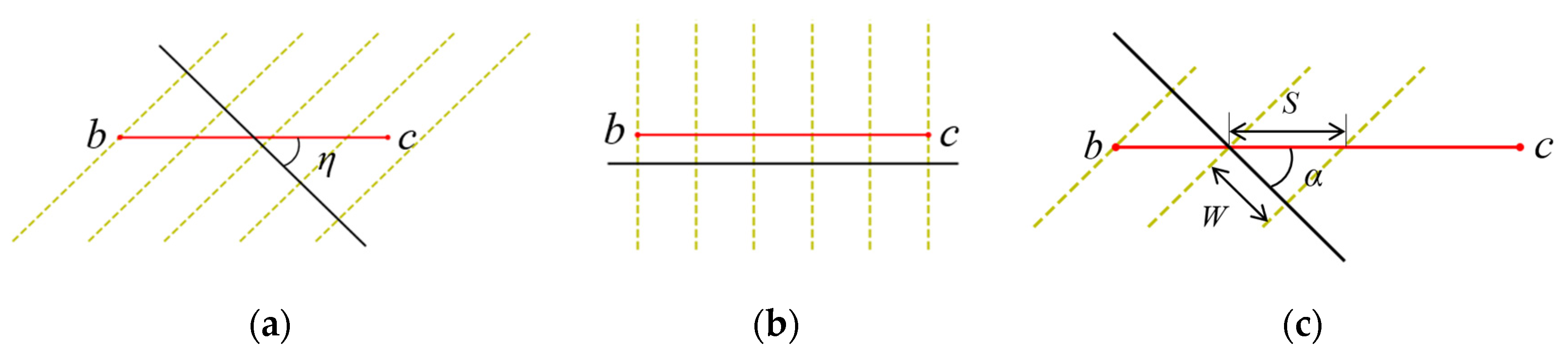
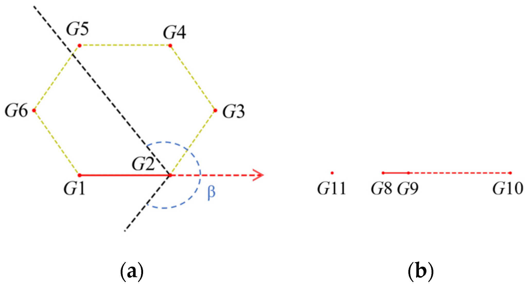
To ensure the stronger robustness of the multidirectional banding extraction algorithm, multiple banding directions were designated by means of 360° equal division; meanwhile, to ensure the more coherent contour points extracted from the point clouds, multidirectional banding aimed to divide each contour line into multiple bands as much as possible. The number of bands into which a contour line of fixed length could be divided depended on the size of the angle between the contour line direction and the banding direction. As shown in Figure 6, the red line segment, Lb,c, is an any contour line with a known length and direction; the direction of the black line represents the banding direction; and the yellow, dotted line is the banding boundary. In Figure 6a, the angle between the banding direction and the contour line direction is η, and the contour line is totally divided, in total, into 4 bands in this case. When η = 0°, the contour line is divided into a total of 5 bands, as shown in Figure 6b. Thus, it can be understood that if the angle η is reduced under a fixed band width, the contour line can be divided into more bands, i.e., the smaller the angle η, the greater the density of the extracted contour points on the contour line. On the contrary, the greater the angle η, the smaller the density of the extracted contour points, and the larger the spacing between adjacent contour points.
For multidirectional banding, the contour line Lb,c can constitute multiple included angles η with different banding directions. According to Table 2, the range of η is constant at 0–90°, and the smallest included angle η therein is recorded as α. At a fixed band width W, as shown in Figure 6c, the relationship of the distance, S, between adjacent points with the included angle, α, can be expressed using Equation (3), and it can be seen that S increases with the growth in α within the range of 0–90°. Hence, the theoretical value of the maximum distance, Smax, between adjacent contour points extracted from an any single-direction band under multidirectional banding conditions within the value range of α can be solved via Equation (3). This value is the allowable maximum distance between adjacent contour points on the contour line extracted through multidirectional banding. If the distance between adjacent contour points in the extraction result is greater than Smax, this means that no contour points were extracted in this area under all banding direction conditions, and there is an extraction loophole.
Taking six-directional banding as an example, as shown in Figure 7, the range of the angle α between an any banding direction and the contour line is α∈[0°,15°]. When W = 8d and α = 15°, the maximum distance between adjacent contour points in the six-directional bands can, therefore, be solved as Smax ≈ 8.28d, according to Equation (3), i.e., the allowable maximum distance between adjacent contour points on the contour line under six-directional banding conditions is 8.28d. This value can be applied to identify the long edge generated in the case of contour point extraction loopholes.
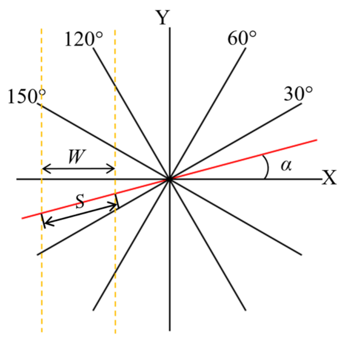
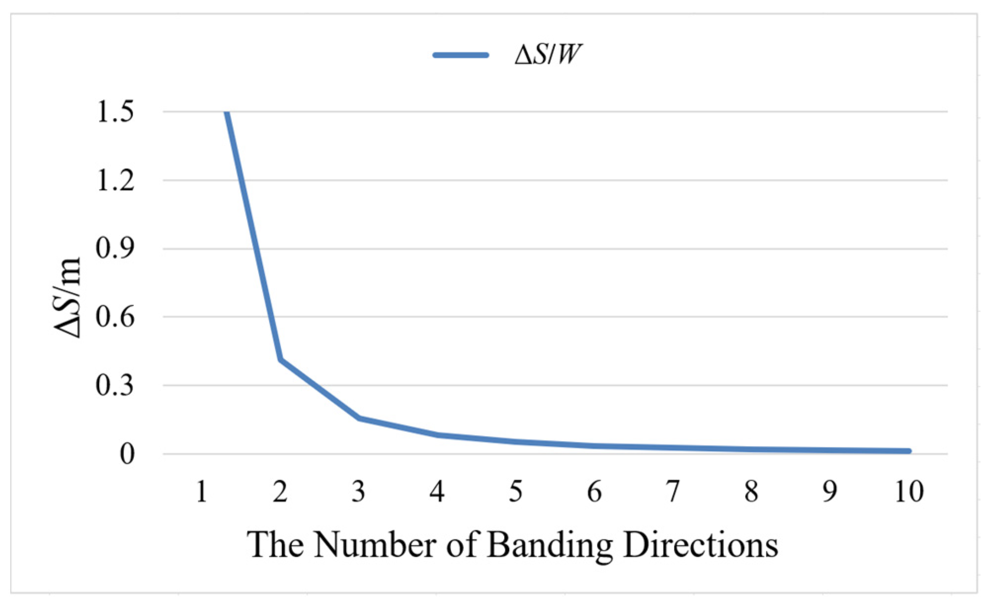
Since the value of S determines the coherence of the contour points on the contour line and it can be known from Equation (3) that S is always greater than or equal to W, the difference in the allowable maximum distance between adjacent contour points and the band width under the different number of banding directions were calculated using Equation (4) and recorded as ΔS, the unit of which is a single band width. The smaller the ΔS, the more coherent the contour points. When the number of banding directions is N0 = 1, 2, 3, …, 10, that is, from a single direction to ten directions, it can be observed in Figure 8 that ΔS sharply declines with the increase in the number of banding directions, and it tends to change gently if the number of banding directions is greater than 6. When contour points are extracted using the multidirectional banding method, since the same point may exist in multiple different bands, the same contour point may be extracted multiple times, and the misclassified points extracted in different bands will accumulate in the initial contour points, making it inappropriate to use too many banding directions. To ensure that the contour points extracted with multidirectional banding are relatively high in quality and possess enough density, it is necessary to decrease the interval of the largest distance between adjacent contour points on the contour line as much as possible while reducing the number of banding directions, so it is appropriate to set N0 to 5–7.
When N0 = 6, six directions—0°, 30°, 60°, 90°, 120°, and 150°—are selected, whereby 0° and 90° are the X-axis direction and the Y-axis direction, respectively. The contour points extracted based on six-directional banding are shown in Figure 9. Compared with the contour extraction results obtained by single-direction banding, as shown in Figure 5, the contour points extracted by the former have better coherence and can express the contour of the point cloud well. However, some contour points were still not extracted in individual, small-scale local concave areas, making it necessary to locally densify and optimize the initial contour points.
2.2. Densification and Optimization of Initial Contour Points
In this study, the extracted contour points were connected to construct a complete contour line, so the density of the contour points determines the fitting degree of the contour line. For local feature areas with missing extraction of contour points, such as concave areas with feature inflection points, if the distance between connected contour points is greater than the maximum tolerable distance, Smax, it is considered that there will be some deviation between the fitting edge and the real edge. Hence, the contour points in this area should be densified and optimized using the nearest neighbor search method.
2.2.1. Sorting of Contour Points
The initial contour points extracted by six-directional banding are disordered, without topological relationships between points. In order to facilitate the subsequent densification of contour points, it is necessary to sort the initial contour points first and establish the topological relationships between the points so that the initial contour points form an initial contour line that is connected end to end. It is assumed that the initial contour point set obtained by six-directional banding is G, and the contour points contained therein are shown in Figure 10a. The specific implementation process of contour point sorting is as follows:
- First, j = 0 is set, a starting point for the contour line search is randomly selected from the initial contour point set G and recorded as Gj, and it serves as the current searching point and is removed from the point set G;
- The point nearest to the current searching point Gj is found in the residual contour points of the point set G and recorded as Gj+1. Gj+1 is then added into the contour line and connected to Gj. The direction from Gj to Gj+1 is the positive direction of the searching line segment, as indicated by the direction of the red, dotted line in Figure 10a;
- Then, j = j+1 is set, and the current searching point Gj is updated, i.e., the point newly added to the contour line is regarded as the current searching point and removed from the point set G;
- Steps (2)–(3) are repeated until the point set Gj is empty, and the point finally added to the contour line is connected to the starting point to obtain a closed contour line.
If the initial contour points are connected or sorted only by the distance, there will be a situation in which the points are selected in the opposite direction to that of the current searching line segment. As shown in Figure 10b, the line segment connected by G8 and G9 is the current searching line segment, and G9 is the current searching point. Because the distance from G11 to G9 is shorter than that from G10 to G9, G9 and G11 will be connected. To avoid the backward connection, the following constraint condition is added to the search process of the above Step (2), that is, a β-degree sector area formed by taking the current searching point as the center and the extension line on the positive side of the current searching line segment as the central axis is taken as the searching area, and the point Gj+1 closest to the current searching point Gj is found in the searching area. Through repeated experiments, β = 240 was set in this study.
2.2.2. Optimization and Densification of Long Edges
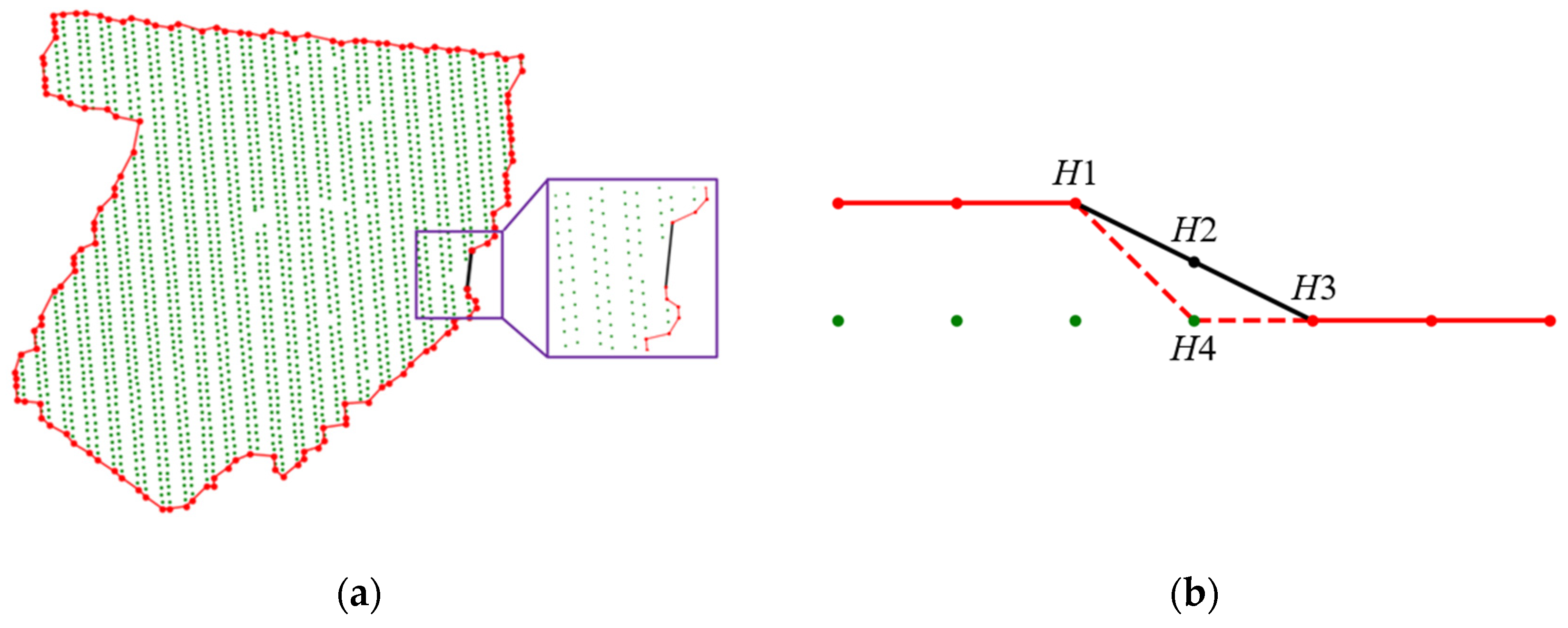
Ideally, for the point cloud data of a building roof with uniform density and complete boundary collection, there is no case in which the edge points are occluded in the process of extracting contour points by banding, all edge points can be extracted effectively, and the length of each line segment on the initial contour line obtained should be less than or equal to the maximum distance Smax = 8.28d, which is obtained using Equation (3). However, for individual concave areas where bands in all directions will be occluded, there will be edge segments with lengths greater than the maximum distance, Smax. In this study, such edge segments were referred to as long edges, which were subjected to further densification and optimization.
Because of the uneven density of the point cloud data, judging whether each edge on the contour line is a long edge strictly on the basis of the maximum distance Smax = 8.28d is not, in fact, applicable to real point cloud data. To ensure the accuracy of long edge screening, therefore, the threshold, T, for judging a long edge should be appropriately increased, taken as T = 10d here. As shown in Figure 11a, the red line is an edge with a length smaller than the threshold, T, and the black line is a long edge.
To express the boundary contour of point clouds completely, it is necessary to densify and optimize the long edge. New contour points are extracted in the neighborhood of the long edge and inserted into the long edge so that it becomes several short edges with a length less than the threshold, T. As shown in Figure 11b, LH1,H3 is a long edge with a length greater than the threshold, T; the midpoint, H2, of line segment LH1,H3 was taken; the point H4 closest to H2 was searched from the noninitial contour point set; and H1 and H3 were connected to H4 to form two new contour edges: LH1,H4 and LH4,H3, respectively. If the lengths of both of the above newly generated contour edges are less than the threshold, T, the densification of long edge LH1,H3 is completed; if a long edge is longer than the threshold, T, exists in the generated contour edges, the above process is repeated, the new long edges are densified once again, and no contour points will be inserted when the lengths of all line segments constituting the contour line are less than the threshold T. At this point, the final outer contour line of the point clouds, extracted by multidirectional banding, is acquired. Since all points in the outer contour line come from the original 3D roof point clouds, the elevations of all contour points can be recovered according to the correspondence between the projected points and the original 3D points, thus acquiring the 3D outer contour line of the original point clouds.
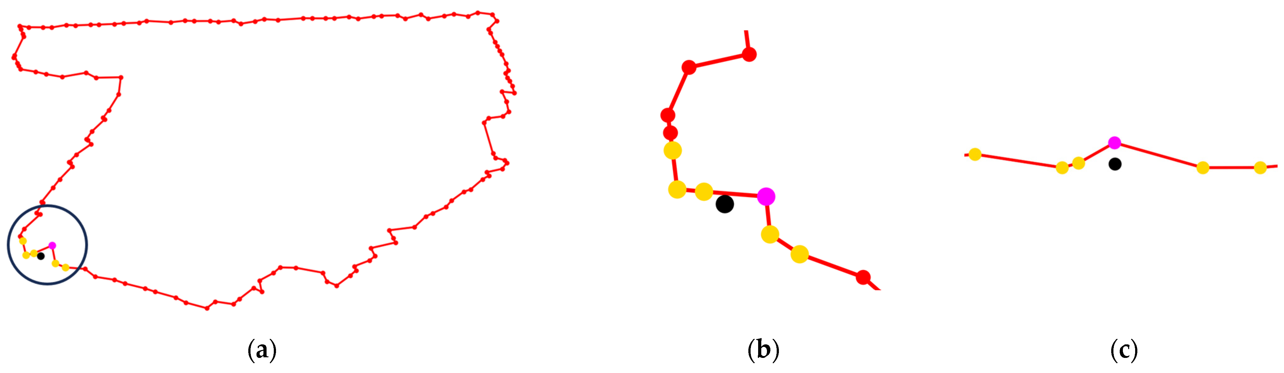
To avoid the existence of noise points in the contour line, such as the points of the parapet walls on the roof, which lead to the local elevation suddenly changing after the contour line is recovered into 3D, this paper adopted the local average elevation of the contour line to eliminate the potential noise points in the extracted contour points. As shown in Figure 12, the purple point is a randomly selected contour point, the yellow points are the five nearest contour points to the purple point in the 2D plane, and the coordinates of the black point are the mean value of the three-dimensional coordinates of the current five yellow points. If the elevation difference between the purple point and the black point is greater than 5d, then the current purple point is considered to be a noise point in the contour line, and it is removed from the contour line.
During the optimization of the long edges on the contour line, the threshold, T, can be reduced to acquire denser and more coherent contour points in order that the extracted outer contour of the point clouds fits better with the actual boundary of the point clouds. Figure 13a,b display the densification results of the initial contour points under T = 10d and T = 5d. Therein, the black, solid line is the long edge contained in the initial contour line, and the red, solid line represents the contour line after densification. It can be seen that the contour line extracted under T = 10d is relatively flat. When T = 5d, the concave area is expressed in a more detail by the contour line in Figure 13b yet accompanied by possible overfitting. The proposed algorithm can determine the fitting degree of the contour line by setting different thresholds, T, to acquire the building roof contour catering more to work needs.
3. Experiment Results and Analysis
3.1. Experimental Data
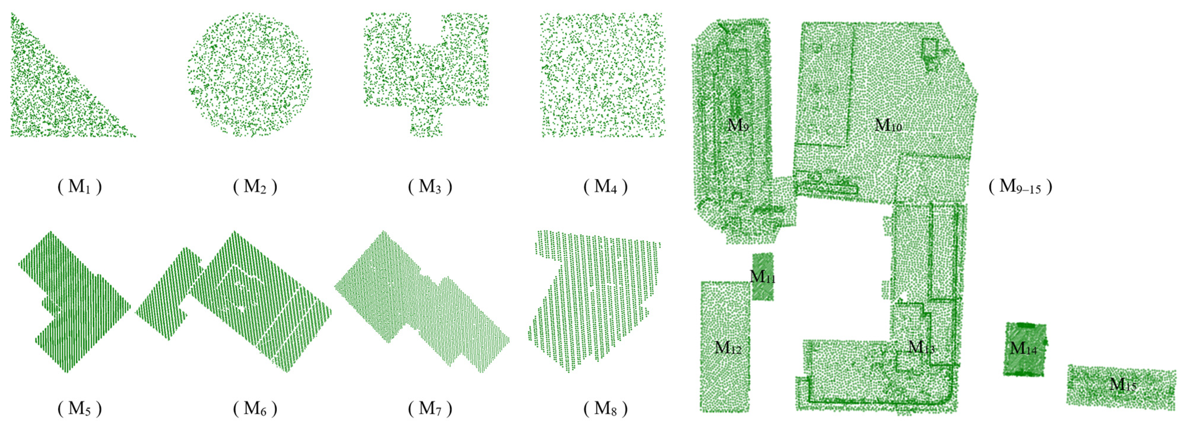
In this study, three groups of different types of point cloud data, as shown in Figure 14, were selected for the experiments, and they were recorded as datasets 1, 2, and 3. Dataset 1 displays a group of point clouds with uneven densities and different boundary structures acquired with the 3D entity model, which were used to simulate the point clouds with such boundary structures as acute angles, arcs, concave–convex, and right angles in reality, as indicated by M1–M4 in Figure 14. Dataset 2 and Dataset 3 were obtained from the Vaihingen dataset provided via the official website of the ISPRS, and the DublinCity dataset was provided by Reference [40]. The building roof point clouds in both datasets are accurately labeled. Dataset 2 exhibits the representative building roof point clouds chosen from the Vaihingen dataset, as expressed by M5–M8 in Figure 14. Compared with Dataset 1, the point clouds were distributed more evenly in Dataset 2, and the building roof displayed more complicated boundary structures; Dataset 3 presents the point clouds in Dublin city areas chosen from the DublinCity dataset, and the regional point clouds containing 7 buildings (M9–M15) were selected in the experiment. The average point spacings for M1–M15, calculated as per Equation (1), are listed in Table 3.
3.2. Results and Analysis
3.2.1. Comparative Analysis of Extraction Results under Different T Values
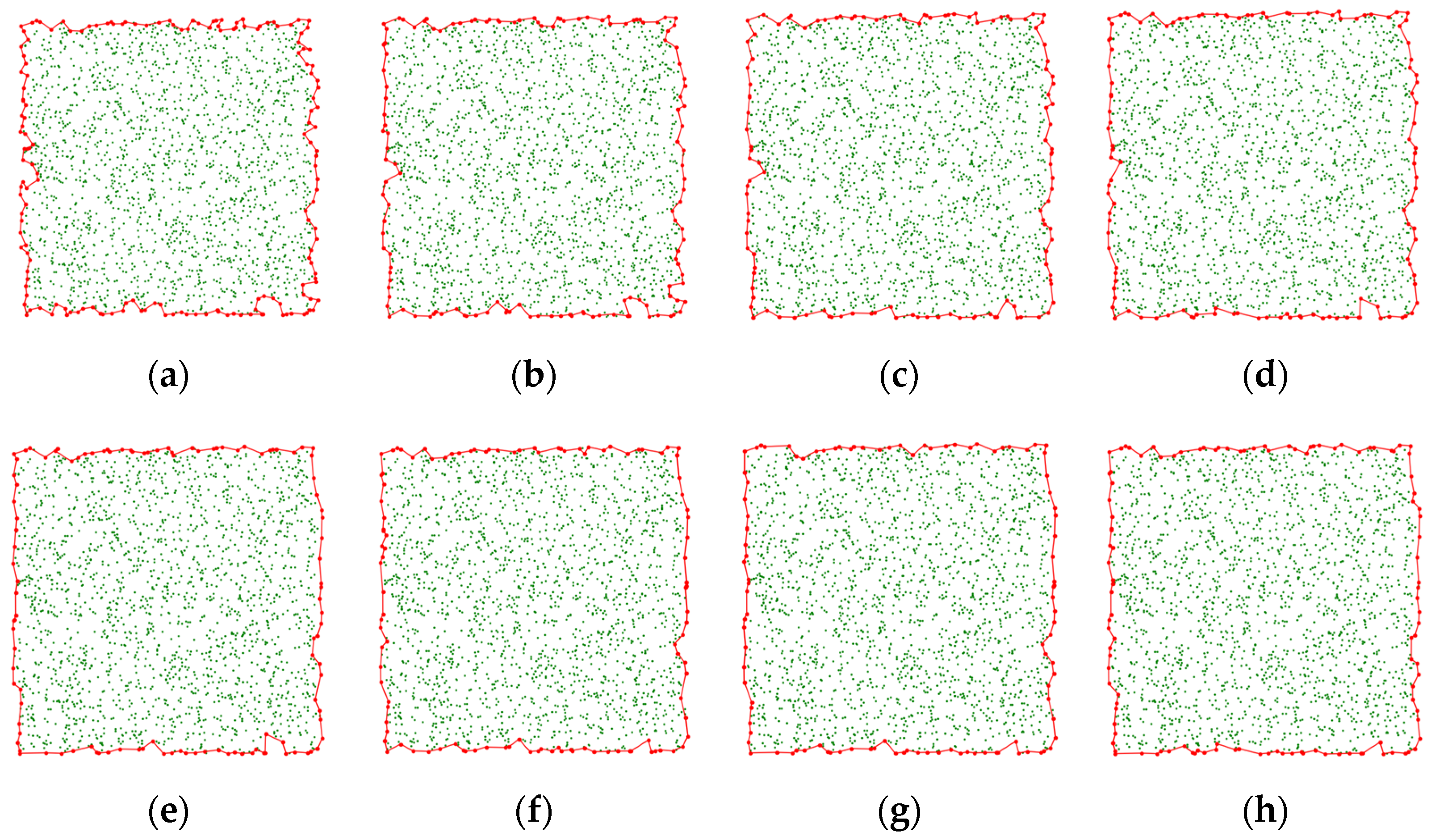
To analyze the influence of different T values on the contour extraction results, different T values were set to extract the contour of point cloud M4, which has uneven density and a large average point spacing, and the extraction results are shown in Figure 15.
When T = 4d, as shown in Figure 15a, all long edges longer than 4d in the initial contour line were densified under the small densification threshold, T, which led to the irregularity of the extracted contour line, a great difference from the actual boundary shape, and the too refined expression of the boundary shape for the original point clouds. When T = 11d, as shown in Figure 15h, few long edges were screened out from the initial contour line, which, as a whole, was relatively flat and similar to the actual boundary shape. Since contour points were extracted by six-directional banding and the maximum tolerable distance between adjacent contour points was Smax ≈ 8.28d, only a few long edges could be screened when T ≥ S: T = 9d, T = 10d, and T = 11d. Hence, the extracted contour lines were all relatively resembled the actual boundary shape.
3.2.2. Qualitative Analysis of Contour Line Extraction Results
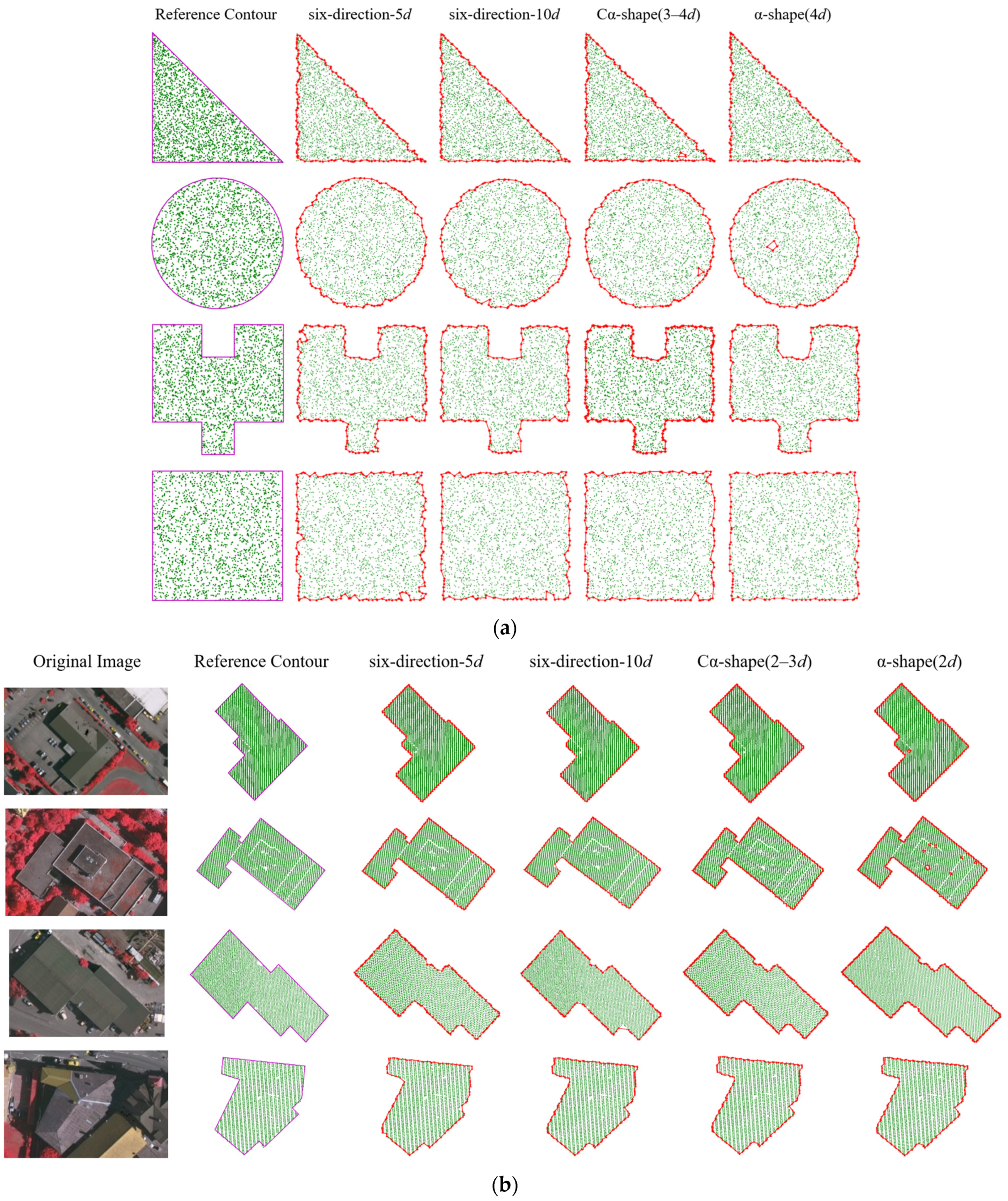
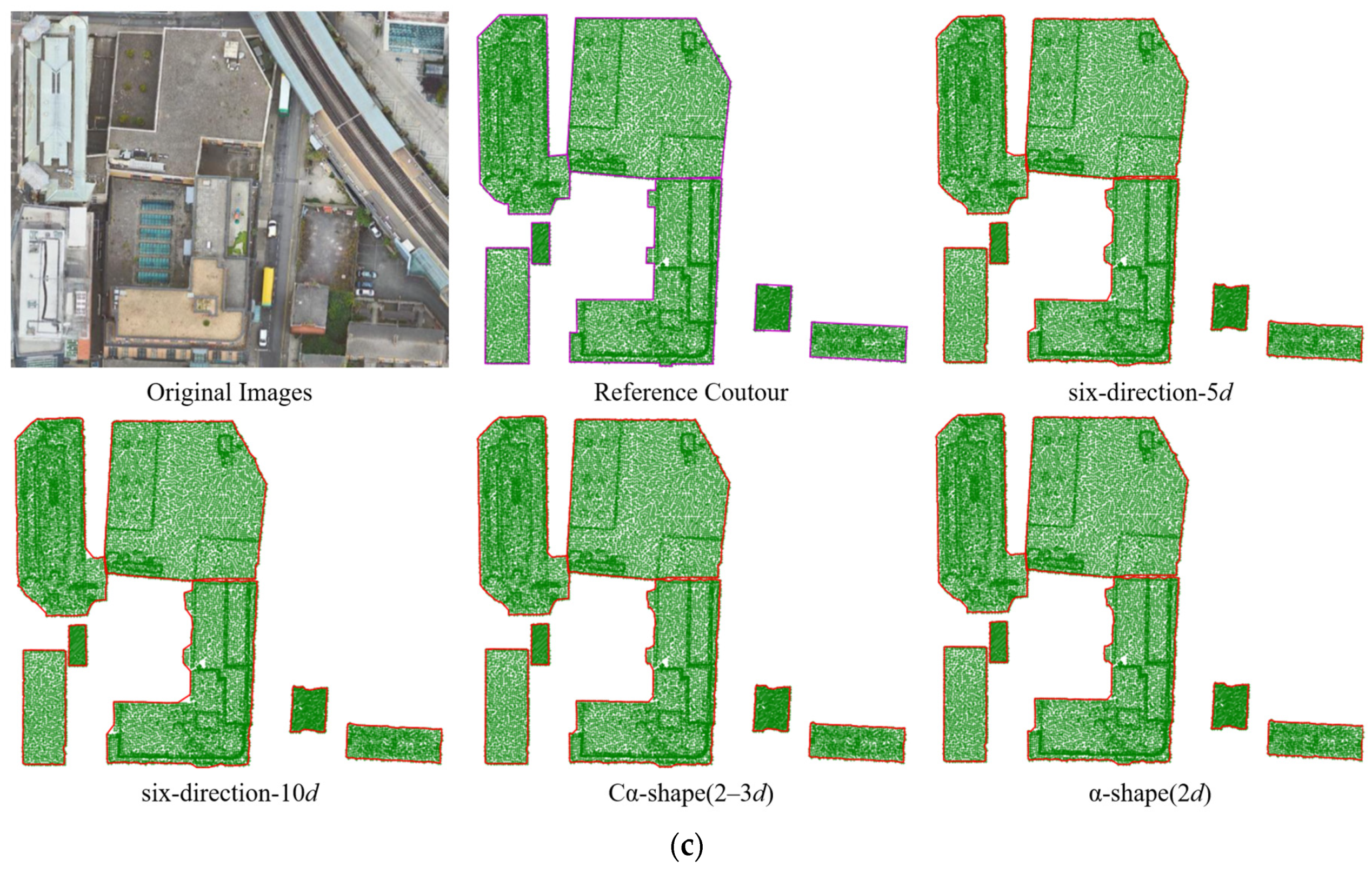
To verify the effectiveness of the algorithm proposed in this study, it was compared with the alpha shapes method and variable-radius alpha shapes method, and the contour line extraction results obtained with different algorithms are displayed in Figure 16. In the proposed algorithm, N0 = 6, and a comparative analysis was performed for T = 5d and 10d, in which the six-directional banding methods under the densification thresholds of T = 5d and T = 10d were briefly recorded as six-direction-5d and six-direction-10d. Given the different changes in the point cloud density in each dataset, the parameter r in the alpha shapes method and variable-radius alpha shapes method should be changed. Therein, Cα-shape(2–3d) and Cα-shape(3–4d), respectively, represent the variable-radius alpha shapes method with a rolling ball radius of r = 2–3d and r = 3–4d; α-shape(2d) and α-shape(4d), respectively, denote the alpha shapes method under a rolling ball radius of r = 2d and r = 4d. The key parameters adopted in the different algorithms for each dataset are listed in Table 4.
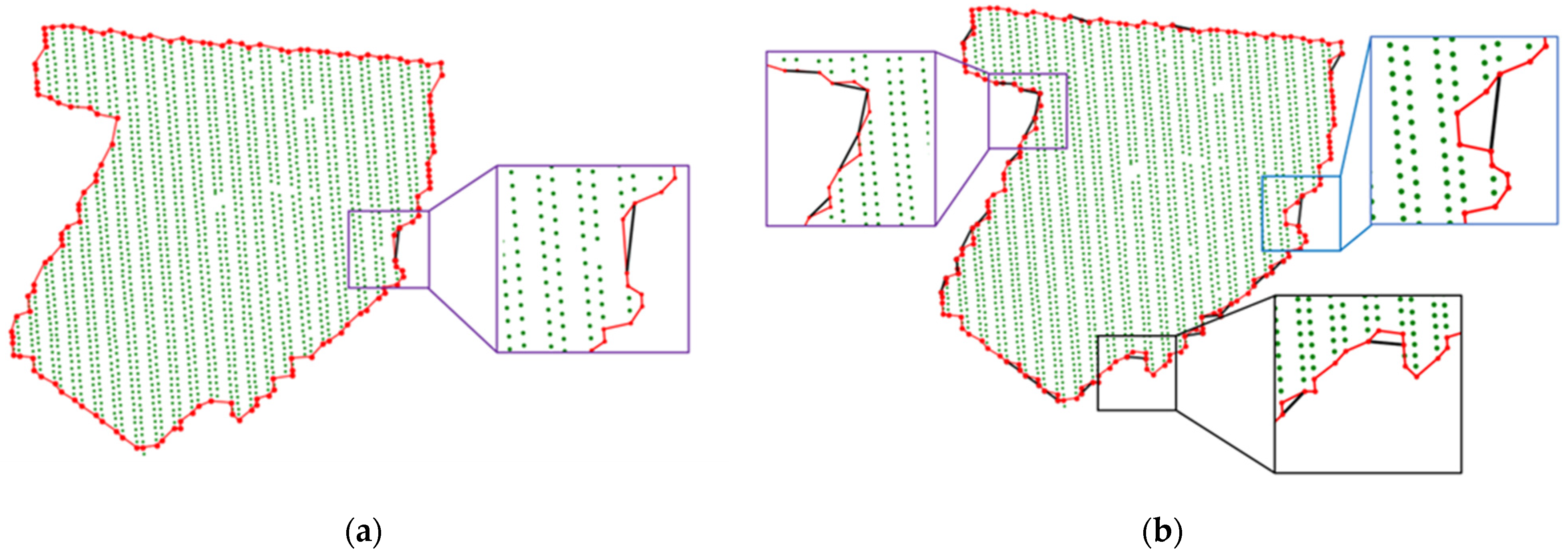
According to the contour extraction results of the different algorithms, as shown in Figure 16, in the case of great changes in the point cloud density among the different data, the parameter values for the alpha shapes method and variable-radius alpha shapes method should be changed to extract relatively complete contour lines. However, the proposed algorithm is capable of extracting relatively complete contour lines under a constant threshold without needing to change the parameter values. When contours are extracted using the variable-radius alpha shapes method, point clouds will be divided into auxiliary grids, the points belonging to the overall contour in the boundary grids are judged, and the rolling ball radius is appropriately and automatically reduced for the rough boundary grids. As a result, the hole boundary in the boundary grids is marked as a point cloud contour, as indicated by M2 in Figure 16a. In the contour extraction process using the α-shape(4d) method, the point cloud holes near the boundary are not extracted, but they will be extracted if the Cα-shape(3–4d) method is adopted. In the case of many holes inside the point cloud, all contour lines meeting the conditions will be extracted if the alpha shapes method is used, as expressed by M6 in Figure 16b. When the α-shape(2d) method is adopted, many internal hole boundaries will be marked as contour lines.
By analyzing the contour extraction results of the different algorithms from M1–M15, it can be seen that, in the case of minor cloud point density changes and no evident internal holes (e.g., M7, M8, M11, and M12), each algorithm can extract contour lines with favorable quality. For the point clouds with internal holes (like M6), the boundaries of internal holes will be extracted together during the point cloud contour extraction based on alpha shapes method, which results in the declining quality of the contour. For point clouds with holes in the boundary grids (like M2), the variable-radius alpha shapes method will also extract the boundaries of internal holes. However, the six-directional banding method is highly adaptable to hole-containing point clouds and can stably extract the outer contour of point clouds. As the density change in the point clouds increases, it is difficult when using the alpha shapes method and variable-radius alpha shapes method to determine an appropriate rolling ball radius; under a constant densification threshold, the six-directional banding method can still extract the outer contour of the point clouds, proving that the proposed algorithm adapts better to the point clouds with great density changes and internal holes, accompanied by easier setting of parameters.
3.2.3. Quantitative Analysis of Contour Line Extraction Results
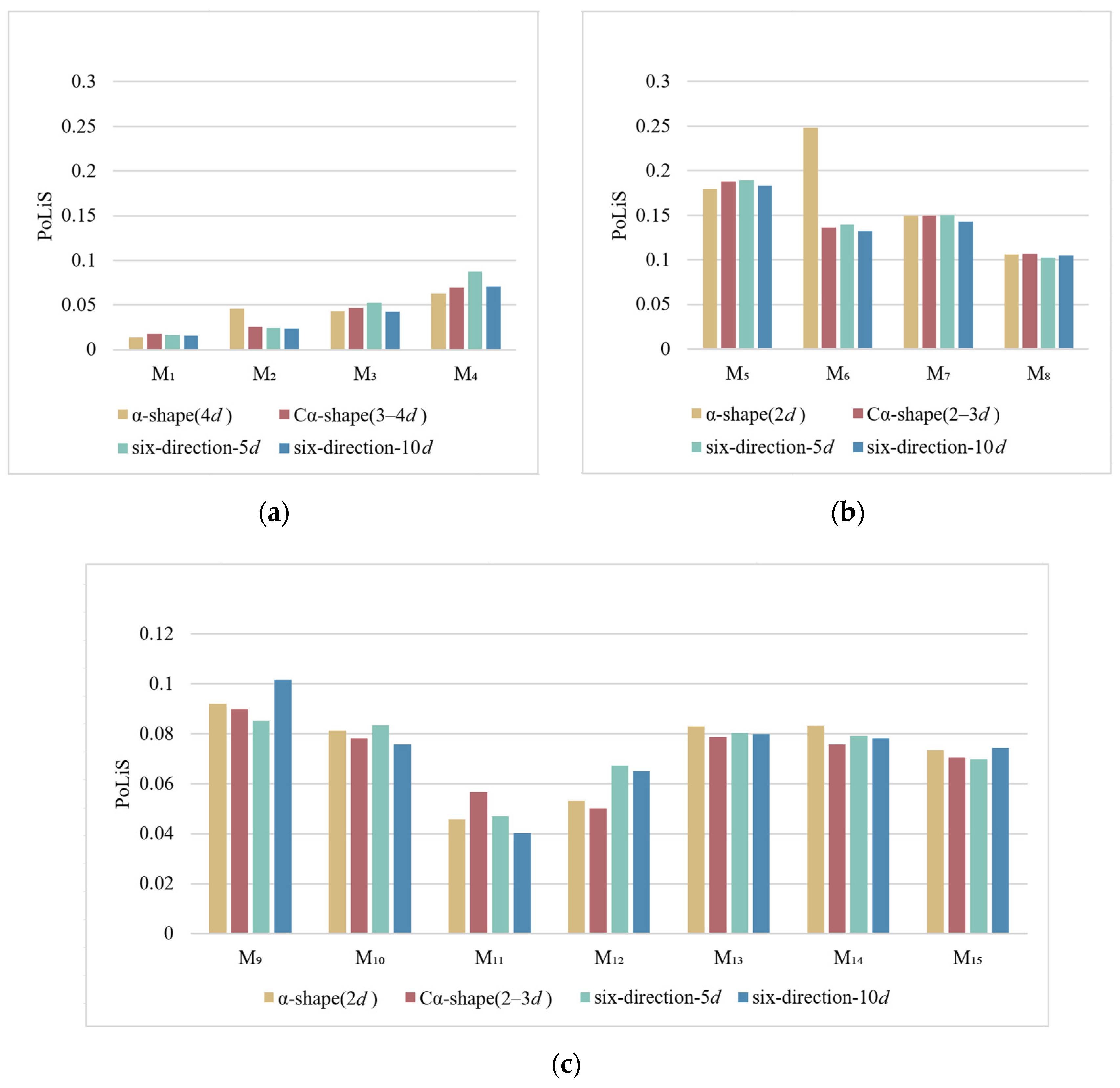
To quantitatively analyze the contour extraction results of the algorithm in this study, the accuracy of the results was analyzed using two indicators, namely, PoLiS measurement and Relative Area Error (RAE). PoLiS measurement is an index proposed by Avbelj et al. to judge the similarity between two polygons [41]. When one polygon has more vertices than the other, PoLiS measurement is superior to Hausdorff distance and chamfer distance. In this study, the similarity between the extracted contour polygon and the reference contour polygon was analyzed by PoLiS measurement, and the difference between the extracted area and the reference area was compared using RAE. The smaller the PoLiS measurement and RAE value, the higher the similarity, accuracy, and completeness of the extracted contour and the reference contour. The reference contour of Dataset 1 was provided by the original three-dimensional model. With reference to the shape of the building roof contours in high-resolution images, the reference contours of Datasets 2 and 3 were created by displaying the point clouds in Computer-Aided Drafting (CAD) software and drawing them by hand. The statistical PoLiS measurement results for the contour extraction of the three datasets using different algorithms are shown in Figure 17, and the formula for PoLiS is shown in Equation (5). The statistical results of the RAE value, calculated according to Equation (6), are listed in Table 5.
where A and B are two polygons; p and q are the number of points in polygons A and B, respectively; ai and bj are the points in polygons A and B, respectively; and i∈1, 2, …, p, and j∈1, 2, …, q.
where U is the polygonal area of the reference contour; ΔUi represents the difference between the polygonal area of the extracted contour and that of the reference contour.
As can be seen from Table 5, the RAE values of the point cloud contours extracted using the six-direction-10d method are the lowest, except for five groups of data—M2, M3, M12, M14, and M15—and the difference between the five groups of data with higher RAE values and the lowest values of the same group of data was less than 1%, indicating that the area extracted by the six-direction-10d algorithm was closer to the reference area. According to the PoLiS measurement, as shown in Figure 16, it can be seen that the PoLiS measurement of the extraction result of this algorithm was less affected by the local change in parameter values, and the overall PoLiS measurement was low, revealing that the parameters of this algorithm have relatively weak influences on the extraction result, and the extracted contour is more similar to the reference contour. Through the analysis of the RAE value and PoLiS measurement value, it can be seen that the contour extracted using the algorithm proposed in this study is complete and correct, and the algorithm is robust for different point cloud data, with easier setting of the parameters.
3.2.4. Analysis of Algorithm Running Efficiency
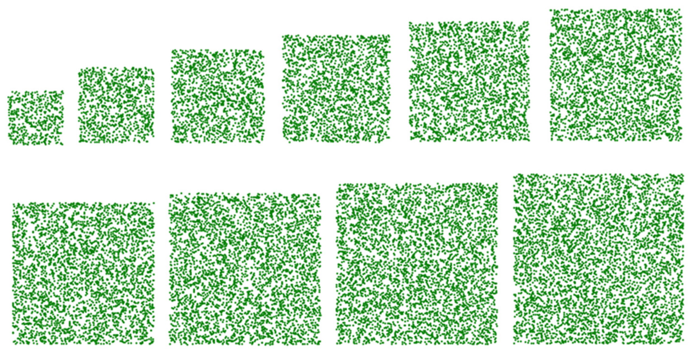
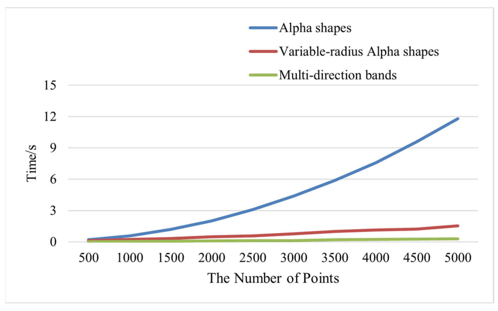
To prove the efficiency of the proposed algorithm, Dataset 4, consisting of simulated point clouds with the same shape, density, and density changes but different quantities, was artificially selected from the 3D entity model for the sake of the contour extraction experiment, as shown in Figure 18. The contour extraction was performed using the alpha shapes method, the variable-radius alpha shapes method, and the proposed algorithm, respectively. The running times for the three algorithms are shown in Figure 18.
It can be observed from Figure 19 that as the number of points continuously grows, the running time of the alpha shapes method rises sharply, indicating that the alpha shapes method is inapplicable to point cloud contour extraction with a large number of points. Since the variable-radius alpha shapes method uses adaptive-radius alpha shapes for the points in the virtual grid, its running time is shorter compared to the alpha shapes method, but as the number of points continues to grow, it will maintain an exponential growth trend. With the increase in the number of points, the running time needed by the proposed algorithm basically shows a linear rising trend, and the time consumed is always the shortest when the contour extraction is performed on point clouds containing different numbers of points.
4. Discussion
The uneven density and internal holes of point cloud data are important factors that affect the accuracy of contour lines extracted using existing algorithms. In this paper, we used multidirectional bands to weaken the influence of the quality of the original point cloud data on the contour line extraction results. Compared with the existing algorithms, the algorithm has the following characteristics: it needs fewer parameters and the parameters are adaptive, and it is more robust for point clouds with different densities; compared with the existing point-by-point judgment algorithm, this method takes each band as a unit to improve the operating efficiency of the algorithm; on the one hand, multidirectional banding avoids the missing extraction of contour points in single-direction banding and ensures the integrity of contour extraction; on the other hand, it makes the algorithm more robust for point cloud data with different shapes and densities. By analyzing a large quantity of data, the number of banding directions is determined as N0 = 5–7, and a band width of W = 8d (8-fold average point spacing) is a relatively stable parameter range. The proposed algorithm was used to perform contour extraction experiments on building roof point cloud data provided in two opensource datasets. The experimental results show that the proposed algorithm is more adaptable to point clouds with large density variations and can eliminate the interference of holes in point clouds with the extraction results. However, it is not ideal to use this algorithm to determine whether it is a long edge that needs to be densified and optimized only using a single edge length constraint. Influenced by the point cloud data acquisition method and the building structure, a single length constraint will lead to the over-refining of some regular edges, which will result in irregularity. Hence, the screening conditions for long edges will be further added to strictly screen out those long edges needing densification, reserve the originally flat contour lines in the initial contour lines, and densify the contour lines with an incomplete expression of boundary structures to further enhance the accuracy of the contour line extraction.
5. Conclusions
In this study, an algorithm for extracting the outer contour of building roof point clouds based on multidirectional banding was proposed. This method divides a point cloud into multidirectional bands, and each band is a processing unit. The points in each band are projected on the central axis of the band, and the contour points are extracted by determining the farthest distance point on the central axis. In the comparison of the contour line extraction results of the proposed algorithm with those of state-of-the-art contour line extraction algorithms, the strengths and weaknesses of the proposed algorithm were objectively analyzed, providing a new algorithm for efficiently extracting the contour of building point clouds.
Author Contributions
J.W. and D.Z. contributed to the design of the methodology and the validation of the experimental exercise; J.W. and D.Z. wrote the paper; J.Y. and X.X. provided comments and suggestions on the writing of the paper. All authors have read and agreed to the published version of the manuscript.
Funding
This research was funded by the National Natural Science Foundation of China under Project No. 41871379; the Liaoning Revitalization Talents Program under Project No. XLYC2007026; and the Fundamental Applied Research Foundation of Liaoning Province under Project No. 2022JH2/101300273 and No. 2022JH2/101300257.
Data Availability Statement
We sincerely thank International Society for Photogrammetry and Remote Sensing (ISPRS) for providing the 3D Semantic Labeling Vaihingen dataset, which is obtained from https://www.isprs.org/education/benchmarks/UrbanSemLab/default.aspx (accessed on 25 December 2023). The DublinCity dataset is available from https://v-sense.scss.tcd.ie/DublinCity/ (accessed on 25 December 2023). The data and code presented in this study are available on request from the corresponding author.
Conflicts of Interest
The authors declare no conflict of interest.
References
- Zhao, B.; Chen, X.; Hua, X.; Xuan, W.; Lichti, D.D. Completing Point Clouds Using Structural Constraints for Large-scale Points Absence in 3D Building Reconstruction. ISPRS-J. Photogramm. Remote Sens. 2023, 204, 163–183. [Google Scholar] [CrossRef]
- Ma, X.; Zheng, G.; Xu, C.; Yang, L.; Geng, Q.; Li, J.; Qiao, Y. Mapping Fine-scale Building Heights in Urban Agglomeration with Spaceborne Lidar. Remote Sens. Environ. 2023, 285, 113392. [Google Scholar] [CrossRef]
- Jochem, A.; Höfle, B.; Rutzinger, M.; Pfeifer, N. Automatic Roof Plane Detection and Analysis in Airborne Lidar Point Clouds for Solar Potential Assessment. Sensors 2009, 9, 5241–5262. [Google Scholar] [CrossRef] [PubMed]
- Sharma, M.; Garg, R.D. Building footprint extraction from aerial photogrammetric point cloud data using its geometric features. J. Build. Eng. 2023, 76, 107387. [Google Scholar] [CrossRef]
- Liu, X.; Ma, Q.; Wu, X.; Hu, T.; Liu, Z.; Liu, L.; Guo, Q.; Su, Y. A Novel Entropy-based Method to Quantify Forest Canopy Structural Complexity from Multiplatform Lidar Point Clouds. Remote Sens. Environ. 2022, 282, 113280. [Google Scholar] [CrossRef]
- Zhang, Z.; Da, F. Self-supervised Latent Feature Learning for Partial Point Clouds Recognition. Pattern Recognit. Lett. 2023, 176, 49–55. [Google Scholar] [CrossRef]
- Feng, M.; Zhang, T.; Li, S.; Jin, G. An Improved Minimum Bounding Rectangle Algorithm for Regularized Building Boundary Extraction from Aerial LiDAR Point Clouds with Partial Occlusions. Int. J. Remote Sens. 2020, 41, 300–319. [Google Scholar] [CrossRef]
- Kwak, E.; Habib, A. Automatic Representation and Reconstruction of DBM from LiDAR Data Using Recursive Minimum Bounding Rectangle. ISPRS-J. Photogramm. Remote Sens. 2014, 93, 171–191. [Google Scholar] [CrossRef]
- Chaudhuri, D.; Samal, A. A Simple Method for Fitting of Bounding Rectangle to Closed Regions. Pattern Recognit. 2007, 40, 1981–1989. [Google Scholar] [CrossRef]
- Mahphood, A.; Arefi, H. Grid-based Building Outline Extraction from Ready-made Building Points. Autom. Constr. 2022, 139, 104321. [Google Scholar] [CrossRef]
- Miao, Y.; Peng, C.; Wang, L.; Qiu, R.; Li, H.; Zhang, M. Measurement Method of Maize Morphological Parameters based on Point Cloud Image Conversion. Comput. Electron. Agric. 2022, 199, 107174. [Google Scholar] [CrossRef]
- Zhang, Y.; Li, M.; Li, G.; Li, J.; Zheng, L.; Zhang, M.; Wang, M. Multi-phenotypic Parameters Extraction and Biomass Estimation for Lettuce Based on Point Clouds. Measurement 2022, 204, 112094. [Google Scholar] [CrossRef]
- Liu, Z.; Liu, X.; Guan, H.; Yin, J.; Duan, F.; Zhang, S.; Qv, W. A depth map fusion algorithm with improved efficiency considering pixel region prediction. ISPRS-J. Photogramm. Remote Sens. 2023, 202, 356–368. [Google Scholar] [CrossRef]
- Pu, S.; Vosselman, G. Knowledge based reconstruction of building models from terrestrial laser scanning data. ISPRS-J. Photogramm. Remote Sens. 2009, 64, 575–584. [Google Scholar] [CrossRef]
- Kim, M.; Lee, Q.; Kim, T.; Oh, S.; Cho, H. Automated extraction of geometric primitives with solid lines from unstructured point clouds for creating digital buildings models. Autom. Constr. 2023, 145, 104642. [Google Scholar] [CrossRef]
- Hui, Z.; Hu, H.; Li, N.; Li, Z. Improved Alpha-shapes Building Profile Extraction Algorithm. Laser Optoelectron. Prog. 2022, 59, 447–455. [Google Scholar]
- Wu, Y.; Wang, L.; Hu, C.; Cheng, L. Extraction of building contours from airborne LiDAR point cloud using variable radius Alpha Shapes method. J. Image Graph. 2021, 26, 910–923. (In Chinese) [Google Scholar]
- Dos Santos, R.C.; Galo, M.; Carrilho, A.C. Extraction of Building Roof Boundaries From LiDAR Data Using an Adaptive Alpha-Shape Algorithm. IEEE Geosci. Remote Sens. Lett. 2019, 16, 1289–1293. [Google Scholar] [CrossRef]
- Widyaningrum, E.; Peters, R.Y.; Lindenbergh, R.C. Building Outline Extraction from ALS Point Clouds Using Medial Axis Transform Descriptors. Pattern Recognit. 2020, 106, 107447. [Google Scholar] [CrossRef]
- Liu, K.; Shen, X.; Cao, L.; Wang, G.; Cao, F. Estimating Forest Structural Attributes Using UAV-LiDAR Data in Ginkgo Plantations. ISPRS-J. Photogramm. Remote Sens. 2018, 146, 465–482. [Google Scholar] [CrossRef]
- Li, Y.; Li, L.; Li, D.; Yang, F.; Liu, Y. A Density-Based Clustering Method for Urban Scene Mobile Laser Scanning Data Segmentation. Remote Sens. 2017, 9, 331. [Google Scholar] [CrossRef]
- Estornell, J.; Hadas, E.; Martí, J.; López-Cortés, I. Tree Extraction and Estimation of Walnut Structure Parameters Using Airborne LiDAR Data. Int. J. Appl. Earth Obs. Geoinf. 2021, 96, 102273. [Google Scholar] [CrossRef]
- Li, L.; Song, N.; Sun, F.; Liu, X.; Wang, R.; Yao, J.; Cao, S. Point2Roof: End-to-end 3D Building Roof Modeling from Airborne LiDAR Point Clouds. ISPRS-J. Photogramm. Remote Sens. 2022, 193, 17–28. [Google Scholar] [CrossRef]
- Zhao, C.; Gai, H.; Wang, Y.; Lu, J.; Yu, D.; Lin, Y. Building Outer Boundary Extraction from ALS Point Clouds Using Neighbor Point Direction Distribution. Opt. Precis. Eng. 2021, 29, 374–387. (In Chinese) [Google Scholar] [CrossRef]
- Guillaume, C.; Justine, B.; Nicolas, R.; Dmitry, S. Parametric Surface Fitting on Airborne Lidar Point Clouds for Building Reconstruction. Comput.-Aided Des. 2021, 140, 103090. [Google Scholar]
- Vanian, V.; Zamanakos, G.; Pratikakis, I. Improving Performance of Deep Learning Models for 3D Point Cloud Semantic Segmentation via Attention Mechanisms. Comput. Graph. 2022, 106, 277–287. [Google Scholar] [CrossRef]
- Sun, S.; Salvaggio, C. Aerial 3D Building Detection and Modeling From Airborne LiDAR Point Clouds. IEEE J. Sel. Top. Appl. Earth Observ. Remote Sens. 2013, 6, 1440–1449. [Google Scholar] [CrossRef]
- Wang, R.; Peethambaran, J.; Chen, D. LiDAR Point Clouds to 3D Urban Models A Review. IEEE J. Sel. Top. Appl. Earth Observ. Remote Sens. 2017, 11, 606–627. [Google Scholar] [CrossRef]
- Aijazi, A.K.; Checchin, P.; Trassoudaine, L. Automatic Detection and Feature Estimation of Windows in 3D Urban Point Clouds Exploiting Faade Symmetry and Temporal Correspondences. Int. J. Remote Sens. 2014, 35, 7726–7748. [Google Scholar] [CrossRef]
- Zhu, J.; Yue, X.; Huang, J.; Huang, Z. Intelligent Point Cloud Edge Detection Method Based on Projection Transformation. Wirel. Commun. Mob. Comput. 2021, 2021, 2706462. [Google Scholar] [CrossRef]
- Awrangjeb, M.; Fraser, C.S. An Automatic and Threshold-Free Performance Evaluation System for Building Extraction Techniques From Airborne LIDAR Data. IEEE J. Sel. Top. Appl. Earth Observ. Remote Sens. 2014, 7, 4184–4198. [Google Scholar] [CrossRef]
- Himeur, C.E.; Lejemble, T.; Pellegrini, T.; Paulin, M. PCEDNet: A Lightweight Neural Network for Fast and Interactive Edge Detection in 3D Point Clouds. ACM Trans. Graph. 2021, 41, 1–21. [Google Scholar] [CrossRef]
- Zhang, Y.; Liu, Z.; Liu, T.; Peng, B.; Li, X.; Zhang, Q. Large-Scale Point Cloud Contour Extraction via 3-D-Guided Multiconditional Residual Generative Adversarial Network. IEEE Geosci. Remote Sens. Lett. 2020, 164, 97–105. [Google Scholar] [CrossRef]
- Bao, T.; Zhao, J.; Xu, M. Step Edge Detection Method for 3D Point Clouds Based on 2D Range Images. Optik 2015, 126, 2706–2710. [Google Scholar] [CrossRef]
- Li, Y.; Wu, H.; An, R.; Xu, H.; He, Q.; Xu, J. An Improved Building Boundary Extraction Algorithm Based on Fusion of Optical Imagery and LIDAR Data. Optik 2013, 123, 5357–5362. [Google Scholar] [CrossRef]
- Marcato, V.J.; Poz, A.D. Extraction of Building Roof Contours from the Integration of High-resolution Aerial Imagery and Laser Data Using Markov Random Fields. Int. J. Image Data Fusion. 2018, 9, 263–286. [Google Scholar]
- Sharma, M.; Garg, R.D.; Badenko, V.; Fedotov, A.; Liu, M.; Yao, A. Potential of Airborne LiDAR Data for Terrain Parameters Extraction. Quat. Int. 2021, 575–576, 317–327. [Google Scholar] [CrossRef]
- Yan, W.Y.; Ewijk, K.V.; Treitz, P.; Shaker, A. Effects of Radiometric Correction on Cover Type and Spatial Resolution for Modeling Plot Level Forest Attributes Using Multispectral Airborne LiDAR Data. ISPRS-J. Photogramm. Remote Sens. 2020, 169, 152–165. [Google Scholar] [CrossRef]
- Awrangjeb, M. Using point cloud data to identify, trace and regularize the outlines of buildings. Int. J. Remote Sens. 2016, 37, 551–579. [Google Scholar] [CrossRef]
- Zolanvari, S.M.I.; Ruano, S.; Rana, A.; Cummins, A.; Da Silva, R.E.; Rahbar, M.; Smolic, A. DublinCity: Annotated LiDAR Point Cloud and its Applications. In Proceedings of the 30th British Machine Vision Conference, Wales, UK, 9–12 September 2019; p. 44. [Google Scholar]
- Avbelj, J.; Müller, R.; Bamler, R. A Metric for Polygon Comparison and Building Extraction Evaluation. IEEE Geosci. Remote Sens. Lett. 2015, 12, 170–174. [Google Scholar] [CrossRef]
Figure 1.
Flowchart of building roof’s outer contour extraction.

Figure 2.
Schematic diagram of single-direction banding and contour point extraction: (a) building roof point cloud; (b) contour polygon; (c) single-direction banding; (d) contour points extracted in band.
Figure 2.
Schematic diagram of single-direction banding and contour point extraction: (a) building roof point cloud; (b) contour polygon; (c) single-direction banding; (d) contour points extracted in band.

Figure 3.
Mean square error and running time under the different numbers of anchor points.

Figure 4.
Contour extraction under single-direction banding with different W: (a) W = 2d; (b) W = 8d. Notes: The yellow line is the banding boundary, the green and blue points are noncontour points of different bands, and the red points are extracted contour points.
Figure 4.
Contour extraction under single-direction banding with different W: (a) W = 2d; (b) W = 8d. Notes: The yellow line is the banding boundary, the green and blue points are noncontour points of different bands, and the red points are extracted contour points.

Figure 5.
Contour point extraction based on single-direction banding.

Figure 6.
Influence of the angle between the contour line and banding direction on banding results: (a) schematic diagram of the bands when η > 0°; (b) schematic diagram of the bands when η = 0°; (c) distance between two adjacent contour points corresponding to the minimum angle η. The red line segment, Lb,c, represents a segment of the contour line; the black line represents the banding direction; and the yellow, dotted lines are the banding boundary.

Figure 7.
Maximum distance between two contour points under six-directional banding conditions.

Figure 8.
Influence of the different numbers of banding directions on the coherence of the contour points.
Figure 8.
Influence of the different numbers of banding directions on the coherence of the contour points.

Figure 9.
Contour points extracted by multidirectional banding. Notes: The red points are extracted contour points, the green points are inside points.
Figure 9.
Contour points extracted by multidirectional banding. Notes: The red points are extracted contour points, the green points are inside points.

Figure 10.
Schematic diagram of the sorting of the initial contour points: (a) generation of initial contour line; (b) backward search.
Figure 10.
Schematic diagram of the sorting of the initial contour points: (a) generation of initial contour line; (b) backward search.

Figure 11.
Screening and optimization of long edges: (a) screening long edges; (b) long edge optimization. Notes: The red solid line is the extracted initial edge, the black line segment is a long edge to be densified, and the red dashed lines are segments after densification.
Figure 11.
Screening and optimization of long edges: (a) screening long edges; (b) long edge optimization. Notes: The red solid line is the extracted initial edge, the black line segment is a long edge to be densified, and the red dashed lines are segments after densification.

Figure 12.
Removing noise points from contour lines: (a) inclination angle view; (b) partial top view; (c) partial side view.
Figure 12.
Removing noise points from contour lines: (a) inclination angle view; (b) partial top view; (c) partial side view.

Figure 13.
Densification of initial contour: (a) T = 10d; (b) T = 5d. Notes: The red line is the extracted initial edge, the black line segments are long edges to be densified, and the red line segments corresponding to the black lines are edges after densification.
Figure 13.
Densification of initial contour: (a) T = 10d; (b) T = 5d. Notes: The red line is the extracted initial edge, the black line segments are long edges to be densified, and the red line segments corresponding to the black lines are edges after densification.

Figure 14.
Original point cloud data.

Figure 15.
Contour line extraction results under different T values: (a) T = 4d; (b) T = 5d; (c) T = 6d; (d) T = 7d; (e) T = 8d; (f) T = 9d; (g) T = 10d; (h) T = 11d.
Figure 15.
Contour line extraction results under different T values: (a) T = 4d; (b) T = 5d; (c) T = 6d; (d) T = 7d; (e) T = 8d; (f) T = 9d; (g) T = 10d; (h) T = 11d.

Figure 16.
Contour line extraction results obtained using different algorithms for the three datasets, as shown in Figure 13: (a) M1–M4; (b) M5–M8; (c) M9–M15.
Figure 16.
Contour line extraction results obtained using different algorithms for the three datasets, as shown in Figure 13: (a) M1–M4; (b) M5–M8; (c) M9–M15.


Figure 17.
PoLiS measurement analysis of the contour extraction results of the different algorithms for building point clouds: (a) Dataset 1; (b) Dataset 2; (c) Dataset 3.
Figure 17.
PoLiS measurement analysis of the contour extraction results of the different algorithms for building point clouds: (a) Dataset 1; (b) Dataset 2; (c) Dataset 3.

Figure 18.
Dataset 4.

Figure 19.
Contour extraction efficiency analysis of the different algorithms.


Table 1.
Statistics of the contour point extraction results for different N values in the case of single-direction banding.
Table 1.
Statistics of the contour point extraction results for different N values in the case of single-direction banding.
| N | 2 | 4 | 6 | 8 | 10 |
|---|---|---|---|---|---|
| Fm | 138 | 70 | 46 | 36 | 28 |
| Fn | 30 | 9 | 2 | 1 | 1 |
| F/% | 21.74 | 12.86 | 4.35 | 2.78 | 3.57 |
Table 2.
The ranges of α and η corresponding to the different number of banding directions.
| Number of Banding Directions | 1 | 2 | 4 | 6 | 8 | 10 |
|---|---|---|---|---|---|---|
| Value range of α/° | 0~90 | 0~45 | 0~22.5 | 0~15 | 0~11.25 | 0~9 |
| Value range of η/° | 0~90 | 0~90 | 0~90 | 0~90 | 0~90 | 0~90 |
Table 3.
Average point spacings of original point clouds.
| Original point cloud | M1 | M2 | M3 | M4 | M5 | M6 | M7 | M8 |
| Average Point Spacing/m | 0.028 | 0.041 | 0.087 | 0.104 | 0.249 | 0.338 | 0.454 | 0.384 |
| Original point cloud | M9 | M10 | M11 | M12 | M13 | M14 | M15 | |
| Average point spacing/m | 0.506 | 0.490 | 0.327 | 0.508 | 0.485 | 0.308 | 0.486 |
Table 4.
Parameter settings of the different algorithms for the different datasets.
| Six-Directional Banding | Variable-Radius Alpha Shapes | Alpha Shapes | ||
|---|---|---|---|---|
| Dataset 1 | T = 5d | T = 10d | r = 3–4d | r = 4d |
| Dataset 2 | T = 5d | T = 10d | r = 2–3d | r = 2d |
| Dataset 3 | T = 5d | T = 10d | r = 2–3d | r = 2d |
Table 5.
Statistics of the RAE results for building point cloud contour extraction using different algorithms.
Table 5.
Statistics of the RAE results for building point cloud contour extraction using different algorithms.
| RAE | α-shape(4d)/% | Cα-shape(3–4d)/% | six-direction-5d/% | six-direction-10d/% |
| M1 | 5.4 | 6.3 | 6.2 | 5.1 |
| M2 | 3.9 | 4.1 | 3.9 | 3.8 |
| M3 | 5.1 | 5.8 | 6.9 | 5.3 |
| M4 | 4.4 | 5.0 | 6.4 | 5.2 |
| RAE | α-shape(2d)/% | Cα-shape(2–3d)/% | six-direction-5d/% | six-direction-10d/% |
| M5 | 4.4 | 4.4 | 4.2 | 3.6 |
| M6 | 3.5 | 3.3 | 3.3 | 2.8 |
| M7 | 2.9 | 2.5 | 2.0 | 1.6 |
| M8 | 2.8 | 2.7 | 2.0 | 1.8 |
| M9 | 2.1 | 2.0 | 1.8 | 1.8 |
| M10 | 1.4 | 1.4 | 1.5 | 1.4 |
| M11 | 5.2 | 5.4 | 5.5 | 4.3 |
| M12 | 2.8 | 2.6 | 2.9 | 2.8 |
| M13 | 2.3 | 2.1 | 1.9 | 1.5 |
| M14 | 6.8 | 6.3 | 6.6 | 6.7 |
| M15 | 4.4 | 4.2 | 4.0 | 4.1 |
Disclaimer/Publisher’s Note: The statements, opinions and data contained in all publications are solely those of the individual author(s) and contributor(s) and not of MDPI and/or the editor(s). MDPI and/or the editor(s) disclaim responsibility for any injury to people or property resulting from any ideas, methods, instructions or products referred to in the content. |
© 2024 by the authors. Licensee MDPI, Basel, Switzerland. This article is an open access article distributed under the terms and conditions of the Creative Commons Attribution (CC BY) license (https://creativecommons.org/licenses/by/4.0/).
Share and Cite
MDPI and ACS Style
Wang, J.; Zang, D.; Yu, J.; Xie, X. Extraction of Building Roof Contours from Airborne LiDAR Point Clouds Based on Multidirectional Bands. Remote Sens. 2024, 16, 190. https://doi.org/10.3390/rs16010190
AMA Style
Wang J, Zang D, Yu J, Xie X. Extraction of Building Roof Contours from Airborne LiDAR Point Clouds Based on Multidirectional Bands. Remote Sensing. 2024; 16(1):190. https://doi.org/10.3390/rs16010190
Chicago/Turabian StyleWang, Jingxue, Dongdong Zang, Jinzheng Yu, and Xiao Xie. 2024. "Extraction of Building Roof Contours from Airborne LiDAR Point Clouds Based on Multidirectional Bands" Remote Sensing 16, no. 1: 190. https://doi.org/10.3390/rs16010190
Note that from the first issue of 2016, this journal uses article numbers instead of page numbers. See further details here.