

Bayesian Spatial Models for Projecting Corn Yields

1
Department of Statistics, Pennsylvania State University, University Park, PA 16802, USA
2
Department of Statistics, George Mason University, Fairfax, VA 22030, USA
3
Department of Meteorology and Atmospheric Science, Pennsylvania State University, University Park, PA 16802, USA
4
Thayer School of Engineering at Dartmouth College, Hanover, NH 03755, USA
*
Author to whom correspondence should be addressed.
Remote Sens. 2024, 16(1), 69; https://doi.org/10.3390/rs16010069
Submission received: 30 September 2023
/
Revised: 12 December 2023
/
Accepted: 19 December 2023
/
Published: 23 December 2023
(This article belongs to the Special Issue Spatial and Spatio-Temporal Statistics: Methods and Applications in Remote Sensing)
Abstract
:Climate change is predicted to impact corn yields. Previous studies analyzing these impacts differ in data and modeling approaches and, consequently, corn yield projections. We analyze the impacts of climate change on corn yields using two statistical models with different approaches for dealing with county-level effects. The first model, which is novel to modeling corn yields, uses a computationally efficient spatial basis function approach. We use a Bayesian framework to incorporate both parametric and climate model structural uncertainty. We find that the statistical models have similar predictive abilities, but the spatial basis function model is faster and hence potentially a useful tool for crop yield projections. We also explore how different gridded temperature datasets affect the statistical model fit and performance. Compared to the dataset with only weather station data, we find that the dataset composed of satellite and weather station data results in a model with a magnified relationship between temperature and corn yields. For all statistical models, we observe a relationship between temperature and corn yields that is broadly similar to previous studies. We use downscaled and bias-corrected CMIP5 climate model projections to obtain detrended corn yield projections for 2020–2049 and 2069–2098. In both periods, we project a decrease in the mean corn yield production, reinforcing the findings of other studies. However, the magnitude of the decrease and the associated uncertainties we obtain differ from previous studies.
1. Introduction
As of 2021, the United States produces more corn than any other nation [1]. Corn is planted on around 90 million acres each year in the US, and its many uses include the production of feed grain, ethanol, food, and beverages [1]. About 15% is exported to other countries, so the impacts of climate change on the US corn yield production have economic consequences worldwide [1]. We can learn about the impacts of climate change on corn yields using statistical or process-based dynamical models. Compared to process-based dynamical models, statistical models are computationally cheaper, thus enabling easier uncertainty characterization [2,3].
Our limited knowledge of future climates and factors influencing yields contribute to uncertainty surrounding the impacts of climate change on agriculture [4,5,6]. Findings vary depending upon the type of statistical model and variables considered. Climate change impacts on corn yield are shown to vary by location [7] and climate change scenario [8]. Multiple studies find that climate change may impact the corn yield in the US by increasing the yield variability and decreasing the average yield [5,9,10,11].
Many insightful studies [7,9,10,12] do not directly account for spatial correlation. Others are also silent on the impact of parametric uncertainty on projections [7,10]. Following [5], we examine the influences of precipitation, technological advances by state, county-level factors, and heat exposure. Their model accounted for spatial correlation using the nonparametric approach of [13]. Previous work that considers impacts of both parametric and climate forcing uncertainty on corn yield projections finds a wider range and a lower tail of low yield outcomes [9]. Following [9], we sample climate forcing uncertainty by considering climate model projections from eighteen downscaled and bias-corrected CMIP5 climate models. Ref. [9] uses pre-calibration to account for parametric uncertainty, whereas we employ a Bayesian modeling framework. Bayesian modeling allows for a natural way to account for parametric uncertainty.
We propose a scalable spatiotemporal statistical model that accounts for climate forcing uncertainty to project corn yields. We also evaluate the performance and computational expedience of using spatial basis functions to account for spatial correlation. Accounting for spatial correlation using a basis representation drastically reduces the computational burden compared to fitting a full Bayesian spatial model, which is crucial for a dataset with observations at 1821 counties for 38 years. We use the PICAR (Projection-based Intrinsic Conditional Auto-Regression) approach to constructing basis functions [14]. We compare two variants of the PICAR approach with a simple yet more computationally expensive Bayesian model that fits a time-constant random intercept for each county.
We also compare statistical models using different temperature datasets. We are motivated to conduct such a study because of our interest in understanding corn yields. Corn is a critical cereal grain not only to the US but also to many other parts of the world. In over half of Sub-Saharan African countries, it is the primary cereal grown [15]. Temperature data are clearly key to studying corn yields. Although we have temperature observations from many weather stations in the US, the density of weather stations in Africa is one-eighth the density recommended by the World Meteorological Organization [16]. This scarcity limits our ability to use weather station data alone to learn about the relationship between temperature and corn yields in Africa.
In lieu of quality weather station data, we can use data products that also rely on other sources to train a model for corn yields. Satellite, or remotely sensed, data can fill gaps in weather station measurements but are indirect measurements [17]. Challenges in relating satellite measurements to air temperature [18], gaps [19], and the limited coverage of the daily temperature cycle [20] limit the usage of satellite temperature data compared to weather station data. A statistical model trained using a gridded data product combining satellite and weather station data versus only weather station data should result in different modeled relationships, and, consequently, different yield projections under climate change. Our results can inform the differences in modeled relationships and predictive ability between corn yield models fit with gridded temperature data products that use (1) weather station data and (2) both satellite and weather station data. This study may help to understand the effect of using combined weather station and remotely sensed temperatures instead of weather station-only temperature data; this effect may be important in places like Sub-Saharan Africa.
The remainder of this paper is as follows. In Section 2, we describe the datasets and climate model outputs that we use in this paper, along with the Bayesian models we develop to obtain corn yield projections using the data and climate model outputs. In Section 3, we describe the result of applying our statistical models and Bayesian approach to projections, a comparison between the two modeling approaches we pursue, and the corn yield projections along with uncertainties. We also compare results when using each of the two sources of temperature data. Finally, in Section 4 we provide a discussion of our results along with caveats and directions for future work.
2. Materials and Methods
We begin by providing details of how we evaluate the impacts of climate variables on corn yields then project detrended corn yields. We first discuss fitting a full Bayesian spatial model and then introduce PICAR and the simple random intercept methods as more computationally efficient approaches for large space–time datasets. Finally, we describe how we project detrended corn yields.
2.1. Data and Study Area
We use 1981–2018 county-level corn yield data from the National Agricultural Statistics Service [21]. We study twenty-four US states east of the 100th meridian since their crops tend to be rain-fed [5]. We measure yield in bushels per acre and drop missing observations. For our comparison of statistical models and detrended yield projections, we use daily air temperature minima and maxima at 2 m above the ground and precipitation observations from METDATA, a meteorological data product from [22] with a spatial resolution of 4 km × 4 km. Following [5,9], we consider the temperature and precipitation for each year’s growing season. We define the growing season as the six months after the twenty-one-day moving average temperature reaches 10 °C [23]. Following [5,9], for each county we use a sine function to compute the amount of time spent in each 1 °C temperature interval between the daily maximum and minimum temperatures for each day in the growing season. We then aggregate the data to obtain the total amount of time spent in each 1 °C temperature interval over the entire growing season.
We obtain climate projections for all CMIP5 climate models from MACAv2-METDATA [24]. Ref. [24] bias-corrects the general circulation model (GCM) projections using METDATA and downscales using Multivariate Adaptive Constructed Analogs (MACAs). For two 30-year periods, the near future (2020–2049) and the end of the century (2069–2098), we consider the business-as-usual (RCP 8.5) scenario. We choose this scenario for comparability with previous work projecting corn yields [5,9,23,25].
In our comparative study of temperature datasets, we replace METDATA, which does not make use of remotely sensed temperatures, with data from TopoWX [26]. TopoWX uses remotely sensed landskin temperatures from MODIS [27] and digital elevation model variables to model the impact of topoclimatic variables on the air temperature at 2 m above the surface. We choose TopoWX for its desirable properties: temporal continuity, a high spatial resolution (800 m × 800 m), a long period of record (1948–2016), and the inclusion of daily temperature minima and maxima. Other reanalysis data products that combine remotely sensed and weather station temperatures exist (e.g., ERA5-Land [28] and NCEP CFSR [29]), but these are available at a much lower spatial resolution. We choose not to use temperature observations from MODIS alone because no data are available from before 2000 [27]. In addition, none of the mentioned products besides TopoWX provide daily temperature minima and maxima directly.
2.2. Model Variables
In order to project future corn yields, we first need to relate historical corn yields to weather variables. We model the yields in bushels per acre in this study. When we model the natural log of yield [5], we see heteroskedastic residuals. We assume the effect of temperature exposure on yields is cumulative over time and use the same functions of the weather and other variables in our model as [5]. We model the expected yield as follows:
Here, is a nonlinear function of heat and is the amount of time the crop was exposed to temperature h in county i and year t over the growing season. The range of temperatures during the growing season is . includes a quadratic function of the total growing season precipitation and a quadratic time trend for each state to account for technological advances. We approximate the integral in Equation (1) with
For a county i and year t, is the cumulative distribution function of temperature. Following [5], we select to be a piecewise linear function with a threshold at h = 29°. This threshold is the point where the impact of temperature exposure changes from beneficial to detrimental to corn yields [5,10].
2.3. Traditional Spatial Models and Computational Challenges
Spatial models allow us to account for spatial correlation in the response not accounted for by the covariates. When we do not account for spatially correlated residuals, the assumptions of classic statistical tests are not met [30,31] and the impacts of covariates that are also autocorrelated tend to be inflated [32]. Here, we introduce a traditional spatial model for our data. We also discuss the associated computational challenges, which make adapting Projection-based Intrinsic Conditional AutoRegression (PICAR) [14] for spatiotemporal data a useful alternative.
Let be a vector of observations of a spatiotemporal process, where S is the number of observed locations and T is the number of observed years. We can specify a hierarchical model for the spatiotemporal observations, as follows:
is a matrix with rows and K columns, one for each covariate. The kth column of gives the values of covariate k for each location and year as follows: . is the corresponding K-dimensional vector of coefficients. We select covariates so that corresponds to our model for expected yields described in Section 2.2. In this model, , i.e., the expected corn yield is equal to a weighted sum of variables describing the temperature exposure, precipitation, state, and year.
In the above formulation, we account for two types of random effects in our observations that the variables stored in cannot explain: those that have patterns in space () and those that do not (). We model the observation errors as a vector of independently and identically distributed normal random variables: . We model the time-constant spatial random effects as . is a positive definite covariance matrix where is the vector of covariance function parameters. The covariance between locations and is . We choose the covariance function so that only relies on the Euclidean distance between locations and . We form the vector with entries from by repeating time-constant spatial effects for each year, . The covariance matrix for is the Kronecker product of the identity matrix and the covariance matrix for . By this construction, the spatial random effects vary by location but remain constant across years.
is high-dimensional and spatially correlated, which makes fitting a full Bayesian spatial model computationally burdensome. Fitting this model with the MCMC could result in poor mixing [33,34] and would require evaluating a normal density at each step, which is costly (). We circumvent the computational costs associated with fitting a full Gaussian spatial model by considering two relatively computationally efficient options.
2.4. Computationally Efficient Approaches
We study two modeling approaches: (1) PICAR [14], a basis representation approach to approximate the spatial random effects, and (2) direct estimation of county-level random effects. Basis representation approaches approximate spatial random effects with a weighted sum of spatial basis functions. A basis function can be interpreted as a spatial pattern. We infer the weights for these patterns using the data. By assigning weights to these spatial patterns using random coefficients, we generate a spatial random field. Basis representation approaches improve computational efficiency compared to estimating the spatial random effects directly cf. [35,36]. There are many such approaches available, but the PICAR approach is convenient because it uses Moran’s basis [37], which provides a low-dimensional representation and is easily extended to new model settings.
First, we describe the PICAR approach as in [14] and how we adapt it for spatiotemporal data. We approximate the spatial random effects as follows:
is a matrix whose columns are spatial basis functions or a set of spatial patterns, and is the vector of basis coefficients. We specify the prior covariance matrix based on the recommendation of [14]. is the marginal variance parameter for , and is the Moran’s basis function matrix. We approximate using the PICAR approach, as follows:
- Build , a spatial random field on the mesh nodes. The mesh nodes are the points where the corners of the nonintersecting triangles meet. is a matrix of basis functions whose columns represent patterns of spatial dependence among mesh nodes. weights prominent spatial patterns more heavily.
- Construct , our approximation of . The projector matrix contains piecewise linear basis functions to interpolate onto the county centroids.
Additional implementation details are found in [14]. In [14], the PICAR approach was used to examine spatial datasets with complete observations where each row of corresponds to a spatial location (e.g., counties). We adapt PICAR for spatiotemporal data by augmenting so that observations in the same county have the same spatial random effect across the observed years. We stack on top of itself 38 times, once for each year from 1981 to 2018. Then, we identify the missing counties for each year and delete the corresponding rows of .
We assess two ways to select the mesh density and the rank of . These factors influence the computational cost of fitting the PICAR model, where a higher mesh density and higher rank of make the model slower to fit. At 180 combinations of mesh density and rank of , we compute two model selection criteria for a frequentist approximation of the PICAR model. Akaike’s information criterion (AIC) [40] approximates the predictive performance, and the Bayesian information criterion (BIC) [41] estimates the marginal probability density of the data given the model [42]. The BIC more heavily penalizes model complexity than the AIC. Using the BIC, we selected a rank of 20 for and a lower mesh density. Using the AIC, we selected a rank of 190 for and a higher mesh density. Lower values are preferable for both criteria. In our case, both model selection criteria produce models with similar predictive performances (see the results in the supplement (Supplementary Materials)).
In the second model, we replace with . Here, is a matrix where each column corresponds to an indicator for one of the 1821 counties with observations. For a column corresponding to a given county, each entry of the column has a one if the yield observation in that row is in that county and a zero if the observation in that row is not in that county. is the matrix of coefficients for the columns of . We call this approach the county intercepts approach, sometimes shortened to Cty Int, since it results in having a separate random intercept for each county. This reference model only accounts for spatial random effects indirectly. Note that the number of random effects in the county intercepts model is 1631 to 1801 greater than the number of random effects in the PICAR models.
We fit each of the statistical models considered using a Gibbs sampler implemented in the R language [43]. We run the algorithm long enough to allow all effective sample sizes (ESSs) to exceed 10,000. The ESS estimates the number of independent samples with the same power of estimation as the samples from our autocorrelated sampler [44,45].
2.5. Projections
We define the detrended yield as the yield with the impact of time removed. We remove the impact of time on the yield because we do not assume that the impacts of temporal factors will remain the same in the future [46]. We summarize our approach for projecting detrended yield using each statistical model, as follows:
- Model the yield observations as (PICAR model) or as (county intercepts model). We use the Markov chain Monte Carlo (MCMC) to obtain an approximate posterior distribution for , the vector of regression model parameters. If using a PICAR model, . If using the county intercepts model, .
- Subtract the estimated mean effect of the state quadratic time trend from each historical observation for estimates of the historical detrended yields (). The estimated historical detrended yields from fitting each statistical model are different because the estimated time trend from each model is different.
- Remove the columns containing the time trend by state from to obtain .
- Re-fit the PICAR or county intercepts model in step 1, replacing with and with . Then, we have an approximate posterior distribution for , the vector of regression model parameters excluding the parameters for the quadratic time trend by state.
- Replace the weather variables in with downscaled and bias-corrected climate model projections for each year in 2020–2049 from one CMIP5 model to obtain . We treat each climate model’s projections as equally likely as conducted by [9].
- Take N random samples of parameter settings from the posterior distribution of . Denote the ith sample as . For each sample, obtain a projection of the detrended yield as follows: (PICAR model) or (county intercepts model).
- Repeat steps five and six, replacing 2020–2049 with 2069–2098.
- Perform steps five to seven for each of the eighteen CMIP5 models. For each year in the projection periods and each statistical model, we have detrended yield projections.
For each year in the projection period, this procedure provides a Monte Carlo approximation of the posterior predictive distribution of the detrended corn yield corresponding to the projections from each CMIP5 climate model and each statistical model.
3. Results
We first compare the impacts of weather variables according to the county intercepts and PICAR models. We repeat this comparison for the county intercepts model trained with either METDATA or TopoWX temperatures. We compare the predictive performance of the county intercepts and PICAR models. We repeat this comparison for the county intercepts model trained with either METDATA or TopoWX temperatures as well. We use the BIC to choose a version of the PICAR model that is best suited to the data while accounting for model complexity. Here, model complexity is related to the number of basis functions used as well as the mesh density chosen. We also compare the county intercepts and PICAR models’ performances in reducing the spatial correlation of the residuals. We then compare the projections from these models for the near future (2020–2049) and end-of-century (2069–2098) projection periods.
3.1. Variable Impacts
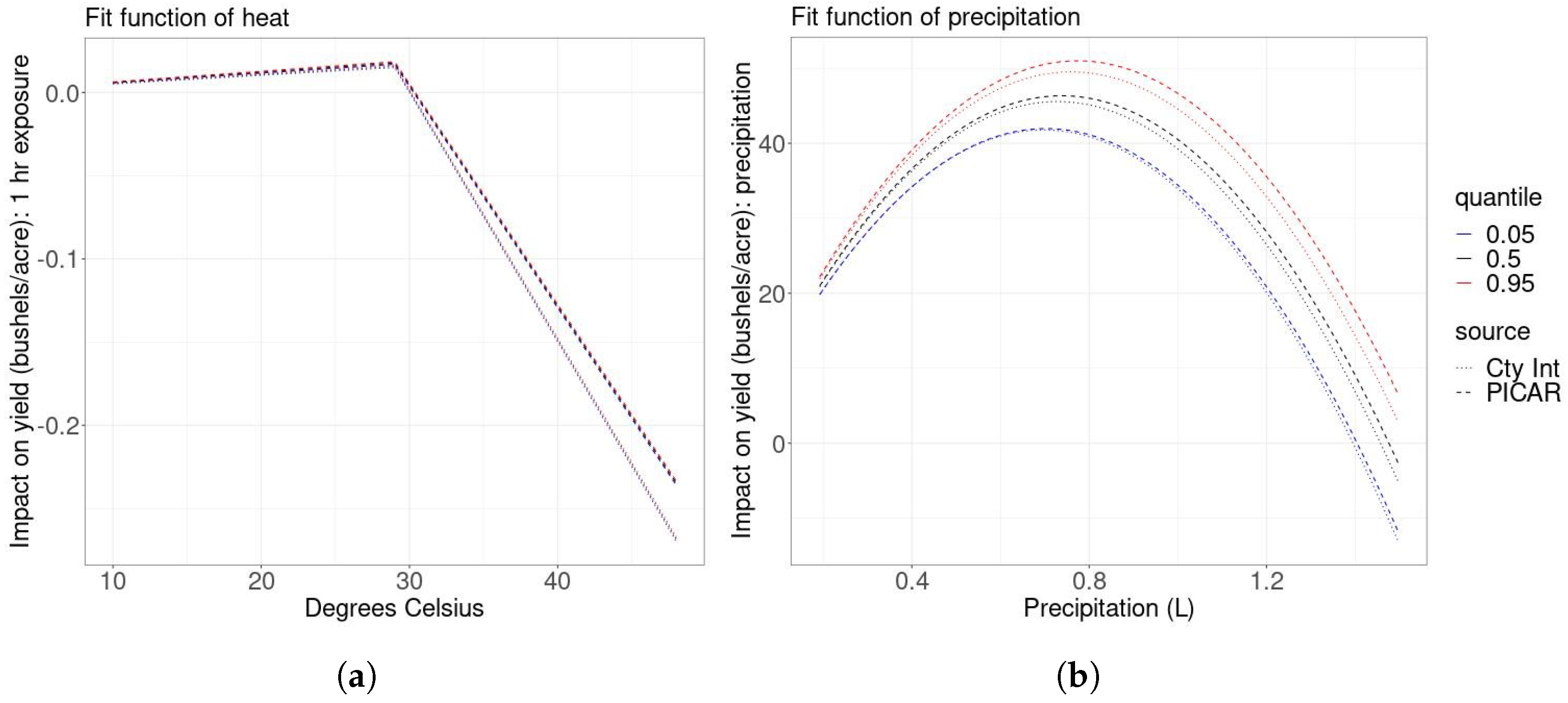
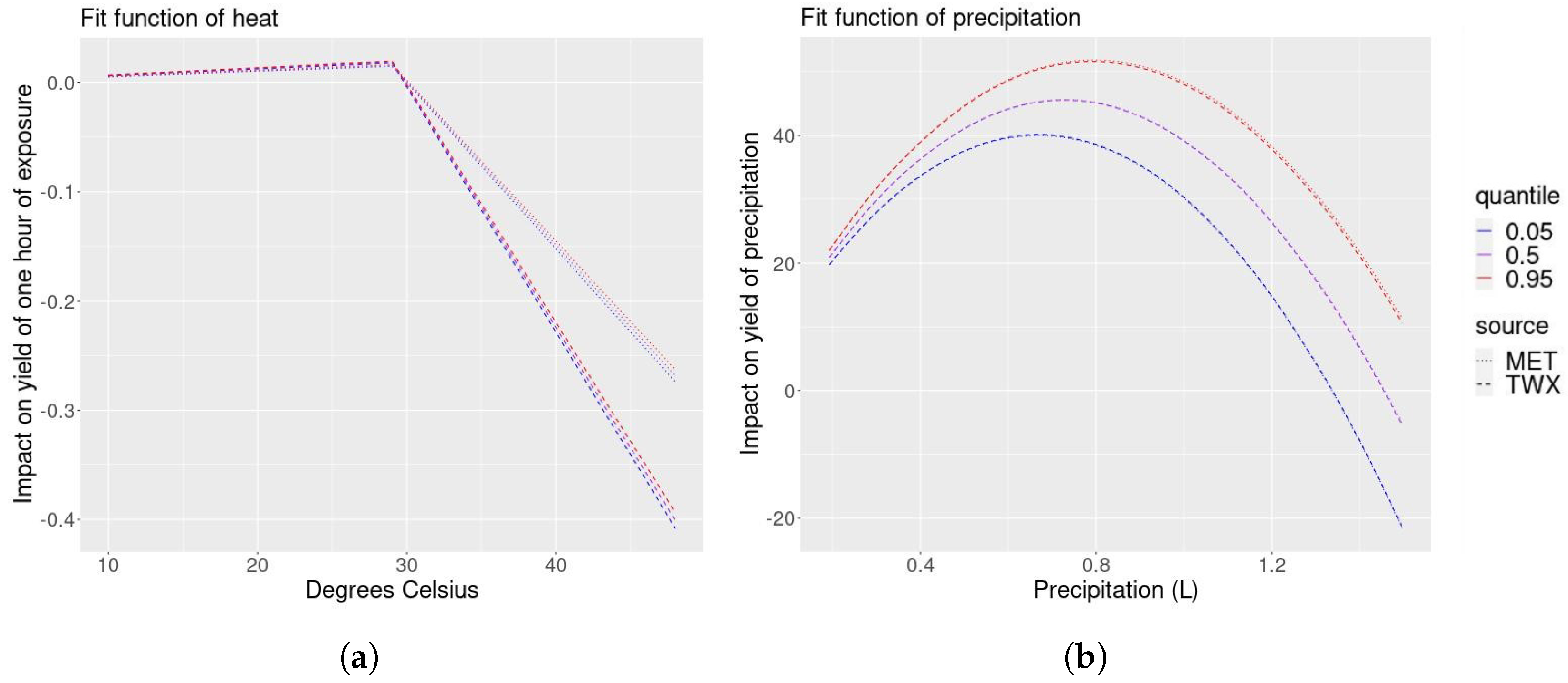
We first consider the modeled relationships between the weather variables of interest, the precipitation and temperature, and the corn yield. In Figure 1a, we display the impact of an additional hour of exposure to each 1 °C temperature interval during the growing season on yields (bushels/acre). We find that exposure to temperatures between 10 °C and 29 °C has a weakly increasingly positive impact on yields, while exposure to temperatures above 29 °C has a strongly increasingly negative impact on yields, the same type of relationship found by [5]. Figure 1b summarizes the quadratic relationship between the total growing season precipitation and yields. We find that increasing the total precipitation up to around 0.8 L during the growing season has a decreasingly positive impact on yields. Above 0.8 L, increasing total growing season precipitation has an increasingly negative impact on yield.
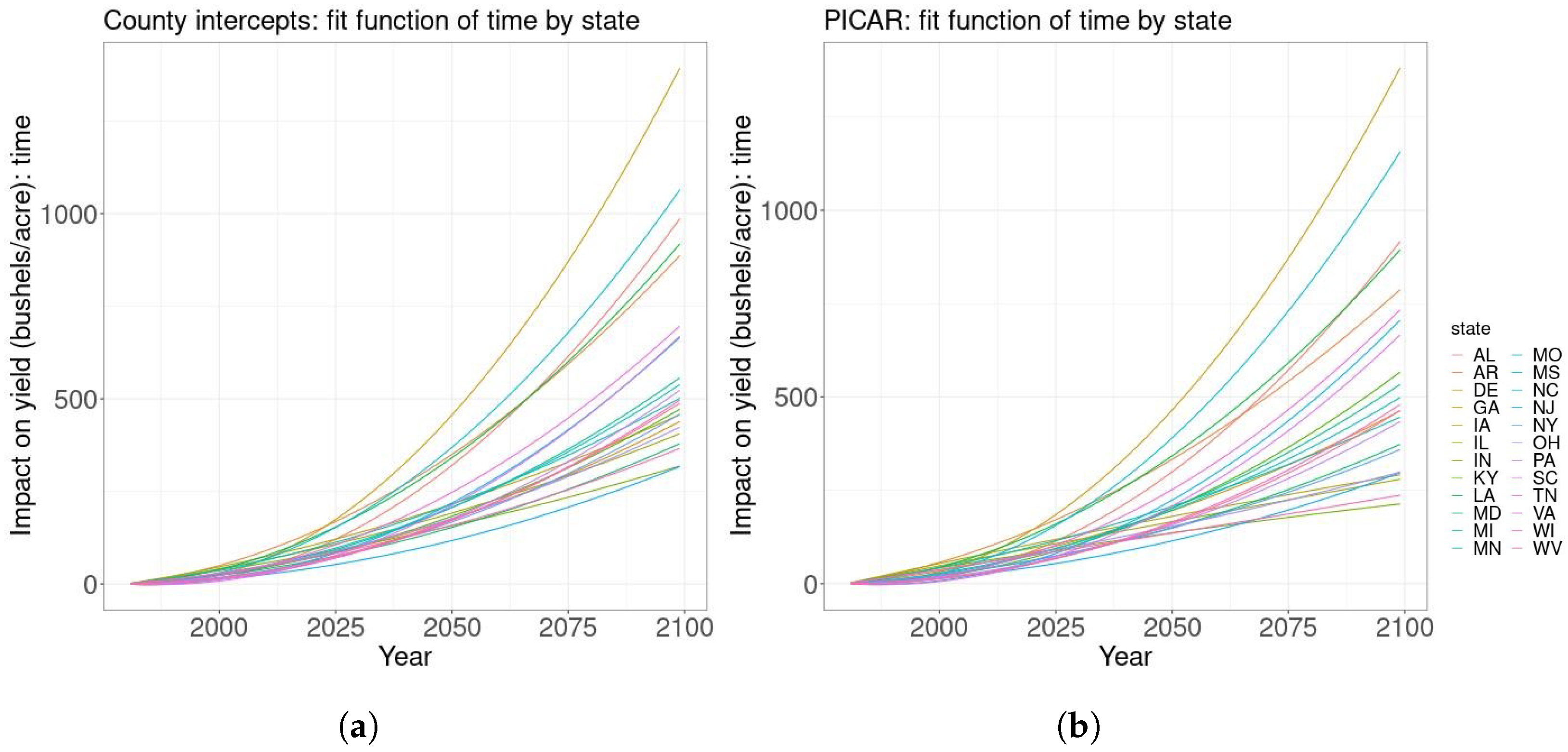
We also consider the impacts of the mean fit quadratic time trend by state from the historical period to what they would be the end of the 21st century. Both the PICAR and county intercepts models give that the impact of time on yields is generally positive to varying degrees for all states (Figure 2a,b). In some states such as Georgia, the estimated impact of temporal factors at the end of the century would be enormous. However, extrapolating the impact of time to the end of the century may not produce realistic results, so we project the detrended yield instead.
For the sake of brevity, we only evaluate how the county intercepts model changes when the TopoWX temperatures replace METDATA temperatures. The relationship between the precipitation and yields is virtually unchanged when we replace METDATA temperatures with TopoWX temperatures, which is desirable since the precipitation dataset has not changed (Figure 3b). When we replace METDATA temperatures with TopoWX temperatures, (1) exposure to temperatures between 10 °C and 29 °C has a slightly more increasingly positive impact on yields and (2) exposure to temperatures above 29 °C has an even more strongly increasingly negative impact on yields (Figure 3a). In summary, switching METDATA for TopoWX temperatures increases the slopes in the piecewise linear relationship between the temperature and yields.
3.2. Predictive Performance
We compare the performances of the county intercepts model to the PICAR model based on the prediction of withheld data. We choose the Widely Applicable Information Criterion (WAIC), a measure of predictive accuracy that averages over the posterior distribution rather than conditioning on a point estimate [42]. We select the final four years (2015–2018) as our validation set since we are interested in making future projections with our models. For both models, the median distance of the prediction to the observation is less than 10% of the observation. Hence, we judge that their predictive abilities are adequate.
Overall, the county intercepts model has a slightly improved predictive ability compared to the PICAR model, but this difference is small considering the scale of the data values. The yield observations have 1st, 25th, 50th, 75th, and 99th quantiles of 33, 86, 111, 139, and 201 bushels/acre. We hypothesize that this is because this model’s indirect representation of spatial correlation is much higher dimensional. The county intercepts model has RMSE of 21.2 bushels/acre; the PICAR model has RMSE of 24.9 bushels/acre (Table 1). The county intercepts model has a WAIC of 858,544, and the PICAR model has a WAIC of 901,826.6 (Table 1). Lower WAIC values indicate a better predictive ability. The county intercepts model’s WAIC is less than 5% smaller than the PICAR model’s WAIC.
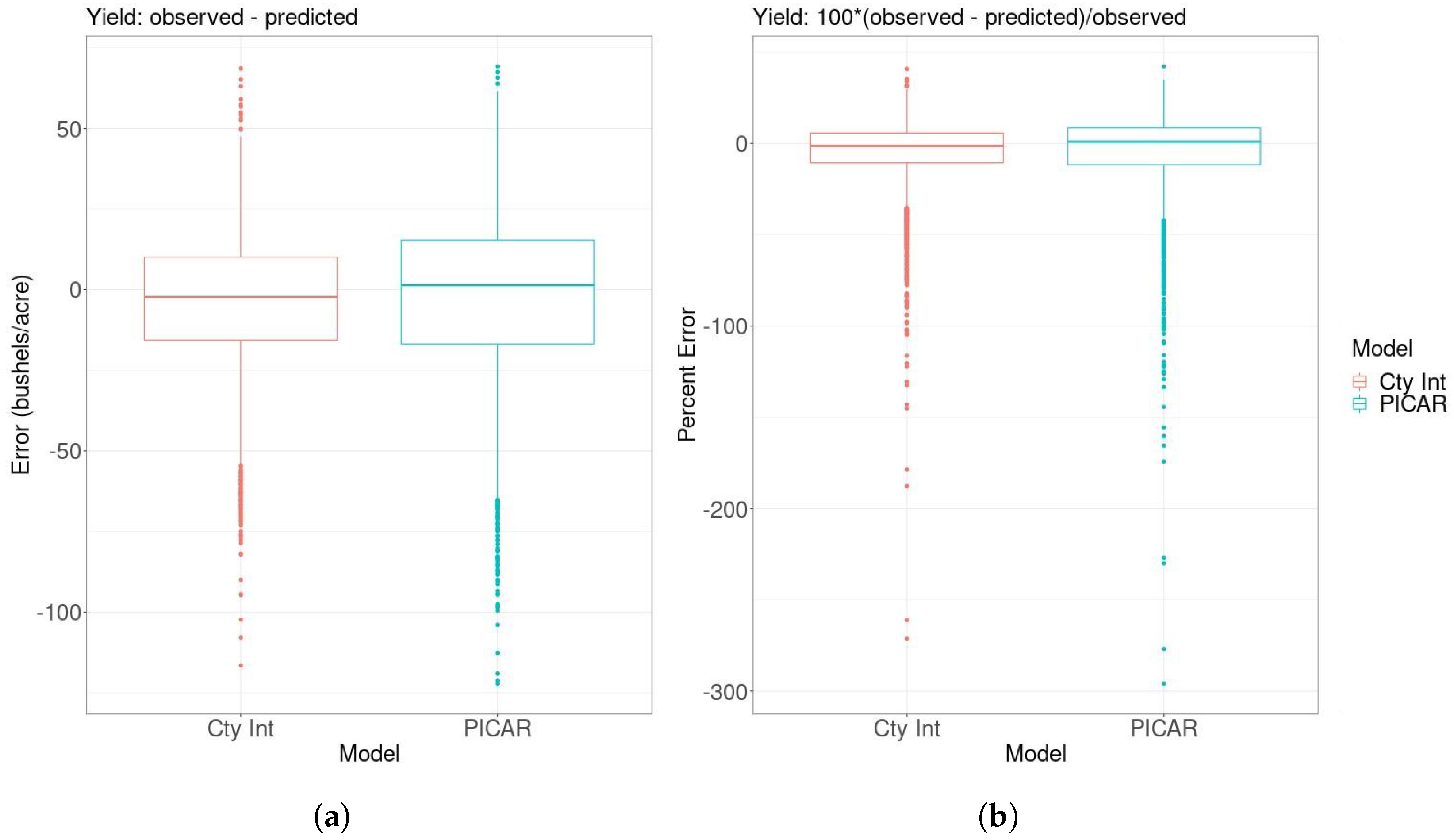
For each year, the county intercepts model is slightly more accurate but again small relative to the data scale (Table 2). Although the last held-out year has the highest RMSE for both models, the trend is that the RMSE values decrease from 2015–2017. We hence see no evidence for a potentially concerning increasing trend in RMSE. The distribution of prediction errors is approximately symmetric around zero for each approach (Figure 4a,b). However, there are generally more cases of predictions that are much too high than much too low.
The county intercepts model and PICAR model produce similar projections. The PICAR model, however, takes considerably less time to approximate the posterior distribution. The PICAR model has a mean effective sample size (ESS) per second of 151 and a minimum ESS/second of 48.2. Meanwhile, the county intercepts model has a mean ESS/second of 2.98 and a min ESS/second of 2.66. We take enough approximate posterior samples so that the ESS for each parameter is at least 10,000. The BIC criterion selects a relatively low rank of Moran’s basis function matrix and mesh density, contributing to the computational efficiency.
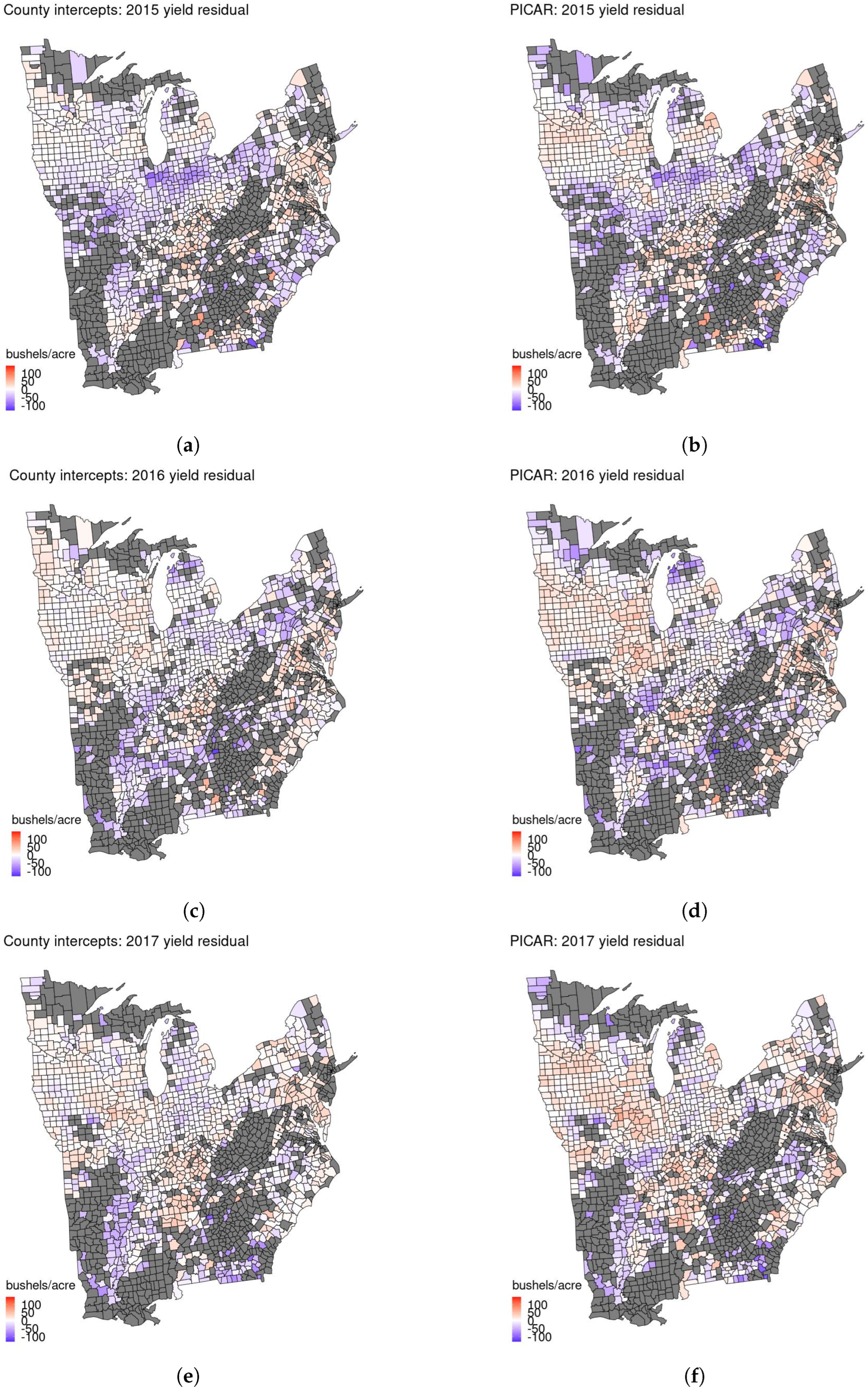
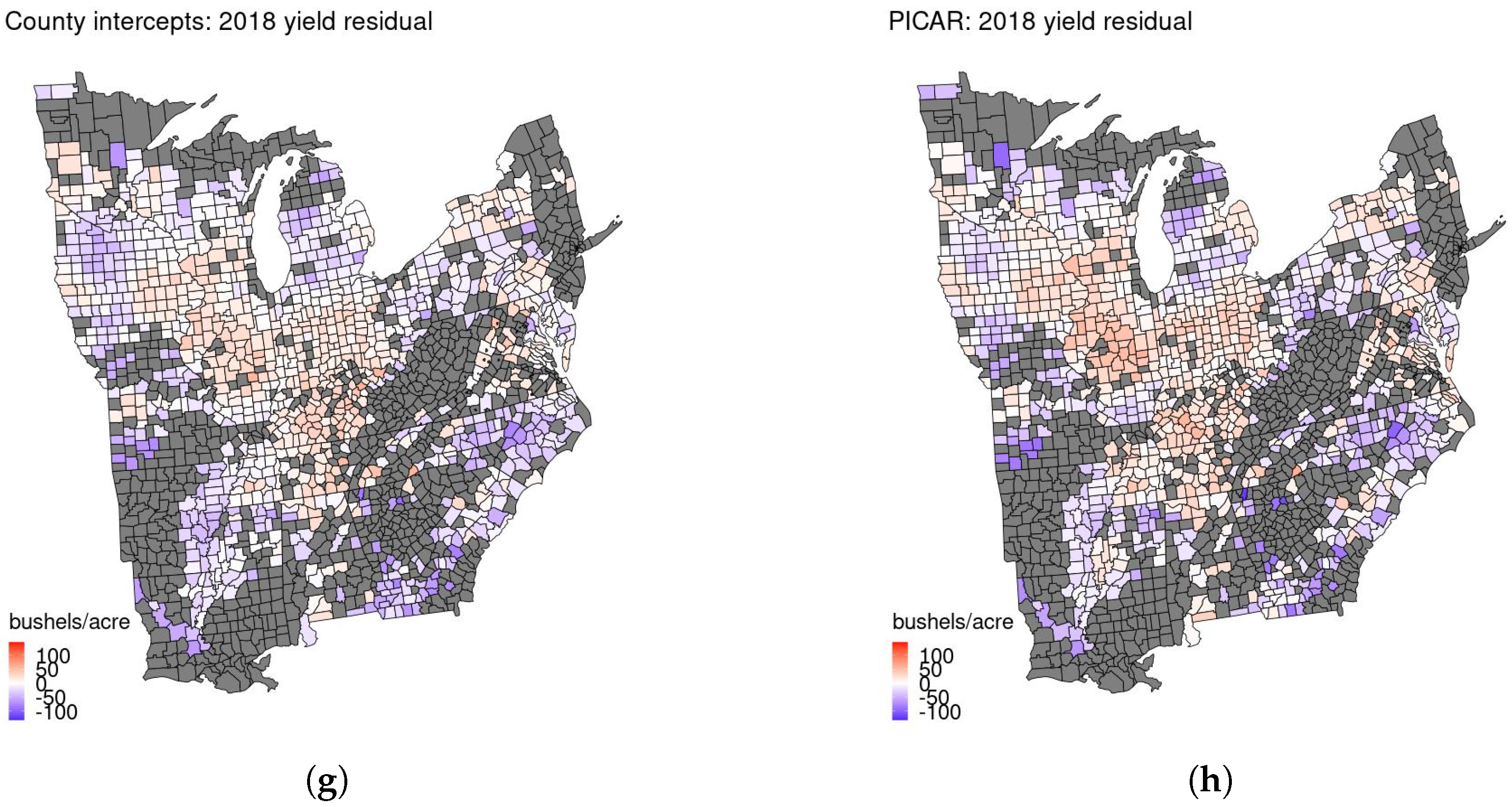
Generally, the remaining spatial patterns in the residuals (observed–predicted crop yield) are similar across all models for all held-out years (Figure 5a–h). For 2018 (Figure 5g,h), the county intercepts approach overpredicts the yield a bit more in parts of Iowa. The PICAR model overpredicts the yield a bit more in a few other counties and years. Again, these differences are not large relative to the scale of the corn yields. The largest overestimates of yields from both models tend to occur in Georgia. We hypothesize that this is due to the fit of the quadratic time trend by state.
We compare the predictive performances of the county intercepts model fit with METDATA to the county intercepts model fit with TopoWX data on two years of held-out data (2015–2016). Note that we are comparing these models using only two years of held-out data now since TopoWX is only available up to 2016.
For 2015–2016, the model fit using temperatures from the TopoWX dataset has a very slightly improved predictive ability compared to the model fit with temperatures from the METDATA dataset (Table 3). Even so, this difference is small considering the scale of the data values. The model fit with TopoWX data has RMSE of 21.2 bushels/acre; the model fit with METDATA has RMSE of 21.3 bushels/acre. The model fit with METDATA has a WAIC of 858,544, and the model fit with TopoWX data has a WAIC of 853,522. The model fit with TopoWX temperatures has a WAIC less than 1% smaller than that of the model fit with METDATA temperatures. We also consider RMSE for each held-out year of data individually using the model fit with each temperature dataset (Table 4). For 2015, the model fit with TopoWX temperatures is slightly more accurate. For 2016, the model fit with METDATA temperatures is slightly more accurate.
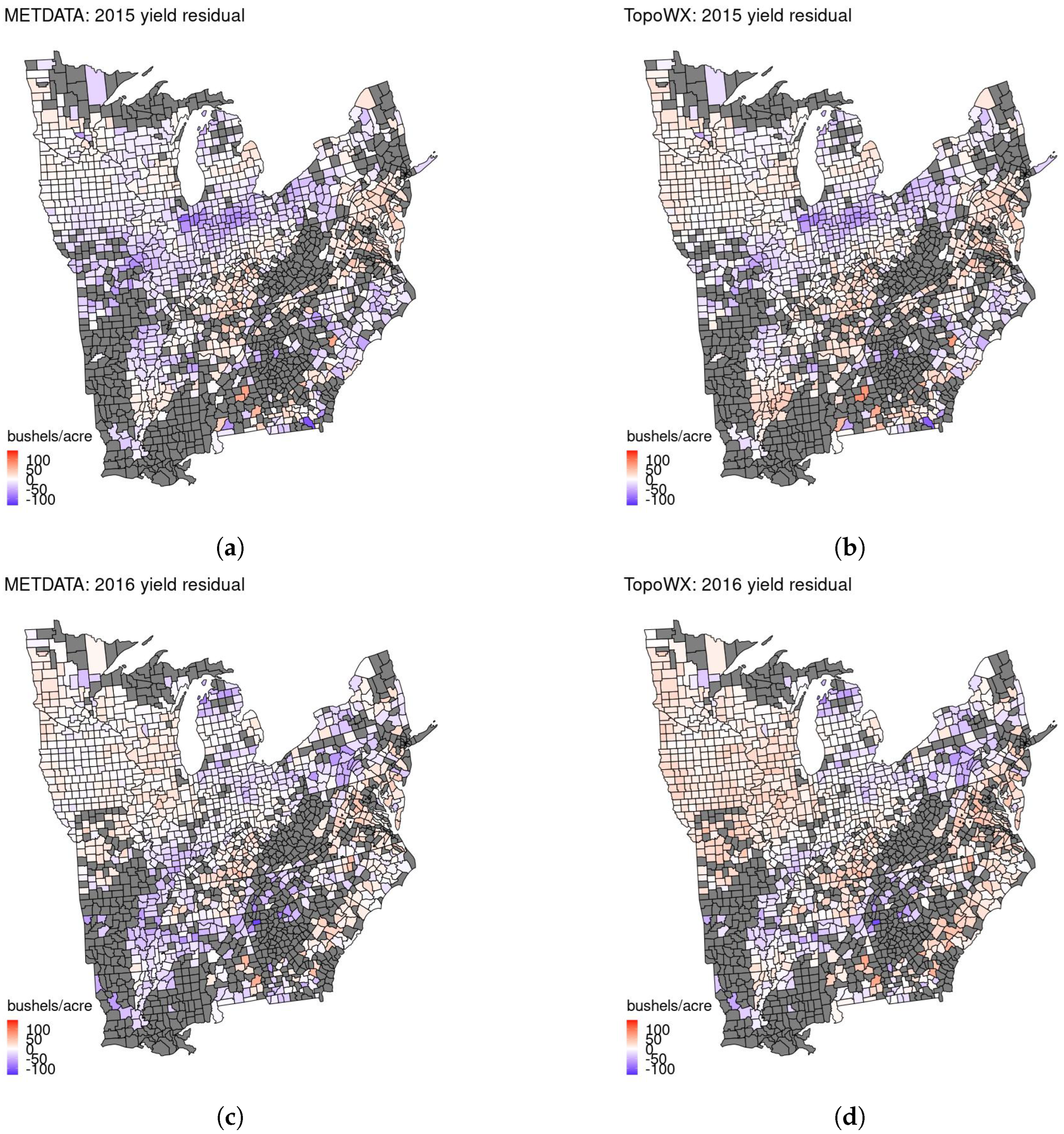
We also consider how the residuals in space compare when the TopoWX temperatures are used in place of the METDATA temperatures (Figure 6). The spatial patterns in the residuals are generally similar for both for held-out years. For 2015, the spatial plots of yield residuals are nearly indistinguishable. For 2016, the model fit with TopoWX temperatures appears to overpredict slightly more than the model fit with METDATA in Iowa.
3.3. Projections
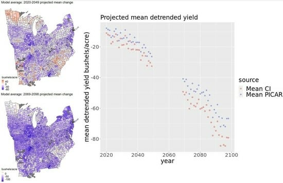
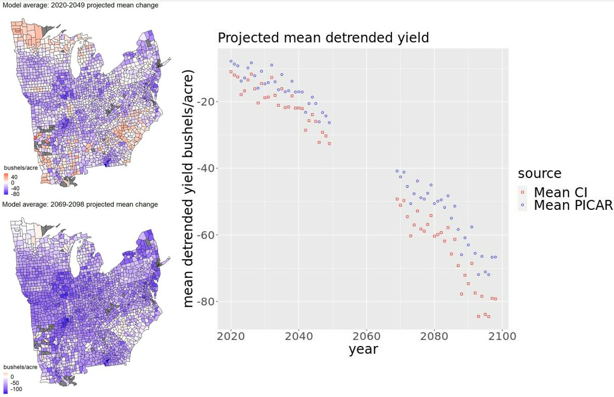
We consider two projection periods, the near future (2020–2049) and the end of the 21st century (2069–2098). For each projection period and statistical model, we display the change in mean yield averaged over all years for each county (Figure 7). To compute these values, we first obtain a sample of detrended yield projections at each county and year. The sample contains a detrended yield projection corresponding to each climate model and each posterior parameter sample. We weight the samples equally to compute the mean projection for each county and year. We average these projections over all years in the projection period to obtain a mean detrended yield value for each county. To obtain the historical mean detrended county yield, we average the historical estimated detrended yields over all years for each county. For each county, we subtract the historical mean detrended county yield from the projected mean detrended county yield to obtain the projected change in yield.
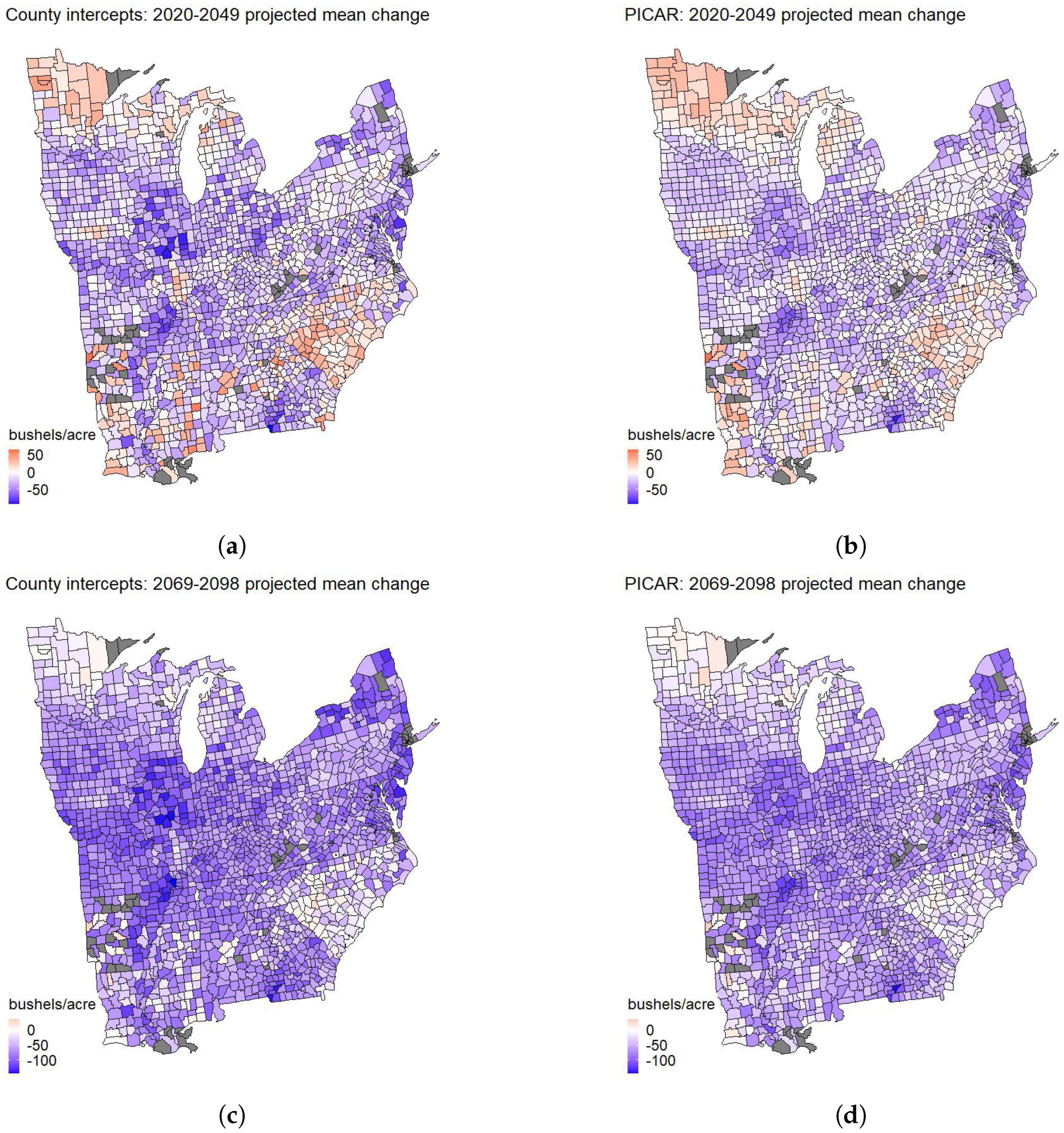
For both projection periods, both statistical models mostly project decreases in mean yield over the region of interest and greater decreases in 2069–2098. For 2020–2049, the county intercepts model projects a decrease in mean yield in 79.0% of counties and the PICAR model projects a decrease in mean yield in 77.4% of counties. By 2069–2098, the county intercepts model projects a decrease in mean yield in 96.3% of counties and the PICAR model projects a decrease in mean yield in 96.3% of counties. For all models and in both projection periods, a small number of counties (67 out of 1821) in both the south and the north experience increases in both projection periods and across all statistical models. In both 2020–2049 and 2069–2098, the spatial patterns in the projections are generally similar between the PICAR model and the county intercepts model. However, in some counties the changes projected by the county intercepts model are more extreme.
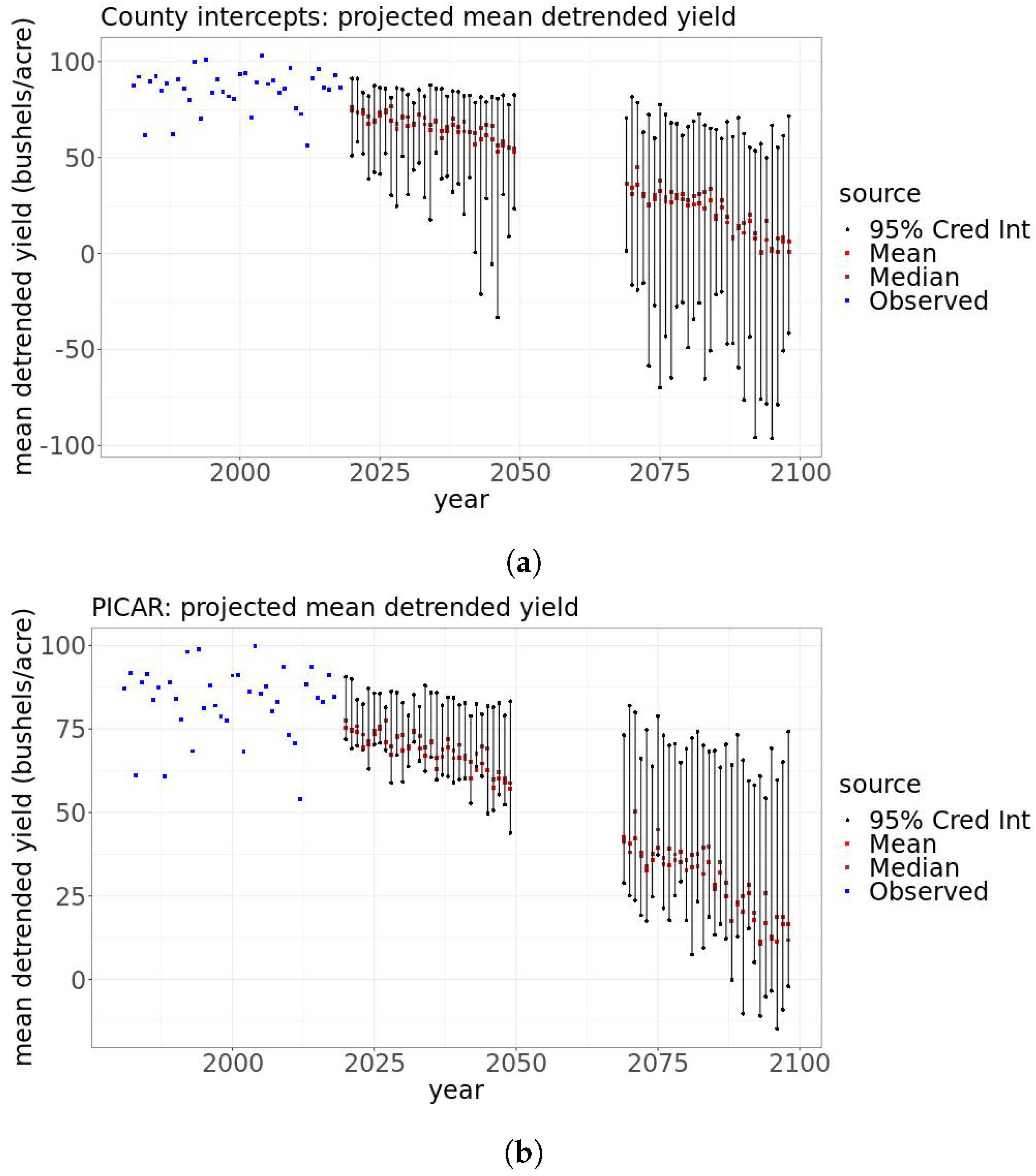
For each statistical model, we also project and characterize uncertainty surrounding the mean detrended yield for each year averaged over all counties (Figure 8). Broadly, the uncertainties we characterize are from the statistical model parameter posteriors and the differing projections of 18 bias-corrected climate models. To average the yearly mean yield over all counties, we weight each county by its last reported growing area. We compute the bounds of the 95% credible interval to summarize the uncertainty surrounding these projections. To obtain these bounds, we first obtain a projection of yearly mean detrended yield using each climate model at each step of the 1000 steps of the thinned parameter posterior sample. We then have a sample of 18,000 projections of the mean detrended yield for each year. Considering all climate models and all posterior parameter samples to be equally likely, we set the 2.5 and 97.5% quantiles of each year’s sample of projections to be the bounds of the 95% credible interval. For each year, we take the mean of this sample as the mean projection.
As the century progresses, increasing uncertainty surrounds decreasing detrended mean projections from both statistical models. The county intercepts model (Figure 8a) gives a smaller mean projection and wider credible intervals than the PICAR model does (Figure 8b). Averaged over 2020–2049 (2069–2098), the county intercepts model projects the detrended mean yearly yield to be 23.7% (76.4%) smaller than the historical detrended mean yearly yield. For 2020–2049 (2069–2098), the 95% credible interval bounds range from 6.63% larger to 139% smaller (4.44% to 213% smaller) than the historical detrended mean. Averaged over 2020–2049 (2069–2098), the PICAR model projects the detrended mean yearly yield to be 18.9% (65.8%) smaller than the historical detrended mean yearly yield. The 95% credible interval bounds range from 8.75% larger to 47.4% smaller (1.68% to 118% smaller) than the historical detrended mean.
Our two statistical models provide similar results in terms of yearly means and spatial patterns of projected changes in corn yields. The uncertainties surrounding the detrended mean yield projections are large and become larger later in the century. Overall, our results from both statistical models considering parametric and climate model choice uncertainty project that climate change will negatively impact mean corn yields by the end of the century. Compared to [5], we find greater decreases in yields by the end of the century. Compared to the results of [9], which considers parametric uncertainty through pre-calibration, we generally find less uncertainty in our projections.
4. Discussion
We compare two statistical models that differ in their treatment of county-level spatial effects. One novelty of our work is the use of spatial basis representations, specifically following the PICAR approach, in projecting corn yields. The county intercepts model employing a random intercept for each county is commonly used. We find that the predictive performances of both approaches are similarly satisfactory relative to the scale of the data. However, the PICAR approach is approximately four times faster; we hypothesize that this speed-up will be more dramatic with a greater number of observations. For both models, the relationship between heat and corn yields is broadly similar to that reported by [5]. Similarly to previous studies, both models project an increasingly negative impact of climate change on corn yields as the century progresses [5,9]. Using our Monte Carlo-based approach and an ensemble of 18 climate models, we account for both parametric uncertainty and model uncertainty in these projections.
We also compare statistical models fit with different gridded temperature data products. One only uses weather station data and one combines weather station and remotely sensed data. The modeled relationships are broadly similar, but temperature has a stronger effect on yields according to the model fit with the weather station and remotely sensed data product. Using this data product also yields a model with a slightly improved predictive ability in our data-rich area of interest. If we were to use a data product that combines weather station and remotely sensed temperatures in a region where weather stations are sparser, the increase in model performance and differences in modeled relationships would likely be more pronounced.
Our statistical modeling framework is subject to several caveats. We assume that the estimated statistical relationship between historical weather and yields will hold in the future. The relationship between weather and yields may change given crop adaptation or new technology [47]. Although indirectly accounted for by removing the time trend, we do not explicitly include measurements of carbon dioxide [48] or air pollution [49], which may impact yields. For this reason, our projected changes in yields should be interpreted as changes only due to the climate. Our treatment of parametric uncertainty assumes the structure of our statistical model relating corn yields to weather is correct, but other model structures could be chosen. For example, recent work suggests that compound hydroclimatic extremes may be more valuable than individual extremes and soil moisture may be more useful than precipitation for predicting corn yield variations [50]. Our model considers individual extremes and precipitation. We also do not consider that the spatial distribution of crops may change, which could mitigate the negative impacts of climate change on yields [11].
In addition, we do not account for errors in historical weather observations or in our estimate of the amount of time crops are exposed to each 1 °C interval. Errors in weather variable measurements and estimates could obscure the relationship between corn yields and our weather variables. Our PICAR-based spatial random effects or random county intercepts are impacted by how well the chosen functions of weather variables account for variability in corn yields. In our model, we treat the bias-corrected climate model output as equivalent to weather observations, but there are major differences between them [10]. We consider the business-as-usual forcing scenario in our projections. Some argue that a scenario with no mitigation measures or no additional mitigation measures beyond what currently exists is highly unlikely [51]. Still, our recent emissions mirror the emissions trajectory associated with RCP 8.5 [52]. Although International Energy Agency (IEA) emissions projections lie between RCP 4.5 and RCP 8.5 [53,54], missing climate cycle carbon feedbacks impact IEA emissions scenarios by increasing them towards cumulative emissions consistent with RCP 8.5 [52]. The plausibility of the world following an emissions trajectory like that of RCP 8.5 is the subject of active scholarly debate.
We also assume that county-level spatial effects will remain constant in the future. While we deal with time-constant spatial correlation in the residuals using the PICAR approach, there is still lingering spatial correlation in the residuals. We hypothesize that this is mainly because the spatial effects are constant in time. Time-varying spatial effects may more completely account for the spatial patterns in the residuals. We could then subtract these effects and project the weather-only part of corn yields [10]. However, a model with spatiotemporal random effects would take much longer to fit due to the increased number of parameters.
5. Conclusions
In summary, we consider two types of statistical models: one that indirectly deals with spatial correlation via a random effect for each county (county intercepts) and one that directly deals with spatial correlation via spatial basis functions (PICAR). We compare them in terms of (1) relationships between weather variables and corn yields, (2) predictive performance, and (3) projections considering key uncertainties. We find broadly similar impacts of weather variables and predictive abilities between these two types of models. The PICAR model projects slightly less drastic decreases in corn yield with less uncertainty than the county intercepts model. The PICAR model also boasts computational savings, but the county intercepts model has a slightly better predictive accuracy. When we replace temperatures from a gridded weather station data product (METDATA) with temperatures from a gridded data product that combines weather station and satellite data (TopoWX), we also see models with broadly similar weather variable impacts and predictive abilities. However, using temperatures from TopoWX slightly magnifies the impact of temperature on corn yields. Overall, the choice of the representation of spatial effects and the choice of temperature data product impact modeled relationships and predictive accuracy, but results are still broadly similar. This research demonstrates the importance of accounting for uncertainty surrounding model choice and weather data sources on model inference and or projections.
Supplementary Materials
The following supporting information can be downloaded at: https://www.mdpi.com/article/10.3390/rs16010069/s1, Figure S1: Fit relationship between heat exposure and yield with based on the middle 90% of MCMC samples of the coefficient posteriors; Figure S2: Fit relationships between time and yield for each state based on the means of the coefficient posteriors; Figure S3: Distribution of prediction errors from the CI, PICAR(BIC) and PICAR (AIC) models. Figure S4: Residuals in space for each held out year (2015–2018) with the CI model (top row), PICAR (BIC) model (middle row), and PICAR (BIC) model (bottom row); Table S1: Predictive performance on held out years.
Author Contributions
Conceptualization, M.H., K.K., B.S.L. and R.E.N.; methodology, S.R., B.S.L. and M.H.; formal analysis, S.R.; resources, M.H., K.K. and R.E.N.; data curation, S.R.; writing—original draft preparation, S.R.; writing—review and editing, S.R., B.S.L., R.E.N., K.K., and M.H.; visualization, S.R.; supervision, M.H., K.K., B.S.L. and R.E.N.; project administration, R.E.N., K.K. and M.H.; funding acquisition, R.E.N., K.K. and M.H. All authors have read and agreed to the published version of this manuscript.
Funding
This work was supported by the U.S. Department of Energy, Office of Science, Biological and Environmental Research Program, Earth and Environmental Systems Modeling, MultiSector Dynamics under cooperative agreements DE-SC0016162 and DE-SC0022141. Additional support was provided by the Penn State Center for Climate Risk Management and the Thayer School of Engineering at Dartmouth College. Any opinions, findings, and conclusions or recommendations expressed in this material are those of the authors and do not necessarily reflect the views of the US Department of Energy or other funding entities.
Data Availability Statement
The data and code presented in this study are openly available at the MSDLive Data Repository under the same title as the manuscript.
Acknowledgments
We are very grateful to Haochen Ye for the R codes, which he kindly made available on his GitHub page: https://github.com/yhaochen/Climate_CornYield. We accessed this webpage last on 15 September 2022. Computations for this research were performed on the Pennsylvania State University’s Institute for Computational and Data Sciences’ Roar supercomputer. We thank Skip Wishbone and Siggi Snyder for their invaluable inputs.
Conflicts of Interest
The authors declare no conflicts of interest.
References
- USDA. Feedgrains Sector at a Glance. 2022. Available online: https://www.ers.usda.gov/topics/crops/corn-and-other-feedgrains/feedgrains-sector-at-a-glance/ (accessed on 7 September 2021).
- Lobell, D.B.; Burke, M.B. On the use of statistical models to predict crop yield responses to climate change. Agric. For. Meteorol. 2010, 150, 1443–1452. [Google Scholar] [CrossRef]
- Roberts, M.J.; Braun, N.O.; Sinclair, T.R.; Lobell, D.B.; Schlenker, W. Comparing and combining process-based crop models and statistical models with some implications for climate change. Environ. Res. Lett. 2017, 12, 095010. [Google Scholar] [CrossRef]
- Mendelsohn, R.; Nordhaus, W.D.; Shaw, D. The Impact of Global Warming on Agriculture: A Ricardian Analysis. Am. Econ. Rev. 1994, 84, 753–771. [Google Scholar]
- Schlenker, W.; Roberts, M.J. Nonlinear temperature effects indicate severe damages to U.S. crop yields under climate change. Proc. Natl. Acad. Sci. USA 2009, 106, 15594–15598. [Google Scholar] [CrossRef]
- Wuebbles, D.; Easterling, D.; Hayhoe, K.; Knutson, T.; Kopp, R.; Kossin, J.; Kunkel, K.; LeGrande, A.; Mears, C.; Sweet, W.; et al. Our globally changing climate. In Climate Science Special Report: Fourth National Climate Assessment, Volume I; 2016; pp. 35–72. [Google Scholar] [CrossRef]
- Wing, I.S.; Monier, E.; Stern, A.; Mundra, A. US major crops’ uncertain climate change risks and greenhouse gas mitigation benefits. Environ. Res. Lett. 2015, 10, 115002. [Google Scholar] [CrossRef]
- Li, X.; Takahashi, T.; Suzuki, N.; Kaiser, H.M. The impact of climate change on maize yields in the United States and China. Agric. Syst. 2011, 104, 348–353. [Google Scholar] [CrossRef]
- Ye, H.; Nicholas, R.E.; Roth, S.; Keller, K. Considering uncertainties expands the lower tail of maize yield projections. PLoS ONE 2021, 16, e0259180. [Google Scholar] [CrossRef]
- Lafferty, D.C.; Sriver, R.L.; Haqiqi, I.; Hertel, T.W.; Keller, K.; Nicholas, R.E. Statistically bias-corrected and downscaled climate models underestimate the adverse effects of extreme heat on U.S. maize yields. Nat. Commun. Earth Environ. 2021, 2, 196. [Google Scholar] [CrossRef]
- Leng, G.; Huang, M. Crop yield response to climate change varies with crop spatial distribution pattern. Sci. Rep. 2017, 7, 1463. [Google Scholar] [CrossRef]
- Lesk, C.; Coffel, E.; Horton, R. Net benefits to US soy and maize yields from intensifying hourly rainfall. Nat. Clim. Chang. 2020, 10, 819–822. [Google Scholar] [CrossRef]
- Conley, T. GMM estimation with cross sectional dependence. J. Econom. 1999, 92, 1–45. [Google Scholar] [CrossRef]
- Lee, B.S.; Haran, M. PICAR: An Efficient Extendable Approach for Fitting Hierarchical Spatial Models. Technometrics 2022, 64, 187–198. [Google Scholar] [CrossRef]
- Cairns, J.E.; Chamberlin, J.; Rutsaert, P.; Voss, R.C.; Ndhlela, T.; Magorokosho, C. Challenges for sustainable maize production of smallholder farmers in sub-Saharan Africa. J. Cereal Sci. 2021, 101, 103274. [Google Scholar] [CrossRef]
- Trewin, B.; Adam, J.P.; Almadjir, M.R.; Alvar-Beltrán, J.; Ba, M.N.; Babiker, A.S.; Baddour, O.; Blunden, J.; Bennani, H.A.; Cazanave, A.; et al. State of the Climate in Africa 2019; Technical Report; World Meteorological Organization: Geneva, Switzerland, 2020. [Google Scholar]
- Uddstrom, M.J. Retrieval of Atmospheric Profiles from Satellite Radiance Data by Typical Shape Function Maximum a Posteriori Simultaneous Retrieval Estimators. J. Appl. Meteorol. Climatol. 1988, 27, 515–549. [Google Scholar] [CrossRef]
- Tomlinson, C.J.; Chapman, L.; Thornes, J.E.; Baker, C. Remote sensing land surface temperature for meteorology and climatology: A review. Met. Apps. 2011, 18, 296–306. [Google Scholar] [CrossRef]
- Konik, M.; Kowalewski, M.; Bradtke, K.; Darecki, M. The operational method of filling information gaps in satellite imagery using numerical models. Int. J. Appl. Earth Obs. Geoinf. 2019, 75, 68–82. [Google Scholar] [CrossRef]
- Ruzmaikin, A.; Aumann, H.H.; Lee, J.; Susskind, J. Diurnal Cycle Variability of Surface Temperature Inferred From AIRS Data. J. Geophys. Res. Atmos. 2017, 122, 10,928–10,938. [Google Scholar] [CrossRef]
- NASS. Crop Production Historical Track Records 2018. Available online: http://quickstats.nass.usda.gov (accessed on 5 October 2021).
- Abatzoglou, J. Development of gridded surface meteorological data for ecological applications and modelling. Int. J. Climatol. 2013, 33, 121–131. [Google Scholar] [CrossRef]
- Hoffman, A.; Kemanian, A.; Forest, C. The response of maize, sorghum, and soybean yield to growing-phase climate revealed with machine learning. Environ. Res. Lett. 2020, 15, 094013. [Google Scholar] [CrossRef]
- Abatzoglou, J.; Brown, T. A comparison of statistical downscaling methods suited for wildfire applications. Int. J. Climatol. 2012, 32, 772–780. [Google Scholar] [CrossRef]
- Keane, M.; Neal, T. Climate Change and U.S. Agriculture: Accounting for Multi-dimensional Slope Heterogeneity in Production Functions (2 January 2020). UNSW Business School Research Paper No. 2018-08a. Available online: https://ssrn.com/abstract=3180480 (accessed on 17 July 2022). [CrossRef]
- Oyler, J.W.; Dobrowski, S.Z.; Holden, Z.A.; Running, S.W. Remotely Sensed Land Skin Temperature as a Spatial Predictor of Air Temperature across the Conterminous United States. J. Appl. Meteorol. Climatol. 2016, 55, 1441–1457. [Google Scholar] [CrossRef]
- Wan, Z.; Hook, S.; Hulley, G. MODIS/Aqua Land Surface Temperature/Emissivity 8-Day L3 Global 1km SIN Grid V061. Available online: https://lpdaac.usgs.gov/products/mod11a2v061/ (accessed on 17 July 2022).
- Muñoz Sabater, J. ERA5-Land Hourly Data from 1950 to Present. Available online: https://cds.climate.copernicus.eu/cdsapp#!/dataset/10.24381/cds.e2161bac?tab=overview (accessed on 17 July 2022).
- Saha, S.; Moorthi, S.; Pan, H.L.; Wu, X.; Wang, J.; Nadiga, S.; Tripp, P.; Kistler, R.; Woollen, J.; Behringer, D.; et al. The NCEP Climate Forecast System Reanalysis. Bull. Am. Meteorol. Soc. 2010, 91, 1015–1058. [Google Scholar] [CrossRef]
- Haining, R. Spatial Data Analysis in the Social and Environmental Sciences; Cambridge University Press: Cambridge, UK, 1990. [Google Scholar] [CrossRef]
- Legendre, P. Spatial Autocorrelation: Trouble or New Paradigm? Ecology 1993, 74, 1659–1673. [Google Scholar] [CrossRef]
- Gumpertz, M.L.; Graham, J.M.; Ristaino, J.B. Autologistic Model of Spatial Pattern of Phytophthora Epidemic in Bell Pepper: Effects of Soil Variables on Disease Presence. J. Agric. Biol. Environ. Stat. 1997, 2, 131–156. [Google Scholar] [CrossRef]
- Christensen, O.F.; Roberts, G.O.; Sköld, M. Robust Markov chain Monte Carlo methods for spatial generalized linear mixed models. J. Comput. Graph. Stat. 2006, 15, 1–17. [Google Scholar] [CrossRef]
- Haran, M.; Hodges, J.S.; Carlin, B.P. Accelerating computation in Markov random field models for spatial data via structured MCMC. J. Comput. Graph. Stat. 2003, 12, 249–264. [Google Scholar] [CrossRef]
- Cressie, N.; Sainsbury-Dale, M.; Zammit-Mangion, A. Basis-Function Models in Spatial Statistics. Annu. Rev. Stat. Its Appl. 2022, 9, 373–400. [Google Scholar] [CrossRef]
- Cressie, N.; Johannesson, G. Fixed rank kriging for very large spatial data sets. J. R. Stat. Soc. Ser. B (Stat. Methodol.) 2008, 70, 209–226. [Google Scholar] [CrossRef]
- Hughes, J.; Haran, M. Dimension reduction and alleviation of confounding for spatial generalized linear mixed models. J. R. Stat. Soc. Ser. B (Stat. Methodol.) 2013, 75, 139–159. [Google Scholar] [CrossRef]
- Hjelle, Ø.; Dæhlen, M. Triangulations and Applications; Springer Science & Business Media: Berlin/Heidelberg, Germany, 2006. [Google Scholar]
- Lindgren, F.; Rue, H. Bayesian Spatial Modelling with R-INLA. J. Stat. Softw. Artic. 2015, 63, 1–25. [Google Scholar] [CrossRef]
- Akaike, H. A new look at the statistical model identification. IEEE Trans. Autom. Control 1974, 19, 716–723. [Google Scholar] [CrossRef]
- Schwarz, G. Estimating the Dimension of a Model. Ann. Stat. 1978, 6, 461–464. [Google Scholar] [CrossRef]
- Gelman, A.; Hwang, J.; Vehtari, A. Understanding predictive information criteria for Bayesian models. Stat. Comput. 2014, 24, 997–1016. [Google Scholar] [CrossRef]
- R Core Team. R: A Language and Environment for Statistical Computing; R Foundation for Statistical Computing: Vienna, Austria, 2022. [Google Scholar]
- Kass, R.E.; Carlin, B.P.; Gelman, A.; Neal, R.M. Markov Chain Monte Carlo in Practice: A Roundtable Discussion. Am. Stat. 1998, 52, 93–100. [Google Scholar]
- Robert, C.P.; Casella, G. Monte Carlo Statistical Methods; Springer: New York, NY, USA, 2004. [Google Scholar]
- Rice, K. Sprint research runs into a credibility gap. Nature 2004, 432, 147. [Google Scholar] [CrossRef]
- Neal, T.; Keane, M. The Impact of Climate Change on U.S. Agriculture: The Roles of Adaptation Techniques and Emissions Reductions; Discussion Papers 2018-08; School of Economics, The University of New South Wales: Sydney, Australia, 2018. [Google Scholar]
- Moore, F.C.; Baldos, U.L.C.; Hertel, T. Economic impacts of climate change on agriculture: A comparison of process-based and statistical yield models. Environ. Res. Lett. 2017, 12, 065008. [Google Scholar] [CrossRef]
- Lobell, D.B.; Burney, J.A. Cleaner air has contributed one-fifth of US maize and soybean yield gains since 1999. Environ. Res. Lett. 2021, 16, 074049. [Google Scholar] [CrossRef]
- Haqiqi, I.; Grogan, D.S.; Hertel, T.W.; Schlenker, W. Quantifying the impacts of compound extremes on agriculture. Hydrol. Earth Syst. Sci. 2021, 25, 551–564. [Google Scholar] [CrossRef]
- Srikrishnan, V.; Guan, Y.; Tol, R.S.; Keller, K. Probabilistic projections of baseline twenty-first century CO2 emissions using a simple calibrated integrated assessment model. Clim. Chang. 2022, 170, 37. [Google Scholar] [CrossRef]
- Schwalm, C.R.; Glendon, S.; Duffy, P.B. RCP8.5 tracks cumulative CO2 emissions. Proc. Natl. Acad. Sci. USA 2020, 117, 19656–19657. [Google Scholar] [CrossRef]
- Hausfather, Z.; Peters, G.P. Emissions—The ‘business as usual’ story is misleading. Nature 2020, 557, 618–620. [Google Scholar] [CrossRef] [PubMed]
- Skea, J.; van Diemen, R.; Portugal-Pereira, J.; Khourdajie, A.A. Outlooks, explorations and normative scenarios: Approaches to global energy futures compared. Technol. Forecast. Soc. Chang. 2021, 168, 120736. [Google Scholar] [CrossRef]
Figure 1.
Relationships between heat exposure and yield (panel (a)) and total precipitation and yield (panel (b)). Each panel shows the relationship between the climate variable and yield based on the middle 90% of MCMC samples of the parameter posteriors using either the county intercepts or PICAR model. The modeled impact of heat on corn yield is similar to previous studies in both models. The county intercepts model finds more extreme high temperature damages than the PICAR model.

Figure 2.
Mean relationships between time and yield for each state based on the county intercepts model (panel (a)) and the PICAR model (panel (b)). The modeled impact of technology is highly variable by state according to both the county intercepts and PICAR models.
Figure 2.
Mean relationships between time and yield for each state based on the county intercepts model (panel (a)) and the PICAR model (panel (b)). The modeled impact of technology is highly variable by state according to both the county intercepts and PICAR models.

Figure 3.
Relationships between heat exposure and yield (panel (a)) and total precipitation and yield (panel (b)). Each panel shows the relationship between the climate variable and yield based on the middle 90% of MCMC samples of the parameter posteriors where the model is trained using either METDATA or TopoWX temperatures. The modeled impact of heat is more extreme when we replace METDATA with TopoWX temperatures. The precipitation impact is practically unchanged.

Figure 4.
Distribution of prediction errors (panel (a)) in bushels/acre and percent errors (panel (b)) from the county intercepts and PICAR models. The majority of errors are very small relative to scale of the data. Both distributions of errors have long lower tails.
Figure 4.
Distribution of prediction errors (panel (a)) in bushels/acre and percent errors (panel (b)) from the county intercepts and PICAR models. The majority of errors are very small relative to scale of the data. Both distributions of errors have long lower tails.

Figure 5.
Residuals in space for held-out years from county intercepts model (panels (a,c,e,g)) and PICAR model (panels (b,d,f,h)). The patterns are broadly similar for both models.
Figure 5.
Residuals in space for held-out years from county intercepts model (panels (a,c,e,g)) and PICAR model (panels (b,d,f,h)). The patterns are broadly similar for both models.


Figure 6.
Residuals in space for held out years from the model fit with METDATA temperatures (panels (a,c)) and the model fit with TopoWX temperatures (panels (b,d)). The patterns are broadly similar whether METDATA or TopoWX temperatures used to train model.
Figure 6.
Residuals in space for held out years from the model fit with METDATA temperatures (panels (a,c)) and the model fit with TopoWX temperatures (panels (b,d)). The patterns are broadly similar whether METDATA or TopoWX temperatures used to train model.

Figure 7.
Difference between mean projected detrended yield for all years across all CMIP5 model projections in the near future (panels (a,c)) or the end of the century (panels (b,d)) and the estimated historical mean detrended yield with the county intercepts (panels (a,b)) and PICAR models (panels (c,d)). The difference between end-of-century projections and projections from the previous time period may be partly attributable to the removal of the by-state quadratic trends. The county intercepts model projects more severe corn yield decreases than the PICAR model in many counties.

Figure 8.
For county intercepts model (panel (a)) and PICAR model (panel (b)): estimated observed mean detrended yields (blue), median (brown), and mean (red) detrended yield projections and 95% credible intervals for the mean for all years over all CMIP5 model projections in the near and distant future (black lines). The PICAR model projects less uncertain, less climate change-damaged detrended yearly mean yields than the county intercepts model.


Table 1.
Root-mean-squared error (RMSE) and Widely Applicable Information Criterion (WAIC) for county intercepts model VS Projection-based Intrinsic Conditional Autoregression (PICAR) model for held-out years in bushels/acre. Predictive performances of the county intercepts model and the faster PICAR model are nearly the same relative to scale of data.
| County Intercepts | PICAR | |
|---|---|---|
| RMSE | 21.2 | 24.9 |
| WAIC | 858,544 | 901,826.6 |
Table 2.
Root-mean-squared error (RMSE) for county intercepts model VS Projection-based Intrinsic Conditional Autoregression (PICAR) model for each held-out year in bushels/acre. Predictive performances of the county intercepts model and the faster PICAR model are similar for each held out year relative to the scale of the data.
| County Intercepts | PICAR | |
|---|---|---|
| 2015 | 22.6 | 25.5 |
| 2016 | 20.1 | 24.7 |
| 2017 | 19.1 | 23.3 |
| 2018 | 23.0 | 26.4 |
Table 3.
Root-mean-squared error (RMSE) and Widely Applicable Information Criterion (WAIC) for models trained on METDATA temperatures VS TopoWX temperatures for held-out years. Predictive performances of models trained using METDATA and TopoWX temperatures are almost indistinguishable.
Table 3.
Root-mean-squared error (RMSE) and Widely Applicable Information Criterion (WAIC) for models trained on METDATA temperatures VS TopoWX temperatures for held-out years. Predictive performances of models trained using METDATA and TopoWX temperatures are almost indistinguishable.
| METDATA | TopoWX | |
|---|---|---|
| RMSE | 21.3 | 21.2 |
| WAIC | 858,544 | 853,522 |
Table 4.
Root-mean-squared error (RMSE) for models trained on METDATA temperatures VS TopoWX temperatures for each held-out year. Predictive performances of models trained using METDATA and TopoWX temperatures are similar for each held out year.
Table 4.
Root-mean-squared error (RMSE) for models trained on METDATA temperatures VS TopoWX temperatures for each held-out year. Predictive performances of models trained using METDATA and TopoWX temperatures are similar for each held out year.
| METDATA | TopoWX | |
|---|---|---|
| 2015 | 22.6 | 21.1 |
| 2016 | 20.1 | 21.3 |
Disclaimer/Publisher’s Note: The statements, opinions and data contained in all publications are solely those of the individual author(s) and contributor(s) and not of MDPI and/or the editor(s). MDPI and/or the editor(s) disclaim responsibility for any injury to people or property resulting from any ideas, methods, instructions or products referred to in the content. |
© 2023 by the authors. Licensee MDPI, Basel, Switzerland. This article is an open access article distributed under the terms and conditions of the Creative Commons Attribution (CC BY) license (https://creativecommons.org/licenses/by/4.0/).
Share and Cite
MDPI and ACS Style
Roth, S.; Lee, B.S.; Nicholas, R.E.; Keller, K.; Haran, M. Bayesian Spatial Models for Projecting Corn Yields. Remote Sens. 2024, 16, 69. https://doi.org/10.3390/rs16010069
AMA Style
Roth S, Lee BS, Nicholas RE, Keller K, Haran M. Bayesian Spatial Models for Projecting Corn Yields. Remote Sensing. 2024; 16(1):69. https://doi.org/10.3390/rs16010069
Chicago/Turabian StyleRoth, Samantha, Ben Seiyon Lee, Robert E. Nicholas, Klaus Keller, and Murali Haran. 2024. "Bayesian Spatial Models for Projecting Corn Yields" Remote Sensing 16, no. 1: 69. https://doi.org/10.3390/rs16010069
Note that from the first issue of 2016, this journal uses article numbers instead of page numbers. See further details here.