Article

Early Detection of Dicamba and 2,4-D Herbicide Drifting Injuries on Soybean with a New Spatial–Spectral Algorithm Based on LeafSpec, an Accurate Touch-Based Hyperspectral Leaf Scanner

1
Department of Agricultural and Biological Engineering, Purdue University, West Lafayette, IN 47907, USA
2
Department of Botany and Plant Pathology, Purdue University, West Lafayette, IN 47907, USA
*
Author to whom correspondence should be addressed.
Remote Sens. 2023, 15(24), 5771; https://doi.org/10.3390/rs15245771
Submission received: 1 November 2023 / Revised: 5 December 2023 / Accepted: 14 December 2023 / Published: 17 December 2023
(This article belongs to the Special Issue Agricultural Applications Using Hyperspectral Data)

Abstract

:
In soybeans, off-target damage from the use of dicamba and 2,4-D herbicides for broadleaf weed control can significantly impact sensitive vegetation and crops. The early detection and assessment of such damage are critical for plant diagnostic labs and regulatory agencies to inform regulated usage policies. However, the existing technologies that calculate the average spectrum often struggle to detect and differentiate the damage caused by these herbicides, as they share a similar mode-of-action. In this study, a high-precision spatial and spectral imaging solution was tested for the early detection of dicamba and 2,4-D-induced damage in soybeans. A 2021 study was conducted using LeafSpec, a touch-based hyperspectral leaf scanner, to detect damage on soybean leaves. VIS-NIR (visible–near infrared) hyperspectral images were captured from 180 soybean plants exposed to nine different herbicide treatments at different intervals after spraying. Leaf damage was distinguished as early as 2 h after treatment (HAT) using pairwise partial least squares discriminant analysis (PLS-DA) models based on spectral data. Leaf color distribution, texture, and morphological features were analyzed to separate herbicide dosages. By fully exploiting the spatial and spectral information from high-resolution hyperspectral images, classification accuracy was improved from 57.4% to over 80% for all evaluation dates. This work demonstrates the potential and advantages of using spectral and spatial features of LeafSpec hyperspectral images for the early and accurate detection of herbicide damage in soybean plants.

1. Introduction

Weed control is an essential practice to maximize crop yields and profits in soybean production. Dicamba (3,6-dichloro-2-methoxybenzoic acid) is an auxin herbicide used to control glyphosate-resistant broadleaf weeds [1,2,3,4]. 2,4-D (2,4-dichlorophenoxyacetic acid) is another effective phenoxy herbicide for broadleaf weed control that has been widely used since the 1940s [5,6,7]. However, both herbicides carry a high risk of off-target movement and can cause damage to non-resistant plants at extremely low dosages [8,9,10,11]. Dicamba drift in particular has become a national problem [12,13]. During the first year of dicamba applications on dicamba-resistant soybeans, damage to non-target soybeans that were sensitive to dicamba impacted an estimated 3.6 million acres [14]. During the 2021 growing season, the EPA received approximately 3500 reports of dicamba damage [15], and this was likely an underestimation of the number of off-target incidents. Herbicide damage to soybeans can lead to lower soybean yields and further economic losses [16,17]. Dicamba off-target movement is causing more than USD 66 million in losses annually [18]. Thus, it is critically important and urgent to develop tools to detect the drifts and precisely evaluate the damage levels to help diagnostic labs and regulatory agencies determine liability and recommend restrictions such as calendar date cut-off dates, air temperature restrictions, and presence of atmospheric inversions for herbicide application to reduce off-target movement, sensitive plant damage, sensitive soybean yield loss, and make timely, informed legislative and registration decisions for herbicide formulations that contain these active ingredients.
Conventional methods for assessing herbicide damage require field sampling and measurements of biological responses [19,20,21]. The cost of analysis is approximately between USD 65 and USD 150 for each plant sample [22]. Turn-around time is, on average, 4–6 weeks depending on how much backlog the lab has. Considering the time and labor cost associated with traditional analyses, hyperspectral phenotyping may present a more economical alternative for damage identification. Researchers used a portable spectroradiometer to determine the difference between dicamba-treated and untreated soybean in the field 72 h after spraying [23]. Suarez et al. [24] found that the green and near-infrared (NIR) hyperspectral data model could classify cotton plants treated with three different doses of 2,4-D with over 80% accuracy 14 days after spray. Matheus et al. [25] extracted Triangular Greenness Index (TGI) scores from RGB images to evaluate soybean injury on dicamba at the lowest dose of 0.28 g/ha. These studies demonstrated the potential of hyperspectral plant phenotyping techniques in detecting herbicide damage in various crops.
However, previous studies have focused on high-concentration simulations of herbicide damage, but in real-world scenarios, especially with herbicide drift, the concentrations are often much lower, sometimes as little as 1/8000th (0.0695 g/ha) of typical dosages. Recognizing the critical need for early detection of herbicide effects, particularly at lower dosages, this study aims to address the need to simultaneously distinguish between herbicides and to detect their effects at very low dosages as early as possible. Due to their shared growth inhibitor mode of action [26], dicamba and 2,4-D cause similar visual symptoms in soybean plants, such as leaf cupping and malformation, making it challenging to differentiate between them in the field. This issue underscores the necessity for a more precise and sensitive detection methodology. The existing studies in this realm have primarily focused on extracting spectral information to derive indices for identifying herbicide damage. Usually, the mean spectrum of each treatment group was extracted by averaging all pixels of whole plants or leaves [27,28,29]. Although studies have already shown that there are regional differences in the nutrient distribution of soybean leaves, the mean spectrum does not contain this information [30]. Similarly, both dicamba and 2,4-D have been reported to cause damage to soybean leaves, such as leaf cupping and other morphological changes [16,20,31,32]. While the average spectrum approach has shown potential, it falls short in capturing changes in leaf surface textures and morphological alterations caused by herbicides like dicamba and 2,4-D. These limitations point to the necessity of incorporating spatial analysis into the assessment of hyperspectral images, a dimension that has been largely overlooked in previous research.
Recognizing the critical need for early detection of herbicide effects, particularly at lower dosages, this study aimed to address this gap. Early detection is vital not only for the effective management of crops but also for mitigating the economic and environmental impacts of herbicide drift. By identifying herbicide damage at its initial stages, we can significantly improve the response strategies and minimize potential losses.
On the other hand, a hyperspectral leaf imager LeafSpec device has been successfully developed by Purdue researchers in recent years [33]. The LeafSpec device is known for its high resolution in both spectral and spatial domains which ensures the data quality for the experiment. Meanwhile, several studies employing spatial analysis techniques, such as texture and morphological feature extraction, have shown promising results in the field of plant phenotyping. For instance, M. Yogeshwari effectively utilized the Grey Level Co-occurrence Matrix (GLCM) for the detection of plant diseases [34]. Furthermore, research by Mahajan, S. et al. [35] demonstrated the usefulness of morphological feature extraction in plant recognition. These developments underscore the potential of spatial analysis in enhancing the accuracy and efficacy of phenotyping models.
Therefore, this study was designed to detect injuries on soybean leaves caused by different dosages of dicamba and 2,4-D using the LeafSpec hyperspectral imaging device. Both spatial and spectral features of the hyperspectral images were used to build models that were shown to be able to detect leaf injuries caused by different dosages and different modes of action of herbicides in soybean plants at early stages.

2. Materials and Methods

2.1. Experiment Design

The experiment was conducted in the Lilly greenhouse facility at Purdue University. Soybeans (Becks 296L4, Liberty Link) sensitive to 2,4-D and dicamba were grown in a 2:1 mixture of potting soil/sand and fertilized as needed to ensure optimal growth. The potting soil is a blend of peat moss, perlite, vermiculite, dolomitic limestone, calcitic limestone, and a non-ionic wetting agent. The insecticide Kontos (OHP, Inc., Mainland, PA, USA) was drenched into the soil at the unifoliate stage to minimize insect damage. A randomized block design was implemented with a total of nine treatments including the untreated control and eight herbicide spray treatments. The experiment unit was one plant in a plastic pot. Twenty replicates were included for each treatment group. Two herbicides were tested in this study including dicamba (XTENDIMAX, Bayer, St. Louis, MI, USA) and 2,4-D (Enlist One, Corteva, Inc., Indianapolis, IN, USA). Four doses of each herbicide were applied to the soybean plants at the V2 stage. The details of each herbicide treatment are shown in Table 1.

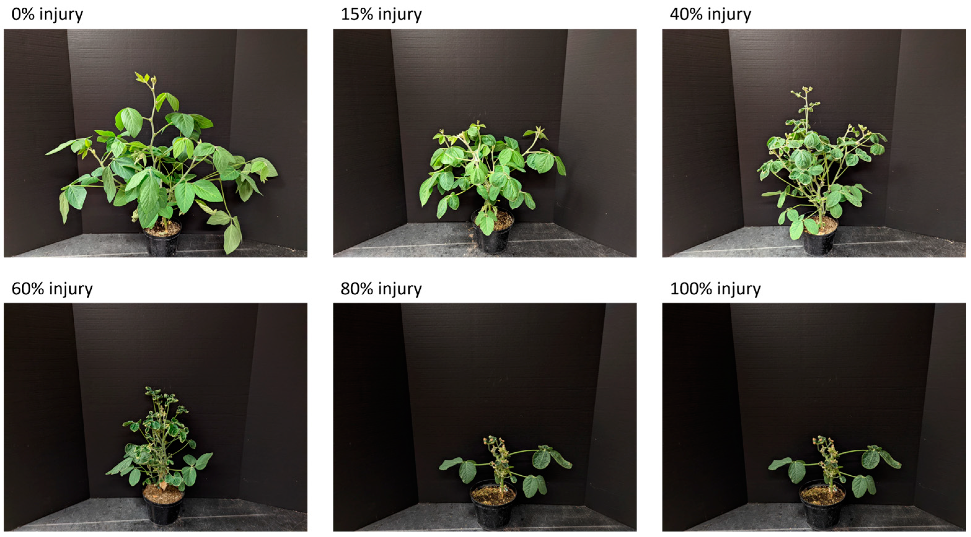
2.2. Image Acquisition and Visual Assessment of Herbicide Injury Phenotypes

LeafSpec, a leaf-scale hyperspectral imaging device developed by the Purdue Plant Phenotyping Lab, was used for image acquisition in this experiment. The device can fully scan a soybean leaf and acquire its hyperspectral data in a spectral range from 443 to 937 nm. The images have a resolution of 879 pixels for distribution analysis. The instrument was operated manually, and each scan took an average of 30 s. A fully unfolded leaflet of the 2nd trifoliate was imaged 1 to 2 HAT (hours after treatment) and 7, 14, 21, and 28 DAT (days after treatment). A fully unfolded leaflet of the youngest trifoliate of the plant was imaged at 8, 15, 22, and 29 DAT.
A visual assessment of damage was conducted at 7, 14, 21, and 28 DAT as validation of the herbicide treatment control. Damage was evaluated based on symptoms on the entire plant, including stem twisting, leaf drooping, leaf constriction, and formations of calloused tissue on the soybean stem [36] in a range from 0 (no damage symptoms) to 100 (dead plant) [37]. The assessment follows a standard in the field of weed science [16].
Photos of soybean plants with different damage levels are shown in Figure 1 as a reference.

2.3. Image Processing and Calibration

The segmentation between background and leaf samples in each hyperspectral image cube was based on a red-edge segmentation method [38,39]. The red-edge region referred to wavelengths between red color and the NIR region. Spectral reflectance of wavelengths at the red-edge was considered to be characteristic vegetation areas based on previous studies [40,41,42]. The wavelengths from 680 nm to 732 nm were selected as the red-edge region in this project. The algorithm is shown below:
l i n = t r a n s p o s e 20 : 20
c o n = l i n t r a n s p o s e ( s q u e e z e i m g : , : , I 680 : I 732 ) / ( l i n l i n )
p l t = c o n > t h r e s h o l d
A 1-dimensional (D) convolution kernel referred to as lin was used to convolve the red-edge region (Equation (1)) [43,44]. For optimal segmentation outcomes, a threshold of 7 was established according to Equation (3). Pixels that had values larger than the threshold were considered as leaf tissues and the rest of the pixels were considered as background.
After image segmentation, the hyperspectral images (HSIs) of leaf samples were calibrated with a white reference image taken with a flat strip of a white reference (a polyvinyl chloride (PVC) panel) [45,46,47]. The purpose of the white reference calibration was to reduce the noise from the uniformity of the light source for each wavelength [48]. The image calibration process was performed using the following equation:
R c a l i = R r a w R d a r k R w h i t e R d a r k
The spectral data were preprocessed with a Savitzky–Golay smoothing filter of order 1 with a window size of 5. The Savitzky–Golay smoothing filter is effective for noise reduction of spectra [49]. Image processing and analysis were carried out using MATLAB® 2020a (MathWorks Inc., Natick, MA, USA).

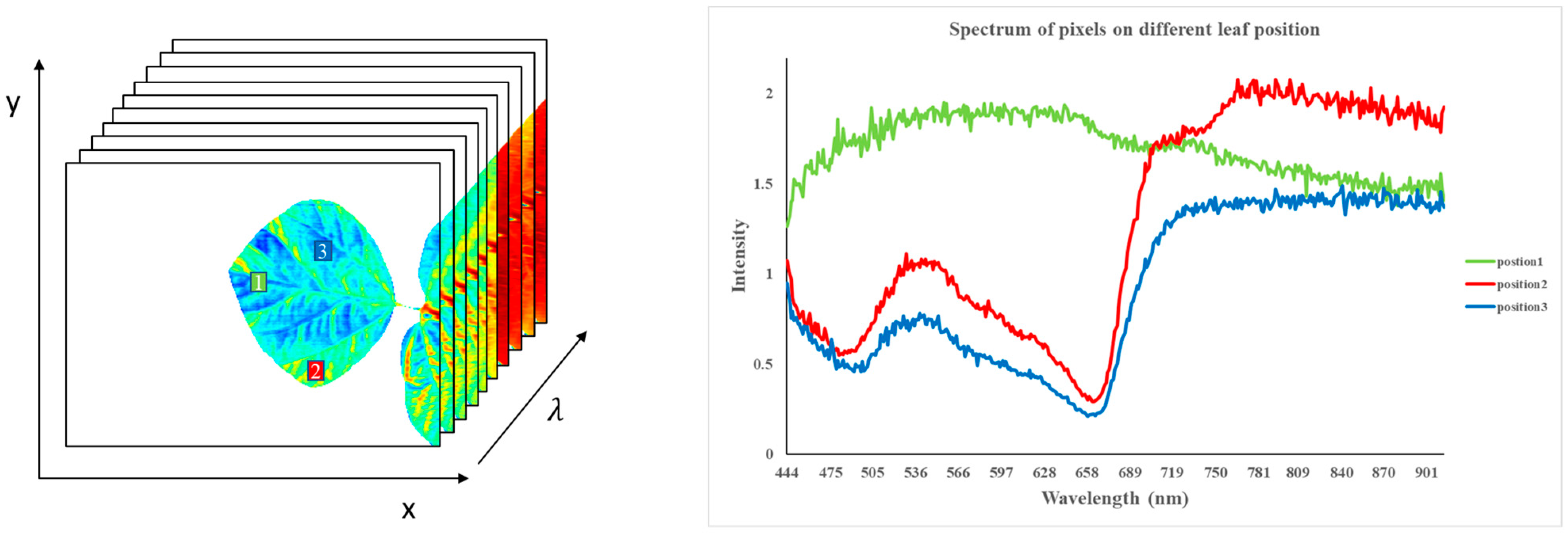
2.4. Mean Spectrum and Normalized Difference Vegetative Index (NDVI) Calculation from HSIs

The average spectrum of soybean leaves was obtained by averaging all the pixels of the entire leaf. This gave us an average spectrum of all experimental samples, covering spectral information from wavelengths of 443 nm to 937 nm. The two extreme ends of the spectrum were removed due to noise, and spectral data from 450 nm to 900 nm were used for further analysis. The NDVI was a useful tool for measuring leaf stress [23,40,43,50]. NDVI has also been proven to have a relationship with nitrogen status and chlorophyll [51]. Reflectance intensity at 800 nm and 630 nm were picked from the mean spectrum for NDVI calculations.

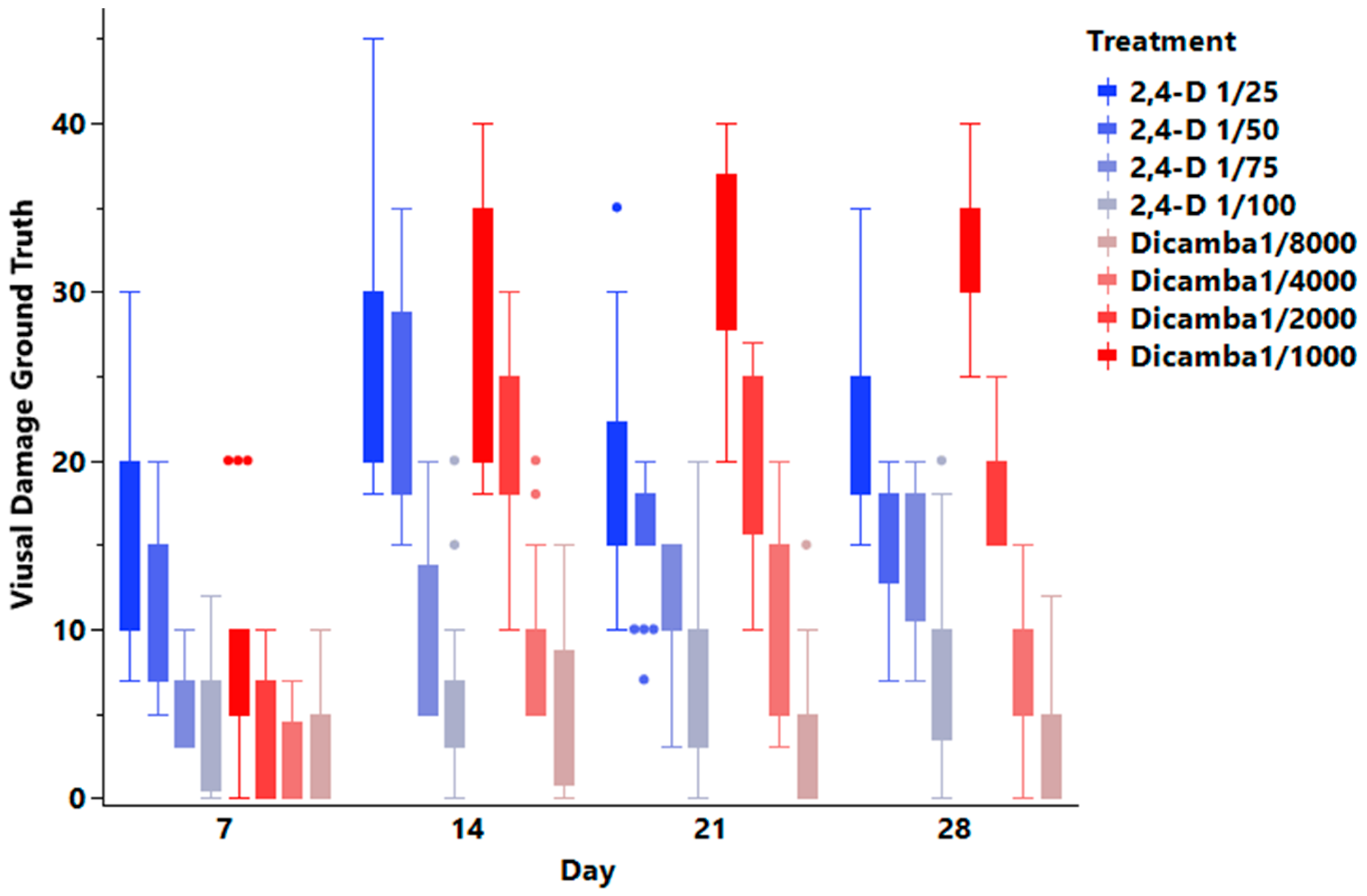
2.5. Statistical Tests for Visual Assessment of Herbicide Injuries and NDVI

The purpose of incorporating visual evaluation into the study was to confirm the efficacy of different dosages of our herbicide treatments. The NDVI was utilized to discern whether it could effectively differentiate between leaves treated with dicamba and 2,4-D. To evaluate the significance of the variations across different herbicide treatments, Tukey’s Honest Significance Difference (HSD) test was employed, with a significance level set at 0.05. This statistical method played a crucial role in pinpointing which treatment groups exhibited substantial differences [52], thereby offering a comprehensive insight into the effects of each treatment while mitigating the risk of Type I errors in multiple comparisons. Additionally, for each treatment group, the mean and standard deviation were calculated to provide a detailed statistical representation.
All statistical analyses were conducted using JMP software (Version 16, SAS Institute Inc., Cary, NC, USA), a robust and widely recognized statistical package. The use of this software not only ensures the credibility and accuracy of our statistical analysis but also enhances the reproducibility and scientific rigor of our study.

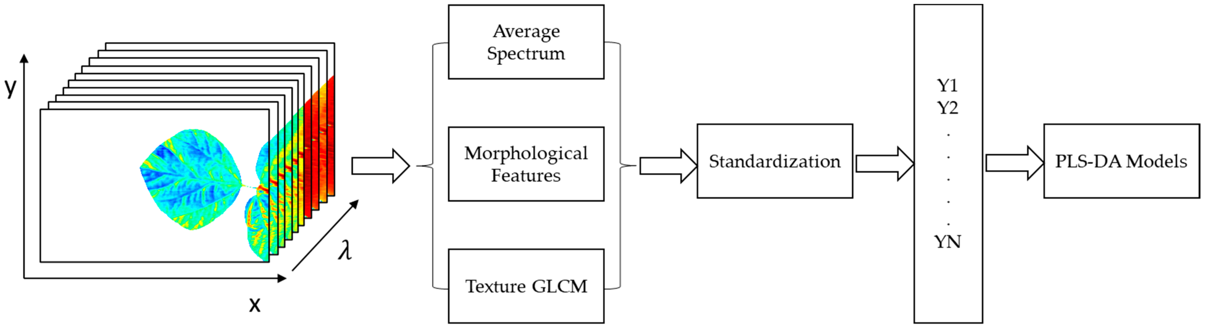
2.6. Machine Learning Classification Model Built by Leaf Average Spectrum

A pairwise partial least squares discriminant analysis (PLS-DA) algorithm and a Mahalanobis distance-based nearest neighbor method was applied to the mean spectral data of the fully unfolded leaflet of the 2nd trifoliate. PLS-DA is a machine learning classification algorithm suitable for high-dimensional data [53,54,55]. PLS-DA can extract high-dimensional X data into low-dimensional Y space [56]. The algorithm has been proven to be effective in processing hyperspectral data [43,53,54] The algorithm was applied to the processed averaged spectra through the PLS_Toolbox (Version 8.8, Eigenvector Research, Inc. Manson, WA, USA), which is one suite of multivariate and machine learning tools within the MATLAB® computational environment. A single PLS-DA model is a binary classification model. For a classification task with multiple classes, pairwise binary models are created by forming all two-by-two combinations between all classes. By voting all binary prediction results, the model is able to provide a prediction result for the multi-class classification. The nearest neighbor algorithm was employed, utilizing the Mahalanobis distance as the distance metric for the development of classification models. The Mahalanobis distance (M-distance) was selected as it accounts for the variance within the data and is adept at identifying similarities in high-dimensional spaces [57,58]. The calculation for the M-distance is shown in Equation (2). D indicates the M-distance, x is the spectra data by wavelength, m is the mean of each band for a group of spectrum, and C 1 stands for the inverse covariance matrix of the independent variables.
D 2 = x m T · C 1 · ( x m )
We divided the data into three different datasets, each containing data for 1, 7, 14, 21, and 28 DAT, and the specific information of the data set is shown in Table 2.
Given that visual symptoms typically manifest 14 days after treatment (DAT), the dataset corresponding to this time frame was chosen as a preliminary set for comparing the performance of the PLS-DA and M-distance. The method demonstrating superior performance in this initial comparison was subsequently selected as the preferred modeling approach for datasets encompassing all observation days. In training each model, mean-centered and auto-scaled methods were chosen to pre-process the original spectra. The number of latent variables for each PLS-DA model was set to 3. The leave-one-out cross-validation method was used for the model to determine the prediction accuracy. In the classifier employing the M-distance, the computation involved determining the distance between each test spectrum and all spectra within the treatment groups, excluding the one being tested. The treatment group that displayed the shortest distance to the test spectrum was identified and subsequently selected as the classifier’s output. Overall Accuracy (OA) and error rate were used to examine the performance of models. They were calculated using Equation (6):
O A = N u m b r   o f   C o r r e c t   P r e d i c t i o n s T o t a l   N u m b e r   o f   P r e d i c t i o n s
The study also attempted to visualize the prediction results of the PLS-DA model and explore the spatial information by applying the model to each pixel of the hyperspectral image. Heatmaps were created showing the prediction results of the soft voting probability of the control treatment at different locations of the leaf image.

2.7. Distribution Analysis of Herbicide Injury Classification on Top Matured Leaves

To better capture the damage signal of herbicides on soybean leaves using hyperspectral images, this project conducted a distribution analysis with spatial information, highlighting the need for spatial analysis. As shown in Figure 2, the high-resolution hyperspectral images show clear differences in spectral information across different locations, further emphasizing the limitations of the average spectrum method.
A spatial distribution analysis can extract leaf damage features such as leaf scars and abnormal shape growth. Since the symptoms of damage are usually observed on newly grown leaves [12,13], images of top matured leaves were used for the leaf-level spatial distribution study. Morphological and texture features were calculated from HSIs as key information of leaf spatial distribution. Combining this with the mean spectrum data extracted from previous steps of the same plant, a new dataset containing both spatial and spectral information was created to train the herbicide classification models. The trained model aimed to achieve better performance in classifying different herbicide dosages. The number of latent variables was set to 5 in this modeling process. A performance comparison was made between classification based on spectrum only and the combination of spectrum, morphological, and texture features. The layout of the modeling process is shown in Figure 3.

2.7.1. Morphological Features

The binary masks generated from the segmented images were used to extract the morphological features of soybean leaves. The morphological features were obtained by applying the regionprops function in MATLAB (Version 2021a, MathWorks, Natick, MA, USA). In this research, leaf area, convex area, eccentricity, major axis length, minor axis length, and solidity were included as morphological features. The detailed equations for the above features extraction are presented in the MATLAB official documentation [52].

2.7.2. Texture Analysis

The Gray-Level Co-Occurrence Matrix (GLCM) is a statistical algorithm for extracting texture information. The GLCM functions characterize the texture of an image by calculating how often pairs of pixels with certain values and in a specified spatial relationship occur in an image, creating a GLCM, and then extracting statistical measures from this matrix [59,60]. In this study, contrast, correlation, energy, and homogeneity were calculated as texture features by using MATLAB. These GLCM measurements were found to be useful in identifying the spatial feature of plant leaves [61,62].
In this experiment, the sample images were first cropped to ensure that they were the same size. The cropped images were inspected with the human eye to ensure that only plant tissue information was included. Since the algorithm could only compute single-channel matrices, it was necessary to reduce the dimensionality of the hyperspectral data. A total of 386 bands were divided into 50 bands by calculating the average value. Texture features were calculated for each binned band; 200 texture features were selected for each HSI in total.

3. Results and Discussion

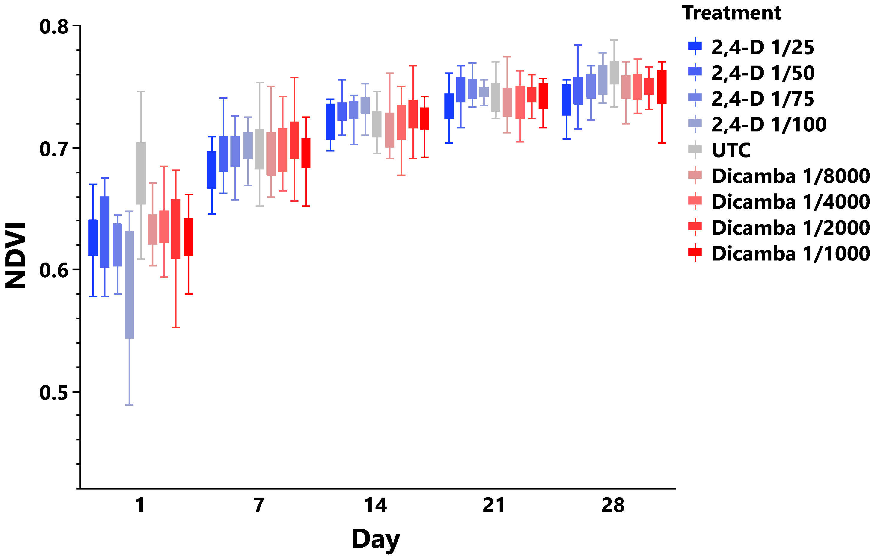
3.1. Visual Damage Ground Truth and NDVI

The visual damage assessment showed that the severity of the damage to the soybean plants increased with the concentration of the herbicide applied (Figure 4). The 2,4-D groups exhibited the most severe damage at 14 days after herbicide spray treatment (14 DAT), with damage symptoms decreasing after this time point. In contrast, soybean injuries caused by dicamba increased with both the herbicide dose and time after treatment. However, the visual injury evaluation alone could not distinguish between dicamba and 2,4-D (Table 3).
Table 3 presents the comparison of average visual damage ratings for each herbicide treatment at 7, 14, 21, and 28 days after spraying. The data are organized by treatment, with mean visual injury scores and standard deviations provided for each time point. The visual injury was assessed on a scale of 0 to 100%, with 0 representing no visible injury and 100% representing complete plant death. Means followed by the same letter within a column are not significantly different according to Tukey’s honest significant difference (HSD) test results (α level of 0.05).
The NDVI values increased over time, demonstrating a growth trend of the plants over the 28 days after treatment (DAT) (Figure 5). Significant differences were observed between the NDVI values of the untreated control and herbicide-treated plants across all evaluation time points (Table 4). However, except for 1 DAT, the differences in NDVI values between the various herbicide treatments were not significant. The mean ± error and the results of Tukey’s honest significant difference (HSD) test are presented in Table 3.

3.2. Machine Learning Classification Modeling Result of Mean Spectrum of the Whole Leaf

3.2.1. Machine Learning Method Comparison Preliminary Result

In the evaluation of machine learning models using the 14 DAT dataset, the results in Table 5 revealed distinct differences in performance between the M-distance and PLS-DA models. For the high-dosage-only dataset, the M-distance model achieved an OA of 86.67%, while the PLS-DA model demonstrated a superior performance with an OA of 93.3%. In the combined-dosages dataset, the M-distance model’s accuracy decreased to 63.33%, whereas the PLS-DA model maintained a higher accuracy level of 86.1%. The most comprehensive dataset, encompassing all treatments, saw a further decline in the accuracy of the M-distance model to 31.11%, while the PLS-DA model achieved an OA of 57.4%. These results indicate the enhanced capability of the PLS-DA model in handling varied herbicide dosages and complex treatment scenarios compared to the M-distance model.

3.2.2. High-Dosage Herbicide Treatment Classification

To test the feasibility of the mean spectrum, the two herbicide treatment groups with the highest concentrations and the untreated control group were selected to build pairwise PLS-DA models. The overall accuracy of the model exceeded 90% from the 1 DAT data. The untreated control group achieved a 95% classification accuracy with the 1 DAT data (Table 6). As the herbicide damage signal gradually intensified, the accuracy of the model also increased. The overall accuracy of the PLS-DA model rose from 91.8% to 98.33% after 28 days (Table 6).

3.2.3. Combined Dosages Dataset Classification

The overall accuracy of models built on hyperspectral data collection on each evaluation time point was close to or higher than 80% (Table 7). Models built from 7 and 28 DAT data had the highest accuracy across all evaluation days. The untreated control group was classified with 95% accuracy on the very first day after treatment (1 DAT). The classification rate of combined dosages of dicamba increased over time and achieved an accuracy of 93.8% on 28 DAT. However, the accuracy of combined dosages of 2,4-D dropped from 14 to 28 DAT.

3.2.4. All Treatments Dataset Classification

Table 8 displays the classification results of the PLS-DA models built for all herbicide treatments and the untreated control using average spectrum data on 1, 7, 14, 21, and 28 DAT. The control group was classified with over 80% accuracy for each evaluation day. For each herbicide treatment, the classification accuracy was over 65% on at least one of the five evaluation time points. For the 2,4-D treatments, the highest and lowest dosages had an overall accuracy of more than 75%. For the dicamba treatments, lower dosages (1/4000 and 1/8000) had better classification results than higher dosages.

3.2.5. PLS-DA Prediction Result Heatmap

The heatmap in Figure 6 shows that the values of the pixel points at different positions of the leaf did not completely coincide. Some spatial distribution patterns of the different herbicide treatments were observed, such as the texture information of the leaves (e.g., veins) and differences in pixel values between dicamba, 2,4-D, and the untreated control on the veins and the dots around the veins. Figure 7 reveals coherence in the dicamba group heatmap, with clearly visible red regions.

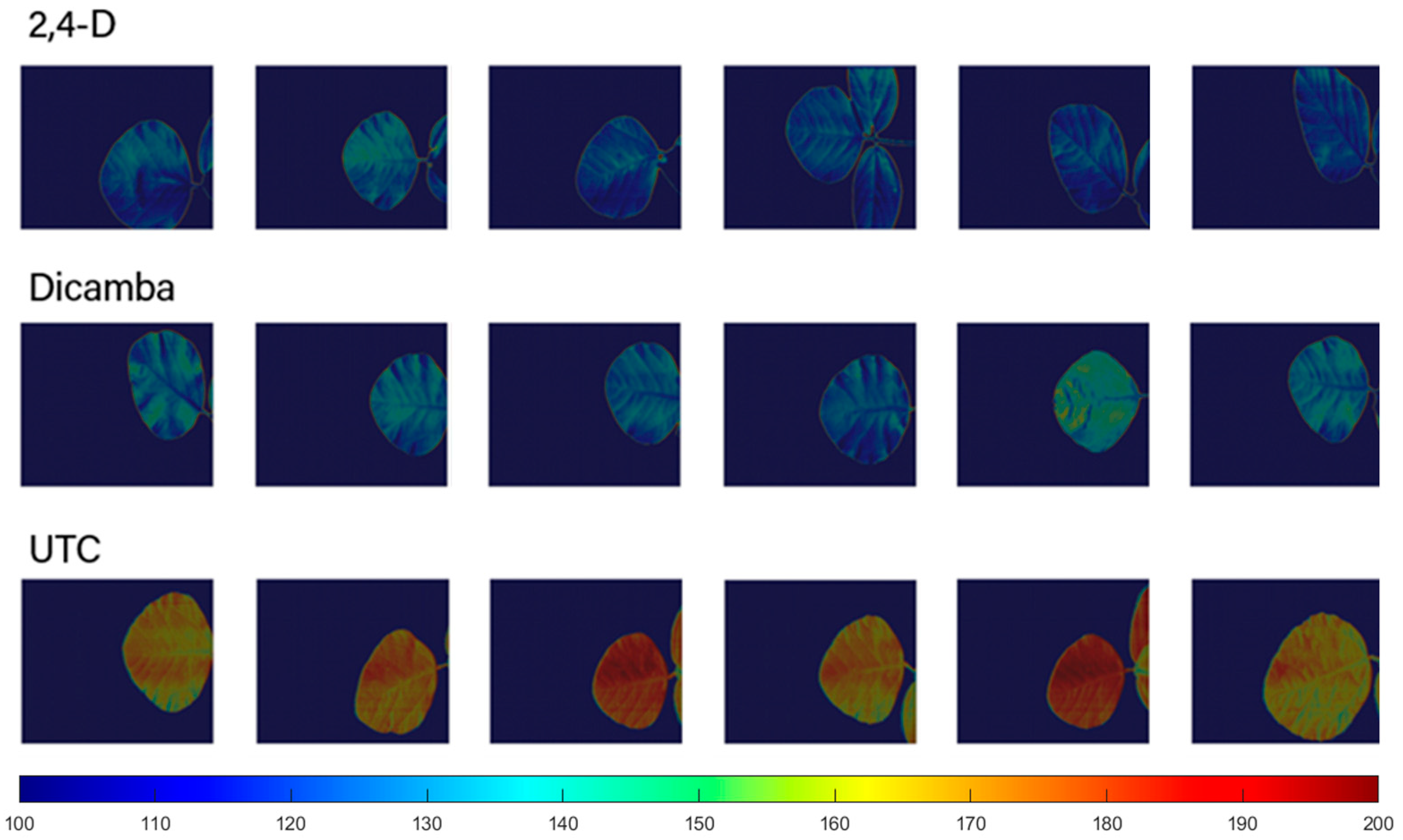
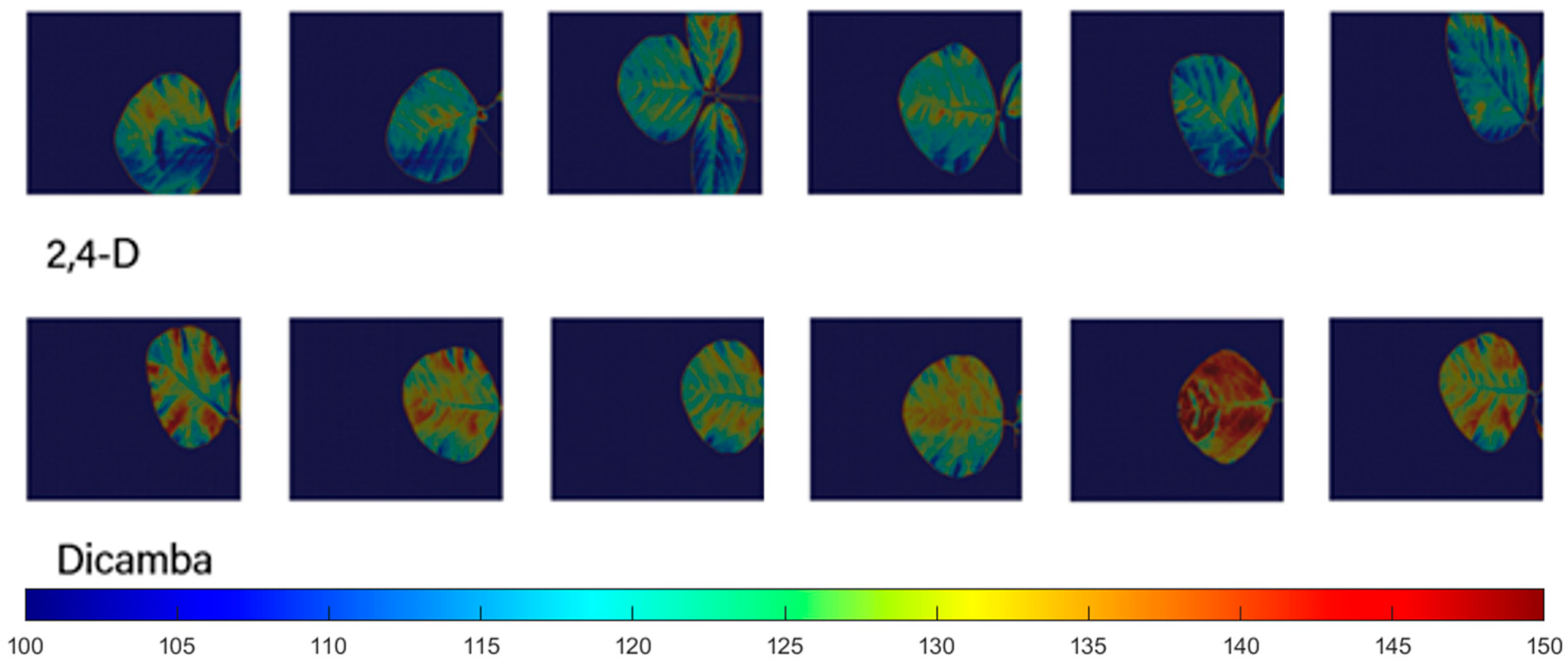
3.3. Distribution Analysis Result of Dicamba and 2,4-D Damage

The classification accuracy increased significantly after texture and morphological features were added to the training dataset (Table 9). This suggests that the spatial analysis contributes important features that reflect the varying magnitude of responses to different herbicide doses. The 14 DAT dataset had the highest overall classification accuracy, which is consistent with the results of the visual evaluation.

4. Discussion

4.1. Visual Damage Ground Truth and NDVI

These results demonstrate the similarities in damage caused by dicamba and 2,4-D for each dosage level, indicating that the experiment was well-controlled and prepared and the protocol can be applied for future classification methods. The decrease in damage symptoms for the 2,4-D groups after 14 DAT is consistent with previous research [33]. Soybean injury from dicamba, on the other hand, increased with both the increasing herbicide dose and time after treatment, as reported by Robinson et al. (2013) [16,33]. Given the visual similarities between the damage caused by dicamba and 2,4-D, it is essential to develop more advanced methods to differentiate between the two.
The NDVI values were found to increase over time, illustrating the growth trend of the plants over 28 DAT. This is because NDVI values tend to increase as plants grow and develop more leaves and chlorophyll. Soybean plants, which absorb red light for photosynthesis and reflect near-infrared light, have higher NDVI values [23,63]. Another finding is that significant differences were found between herbicides with different dosages at the earliest time point (2 HAT), and the differences in NDVI decreased over time. This observation aligns with the results of Huang et al. (2016), which also highlighted that the accuracy of detection decreases at later stages (2 weeks after treatment or WAT), particularly at higher doses [23].
The results of the NDVI analysis indicated that the mean NDVI method was insufficient to distinguish between different dosages of dicamba and 2,4-D herbicides. Although there was a significant difference between the NDVI values of untreated control and herbicide-treated plants, the differences between herbicide treatments were not significant. The limitation of NDVI may be attributed to its averaging effect across the entire leaf, potentially leading to a dilution effect. Furthermore, dicamba and 2,4-D use the same herbicide mode of action as plant growth regulators [26], suggesting a high degree of similarity in their spectral effects. This similarity posits that a single Vegetation Index (VI) may be inadequate for discerning their differences [43]. Consequently, the employment of more sophisticated machine learning algorithms, such as PLS-DA, which can leverage spectral information across all wavelengths, becomes imperative. Additionally, a spatial analysis capable of extracting signals related to leaf malformation is essential for the advancement of this research. This approach could provide a more nuanced understanding of the herbicidal impacts, thereby enhancing the efficacy of plant phenotyping studies. The study aimed to address this need by combining spectral and spatial information to better detect and distinguish the herbicide-induced damage on soybean plants.

4.2. Machine Learning Classification Result of Mean Spectrum of the Whole Leaf

4.2.1. High-Dosage Herbicide Treatment Classification

This study found that the model developed using hyperspectral data was able to detect differences in herbicide treatments earlier than the human eye could. This is because soybean injury from even low doses of dicamba may not be visible until 14 DAT [34]. In this particular study, no visual damage was observed at 2 HAT, and only a low level of damage was observed at 7 DAT. Furthermore, the accuracy of classification in the untreated control group suggests that the herbicide signal can be detected by the model built on LeafSpec hyperspectral data.
One possible explanation for this is that soybeans experience a stress response to the newly exposed herbicide, resulting in subtle changes in the leaves that are imperceptible to the human eye but can be captured by hyperspectral information. It was hypothesized that in the early stages of exposure, there are strong signals in the near-infrared region. This explains why using NDVI can detect damage that is imperceptible to the human eye [23].
The increase in the model’s accuracy over time, as the herbicide damage signal gradually intensified, indicates that the herbicides continuously affected soybean plants and that the damage caused by the herbicides did not diminish over time. This finding is consistent with the information from the visual assessment of the herbicide-induced damage [16,64]. The high classification accuracy achieved by the models highlights the potential of hyperspectral data for detecting and differentiating herbicide damage in soybean plants.

4.2.2. Combined Dosages Dataset Classification

The trend of herbicide treatment accuracy could be explained by the visual assessment of herbicide damage. The results of the combined dosage model proved that the PLS-DA models based on mean spectra were able to capture the signal of different dosages of dicamba and 2,4-D applied on soybean leaves. The high classification rate for the dicamba and 2,4-D treatments suggests that soybean plants respond differently to the two herbicides, and also demonstrated that PLS-DA models built upon high-dimensional spectral data were able to capture this difference.
The decrease in accuracy of the combined-dosage 2,4-D model from day 14 to 28 DAT can be attributed to the decline in visual damage observed in our research. As the symptoms of 2,4-D injury diminished over time, it became more challenging for the PLS-DA model to accurately classify the herbicide-treated plants. This highlights the importance of considering the temporal dynamics of herbicide-induced damages when developing classification models based on hyperspectral data.

4.2.3. All Treatments Dataset Classification

These results suggest that the spectral information of leaves can reflect how soybean responds differently to different doses of herbicide. However, the signals captured by the model were not able to distinguish these differences very accurately. This implies that the average spectral modeling approach is not sufficient to solve this problem. To improve the performance of the model, future studies should consider introducing a leaf distribution analysis. By incorporating spatial information and potentially more sophisticated classification algorithms, the ability to accurately distinguish between different herbicide treatments may be enhanced.

4.3. Distribution Analysis Result of Dicamba and 2,4-D Damage

The integration of texture and morphological features into the PLS-DA model not only enriches the dataset but also introduces a multi-dimensional approach to plant phenotyping, particularly in the context of herbicide damage assessment. This approach transcends the limitations of traditional spectral analyses, which, while effective, often overlook the spatial and textural nuances that are crucial in understanding the full impact of herbicides like dicamba and 2,4-D. Texture features, which describe the surface characteristics of leaves, provide valuable insights into the subtle changes caused by herbicides that might not be discernible through a spectral analysis alone. These features can capture variations in leaf surface smoothness, roughness, or pattern changes, which are indicative of herbicidal effects. By incorporating these texture characteristics, the model gains a deeper layer of data, enhancing its ability to detect and classify the nuanced effects of different herbicides on plant leaves. Similarly, morphological features, which involve the shape and structural attributes of leaves, play a crucial role in assessing herbicide impact. Herbicides, especially growth regulators like dicamba and 2,4-D, often cause deformities in leaf shape, such as curling, twisting, or abnormal growth patterns. By quantifying these changes, the model becomes more adept at identifying the specific herbicide responsible for the damage. This is particularly significant in distinguishing between herbicides that might have similar spectral signatures but different morphological impacts on plants.
The inclusion of these features represents a significant advancement in plant phenotyping, particularly in the realm of precision agriculture. By employing a more holistic view of plant responses to herbicides, it becomes possible to achieve more accurate and comprehensive assessments. This is crucial not only for understanding the effects of specific herbicides but also for developing more effective and sustainable agricultural practices.
In future work, it is crucial to recognize that the current approach combining GLCM with image processing for feature extraction and PLS-DA modeling is an initial effort to use both spatial and spectral data. Although promising, this method is still being developed. Advancements in machine learning, especially neural networks, offer potential enhancements. Neural networks, particularly deep learning models, are adept at handling complex spatial and spectral data, which is crucial for plant phenotyping. Looking forward, the application of such an enhanced model in remote sensing, especially through high-resolution imaging from drones, opens up new frontiers in large-scale agricultural monitoring. The ability to detect herbicide damage at the canopy level using drones equipped with advanced imaging technology would revolutionize the way we monitor and manage crop health on a large scale. It would enable the early detection of herbicide stress, allowing for timely interventions to mitigate damage. Furthermore, this technology could be pivotal in precision agriculture, where site-specific management practices are employed to optimize crop health and yield.

5. Conclusions

This study demonstrated the potential of a high-precision spatial and spectral imaging solution for the early detection and classification of soybean damage caused by dicamba and 2,4-D herbicides. By combining spectral and spatial features, the classification accuracy of herbicide treatments and dosages was significantly improved compared to using spectral data alone or traditional human inspection. The novel touch-based leaf imager, LeafSpec, provided high-resolution imaging with a high signal-to-noise ratio, enabling a more accurate herbicide damage diagnosis. This study achieved two significant breakthroughs in using hyperspectral plant phenotyping to study herbicide-induced damage to soybeans, specifically for extremely low concentrations of dicamba and 2,4-D. In our experiments, the model was capable of detecting damage from dicamba at a dilution as low as 1:8000 and from 2,4-D at a dilution of 1:75.
Advanced machine learning models, such as pairwise PLS-DA models, were employed to enhance the accuracy of the detection results by incorporating spectral information, leaf color distribution, texture, and morphological features. These methods have the potential to advance imaging technologies for plant diagnostic labs and state regulatory agencies, helping to determine the source and liability responsibilities of herbicide off-target damage.
Future research is expected to concentrate on advancing methods that combine spatial and spectral analyses for practical applications in herbicide drift detection models. Furthermore, attention will be directed towards evaluating the transferability of models from greenhouse settings to real-world agricultural environments. In the pursuit of this goal, efforts are being made to integrate the model into an unmanned aerial vehicle (UAV) field scouting robot, a move that resonates with the overarching theme of remote sensing. This integration is envisioned to facilitate large-scale, real-time monitoring and assessment of herbicide damage in agricultural landscapes. To verify the effectiveness of these methods, field trials are being planned for execution.

Author Contributions

Conceptualization, Z.N., J.Y., X.W. and J.J.; methodology, Z.N. and J.J.; software, Z.N.; validation, Z.N.; formal analysis, Z.N.; data curation, Z.N.; writing—original draft preparation, Z.N.; writing—review and editing, J.Y., X.W., J.J., W.G.J. and B.Y.; visualization, Z.N.; supervision, J.J.; project administration, J.J.; funding acquisition, J.J. All authors have read and agreed to the published version of the manuscript.

Funding

This research received no external funding.

Data Availability Statement

The data presented in this study are available on request from the corresponding author. The data are not publicly available due to confidentiality.

Acknowledgments

The authors would like to thank Libo Zhang (postdoc, Department of Agronomy, Purdue University), Ziling Chen (graduate student, Department of Agriculture and Biological Engineering, Purdue University) for their assistance during the plant cultivation and imaging data collection.

Conflicts of Interest

The authors declare no conflict of interest.

References

  1. Meyeres, T.; Lancaster, S.; Kumar, V.; Roozeboom, K.; Peterson, D. Non-Dicamba-Resistant Soybean Response to Multiple Dicamba Applications. Agron. J. 2023, 115, 147–160. [Google Scholar] [CrossRef]
  2. Riter, L.S.; Pai, N.; Vieira, B.C.; MacInnes, A.; Reiss, R.; Hapeman, C.J.; Kruger, G.R. Conversations about the Future of Dicamba: The Science Behind Off-Target Movement. J. Agric. Food Chem. 2021, 69, 14435–14444. [Google Scholar] [CrossRef] [PubMed]
  3. Behrens, M.R.; Mutlu, N.; Chakraborty, S.; Dumitru, R.; Jiang, W.Z.; LaVallee, B.J.; Herman, P.L.; Clemente, T.E.; Weeks, D.P. Dicamba Resistance: Enlarging and Preserving Biotechnology-Based Weed Management Strategies. Science 2007, 316, 1185–1188. [Google Scholar] [CrossRef] [PubMed]
  4. Byker, H.P.; Soltani, N.; Robinson, D.E.; Tardif, F.J.; Lawton, M.B.; Sikkema, P.H. Control of Glyphosate-Resistant Horseweed (Conyza canadensis) with Dicamba Applied Preplant and Postemergence in Dicamba-Resistant Soybean. Weed Technol. 2013, 27, 492–496. [Google Scholar] [CrossRef]
  5. Hodgskiss, C.; Legleiter, T.; Young, B.; Johnson, W. Effects of Herbicide Management Practices on the Weed Density and Richness in 2,4-D-Resistant Cropping Systems in Indiana. Weed Technol. 2021, 36, 130–136. [Google Scholar] [CrossRef]
  6. Peterson, M.A.; McMaster, S.A.; Riechers, D.E.; Skelton, J.; Stahlman, P.W. 2,4-D Past, Present, and Future: A Review. Weed Technol. 2016, 30, 303–345. [Google Scholar] [CrossRef]
  7. Islam, F.; Wang, J.; Farooq, M.A.; Khan, M.S.S.; Xu, L.; Zhu, J.; Zhao, M.; Muños, S.; Li, Q.X.; Zhou, W. Potential Impact of the Herbicide 2,4-Dichlorophenoxyacetic Acid on Human and Ecosystems. Environ. Int. 2018, 111, 332–351. [Google Scholar] [CrossRef] [PubMed]
  8. Brochado, M.G.d.S.; Mielke, K.C.; de Paula, D.F.; Laube, A.F.S.; Alcántara-de la Cruz, R.; Gonzatto, M.P.; Mendes, K.F. Impacts of Dicamba and 2,4-D Drift on ‘Ponkan’ Mandarin Seedlings, Soil Microbiota and Amaranthus Retroflexus. J. Hazard. Mater. Adv. 2022, 6, 100084. [Google Scholar] [CrossRef]
  9. Ceolin, B.C.; Kemmerich, M.; Noguera, M.M.; Camargo, E.R.; Avila, L.A. de Evaluation of an Alternative Sorbent for Passive Sampling of the Herbicides 2,4-D and Dicamba in the Air. J. Environ. Sci. Health Part B 2021, 56, 634–643. [Google Scholar] [CrossRef]
  10. Egan, J.F.; Mortensen, D.A. Quantifying Vapor Drift of Dicamba Herbicides Applied to Soybean. Environ. Toxicol. Chem. 2012, 31, 1023–1031. [Google Scholar] [CrossRef]
  11. Osipitan, O.A.; Scott, J.E.; Knezevic, S.Z. Glyphosate-Resistant Soybean Response to Micro-Rates of Three Dicamba-Based Herbicides. Agrosyst. Geosci. Environ. 2019, 2, 180052. [Google Scholar] [CrossRef]
  12. Jones, G.T.; Norsworthy, J.K.; Barber, T.; Gbur, E.; Kruger, G.R. Off-Target Movement of DGA and BAPMA Dicamba to Sensitive Soybean. Weed Technol. 2019, 33, 51–65. [Google Scholar] [CrossRef]
  13. Soltani, N.; Oliveira, M.C.; Alves, G.S.; Werle, R.; Norsworthy, J.K.; Sprague, C.L.; Young, B.G.; Reynolds, D.B.; Brown, A.; Sikkema, P.H. Off-Target Movement Assessment of Dicamba in North America. Weed Technol. 2020, 34, 318–330. [Google Scholar] [CrossRef]
  14. Bish, M.D.; Bradley, K.W. Survey of Missouri Pesticide Applicator Practices, Knowledge, and Perceptions. Weed Technol. 2017, 31, 165–177. [Google Scholar] [CrossRef]
  15. Erickson, B.E. Dicamba Still Harmed Nontarget Crops in 2021. Chem. Eng. News 2022, 100, 19. [Google Scholar] [CrossRef]
  16. Robinson, A.P.; Simpson, D.M.; Johnson, W.G. Response of Glyphosate-Tolerant Soybean Yield Components to Dicamba Exposure. Weed Sci. 2013, 61, 526–536. [Google Scholar] [CrossRef]
  17. Scholtes, A.B.; Sperry, B.P.; Reynolds, D.B.; Irby, J.T.; Eubank, T.W.; Barber, L.T.; Dodds, D.M. Effect of Soybean Growth Stage on Sensitivity to Sublethal Rates of Dicamba and 2,4-D. Weed Technol. 2019, 33, 555–561. [Google Scholar] [CrossRef]
  18. Centner, T.J. Creating a Compensation Program for Injuries from Dicamba Spray Drift and Volatilization. Appl. Econ. Perspect. Policy 2022, 44, 1068–1082. [Google Scholar] [CrossRef]
  19. González, A.J.; Gallego, A.; Gemini, V.L.; Papalia, M.; Radice, M.; Gutkind, G.; Planes, E.; Korol, S.E. Degradation and Detoxification of the Herbicide 2,4-Dichlorophenoxyacetic Acid (2,4-D) by an Indigenous Delftia Sp. Strain in Batch and Continuous Systems. Int. Biodeterior. Biodegrad. 2012, 66, 8–13. [Google Scholar] [CrossRef]
  20. Foster, M.R.; Griffin, J.L. Injury Criteria Associated with Soybean Exposure to Dicamba. Weed Technol. 2018, 32, 608–617. [Google Scholar] [CrossRef]
  21. Shi, C.; Zheng, Y.; Geng, J.; Liu, C.; Pei, H.; Ren, Y.; Dong, Z.; Zhao, L.; Zhang, N.; Chen, F. Identification of Herbicide Resistance Loci Using a Genome-Wide Association Study and Linkage Mapping in Chinese Common Wheat. Crop J. 2020, 8, 666–675. [Google Scholar] [CrossRef]
  22. Herbicide Damage to Plants. Available online: https://www.missouribotanicalgarden.org/gardens-gardening/your-garden/help-for-the-home-gardener/advice-tips-resources/pests-and-problems/environmental/herbicide (accessed on 7 January 2023).
  23. Huang, Y.; Yuan, L.; Reddy, K.N.; Zhang, J. In-Situ Plant Hyperspectral Sensing for Early Detection of Soybean Injury from Dicamba. Biosyst. Eng. 2016, 149, 51–59. [Google Scholar] [CrossRef]
  24. Suarez, L.A.; Apan, A.; Werth, J. Detection of Phenoxy Herbicide Dosage in Cotton Crops through the Analysis of Hyperspectral Data. Int. J. Remote Sens. 2017, 38, 6528–6553. [Google Scholar] [CrossRef]
  25. Marques, M.G.; da Cunha, J.P.A.R.; Lemes, E.M. Dicamba Injury on Soybean Assessed Visually and with Spectral Vegetation Index. AgriEngineering 2021, 3, 240–250. [Google Scholar] [CrossRef]
  26. Sherwani, S.I.; Arif, I.A.; Khan, H.A.; Sherwani, S.I.; Arif, I.A.; Khan, H.A. Modes of Action of Different Classes of Herbicides. In Herbicides, Physiology of Action, and Safety; IntechOpen: London, UK, 2015; ISBN 978-953-51-2217-3. [Google Scholar]
  27. Ma, D.; Wang, L.; Zhang, L.; Song, Z.; Rehman, T.U.; Jin, J. Stress Distribution Analysis on Hyperspectral Corn Leaf Images for Improved Phenotyping Quality. Sensors 2020, 20, 3659. [Google Scholar] [CrossRef] [PubMed]
  28. Ge, Y.; Bai, G.; Stoerger, V.; Schnable, J.C. Temporal Dynamics of Maize Plant Growth, Water Use, and Leaf Water Content Using Automated High Throughput RGB and Hyperspectral Imaging. Comput. Electron. Agric. 2016, 127, 625–632. [Google Scholar] [CrossRef]
  29. McFadden, D.; Fry, J.; Keeley, S.; Hoyle, J.; Raudenbush, Z. Establishment of Kentucky Bluegrass and Tall Fescue Seeded after Herbicide Application. Crop Forage Turfgrass Manag. 2022, 8, e20151. [Google Scholar] [CrossRef]
  30. Hu, J.; Li, C.; Wen, Y.; Gao, X.; Shi, F.; Han, L. Spatial Distribution of SPAD Value and Determination of the Suitable Leaf for N Diagnosis in Cucumber. IOP Conf. Ser. Earth Environ. Sci. 2018, 108, 022001. [Google Scholar] [CrossRef]
  31. Weidenhamer, J.D.; Triplett, G.B., Jr.; Sobotka, F.E. Dicamba Injury to Soybean. Agron. J. 1989, 81, 637–643. [Google Scholar] [CrossRef]
  32. Roesler, G.D.; Jonck, L.C.G.; Silva, R.P.; Victoria, J.A.; Silva, H.A.C.; Monquero, P.A. Decontamination Methods of Tanks to Spray 2,4-D and Dicamba and the Effects of These Herbicides on Citrus and Vegetable Species. Aust. J. Crop Sci. 2020, 14, 1302–1309. [Google Scholar] [CrossRef]
  33. Wang, L.; Duan, Y.; Zhang, L.; Wang, J.; Li, Y.; Jin, J. LeafScope: A Portable High-Resolution Multispectral Imager for In Vivo Imaging Soybean Leaf. Sensors 2020, 20, 2194. [Google Scholar] [CrossRef] [PubMed]
  34. Yogeshwari, M.; Thailambal, G. Automatic Feature Extraction and Detection of Plant Leaf Disease Using GLCM Features and Convolutional Neural Networks. Mater. Today Proc. 2023, 81, 530–536. [Google Scholar] [CrossRef]
  35. Mahajan, S.; Raina, A.; Gao, X.-Z.; Kant Pandit, A. Plant Recognition Using Morphological Feature Extraction and Transfer Learning over SVM and AdaBoost. Symmetry 2021, 13, 356. [Google Scholar] [CrossRef]
  36. Zimmer, M. Differentiating 2,4-D and Dicamba Injury on Soybeans; Purdue University: West Lafayette, IN, USA, 2019. [Google Scholar]
  37. Behrens, R.; Lueschen, W.E. Dicamba Volatility. Weed Sci. 1979, 27, 486–493. [Google Scholar] [CrossRef]
  38. Zhang, L.; Maki, H.; Ma, D.; Sánchez-Gallego, J.A.; Mickelbart, M.V.; Wang, L.; Rehman, T.U.; Jin, J. Optimized Angles of the Swing Hyperspectral Imaging System for Single Corn Plant. Comput. Electron. Agric. 2019, 156, 349–359. [Google Scholar] [CrossRef]
  39. Li, T.; Li, J.; Xiao, J.; Liu, X.; Tang, H. Man-Made Target Detection Method Based on the Red-Edge Spectral Information in Natural Background. In Proceedings of the AOPC 2022: Optical Sensing, Imaging, and Display Technology, Beijing, China, 18–20 December 2022; SPIE: Bellingham, WA, USA, 2023; Volume 12557, pp. 507–513. [Google Scholar]
  40. Collins, W. Remote Sensing of Crop Type and Maturity. Photogramm. Eng. Remote Sens. 1978, 44, 43–55. [Google Scholar]
  41. Le Bris, A.; Tassin, F.; Chehata, N. Contribution of Texture and Red-Edge Band for Vegetated Areas Detection and Identification. In Proceedings of the 2013 IEEE International Geoscience and Remote Sensing Symposium—IGARSS, Melbourne, VIC, Australia, 21–26 July 2013; pp. 4102–4105. [Google Scholar]
  42. Kaplan, G.; Avdan, U. Evaluating the Utilization of the Red Edge and Radar Bands from Sentinel Sensors for Wetland Classification. CATENA 2019, 178, 109–119. [Google Scholar] [CrossRef]
  43. Niu, Z.; Rehman, T.; Young, J.; Johnson, W.G.; Yokoo, T.; Young, B.; Jin, J. Hyperspectral Analysis for Discriminating Herbicide Site of Action: A Novel Approach for Accelerating Herbicide Research. Sensors 2023, 23, 9300. [Google Scholar] [CrossRef]
  44. Niu, Z. Early Detection of Dicamba and 2,4-D Herbicide Injuries on Soybean with LeafSpec, an Accurate Handheld Hyperspectral Leaf Scanner. Ph.D. Thesis, Purdue University Graduate School, West Lafayette, IN, USA, 2022. [Google Scholar]
  45. Garaba, S.P.; Dierssen, H.M. An Airborne Remote Sensing Case Study of Synthetic Hydrocarbon Detection Using Short Wave Infrared Absorption Features Identified from Marine-Harvested Macro- and Microplastics. Remote Sens. Environ. 2018, 205, 224–235. [Google Scholar] [CrossRef]
  46. Polder, G.; Blok, P.M.; de Villiers, H.A.C.; van der Wolf, J.M.; Kamp, J. Potato Virus Y Detection in Seed Potatoes Using Deep Learning on Hyperspectral Images. Front. Plant Sci. 2019, 10, 209. [Google Scholar] [CrossRef]
  47. Shaikh, M.S.; Jaferzadeh, K.; Thörnberg, B.; Casselgren, J. Calibration of a Hyper-Spectral Imaging System Using a Low-Cost Reference. Sensors 2021, 21, 3738. [Google Scholar] [CrossRef] [PubMed]
  48. Mahesh, S.; Jayas, D.S.; Paliwal, J.; White, N.D.G. Hyperspectral Imaging to Classify and Monitor Quality of Agricultural Materials. J. Stored Prod. Res. 2015, 61, 17–26. [Google Scholar] [CrossRef]
  49. Rehman, T.U.; Ma, D.; Wang, L.; Zhang, L.; Jin, J. Predictive Spectral Analysis Using an End-to-End Deep Model from Hyperspectral Images for High-Throughput Plant Phenotyping. Comput. Electron. Agric. 2020, 177, 105713. [Google Scholar] [CrossRef]
  50. Alharbi, S.; Raun, W.R.; Arnall, D.B.; Zhang, H. Prediction of Maize (Zea mays L.) Population Using Normalized-Difference Vegetative Index (NDVI) and Coefficient of Variation (CV). J. Plant Nutr. 2019, 42, 673–679. [Google Scholar] [CrossRef]
  51. Cabrera-Bosquet, L.; Molero, G.; Stellacci, A.; Bort, J.; Nogués, S.; Araus, J. NDVI as a Potential Tool for Predicting Biomass, Plant Nitrogen Content and Growth in Wheat Genotypes Subjected to Different Water and Nitrogen Conditions. Cereal Res. Commun. 2011, 39, 147–159. [Google Scholar] [CrossRef]
  52. Nanda, A.; Mohapatra, D.B.B.; Mahapatra, A.P.K.; Mahapatra, A.P.K.; Mahapatra, A.P.K. Multiple Comparison Test by Tukey’s Honestly Significant Difference (HSD): Do the Confident Level Control Type I Error. Int. J. Stat. Appl. Math. 2021, 6, 59–65. [Google Scholar] [CrossRef]
  53. Bonifazi, G.; Capobianco, G.; Serranti, S. Hyperspectral Imaging and Hierarchical PLS-DA Applied to Asbestos Recognition in Construction and Demolition Waste. Appl. Sci. 2019, 9, 4587. [Google Scholar] [CrossRef]
  54. Peerbhay, K.Y.; Mutanga, O.; Ismail, R. Commercial Tree Species Discrimination Using Airborne AISA Eagle Hyperspectral Imagery and Partial Least Squares Discriminant Analysis (PLS-DA) in KwaZulu–Natal, South Africa. ISPRS J. Photogramm. Remote Sens. 2013, 79, 19–28. [Google Scholar] [CrossRef]
  55. Lee, L.C.; Liong, C.-Y.; Jemain, A.A. Partial Least Squares-Discriminant Analysis (PLS-DA) for Classification of High-Dimensional (HD) Data: A Review of Contemporary Practice Strategies and Knowledge Gaps. Analyst 2018, 143, 3526–3539. [Google Scholar] [CrossRef]
  56. Chevallier, S.; Bertrand, D.; Kohler, A.; Courcoux, P. Application of PLS-DA in Multivariate Image Analysis. J. Chemom. 2006, 20, 221–229. [Google Scholar] [CrossRef]
  57. Fauvel, M.; Villa, A.; Chanussot, J.; Benediktsson, J.A. Mahalanobis Kernel for the Classification of Hyperspectral Images. In Proceedings of the 2010 IEEE International Geoscience and Remote Sensing Symposium, Honolulu, HI, USA, 25–30 July 2010; pp. 3724–3727. [Google Scholar]
  58. Panda, A.; Pachori, R.B.; Sinnappah-Kang, N.D. Classification of Chronic Myeloid Leukemia Neutrophils by Hyperspectral Imaging Using Euclidean and Mahalanobis Distances. Biomed. Signal Process. Control 2021, 70, 103025. [Google Scholar] [CrossRef]
  59. Mohanaiah, P.; Sathyanarayana, P.; GuruKumar, L. Image Texture Feature Extraction Using GLCM Approach. Int. J. Sci. Res. Publ. 2013, 3, 5. [Google Scholar]
  60. Zulpe, N.; Pawar, V. GLCM Textural Features for Brain Tumor Classification. Int. J. Comput. Sci. Issues (IJCSI) 2012, 9, 354–359. [Google Scholar]
  61. Naveen, M.; Vidyashankara, M.S.; Hemantha, G. Leaf Classification Based on GLCM Texture and SVM. IJCA Int. J. Comput. Appl. 2020, 177, 18–21. [Google Scholar] [CrossRef]
  62. Elnemr, H.A. Feature Selection for Texture-Based Plant Leaves Classification. In Proceedings of the 2017 International Conference on Advanced Control Circuits Systems (ACCS) Systems & 2017 International Conference on New Paradigms in Electronics & Information Technology (PEIT), Alexandria, Egypt, 5–8 November 2017; pp. 91–97. [Google Scholar]
  63. de la Casa, A.; Ovando, G.; Bressanini, L.; Martínez, J.; Díaz, G.; Miranda, C. Soybean Crop Coverage Estimation from NDVI Images with Different Spatial Resolution to Evaluate Yield Variability in a Plot. ISPRS J. Photogramm. Remote Sens. 2018, 146, 531–547. [Google Scholar] [CrossRef]
  64. Robinson, A.P.; Davis, V.M.; Simpson, D.M.; Johnson, W.G. Response of Soybean Yield Components to 2,4-D. Weed Sci. 2013, 61, 68–76. [Google Scholar] [CrossRef]
Figure 1. Soybean plants with visual assessment score from 0% to 100%.
Remotesensing 15 05771 g001
Figure 2. Calibrated spectral data obtained from three different locations on a soybean leaf using hyperspectral imaging before spectrum smoothing was applied. Left: A stacked hyperspectral image of a soybean leaf with three distinct regions of interest (ROIs) marked to illustrate the sampling points for spectral data. ‘x’ and ‘y’ denote the horizontal and vertical dimensions. λ denotes wavelength represented in nanometers (nm). The red square marks the margin of the leaf, the green square highlights the main vein, and the blue square identifies the middle of the leaf. Right: The spectral profiles corresponding to the ROIs on the soybean leaf.
Remotesensing 15 05771 g002
Figure 3. Machine learning modeling was performed using a combination of average spectral information, morphological features, and texture features extracted from raw hyperspectral imaging data. Y1 through YN, representing a total of N features, were utilized as inputs for the model.
Remotesensing 15 05771 g003
Figure 4. Box plot of average visual damage assessment scores for each treatment group on 7, 14, 21, and 28 days after spray of herbicide treatments (20 replicates were included for each herbicide treatment).
Remotesensing 15 05771 g004
Figure 5. The box plot of NDVI values of each treatment on 1, 7, 14, 21, and 28 days after treatment (20 replicates were included for each herbicide treatment; UTC = untreated control).
Remotesensing 15 05771 g005
Figure 6. The PLS-DA heatmaps with each pixel value indicating voted possibility of being healthy with range from blue (low possibility) to red (high possibility). The color was scaled from 100 to 200, where 100 was the minimum value labeled with blue, and 200 was the maximum value labeled with red.
Remotesensing 15 05771 g006
Figure 7. The same heatmaps of herbicide treatments in Figure 6 but presented in a different color bar range of [100, 150] to enhance differences in herbicide stress symptoms between dicamba and 2,4-D treatments.
Remotesensing 15 05771 g007
Table 1. The dosages of dicamba and 2,4-D herbicides tested in this study.
HerbicideTreatment
Name
Rate
(g ae/ha)
XTENDIMAXDicamba 1/1000 a0.56
(Dicamba)Dicamba 1/20000.28
2.9 lb ae/gal bDicamba 1/40000.14
Dicamba 1/80000.0695
ENLISTONE2,4-D 1/2542.6
(2,4-D)2,4-D 1/5021.3
3.8 lb ae/gal b2,4-D 1/7514.3
2,4-D 1/10010.6
a The number behind the herbicide represents the ratios of the normal field use rate. b The formulation of the product. ae = acid equivalent.
Table 2. Treatments and number of replicates included in the training datasets for each of the three classification models built in this study.
DatasetTreatments
(Number of Replicates)
High-Dosage Only 1/1000 dicamba
(20)
1/25 2,4-D
(20)
Untreated control
(20)
Combined Dosages Combined dicamba a
(80)
Combined 2,4-D b
(80)
Untreated control
(20)
All treatments4 dosages of dicamba
(20 each)
4 dosages 2,4-D
(20 each)
Untreated control
(20)
a Combined Dicamba dataset is a combination of all four dosages of dicamba. b Combined 2,4-D dataset is a combination of all four dosages of 2,4-D.
Table 3. Comparison of average visual damage ratings of each herbicide treatment on 7, 14, 21, and 28 days after spraying.
Treatment7 DAT b14 DAT21 DAT28 DAT
Dicamba1/80002.10 ± 2.85e a4.95 ± 4.21e3.85 ± 4.12f3.75 ± 3.84e
Dicamba1/40001.95 ± 2.74e9.45 ± 4.50c9.55 ± 5.50d,e7.90 ± 4.60d
Dicamba1/20003.85 ± 3.36d,e20.10 ± 4.68b20.40 ± 5.05b19.25 ± 3.35b
Dicamba1/10008.55 ± 5.85c27.80 ± 7.22a32.40 ± 6.03a31.80 ± 4.26a
2,4-D 1/1004.20 ± 3.46d,e6.00 ± 4.68d,e7.53 ± 6.00e7.50 ± 5.66d
2,4-D 1/755.45 ± 2.37d9.40 ± 4.47c,d11.25 ± 3.64d14.95 ± 4.24c
2,4-D 1/5012.20 ± 4.84b21.45 ± 6.13b15.20 ± 3.62c15.35 ± 3.80c
2,4-D 1/2515.30 ± 6.52a26.20 ± 6.86a19.75 ± 5.86b21.00 ± 5.28b
a The visual injury was assessed on a scale of 0 to 100% with 0 representing no visible injury and 100% representing complete plant death. b Mean ± standard deviation with a column followed by the same letter indicating that it is not significantly different according to Tukey’s honest significant difference (HSD) test results (α level of 0.05).
Table 4. Comparison of average NDVI values of each herbicide treatment on 1, 7, 14, 21, and 28 days after treatment (DAT).
Treatment1 DAT a7 DAT14 DAT21 DAT28 DAT
Dicamba1/80000.634 ± 0.017b0.697 ± 0.025a,b0.715 ± 0.017d0.738 ± 0.015b,c0.749 ± 0.014b
Dicamba1/40000.632 ± 0.028b0.699 ± 0.021a,b0.720 ± 0.018c,d0.738 ± 0.017b,c0.750 ± 0.013b
Dicamba1/20000.630 ± 0.038b0.709 ± 0.022a0.727 ± 0.018a,b,c0.743 ± 0.010a,b,c0.749 ± 0.010b
Dicamba1/10000.626 ± 0.024a0.694 ± 0.017b,c0.723 ± 0.016a,b,c,d0.740 ± 0.012a,b,c0.750 ± 0.019b
2,4-D 1/1000.589 ± 0.047c0.698 ± 0.020a,b0.732 ± 0.012a0.746 ± 0.009a,b0.755 ± 0.013a,b
2,4-D 1/750.619 ± 0.021b0.694 ± 0.018b,c0.729 ± 0.011a,b,c0.748 ± 0.016a0.749 ± 0.011b
2,4-D 1/500.634 ± 0.030b0.695 ± 0.019b0.731 ± 0.011a,b0.746 ± 0.015a,b0.747 ± 0.016b
2,4-D 1/250.629 ± 0.023b0.682 ± 0.018c0.721 ± 0.015b,c,d0.736 ± 0.015c0.737 ± 0.015c
Untreated control0.680 ± 0.032a0.698 ± 0.023a,b0.721 ± 0.020b,c,d0.744 ± 0.013a,b,c0.760 ± 0.014a
a Mean ± standard deviation with a column followed by the same letter indicating that it is not significantly different according to Tukey’s honest significant difference (HSD) test results (α level of 0.05).
Table 5. Overall accuracy (OA) of machine learning models evaluated using the 14 DAT dataset.
DatasetM-DistancePLS-DA
High-Dosage Only 0.86670.933
Combined Dosages 0.63330.861
All treatments0.31110.574
Table 6. The classification results of PLS-DA models built for high-dosage-only treatments using average spectrum data on 1, 7, 14, 21, and 28 DAT.
DataSingle Day Classification Overall Accuracy a
TreatmentSamples1 DAT7 DAT14 DAT21 DAT28 DAT
2,4-D 1/25200.9000.9000.9000.9001.000
Dicamba 1/1000200.8640.9500.9500.9500.950
UTC b200.9500.9500.9501.0001.000
All c600.9180.9330.9330.9500.983
a The overall accuracy (OA) was calculated by leave-one-out cross validation method in the PLS_Toolbox using MATLAB. b UTC means unsprayed group. c All means the entire dataset used in this model. All is the summary of the all the above classes.
Table 7. The classification results of PLS-DA models built for combined dosages for each herbicide group using average spectrum data on 1, 7, 14, 21, and 28 days after treatment (DAT).
TreatmentNumber of ReplicatesSingle Day Classification Overall Accuracy a
1 DAT7 DAT14 DAT21 DAT28 DAT
2,4-D800.8380.8880.8880.8750.775
Dicamba800.7000.8250.8250.8380.938
UTC b200.9501.0000.9000.9001.000
All c1800.7890.8720.8610.8560.872
a The overall accuracy (OA) was calculated by leave-one-out cross validation method in the PLS_Toolbox using MATLAB. b UTC means unsprayed group. c All means the entire dataset used in this model. All is the summary of the all the above classes.
Table 8. The classification results of PLS-DA models built for all herbicide treatments and untreated control using average spectrum data on 1, 7, 14, 21, and 28 DAT.
Overall Accuracy of Single-Day Classification
TreatmentDosage1 DAT7 DAT14 DAT21 DAT28 DAT
2,4-D1/250.8000.8240.6000.5500.700
1/500.5500.5000.6500.2500.550
1/750.4500.7000.5000.7500.350
1/1000.6000.7500.5290.3500.650
Dicamba1/10000.4000.3300.3910.5500.550
1/20000.3000.4500.4500.6500.450
1/40000.1000.6500.3000.9000.750
1/80000.7650.7690.8500.8500.450
UTC a 0.8641.0000.9000.9500.800
OA b 0.5370.6640.5740.6440.583
a UTC means unsprayed group. b The overall accuracy (OA) was calculated by leave-one-out cross validation method.
Table 9. A comparison of classification model performance between models built using average spectrum and combined features.
TreatmentDosage7 DAT14 DAT21 DAT28 DAT
M1 aM2 bM1M2M1M2M1M2
2,4-D1/250.8240.7500.6000.8240.5500.6840.7000.722
1/500.5000.6500.6500.8240.2500.7780.5500.733
1/750.7000.4670.5000.8670.7500.6000.3500.824
1/1000.7500.6110.5290.7140.3500.8000.6500.714
Dicamba1/10000.3330.6840.3910.8120.5500.8820.5500.800
1/20000.4500.7890.4500.6670.6500.7500.4500.900
1/40000.6500.8330.3000.7780.9000.6320.7500.533
1/80000.7690.8330.8500.8750.8500.6840.4500.667
UTC c 1.0000.8000.9000.8500.9500.6500.8000.833
OA d 0.6640.7200.5740.8010.6440.7110.5830.755
a M1 represents the model trained by the spectrum only. b M2 represents the model trained by all input features. Training data have an average spectrum of 368 wavelengths, 200 texture features, and 6 morphological features. All features were normalized before training. c UTC means unsprayed group. d OA means overall accuracy; all the accuracy values in this table were cross-validated using the leave-one-out validation method.
Disclaimer/Publisher’s Note: The statements, opinions and data contained in all publications are solely those of the individual author(s) and contributor(s) and not of MDPI and/or the editor(s). MDPI and/or the editor(s) disclaim responsibility for any injury to people or property resulting from any ideas, methods, instructions or products referred to in the content.

