
Monitoring of Supraglacial Lake Distribution and Full-Year Changes Using Multisource Time-Series Satellite Imagery


1
Chinese Antarctic Center of Surveying and Mapping, Wuhan University, Wuhan 430079, China
2
Lancaster Environment Centre, Lancaster University, Lancaster LA1 4YB, UK
3
UK Centre for Ecology & Hydrology, Library Avenue, Lancaster LA1 4AP, UK
4
School of Geographical Sciences, University of Bristol, Bristol BS8 1QU, UK
*
Author to whom correspondence should be addressed.
Remote Sens. 2023, 15(24), 5726; https://doi.org/10.3390/rs15245726
Submission received: 6 November 2023
/
Revised: 9 December 2023
/
Accepted: 12 December 2023
/
Published: 14 December 2023
(This article belongs to the Special Issue Remote Sensing of Cryosphere and Related Processes)
Abstract
:Change of supraglacial lakes (SGLs) is an important hydrological activity on the Greenland ice sheet (GrIS), and storage and drainage of SGLs occur throughout the year. However, current studies tend to split SGL changes into melt/non-melt seasons, ignoring the effect of buried lakes in the exploration of drainage, and the existing threshold-based approach to SGL extraction in a synthetic aperture radar (SAR) is influenced by the choice of the study area mask. In this study, a new method (Otsu–Canny–Otsu (OCO)), which accesses the features of SGLs on optical and SAR images objectively, is proposed for full-year SGL extraction with Google Earth Engine (GEE). The SGLs on the Petermann Glacier were monitored well by OCO throughout 2021, including buried lakes and more detailed rapid drainage events. Some SGLs’ extent varied minimally in a year (area varying by 10–25%) while some had very rapid drainage (a rapid drainage event from July 26 to 30). The SGL extraction results were influenced by factors such as the mode of polarization, the surface environment, and the depth of the lake. The OCO method can provide a more comprehensive analysis for SGL changes throughout the year.
1. Introduction
The Greenland ice sheet (GrIS) is the second largest ice sheet in the world after the Antarctic ice sheet. In recent years, with the influence of global warming, there has been a drastic change in glaciers worldwide [1,2,3,4], and the mass loss of the GrIS has also become increasingly prominent in this century [5]. One of the main reasons for GrIS mass loss is surface melting. Studies have shown that surface runoff accounts for nearly 40% of the GrIS’s mass loss between 2000 and 2008 [6], and 84% of the increase in mass loss from 2009 to 2012 came from increased surface melting. To study the process of ice surface melting, scholars have discussed it in terms of different objects, including surface runoff, moulins, snow melt, and supraglacial lakes (SGLs) [7,8,9,10,11].
SGLs, which are a storage site for liquid water, are one of the central representations of surface melting [12]. The development of SGLs affects the stability of ice sheets by forming fractures [13] and inducing basal slip [14]. In recent years, SGLs have been increasing in area and depth and are gradually expanding inland of the ice sheet [10,11]. The process of storing and draining of SGLs often occurs during the melt season, and this process can be slow or rapid (≤4 days) [15]. In the non-melt season, a part of the liquid water only freezes on the surface and forms a buried lake. Dunmire et al. detected that a buried lake also stores and drains during the non-melt season, with a potential effect on the ice sheet mass balance [16]. To comprehensively monitor changes in SGLs, multisource remote sensing satellites are used to capture the spatiotemporal variations. Typical data used for detecting SGLs information include optical data, synthetic aperture radar (SAR) data, snow radar, global navigation satellite system (GNSS) [17], advanced topographic laser altimeter system (ATLAS), etc.
Although it is well established that storage and drainage occurs in SGLs throughout the year, most studies tended to a single analysis of the melt season or the non-melt season when testing the annual season of SGL development [18,19,20]. In recent years, several studies on SGLs have focused on buried lakes and have proposed approaches based on optical and SAR imagery to extract buried lakes in the non-melt season. Optical images are used for lake extraction in the melt season and locating the SGLs’ extent in SAR images. For SGL extraction in SAR, there are mainly two categories: deep learning [16,21] and threshold segmentation [18,19,22]. Compared to deep learning, the histogram-based threshold segmentation approach has less subjectivity and workload. However, the current threshold setting method relies on the extent of the water area in the SAR image, and a smaller extent of the lake can cause errors in extraction [22]. To explore the complete development of SGLs, we have designed an optical and SAR-based algorithm for SGL extraction named the Otsu–Canny–Otsu (OCO) method, which can be effectively combined with optical and SAR data to analyze changes in SGL growth over a year. The new model uses the edge information in SAR imagery to extract the segmentation threshold and do post-classification judgements to assess a lake. The OCO method is applicable to any size lakes in SAR imagery and also applies to water-free SAR masks.
The OCO method was designed by improving the Canny edge Otsu algorithm, which was proposed by Kolli et al. in 2022 [23]. The Canny edge Otsu algorithm combines the Otsu algorithm and the Canny edge detector, and it aims to enhance the features at the water edges and better extract the water area in SAR images. The Otsu algorithm and the Canny edge detector are commonly used for image segmentation and edge detection. The Otsu algorithm selects the threshold naturally by looking for the maximum variance between classes in the data histogram [24,25], whereas the Canny edge detector detects edge regions by Gaussian filtering and the gradient magnitude between neighbor pixels [26,27]. However, for the Canny edge detection algorithm, using a single threshold for edge detection over a large area is incomplete, whereas SAR images tend to have localized features [26,27]. In addition, SAR images of SGLs are influenced by the topography and surface environment, which cause each individual lake to have different boundary characteristics in SAR. To overcome the regional environmental differences for each SGL extraction, the OCO method introduces the Otsu–Canny edge detection algorithm [28,29] to the Canny edge Otsu algorithm. The Otsu–Canny edge detection algorithm uses the Otsu threshold to complete the segmentation of automatic thresholds, thereby overcoming the subjective dual-threshold settings in Canny edge detection [30]. As the OCO method was designed based on SGLs’ SAR images, the extraction results must be post-processed accordingly.
In this study, we used the OCO method and multisource remote sensing data to monitor the SGLs on the Petermann Glacier (PG) of Greenland in 2021. For satellite images, Sentinel-1 and Sentinel-2 satellite imagery were used to draw the extent of the lakes; a snow radar was used to verify the extraction results. All image data processing for this experiment, including the pre-processing of satellite images and the extraction of SGLs, were based on the Google Earth Engine (GEE) platform. The new lake extraction model could extract the SGLs well, but the result would also be affected by satellite imaging. Based on multisource satellite data and the OCO method, the main objectives of this study are as follows:
- (1)
- Expand the image source of extracted SGL information by aggregating the datasets of Sentinel-1 and Sentinel-2;
- (2)
- Create a new model that has less subjectivity and higher accuracy to extract lake information from optical and SAR images; and
- (3)
- Analyze the dynamic processes in SGLs with different characteristics (such as buried lakes) and explore the time-series storage and drainage events.
2. Material
2.1. Study Site
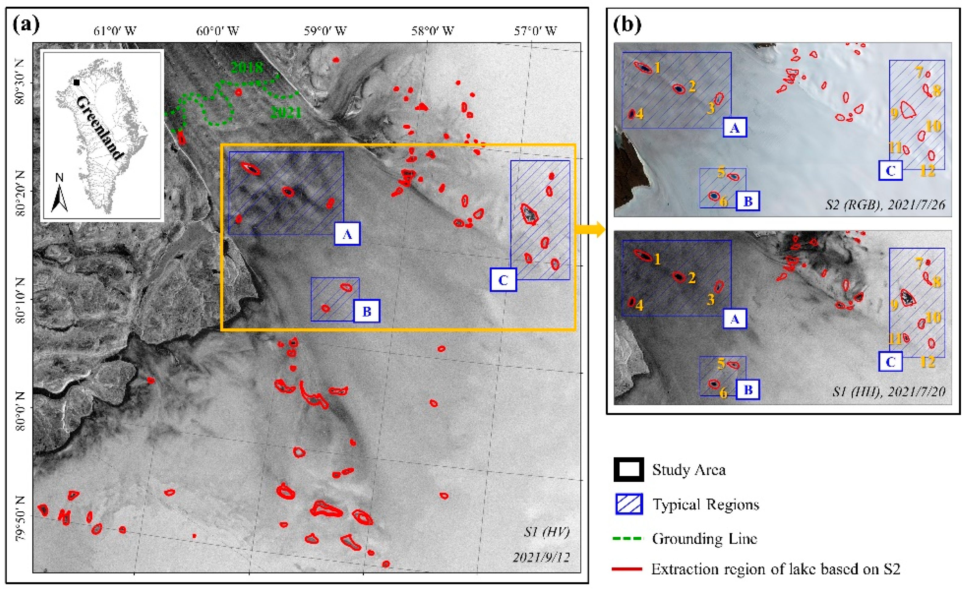
The PG in northern GrIS was chosen as the study area for the experiment (Figure 1). PG is one of the largest outlet glaciers in the north of Greenland, with active surface meltwater [31]. Additionally, this study area contains sufficient optical and SAR satellite images and snow radar passes to favor the validation of the OCO method. Given that one aim of this experiment was to investigate the full-year storage and drainage process, a total of 12 SGLs were included in this study as typical cases (Regions A, B, and C). Fully drained lakes and buried lakes were included in these typical study areas for comparison. As shown in Figure 1b, the lake situation was similar for Regions A and B, which were visible in the optical and SAR images. For Region C, however, the lake could only be observed in the SAR image. Region C was chosen to highlight the importance of SAR imagery in SGL monitoring.
2.2. Satellite Data
The Sentinel series are the Earth observation missions developed by the European Space Agency. In this study, Sentinel-1 and Sentinel-2 were used to extract information of the SGLs. Sentinel-1 and Sentinel-2 images in 2021 were screened for water identification in SAR images, melt/non-melt season imaging comparisons of the SGLs, extraction of monthly changes for the SGLs, and studies of typical drainage phenomena. All Sentinel images were processed in GEE.
The Sentinel-1 mission performs C-band (at a center frequency of 5.405 GHz) SAR imaging, which has some penetration of the shallow snow covering the water [19,32]. Considering image coverage and data quality, the ground range detected (GRD) format with the interferometric wide (IW) swath mode and 10 m pixel spacing from Sentinel-1 SAR images were used in this study. The Sentinel-2 mission comprises a constellation of two polar-orbiting satellites (Sentinel-2A and Sentinel-2B). It is a high-resolution multispectral imaging satellite system carrying a multispectral instrument (MSI) for land surface monitoring. The MSI covers 13 spectral bands and 290 km swath width. For this experiment, we selected Sentinel-2 images with less than 10% cloudiness and applied bands (B2 blue and B4 red) with 10 m spatial resolution for the extraction of SGLs. Sentinel-2 images offer accurate information on supraglacial lake (SGL) extent in favorable weather. Sentinel-1 images, unaffected by weather and lighting, excel in cloud penetration, suitable for diverse environmental observations. Additionally, SAR can penetrate the snow cover, revealing partially buried lakes. Combining Sentinel-1 and Sentinel-2 data not only expands the dataset but also improves SGL localization and year-round monitoring precision.
Snow radar data were used to verify the accuracy and reliability of the extracted lake results that are produced by IceBridge Snow Radar L1B Geolocated Radar Echo Strength Profiles, Version 2 (IRSNO1B) by NASA’s Operation IceBridge (OIB), and radar echograms were taken from the Center for Remote Sensing of Ice Sheets ultrawide-band snow radar over the GrIS. The snow radar operates over the frequency range from ~2 to 6.5 GHz, and it can detect information beneath snow layers to tens of meters in depth [33]. The greater penetration of the snow radar can be used to check the authenticity of SAR-extracted lakes.
3. Methods
3.1. Lake Extraction from Optical Images
Sentinel-2 images used for this experiment were all from GEE’s “COPERNICUS/S2” databases, which contains the Level-1C orthorectified top-of-atmosphere (TOA) reflectance product of the Sentinel-2 satellite, which is widely used for SGL extraction from optical images. In the experiment, the TOA images of Sentinel-2 were pre-processed for the subsequent lake extraction, including date screening, cloud volume filtering (<10%), cloud removal (using the “QA60” band), and clipping. After the pre-treatment, the area with a normalized difference water index adapted for ice () > 0.25 was extracted as the initial extraction area of the lake [34,35].
The blue and red bands in Equation (1) correspond to the reflectance in the blue and red bands for Sentinel-2, respectively. We eliminated SGLs smaller than 5 pixels (30 m resolution) and linear features narrower than 2 pixels, which have relatively large uncertainties, to improve the extraction accuracy for SGLs further [15,36]. Considering the possible influence of clouds in the images and the irrelevant location migration of the SGLs on the ice sheet surface, we superimposed all the lake areas extracted by > 0.25 for the melt season (from May to September) during the study period and selected the area with more than five recurrence times as the area with the largest water mask.
3.2. Otsu–Canny–Otsu Method for SGL Extraction
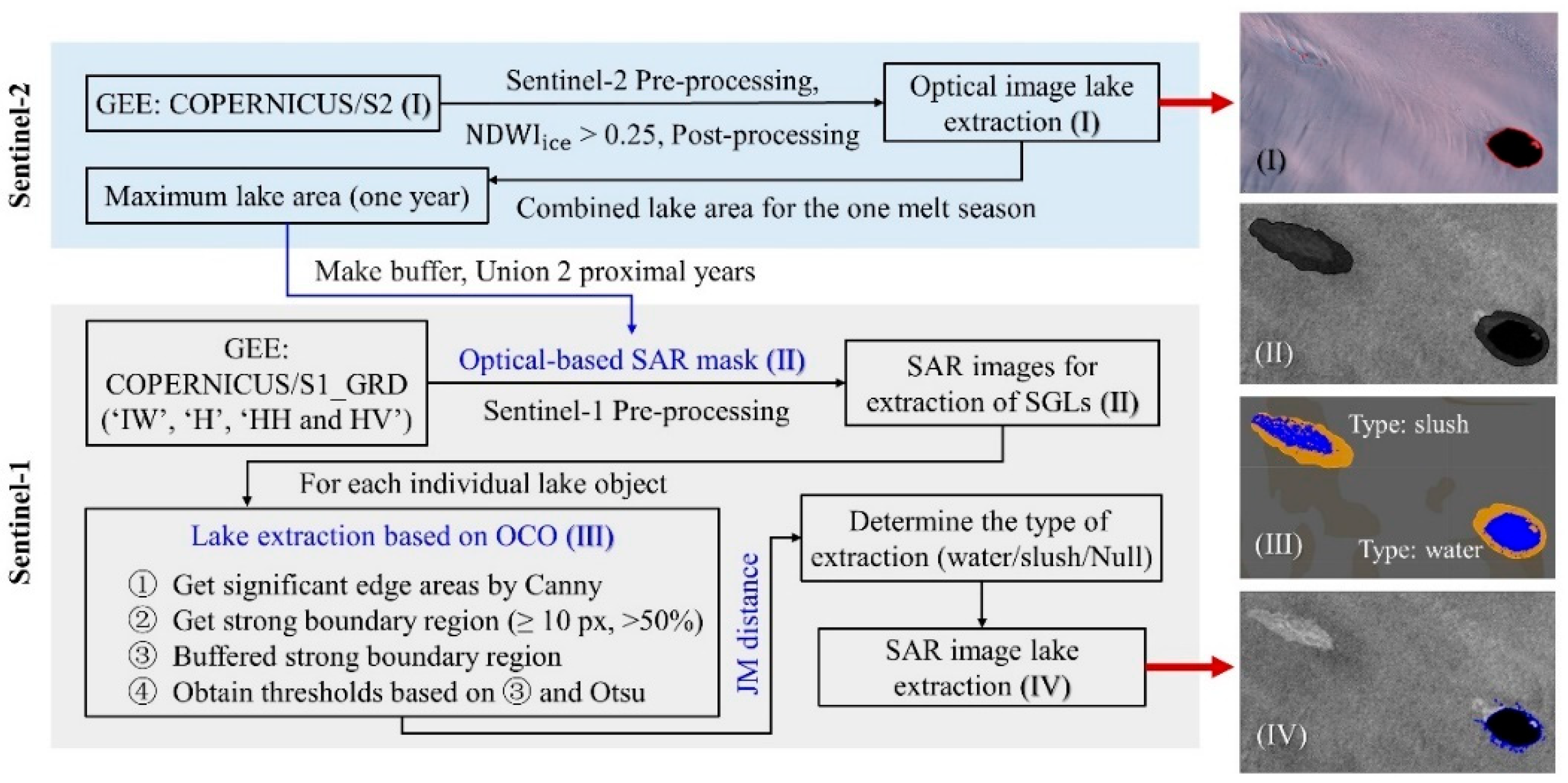
Extraction using the OCO model is divided into the following five steps: Sentinel-1 data acquisition, Sentinel-1 data pre-processing, mask fabrication for SAR extraction area based on the optical image, lake extraction in SAR based on the OCO method, and postprocessing for the lake area (Figure 2).
- (1)
- Sentinel-1 data acquisition: Sentinel-1 images were selected from GEE’s “COPERNICUS/S1_GRD” product. The parameter “instrumentMode” is “IW”, which contains HH and HV polarization. Image quality is “H” with a resolution of 10 × 10 m. The GRD product in GEE already contains most of the pre-processing steps (thermal noise removals, data calibration, multilooking, and range-Doppler terrain correction) of Sentinel-1 [37].
- (2)
- Sentinel-1 data pre-processing: The topographic correction of the study area was conducted using the Greenland Mapping Project, a Greenland digital elevation model (DEM) product that comes with the GEE platform (https://developers.google.com/earth-engine/datasets/catalog/OSU_GIMP_DEM) (accessed on 6 November 2023), which enables the SAR images to have better feature recognition in areas with large topographic relief. To minimize the influence of the original noise of SAR images on feature extraction, the Lee sigma filter was applied to the images [37,38].
- (3)
- Mask fabrication of the SAR extraction area based on optical image: The lake exhibits low backscatter intensity in the SAR image, appearing nearly black [39]. However, many non-water regions in SAR also exhibit low backscatter intensity due to topographic features. To pinpoint the area where the SGL appears in SAR images, we utilized the combined maximum lake area from two consecutive melt seasons (May to September each year) in the optical image as the SAR extraction area [18,19].
This experiment adopted the concept of maximum lake area, which is the maximum area covered by the lake extracted in the optical image during one melt season. The possible lake extent between two melt seasons can be obtained by superimposing the maximum lake area for the two proximal years. Before making the masking area for SAR extraction, applying a buffer for maximum lake area was necessary due to slush surrounding some lakes having similar backscatter values to the lakes, thereby complicating the differentiation of slush and water [18]. The size of the radius of the buffer zone is determined by the size of the individual lakes. The final SAR masking area is obtained by superimposing the two-buffering maximum lake area of the proximal years. The maximum lake areas for 2020, 2021, and 2022 were used in this experiment.
- (4)
- Lake extraction in SAR based on the OCO method: The SGLs were extracted from Sentinel-1 with HH and HV polarization. HH polarization was used for lake extraction of SAR during the melt season, and HV polarization was used to extract the lake that was covered by snow during the non-melt season [40]. The experiment first clipped the pre-processed image of the SAR using the masked area of the SAR in (3) and calculated the input value of the Canny algorithm using OTSU for a single lake area, resulting in remarkable edge areas in the SAR image. The edge areas must be bordered in GEE. Second, fragmented remarkable edges of less than 10 pixels were removed, and the top 50% of the edge strength was selected as the strong boundary region. Third, a two-pixel buffer was made outward of the strong boundary region, which contained the two most varied classes in SAR images of a single lake mask. Finally, the buffered strong masked regions were used as the basis for the extraction of Otsu thresholds to obtain classification thresholds for the two classifications in SAR images. This threshold was used to separate the remarkable regions in the SAR image [18].
- (5)
- Post-processing for lake area: After acquiring areas that differ considerably from the surrounding environment, whether the extracted area contains water (low backscattering coefficient) or slush (high backscattering coefficient) must be determined. Three regions of a single lake were selected for comparison in the experiment. The analyzed regions were the high backscatter region of the extracted region (classes g), the low backscatter region of the extracted region (classes l), and the backscattering intensity of the 30 pixels expanded around the extracted region (classes a). The experiment used the Jeffries–Matusita distance (JM distances) to discuss the differences between the three regions and to distinguish between areas of open water and slush, as well as partially misdivided areas without water (Equations (2) and (3)). The JM distance is an indicator of difference degree between classes. It ranges from 0 to 2, and the larger it is, the more considerable the difference between classes [41]. In our experimental statistics, we considered that a discernible difference existed between the classes when JM > 1 for the two types of features [42].
indicates the JM distance between two classes; g, l, and a indicate the three classes for distinction. They are the high backscatter region of the extracted region, the low backscatter region of the extracted region, and the backscattering intensity of the 30 pixels expanded around the extracted region, respectively. The primary objective of this approach is to assess if there is a real feature in the area obtained based on the OCO method, and if this feature is a lake. After determining the presence of lakes, areas smaller than 20 pixels were removed to reduce the effect of SAR noise, and the small hole in the water was clumped. The final processed data were the area of the SGLs extracted based on SAR images.
4. Results
4.1. Lake Detection
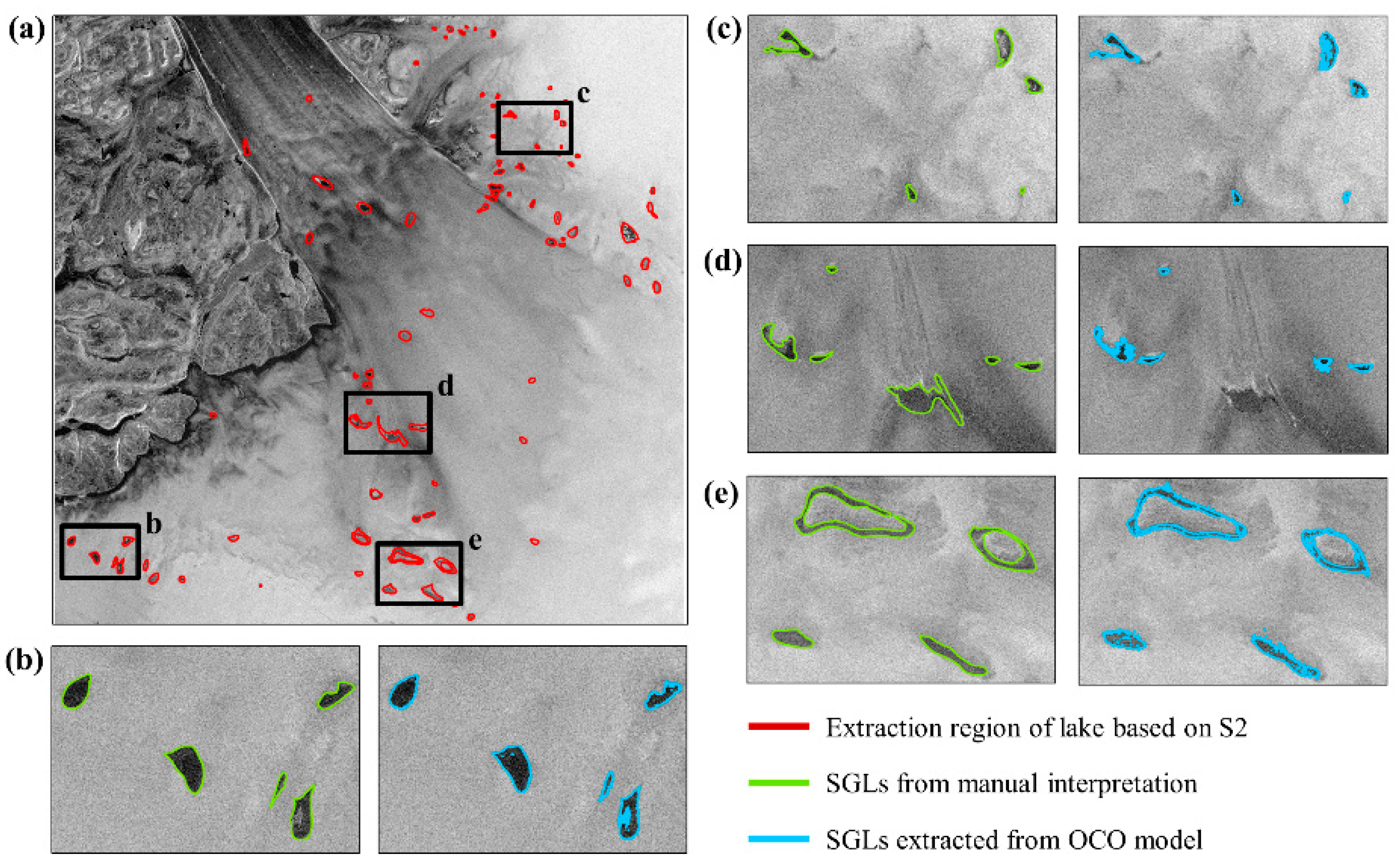
It is challenging to evaluate the performance of the OCO method due to the absence of ground truth. Here, we compared the OCO extraction results with the manual extraction results with the HH-polarized SAR image of 12 September 2021 in the study area (Figure 3). As shown in the four examples in Figure 3, the lake extracted from the SAR image by the OCO method matched the results of the manual interpretation. The lake acquired by the OCO method contained more scattered pixels—some of them were noise from the SAR imagery, and some of them were details of water that were not refined by the visual interpretation. There were also omissions in the OCO-extracted results, e.g., the obvious SGL in the middle of Figure 3d was not extracted with the OCO method.
Our study included 85 lake mask areas, and only two lake objects were not decoded by the OCO method from the 72 lakes that existed in the visual interpretation of this SAR image. In order to verify the accuracy of the OCO model, a confusion matrix based on the OCO extraction results and the manual extraction results was computed, and the calculated pixel range was the maximum lake area. By calculating the true positive (TP), false negative (FN), false positive (FP), and true negative (TN) rates in the confusion matrix, the performance of the algorithm could be measured as follows: overall accuracy was 0.885, precision was 0.929, recall was 0.749, the F1 score was 0.829, and the Kappa coefficient was 0.745.
To compare the differences in lake extraction between optical and SAR images in the melt season, we extracted 12 typical SGLs from optical and SAR images of the study area on 26 July 2021, respectively, with the SAR image using HH polarization. Lake 6 results were supplemented with the 24 July SAR image as the 26 July SAR image could not cover all 12 lake objects. Table 1 shows the SGL extraction results of the optical image using , the SGL extraction results of the SAR image based on the OCO method, and the SGL area of visual interpretation based on SAR images. For the 12 SGLs on 26 July 2021 (supplemented on 24 July), six SGLs were extracted from the optical image, appearing in Regions A and B; 12 SGLs were obtained in SAR-based manual extraction; and 11 SGLs were obtained in the SAR-based OCO method, for which Lake 3 was not extracted. Comparing the SGL extraction results of optical and SAR images showed that optical and SAR images could extract the lakes in Regions A and B, but only the SAR image could extract the lake in Region C, which was completely covered by snow. The water extraction area of the optical image was generally larger than that of the SAR image, with a difference basically below 0.3 km2. Region B showed a greater difference between optical and SAR water extraction areas than Region A did. Except for Lakes 7 and 12 that had a larger difference, the difference between the lake area acquired from the automatic OCO method and the manually mapped one was around 20%.
Lake 3 was not successfully extracted when determining the existence of a lake in SAR images based on the JM distance. The JM distance between the backscattering intensity around the lake and inside the lake for Lake 3 was small, i.e., only 0.676, which did not satisfy the judgment that JM distance > 1. The other 11 lakes’ JM distances were all in the range of 1.3 to 1.9, with good separation.
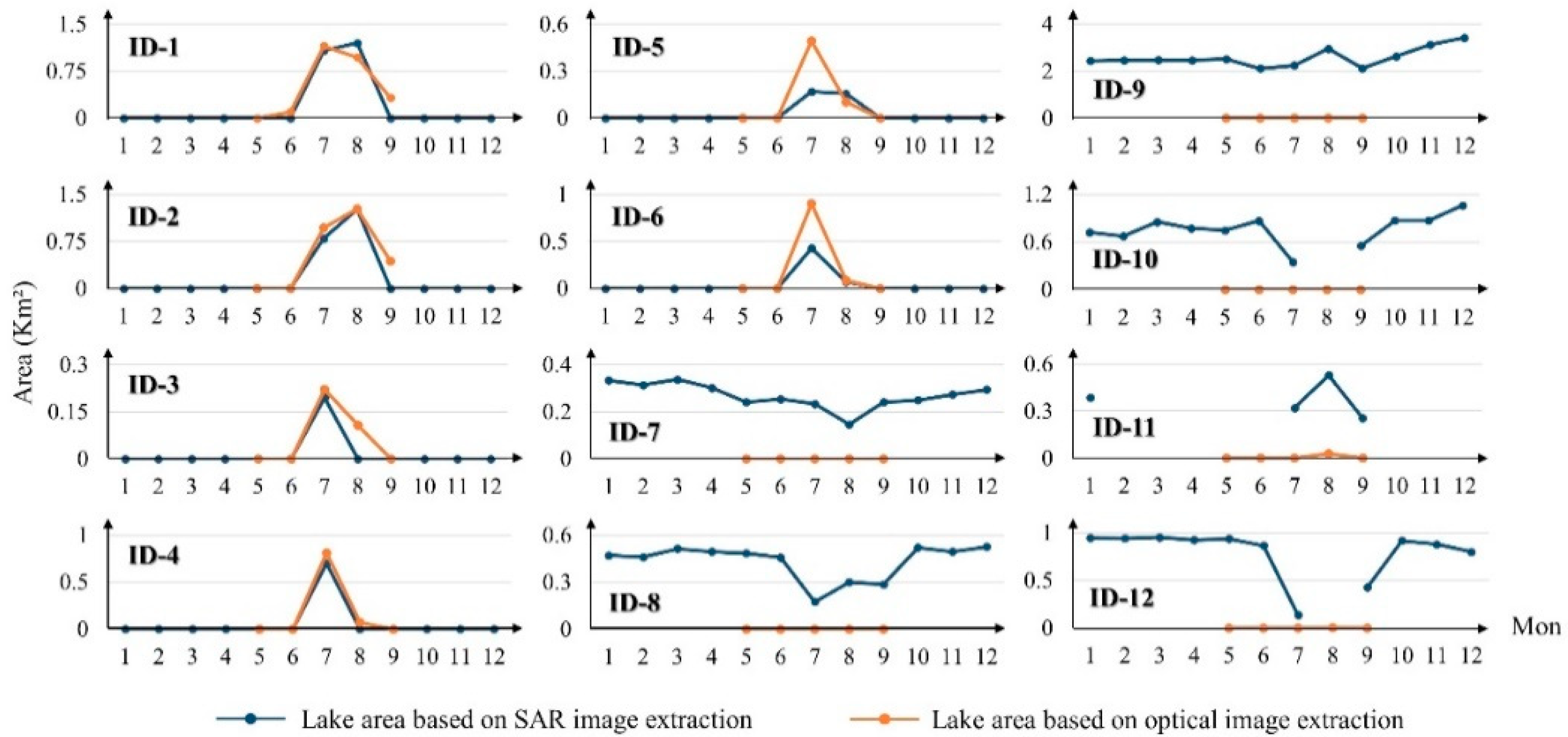
4.2. Full-Year SGLs Changes in 2021
The experiment monitored and extracted monthly SGL data from January to December in 2021. The results included optical and SAR-extracted data for 12 typical lakes, which were divided into three regions (Regions A, B, and C) for separate discussions (Figure 4). For SAR images, the data for May, June, July, August, and September were in HH polarization; and October, November, December, the following year’s January, February, March, and April were in HV polarization.
The SGL changes were similar in Regions A and B. The lakes in these areas developed and drained during the melt season, with the peak occurring in July and August. The development of the SGL was well monitored by optical and SAR imagery during the melt season, with the same trends in the two types of imagery. The SAR and optical extraction results were slightly different, with the area extracted from SAR being smaller than that extracted from the optical images.
Large differences were observed between Region C and Regions A and B. The optical images only detected the area of three SGLs (Lake 10, 11, and 12) in August. However, the extraction of the SAR images showed that all six lakes in Region C were already present in January 2021, and only a slight change in area occurred from January to June for those lakes. For Region C, SAR imagery was slightly effective in detecting images during the melt season, especially in August when water was difficult to detect completely. The SGLs were still detectable in SAR imagery in September, October, November, and December after the melt season. The change in lake area after the melt season from the pre-melt season was small, with less than 25%. In particular, the area of Lakes 8 and 12 changed by less than 10% before and after the melt season. The experiments also compared the results from May to September in Region C for HH and HV polarization, and the area difference between the two polarizations was in the range of 15–20%, with no remarkable improvement in the extracted lakes.
4.3. Lake Drainage Monitoring
To discuss the time series changes of the lake at a finer scale, Lakes ID-4 and ID-5 were selected for the experiment to explore the changes in storage and discharge from 1 July to 31 August 2021. The experiment combined SAR and optical data. Fewer optical images were available, with only July 26 available in July and seven date images available in August. SAR imagery was denser than the optical imagery over the area of the studied SGLs, with 10 and 11 images for July and August, respectively.
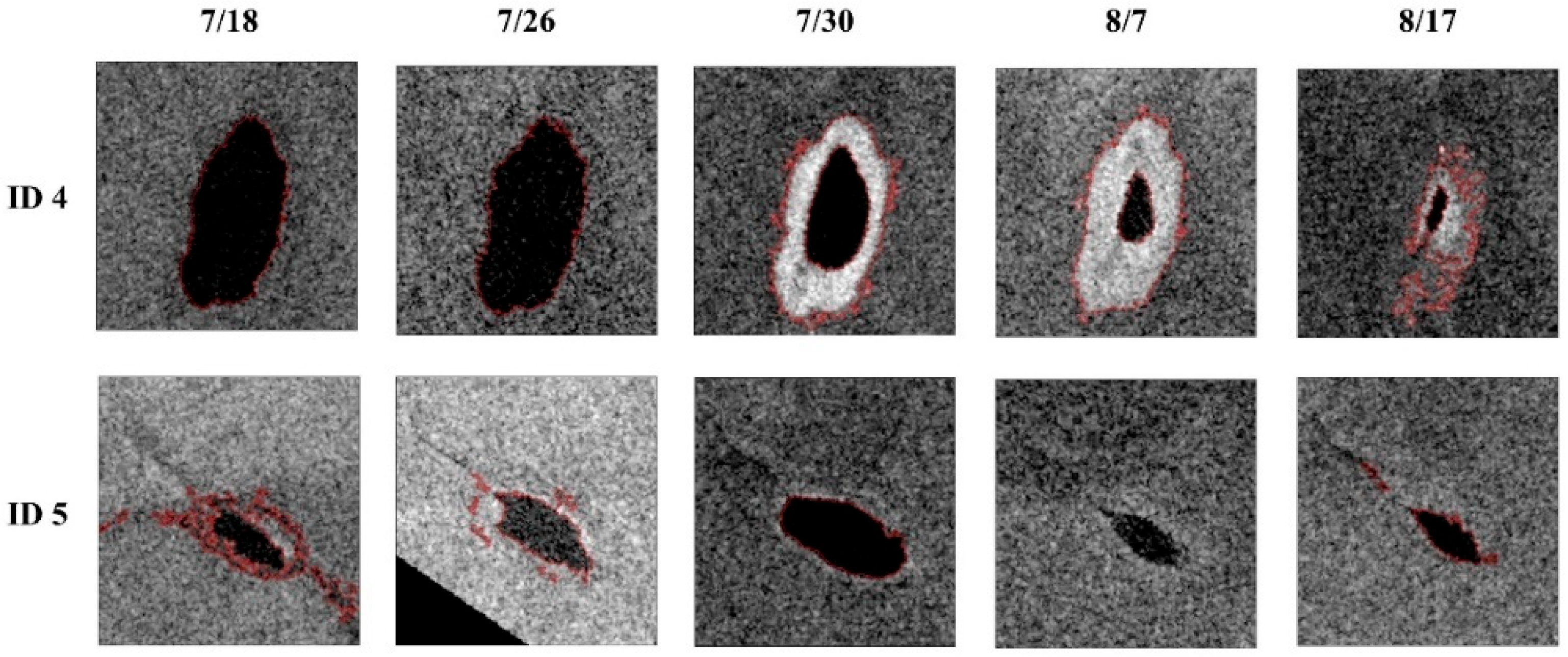
Figure 5 excerpts the Sentinel-1 HH polarization images of Lakes ID-4 and ID-5 at several typical time points during the storage and drainage period. Lake ID-4 experienced a dramatic drainage event from 26 to 30 July, accompanied by the production of slush around the lake. The change in area of Lake ID-5 was more moderate, with drainage occurring from 30 July to 7 August. Lake ID-5 was scattered in extent at the beginning of the melting, with the water gradually pooling into a whole lake during the storage process.
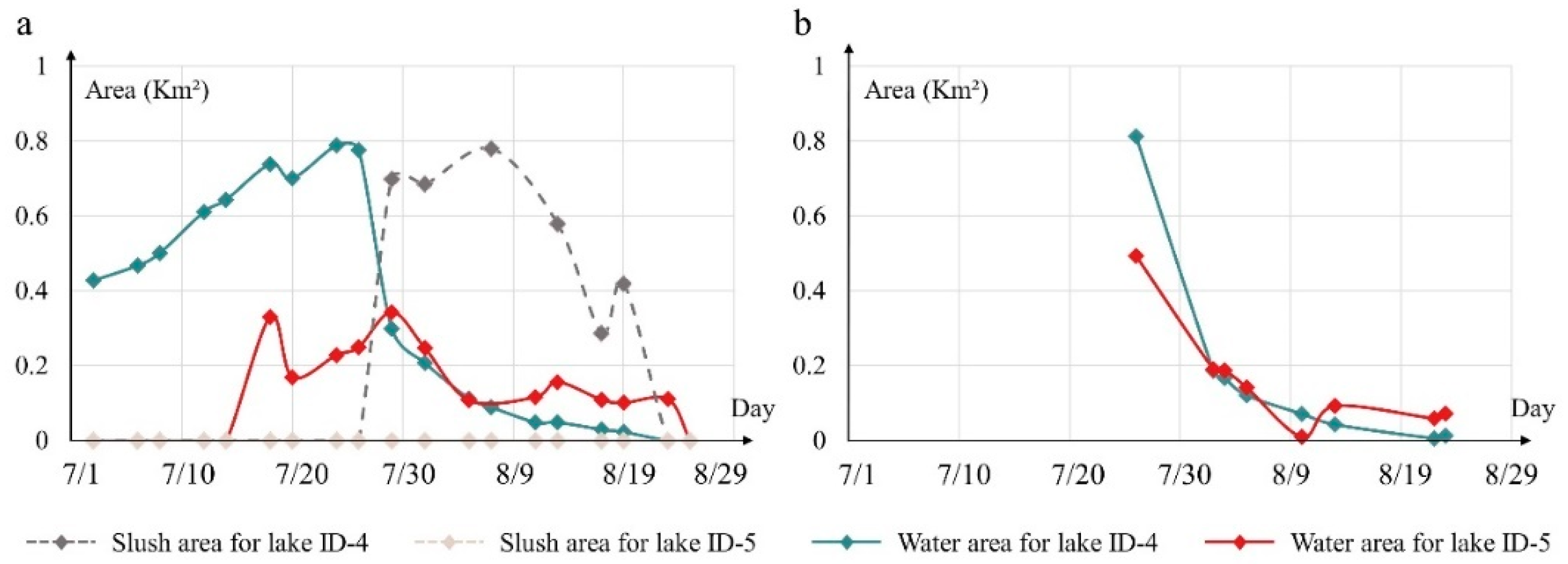
The changes of water area occurring in July and August 2021 for two typical SGLs, ID-4 and ID-5, are shown in Figure 6. Lake ID-5 began to accumulate water on July 18, reaching the maximum area of water detected by SAR on 18 and 30 July, and the water completely disappeared on 25 August. Between 30 July and 5 August, the lake underwent a relatively strong drainage event, with the water area dropping from 0.343 km2 to 0.108 km2. The area of Lake ID-5 remained around 0.1 km2 after 5 August until water could not be extracted in the SAR in 23 August. At the beginning of the melt, on 18 July, Lake ID-5 was monitored in SAR to a larger area of 0.345 km2. During this period, the SGL was in the early stages of catchment, and some shallow meltwater was found, all of which was included in the SAR imagery as water areas.
Drainage was more pronounced at Lake ID-4 than at ID-5. The results of the area change showed that Lake ID-4 was drained from 26 to 30 July, with the area dropping from 0.776 km2 to 0.300 km2, a 61.3% reduction in area over the four days. Extensive slush formed from the drainage of the SGL could be clearly detected in the SAR image on 30 July (Figure 6a). After 30 July, the area of the SGL continued to decline and completely disappeared on August 23. During the drainage period, the area of slush also changed. From 30 July to 7 August, the slush area tended to increase, reaching a maximum area of around 0.7 km2. After 7 August, the slush area decreased considerably until it disappeared.
5. Discussion
5.1. Advantages of Multisource Remote Sensing
Optical and SAR imagery could be effectively used to extract information about SGLs. However, given the characteristics of optical and SAR imaging, flaws and differences were found in the extraction results between the two types. The area extracted from -based optical images of the lake was simple and straightforward, but the quality of some images was poor because of the weather and snow cover, resulting in fewer data sources being available for SGL extraction. SAR satellites have better penetration and are effective in avoiding cloud effects on images and detecting thin snow-covered lakes. C-band SAR images are generally not hindered by atmospheric effects and are capable of imaging through tropical clouds and rain showers. Its penetration capability with snow on the ground is limited, usually around 1 to 2 m [43], and the specific depth of snow penetration is related to the physical properties of the snow and the radar’s incidence angle [44].
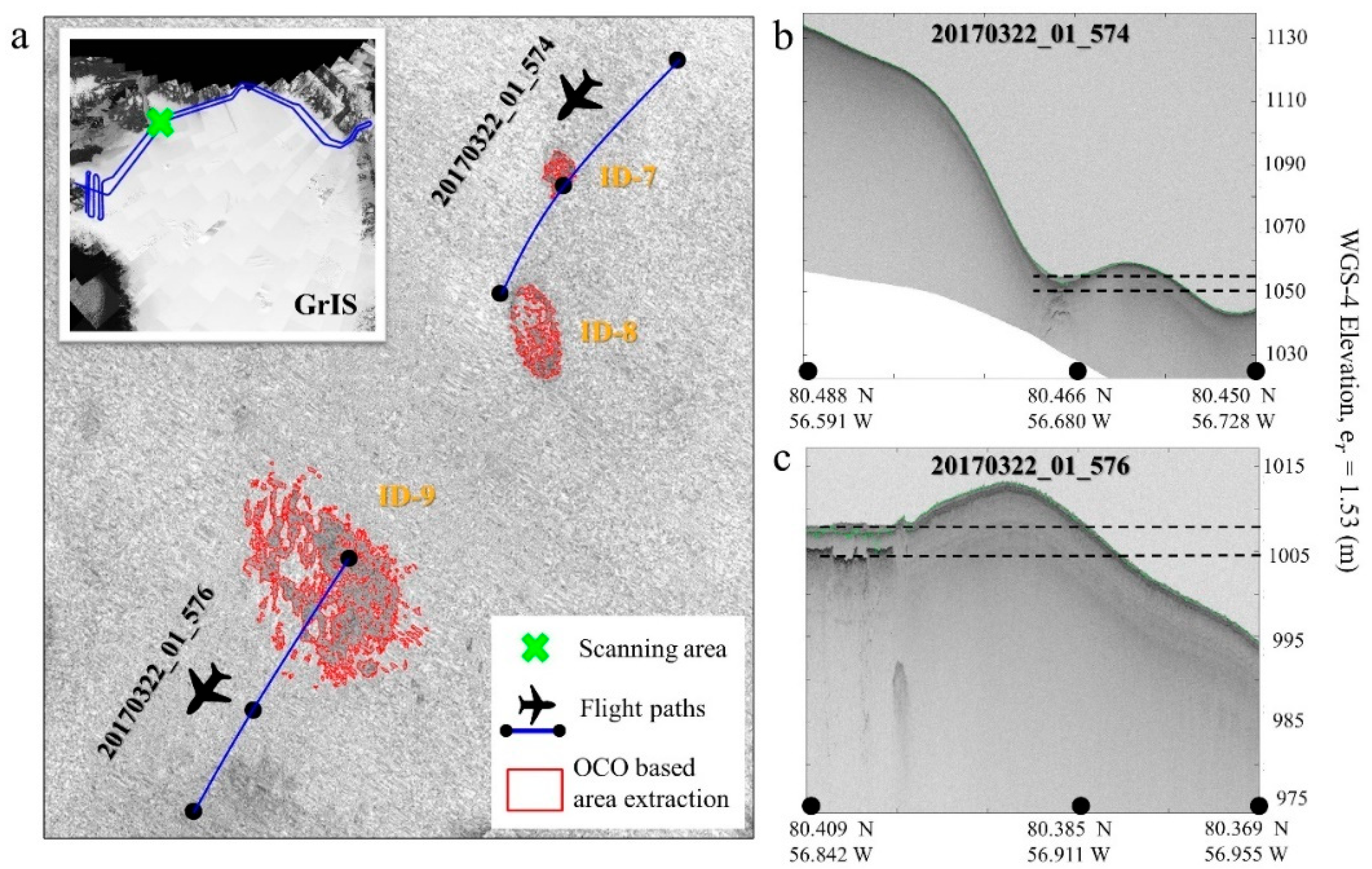
Optical images can only identify exposed lakes on the ice sheet and cannot detect the lake covered by ice floes and thin snow. This kind of buried lake is widespread in the GrIS at all times of the year in melt and non-melt seasons. SAR imagery can detect buried lakes covered by shallow snow partially, but lakes buried under a thicker ice cover are difficult to detect from SAR imagery. For monitoring validation of buried lakes, snow radar data collected by NASA’s OIB were chosen. Snow radar data have greater penetration and can be used to estimate the cross section of glaciers. Figure 7a shows the echogram results obtained by a snow radar on 22 March 2017, when lakes had no optical visibility. Comparing Sentinel-1 results from 23 March of the same year showed that Sentinel-1 could detect well the water located under the ice surface. The monitored water was covered with snow at a thickness of about 3 m (Figure 7b,c). The comparison showed that the SAR-based approach to lake extraction expanded the data for buried lakes, thus providing additional data support for a comprehensive analysis of the seasonal variability of SGLs.
This study used Sentinel-1 and Sentinel-2 images to monitor SGL transformations during the melt and non-melt seasons. The experimental method combined the characteristics of SAR imagery with optical imagery, addressing the limitations of optical images in winter and the greater environmental noise of SAR images in part. Additionally, it is important to note that due to the limited penetration capability of C-band SAR imagery, there may be more buried lakes in areas where C-band SAR signals cannot reach [45].
5.2. Factors Affecting Water Extraction in SAR
HH and HV polarization are two common types of polarization used in SAR imagery, and the choice of polarization can affect the effectiveness of lake extraction [46,47]. HV polarization often shows a better contrast between water and snow in areas of buried water. The reason for this situation is that HH polarization is more susceptible to the radar signal with the top snow layers, resulting in less information acquired in HH polarization than in HV polarization for buried lakes [32]. For open water, the backscattering in HH polarization is more stable than in HV backscattering [48]. Hence, HH polarization can distinguish open-water and high-water content snow in more cases than HV polarization can.
SAR imagery has the advantage of being available in all weather and being able to penetrate thin snow; however, it is susceptible to external factors, such as the angle of incidence, the melting state of the ice surface, wind, etc., when detecting SGLs on the ice sheet [18,49,50]. These external influences can lead to variations in the backscatter intensity of the SAR image, resulting in the inability to extract lakes from a SAR image. Many anomalies in the extraction of SGLs from SAR imagery occurred in this experiment. For example, during lake extraction of month-by-month SAR imagery for 2021, the SAR image in August of Region C was poorly imaged, with the entire zone exhibiting lower backscatter intensity (Figure 4). During drainage monitoring of Lakes ID-4 and ID-5 in late July and early August, no information was obtained for Lake ID-5 in the 7 August SAR image (Figure 5). Furthermore, in lake detection of Section 4.1, Lake ID-3 was not identified due to the poor separation () of the lake and surrounding area backscatter intensities (Table 1). In summary, the most important reason for not being able to extract water from SAR images is that water has a backscatter intensity similar to that of the surrounding environment, making it difficult to distinguish water from the environment in SAR images.
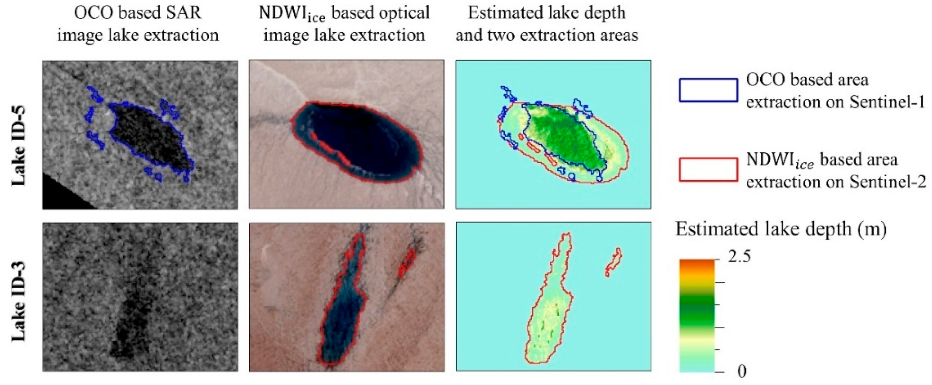
Some differences were also found between the optical results and the SAR results in lake extraction at nearly the same time. We compared the SGLs in Regions A and B, which could be extracted from the optical image (imaging time 18:10 UTM) and SAR (imaging time 11:36 UTM) in the study area on 26 July 2021 (Figure 8), and the results showed that the difference was mainly in Lake ID-5, with a 2.30-fold difference in extraction between the two types of images. We calculated the water depth distribution of Lake ID-5 using the water depth formula for optical imagery [12,51] and found that the main difference in water extraction area between optical and SAR imagery came from shallow water areas, mainly below <0.75 m. A similar situation occurred for Lake ID-3, which was not identified in the SAR image. The SAR lake extraction area of some of the lakes was also found to be slightly smaller than the optical lake extraction area in Section 4.3 (Figure 4). On the basis of these results, we inferred that the depth of the open lake would influence the imaging results of the water area in the SAR [18]. The temporal difference between Sentinel-1 and Sentinel-2 images in this test could also be the cause of this error.
SGL extraction in SAR is influenced by external natural factors and the lake’s own properties, which may lead to some challenges in accurate SAR-based lake area extraction for time series.
5.3. Drainage Monitoring
Optical image-based SGLs drainage has been widely used in SGL change detection [52]. In Section 4.3, we monitored the drainage process of two lakes, i.e., Lakes ID-4 and ID-5, from July to August 2021. Lakes ID-4 and ID-5 had two types of drainage processes, fast and slow, respectively (Figure 5 and Figure 6). Although rapid drainage of SGLs could also be detected using the optical images in the experiment (Figure 6b), the limited amount of available optical images did not allow for a better reproduction of SGL development. Rapid drainage of SGLs in SAR is often accompanied by a sudden increase in the intensity of backscatter around the lake (Figure 5). The reason for this phenomenon is that rapid drainage leaves behind some rough heterogeneous surface consisting of patches of slush and ice, producing high backscatter values. Over time, these slush and ice blocks smooth out, and the backscatter values match those of the surrounding environment. Thus, rapid drainage can also be monitored by high backscatter from lake anomalies, but this is not always featured in the imagery [18].
During optical and SAR image monitoring of the SGLs in Region C in 2021, the SGLs were barely visible in the optical images of Region C, with only a small area showing during the peak melt season (Figure 4). However, the detection of SGLs in SAR imagery revealed that the lake was always present in Region C and that some of the lakes did not change considerably in area before and after the melt season (Figure 4). The change of area of the lake in Region C was less than 25% before and after the melt season and even less than 10% in Lakes 8 and 12 due to the presence of buried lakes. Some lakes do not drain nor freeze completely as they enter winter; they are stored as liquid water under the frozen snow and ice layers, forming a buried lake [53]. Therefore, it is ambiguous to judge SGL drain by the area change in the optical image. It may underestimate the actual area of water stored on the ice sheet and overestimate the drainage of SGLs at the end of the melt season.
5.4. Limitations and Prospects
SGL extraction results in SAR images based on the OCO method in the experiment are always dichotomous; however, the boundary between the backscattering intensities of water and non-water in a region is challenging to characterize with a single threshold. At the same time, the availability of SAR imagery is not completely established and is affected by factors, which can also affect the results of the time-dependent detection of SGLs. Therefore, we will analyze how to maximize SAR images and reduce the noise associated with threshold extraction methods in following research. The main purpose of this experiment was to verify the feasibility of the OCO method and the importance of SAR imagery in SGL monitoring. In future studies, the study area will be expanded, and SGL changes across the cryosphere will be discussed by fusing the time series of multisource remote sensing data.
6. Conclusions
SGL changes are an important monitoring object of ice sheets that reflects the volume change of ice sheet surface melting. With the development of remote sensing technology, the monitoring of SGL changes based on remote sensing observation has been gradually improved. Optical and SAR remote sensing has been widely used in the detection of SGLs. However, given the vulnerability of optical imagery to the weather, the amount of optical data that can be practically applied is limited. Meanwhile, information on buried lakes is not available in winter from optical imagery. Although SAR has good penetration and a large volume of data, it presents a backscattered intensity signal with a dense “homospectral foreign object” situation over a large area. Effective extraction of SGL information from optical and SAR imagery allows improved monitoring of SGL development throughout the year.
This study proposed a new model named the OCO method. It combines optical and SAR satellites and the Otsu algorithm and Canny edge detector to investigate the development of SGLs throughout the year. Optical images can locate SGLs more accurately, and SAR images have a degree of penetration of clouds and snow. Based on optical and SAR data, the changes in the SGLs can be better monitored throughout the year. In terms of extraction methods, is used to extract the lake area from the optical images, and the OCO method is used to extract the SGLs’ area from the SAR images masked by the maximum lake area of optical images. The OCO method performs feature extraction for each individual SGL based on the Otsu–Canny edge detection algorithm and the Canny edge Otsu algorithm, and it is built to be more objective and targeted.
The experiment validated the accuracy of the OCO method for SGLs extraction, together with monitoring the full-year variations of typical lakes based on Sentinel-1 and Sentinel-2 images in 2021. Benchmarked against the manual SGLs extraction result, the OCO method performed well overall accuracy of 0.885 and F1 score of 0.829. In the OCO method for SGL extraction, SAR images can be affected by external natural factors, such as incidence, surface melting, wind, and other factors, resulting in the inability to extract SGLs properly. The difference between the SAR results of extracting SGLs based on the OCO method and the visual interpretation was around 20%. During the same period, the depth of the lake may influence the extraction range of SGLs in different types of imagery. Experimental results indicated that shallow lakes were challenging to observe in SAR images (<0.75 m in this experiment). SAR imagery had higher data density in the study area than optical imagery did and could monitor SGL development during the non-melt season, which was the result that could not be acquired with optical imagery. For the 12 typical SGLs in the study area in 2021, some of the lakes were stored and drained during the melt season (Region A and B), but some SGLs did not change considerably before and after the melt season (Region C). The SGLs in Region C, although no longer detectable on optical imagery during the non-melt season, were consistently detectable in SAR imagery with 10–25% changes in area. Validation of the snow radar data revealed the presence of buried lakes under ice in this area. As SAR imagery had more intensive data in the study area than optical imagery did, this experiment also detected a rapid drainage event of the SGLs over a four-day period.
Combining optical and SAR imagery for monitoring changes allows for better discussion of the annual and seasonal variation of SGLs, allowing for analysis of hydrological events with more intensive time series. The OCO method proposed in this study can combine the advantages of optical and SAR imagery and consider the buried lakes during winter storage of water. This approach avoids the overestimation of the discharge of the SGLs after the melt season that would result from monitoring the lake using optical images only.
Author Contributions
Conceptualization, D.Z. and C.Z. (Chunxia Zhou); Methodology, D.Z., C.Z. (Chunxia Zhou) and C.Z. (Ce Zhang); Software, Y.Z.; Validation, Y.Z.; Investigation, Y.Z. and T.W.; Resources, C.Z. (Ce Zhang); Data curation, T.W.; Writing—original draft, D.Z.; Writing—review & editing, C.Z. (Chunxia Zhou), Y.Z. and C.Z. (Ce Zhang); Supervision, C.Z. (Ce Zhang); Funding acquisition, C.Z. (Chunxia Zhou) and C.Z. (Ce Zhang). All authors have read and agreed to the published version of the manuscript.
Funding
This work was supported by the Natural Environment Research Council (grant number NE/T004002/1) and was partially funded by the National Key Research and Development Program of China (2021YFC2803303) and the National Natural Science Foundation of China (NSFC) (42171133, 41776200).
Data Availability Statement
Data available on request due to restrictions privacy. The data presented in this study are available on request from the first author.
Conflicts of Interest
The authors declare no conflict of interest.
References
- Van Wychen, W.; Hallé, D.A.M.; Copland, L.; Gray, L. Anomalous Surface Elevation, Velocity, and Area Changes of Split Lake Glacier, Western Prince of Wales Icefield, Canadian High Arctic. Arct. Sci. 2022, 8, 1288–1304. [Google Scholar] [CrossRef]
- Van Wychen, W.; Bayer, C.; Copland, L.; Brummell, E.; Dow, C. Radarsat Constellation Mission Derived Winter Glacier Velocities for the St. Elias Icefield, Yukon/Alaska: 2022 and 2023. Can. J. Remote Sens. 2023, 49, 2264395. [Google Scholar] [CrossRef]
- Hogg, A.E.; Shepherd, A.; Gourmelen, N.; Engdahl, M. Grounding Line Migration from 1992 to 2011 on Petermann Glacier, North-West Greenland. J. Glaciol. 2016, 62, 1104–1114. [Google Scholar] [CrossRef]
- Zhu, Y.; Zhou, C.; Zhu, D.; Wang, T.; Zhang, T. Interannual Variation of Landfast Ice Using Ascending and Descending Sentinel-1 Images from 2019 to 2021: A Case Study of Cambridge Bay. Remote Sens. 2023, 15, 1296. [Google Scholar] [CrossRef]
- Pattyn, F.; Ritz, C.; Hanna, E.; Asay-Davis, X.; DeConto, R.; Durand, G.; Favier, L.; Fettweis, X.; Goelzer, H.; Golledge, N.R.; et al. The Greenland and Antarctic Ice Sheets under 1.5 °C Global Warming. Nat. Clim. Chang. 2018, 8, 1053–1061. [Google Scholar] [CrossRef]
- Mouginot, J.; Rignot, E.; Bjørk, A.A.; van den Broeke, M.; Millan, R.; Morlighem, M.; Noël, B.; Scheuchl, B.; Wood, M. Forty-Six Years of Greenland Ice Sheet Mass Balance from 1972 to 2018. Proc. Natl. Acad. Sci. USA 2019, 116, 9239–9244. [Google Scholar] [CrossRef]
- Slater, T.; Shepherd, A.; McMillan, M.; Leeson, A.; Gilbert, L.; Muir, A.; Munneke, P.K.; Noël, B.; Fettweis, X.; van den Broeke, M.; et al. Increased Variability in Greenland Ice Sheet Runoff from Satellite Observations. Nat. Commun. 2021, 12, 1–9. [Google Scholar] [CrossRef]
- Hoffman, M.J.; Perego, M.; Andrews, L.C.; Price, S.F.; Neumann, T.A.; Johnson, J.V.; Catania, G.; Lüthi, M.P. Widespread Moulin Formation During Supraglacial Lake Drainages in Greenland. Geophys. Res. Lett. 2018, 45, 778–788. [Google Scholar] [CrossRef]
- Abdalati, W.; Steffen, K. Passive Microwave-derived Snow Melt Regions on the Greenland Ice Sheet. Geophys. Res. Lett. 1995, 22, 787–790. [Google Scholar] [CrossRef]
- Leeson, A.A.; Shepherd, A.; Briggs, K.; Howat, I.; Fettweis, X.; Morlighem, M.; Rignot, E. Supraglacial Lakes on the Greenland Ice Sheet Advance Inland under Warming Climate. Nat. Clim. Chang. 2015, 5, 51–55. [Google Scholar] [CrossRef]
- Zhu, D.; Zhou, C.; Zhu, Y.; Peng, B. Evolution of Supraglacial Lakes on Sermeq Avannarleq Glacier, Greenland Using Google Earth Engine. J. Hydrol. Reg. Stud. 2022, 44, 101246. [Google Scholar] [CrossRef]
- Banwell, A.F.; Willis, I.C.; Macdonald, G.J.; Goodsell, B.; MacAyeal, D.R. Direct Measurements of Ice-Shelf Flexure Caused by Surface Meltwater Ponding and Drainage. Nat. Commun. 2019, 10, 730. [Google Scholar] [CrossRef] [PubMed]
- Banwell, A.F.; MacAyeal, D.R.; Sergienko, O.V. Breakup of the Larsen B Ice Shelf Triggered by Chain Reaction Drainage of Supraglacial Lakes. Geophys. Res. Lett. 2013, 40, 5872–5876. [Google Scholar] [CrossRef]
- Lemos, A.; Shepherd, A.; McMillan, M.; Hogg, A.E. Seasonal Variations in the Flow of Land-Terminating Glaciers in Central-West Greenland Using Sentinel-1 Imagery. Remote Sens. 2018, 10, 1878. [Google Scholar] [CrossRef]
- Williamson, A.G.; Banwell, A.F.; Willis, I.C.; Arnold, N.S. Dual-Satellite (Sentinel-2 and Landsat 8) Remote Sensing of Supraglacial Lakes in Greenland. Cryosphere 2018, 12, 3045–3065. [Google Scholar] [CrossRef]
- Dunmire, D.; Banwell, A.F.; Wever, N.; Lenaerts, J.T.M.; Datta, R.T. Contrasting Regional Variability of Buried Meltwater Extent over 2 Years across the Greenland Ice Sheet. Cryosphere 2021, 15, 2983–3005. [Google Scholar] [CrossRef]
- Ghiasi, Y.; Duguay, C.R.; Murfitt, J.; Asgarimehr, M.; Wu, Y. Potential of GNSS-R for the Monitoring of Lake Ice Phenology. IEEE J. Sel. Top. Appl. Earth Obs. Remote Sens. 2023, 17, 660–673. [Google Scholar] [CrossRef]
- Miles, K.E.; Willis, I.C.; Benedek, C.L.; Williamson, A.G.; Tedesco, M. Toward Monitoring Surface and Subsurface Lakes on the Greenland Ice Sheet Using Sentinel-1 SAR and Landsat-8 OLI Imagery. Front. Earth Sci. 2017, 5, 58. [Google Scholar] [CrossRef]
- Benedek, C.; Willis, I. Winter Drainage of Surface Lakes on the Greenland Ice Sheet from Sentinel-1 SAR Imagery. Cryosph. Discuss. 2020, 15, 1587–1606. [Google Scholar] [CrossRef]
- Poinar, K.; Andrews, L. Challenges in Predicting Greenland Supraglacial Lake Drainages at the Regional Scale. Cryosphere 2021, 15, 1455–1483. [Google Scholar] [CrossRef]
- Jiang, L.; Ma, Y.; Chen, F.; Liu, J.; Yao, W.; Shang, E. Automatic High-Accuracy Sea Ice Mapping in the Arctic Using Modis Data. Remote Sens. 2021, 13, 550. [Google Scholar] [CrossRef]
- Li, L.; Chen, Z.; Zheng, L.; Cheng, X. Extraction of Greenland Ice Sheet Buried Lakes Using Multi-Source Remote Sensing Data: With Application to the Central West Basin of Greenland. Chin. J. Geophys. 2022, 65, 3818–3828. [Google Scholar]
- Kolli, M.K.; Opp, C.; Karthe, D.; Pradhan, B. Automatic Extraction of Large-Scale Aquaculture Encroachment Areas Using Canny Edge Otsu Algorithm in Google Earth Engine–the Case Study of Kolleru Lake, South India. Geocarto Int. 2022, 37, 11173–11189. [Google Scholar] [CrossRef]
- Sahoo, P.K.; Soltani, S.; Wong, A.K.C. A Survey of Thresholding Techniques. Comput. Vis. Graph. Image Process. 1988, 41, 233–260. [Google Scholar] [CrossRef]
- Sari, Y.; Prakoso, P.B.; Baskara, A.R. Road Crack Detection Using Support Vector Machine (SVM) and OTSU Algorithm. In Proceedings of the 2019 6th International Conference on Electric Vehicular Technology (ICEVT), Bali, Indonesia, 18–21 November 2019; pp. 349–354. [Google Scholar] [CrossRef]
- Tang, T.; Xiang, D.; Liu, H.; Su, Y. A New Local Feature Extraction in SAR Image. In Proceedings of the IEEE 2013 Asia-Pacific Conference on Synthetic Aperture Radar (APSAR), Tsukuba, Japan, 23–27 September 2013; pp. 377–379. [Google Scholar]
- Elwan, M.; Amein, A.S.; Mousa, A.; Ahmed, A.M.; Bouallegue, B.; Eltanany, A.S. SAR Image Matching Based on Local Feature Detection and Description Using Convolutional Neural Network. Secur. Commun. Netw. 2022, 2022, 5669069. [Google Scholar] [CrossRef]
- Gayathri Monicka, S.; Manimegalai, D.; Karthikeyan, M. Detection of Microcracks in Silicon Solar Cells Using Otsu-Canny Edge Detection Algorithm. Renew. Energy Focus 2022, 43, 183–190. [Google Scholar] [CrossRef]
- Singh, G.; Reynolds, C.; Byrne, M.; Rosman, B. A Remote Sensing Method to Monitor Water, Aquatic Vegetation, and Invasive Water Hyacinth at National Extents. Remote Sens. 2020, 12, 4021. [Google Scholar] [CrossRef]
- Yang, P.; Song, W.; Zhao, X.; Zheng, R.; Qingge, L. An Improved Otsu Threshold Segmentation Algorithm. Int. J. Comput. Sci. Eng. 2020, 22, 146–153. [Google Scholar] [CrossRef]
- MacDonald, G.J.; Banwell, A.F.; Macayeal, D.R. Seasonal Evolution of Supraglacial Lakes on a Floating Ice Tongue, Petermann Glacier, Greenland. Ann. Glaciol. 2018, 59, 56–65. [Google Scholar] [CrossRef]
- Schröder, L.; Neckel, N.; Zindler, R.; Humbert, A. Perennial Supraglacial Lakes in Northeast Greenland Observed by Polarimetric Sar. Remote Sens. 2020, 12, 2798. [Google Scholar] [CrossRef]
- Koenig, L.S.; Ivanoff, A.; Alexander, P.M.; MacGregor, J.A.; Fettweis, X.; Panzer, B.; Paden, J.D.; Forster, R.R.; Das, I.; McConnell, J.R.; et al. Annual Greenland Accumulation Rates (2009–2012) from Airborne Snow Radar. Cryosphere 2016, 10, 1739–1752. [Google Scholar] [CrossRef]
- Arthur, J.F.; Stokes, C.R.; Jamieson, S.S.R.; Rachel Carr, J.; Leeson, A.A. Distribution and Seasonal Evolution of Supraglacial Lakes on Shackleton Ice Shelf, East Antarctica. Cryosphere 2020, 14, 4103–4120. [Google Scholar] [CrossRef]
- Yang, K.; Smith, L. Supraglacial Streams on the Greenland Ice Sheet Delineated from Combined Spectral-Shape Information in High-Resolution Satellite Imagery. IEEE Geosci. Remote Sens. Lett. 2013, 10, 801–805. [Google Scholar] [CrossRef]
- Arthur, J.F.; Stokes, C.; Jamieson, S.S.R.; Carr, J.R.; Leeson, A.A. Recent Understanding of Antarctic Supraglacial Lakes Using Satellite Remote Sensing. Prog. Phys. Geogr. 2020, 44, 837–869. [Google Scholar] [CrossRef]
- Mullissa, A.; Vollrath, A.; Odongo-Braun, C.; Slagter, B.; Balling, J.; Gou, Y.; Gorelick, N.; Reiche, J. Sentinel-1 Sar Backscatter Analysis Ready Data Preparation in Google Earth Engine. Remote Sens. 2021, 13, 1954. [Google Scholar] [CrossRef]
- Markert, K.N.; Markert, A.M.; Mayer, T.; Nauman, C.; Haag, A.; Poortinga, A.; Bhandari, B.; Thwal, N.S.; Kunlamai, T.; Chishtie, F.; et al. Comparing Sentinel-1 Surface Water Mapping Algorithms and Radiometric Terrain Correction Processing in Southeast Asia Utilizing Google Earth Engine. Remote Sens. 2020, 12, 2469. [Google Scholar] [CrossRef]
- Li, Y.; Yang, K.; Gao, S.; Smith, L.C.; Fettweis, X.; Li, M. Surface Meltwater Runoff Routing through a Coupled Supraglacial-Proglacial Drainage System, Inglefield Land, Northwest Greenland. Int. J. Appl. Earth Obs. Geoinf. 2022, 106, 102647. [Google Scholar] [CrossRef]
- Watanabe, M.; Koyama, C.N.; Hayashi, M.; Nagatani, I.; Tadono, T.; Shimada, M. Refined Algorithm for Forest Early Warning System with ALOS-2/PALSAR-2 ScanSAR Data in Tropical Forest Regions. Remote Sens. Environ. 2021, 265, 112643. [Google Scholar] [CrossRef]
- Dabboor, M.; Howell, S.; Shokr, M.; Yackel, J. The Jeffries–Matusita Distance for the Case of Complex Wishart Distribution as a Separability Criterion for Fully Polarimetric SAR Data. Int. J. Remote Sens. 2014, 35, 6859–6873. [Google Scholar]
- Lohse, J.; Doulgeris, A.P.; Dierking, W. Incident Angle Dependence of Sentinel-1 Texture Features for Sea Ice Classification. Remote Sens. 2021, 13, 552. [Google Scholar] [CrossRef]
- Zheng, L.; Li, L.; Chen, Z.; He, Y.; Mo, L.; Chen, D.; Hu, Q.; Wang, L.; Liang, Q.; Cheng, X. Multi-Sensor Imaging of Winter Buried Lakes in the Greenland Ice Sheet. Remote Sens. Environ. 2023, 295, 113688. [Google Scholar] [CrossRef]
- Murfitt, J.; Duguay, C.R.; Picard, G.; Gunn, G.E. Investigating the Effect of Lake Ice Properties on Multifrequency Backscatter Using the Snow Microwave Radiative Transfer Model. IEEE Trans. Geosci. Remote Sens. 2022, 60, 1–23. [Google Scholar] [CrossRef]
- Koenig, L.S.; Lampkin, D.J.; Montgomery, L.N.; Hamilton, S.L.; Turrin, J.B.; Joseph, C.A.; Moutsafa, S.E.; Panzer, B.; Casey, K.A.; Paden, J.D.; et al. Wintertime Storage of Water in Buried Supraglacial Lakes across the Greenland Ice Sheet. Cryosphere 2015, 9, 1333–1342. [Google Scholar] [CrossRef]
- Murashkin, D.; Spreen, G.; Huntemann, M.; Dierking, W. Method for Detection of Leads from Sentinel-1 SAR Images. Ann. Glaciol. 2018, 59, 124–136. [Google Scholar] [CrossRef]
- Chen, X.; Li, G.; Chen, Z.; Ju, Q.; Cheng, X. Incidence Angle Normalization of Dual-Polarized Sentinel-1 Backscatter Data on Greenland Ice Sheet. Remote Sens. 2022, 14, 5534. [Google Scholar] [CrossRef]
- Kundu, S.; Chakraborty, M. Delineation of Glacial Zones of Gangotri and Other Glaciers of Central Himalaya Using RISAT-1 C-Band Dual-Pol SAR. Int. J. Remote Sens. 2015, 36, 1529–1550. [Google Scholar] [CrossRef]
- Bioresita, F.; Puissant, A.; Stumpf, A.; Malet, J.P. Fusion of Sentinel-1 and Sentinel-2 Image Time Series for Permanent and Temporary Surface Water Mapping. Int. J. Remote Sens. 2019, 40, 9026–9049. [Google Scholar] [CrossRef]
- Gulácsi, A.; Kovács, F. Sentinel-1-Imagery-Based High-Resolutionwater Cover Detection on Wetlands, Aided by Google Earth Engine. Remote Sens. 2020, 12, 1614. [Google Scholar] [CrossRef]
- Moussavi, M.S.; Abdalati, W.; Pope, A.; Scambos, T.; Tedesco, M.; MacFerrin, M.; Grigsby, S. Derivation and Validation of Supraglacial Lake Volumes on the Greenland Ice Sheet from High-Resolution Satellite Imagery. Remote Sens. Environ. 2016, 183, 294–303. [Google Scholar] [CrossRef]
- Legleiter, C.J.; Tedesco, M.; Smith, L.C.; Behar, A.E.; Overstreet, B.T. Mapping the Bathymetry of Supraglacial Lakes and Streams on the Greenland Ice Sheet Using Field Measurements and High-Resolution Satellite Images. Cryosphere 2014, 8, 215–228. [Google Scholar] [CrossRef]
- Law, R.; Arnold, N.; Benedek, C.; Tedesco, M.; Banwell, A.; Willis, I. Over-Winter Persistence of Supraglacial Lakes on the Greenland Ice Sheet: Results and Insights from a New Model. J. Glaciol. 2020, 66, 362–372. [Google Scholar] [CrossRef]
Figure 1.
Diagram of the study area (a). Comparison of optical and SAR images of the typical study area in the PG (b). The typical regions included 12 SGL study objects with IDs in orange.
Figure 1.
Diagram of the study area (a). Comparison of optical and SAR images of the typical study area in the PG (b). The typical regions included 12 SGL study objects with IDs in orange.

Figure 2.
SGL extraction from SAR images with the OCO method based on optical masks. The important steps are in blue font. The examples shown on the right are the extraction process of Lakes 4 and 5 on 3 September 2019.
Figure 2.
SGL extraction from SAR images with the OCO method based on optical masks. The important steps are in blue font. The examples shown on the right are the extraction process of Lakes 4 and 5 on 3 September 2019.

Figure 3.
SGL extraction comparison between the OCO method (blue area) and manual interpretation (green area). The base image is a Sentinel-1 image of the study area on 12 September 2021 in HH polarization. (a) displays the optical extraction results of SGLs in the study area, while (b–e) illustrates four typical cases of SGLs extraction of manual and OCO model in SAR images.

Figure 4.
Monthly area changes of 12 SGLs in 2021 from SAR and optical images. The SAR-extracted area breakpoints (Lake ID-9, ID-10, ID-11, and ID-12) originated from areas of the lake that were visually discernible but could not be extracted by the OCO method.
Figure 4.
Monthly area changes of 12 SGLs in 2021 from SAR and optical images. The SAR-extracted area breakpoints (Lake ID-9, ID-10, ID-11, and ID-12) originated from areas of the lake that were visually discernible but could not be extracted by the OCO method.

Figure 5.
Sentinel-1 HH polarization images of typical lake (Lakes 4 and 5) drainage.

Figure 6.
Water and slush area variation of the typical lake (Lakes 4 and 5) drainage based on SAR (a) and optical (b) extraction.
Figure 6.
Water and slush area variation of the typical lake (Lakes 4 and 5) drainage based on SAR (a) and optical (b) extraction.

Figure 7.
Snow radar data validation of SAR-extracted SGL results. A snow radar passed through the buried lake extraction location in this study area, and the base image was a Sentinel-1 HH polarization image on 22 March 2017 (a). The snow radar echogram results of the two flight paths show the presence of water in these regions (b,c).

Figure 8.
Comparison of area differences in lake extraction with depth distribution. Sentinel-1 (HH polarization) and Sentinel-2 (true color display) images come from 26 July 2021.
Figure 8.
Comparison of area differences in lake extraction with depth distribution. Sentinel-1 (HH polarization) and Sentinel-2 (true color display) images come from 26 July 2021.


Table 1.
Comparison of SGL area extraction based on Sentinel-1 and Sentinel-2. The three columns in JM distance represent the pairwise differences between classes a, g, and l (Equations (2) and (3)).
Table 1.
Comparison of SGL area extraction based on Sentinel-1 and Sentinel-2. The three columns in JM distance represent the pairwise differences between classes a, g, and l (Equations (2) and (3)).
| Region | Lake ID | Sentinel 2 Area | Sentinel 1 | ||||
|---|---|---|---|---|---|---|---|
| Manual Area | OCO Method Area | JM-Distance | |||||
| g&l | a&g | a&l | |||||
| A | 1 | 1.153 | 1.052 | 1.235 | 1.487 | 0.07 | 1.352 |
| 2 | 0.969 | 0.959 | 0.953 | 1.511 | 0.013 | 1.502 | |
| 3 | 0.222 | 0.222 | NA | 1.096 | 0.092 | 0.676 | |
| 4 | 0.813 | 0.845 | 0.776 | 1.86 | 0.07 | 1.939 | |
| B | 5 | 0.494 | 0.215 | 0.250 | 1.677 | 0.002 | 1.712 |
| 6 | 0.901 | 0.660 | 0.581 | 1.822 | 0.013 | 1.891 | |
| C | 7 | NA | 0.241 | 0.215 | 1.855 | 0.463 | 1.995 |
| 8 | NA | 0.204 | 0.108 | 1.659 | 0.569 | 1.959 | |
| 9 | NA | 2.446 | 2.163 | 1.988 | 0.122 | 1.998 | |
| 10 | NA | 0.228 | 0.177 | 1.88 | 0.187 | 1.981 | |
| 11 | NA | 0.261 | 0.244 | 1.886 | 0.13 | 1.974 | |
| 12 | NA | 0.137 | 0.197 | 1.321 | 0.228 | 1.644 | |
Disclaimer/Publisher’s Note: The statements, opinions and data contained in all publications are solely those of the individual author(s) and contributor(s) and not of MDPI and/or the editor(s). MDPI and/or the editor(s) disclaim responsibility for any injury to people or property resulting from any ideas, methods, instructions or products referred to in the content. |
© 2023 by the authors. Licensee MDPI, Basel, Switzerland. This article is an open access article distributed under the terms and conditions of the Creative Commons Attribution (CC BY) license (https://creativecommons.org/licenses/by/4.0/).
Share and Cite
MDPI and ACS Style
Zhu, D.; Zhou, C.; Zhu, Y.; Wang, T.; Zhang, C. Monitoring of Supraglacial Lake Distribution and Full-Year Changes Using Multisource Time-Series Satellite Imagery. Remote Sens. 2023, 15, 5726. https://doi.org/10.3390/rs15245726
AMA Style
Zhu D, Zhou C, Zhu Y, Wang T, Zhang C. Monitoring of Supraglacial Lake Distribution and Full-Year Changes Using Multisource Time-Series Satellite Imagery. Remote Sensing. 2023; 15(24):5726. https://doi.org/10.3390/rs15245726
Chicago/Turabian StyleZhu, Dongyu, Chunxia Zhou, Yikai Zhu, Tao Wang, and Ce Zhang. 2023. "Monitoring of Supraglacial Lake Distribution and Full-Year Changes Using Multisource Time-Series Satellite Imagery" Remote Sensing 15, no. 24: 5726. https://doi.org/10.3390/rs15245726
Note that from the first issue of 2016, this journal uses article numbers instead of page numbers. See further details here.