
Analysis of the E-Region Low-Altitude Quasi-Periodic Event in Low-Latitudes of China


1
Communication Engineering School, Hangzhou Dianzi University, Hangzhou 310018, China
2
State Key Laboratory of Space Weather, Chinese Academy of Sciences, Beijing 100190, China
3
Electronic Information School, Wuhan University, Wuhan 430072, China
*
Author to whom correspondence should be addressed.
Remote Sens. 2023, 15(23), 5482; https://doi.org/10.3390/rs15235482
Submission received: 29 September 2023
/
Revised: 19 November 2023
/
Accepted: 21 November 2023
/
Published: 24 November 2023
Abstract
:The low-altitude quasi-periodic (LQP) E-region echoes observed with the upgraded Hainan COherent scatter Phased Array Radar (HCOPAR) located in Hainan Island of China (19.5°N, 109.1°E) are presented. With the interferometry technique, interferometry equations were developed to investigate the structures of the irregularities. The results show that the plasma structures of the LQP echoes with a negative slope mainly drifted southwestward almost horizontally, but they also drifted southeastward in some striations. According to the movement of the plasma structures, we found strong wind shear in the region in which the LQP echoes were produced. Meanwhile, the periodicity of the LQP echoes may have been related to the strength of the wind shear. It is proposed that the plasma structures were most likely produced by the Kelvin–Helmholtz instability (KHI).
1. Introduction
Ionospheric E-region irregularities are the plasma structures arranged along magnetic field lines generated by the plasma instability process in the E-region. Due to the field-aligned property of the irregularities, the backscattered echoes of the E-region irregularities observed using the VHF radar often show some spatial patterns in the range–time intensity (RTI) plot. It reflects the changes in the morphological and dynamic characteristics of the irregularities. The cause of quasi-periodic (QP) echoes has attracted a lot of attention. Yamamoto et al. first reported the QP echoes at mid-latitudes, which generally appeared after sunset with a period of 5–10 min and occurred at altitudes greater than 100 km [1]. Urbina et al. and Rao et al. first reported the QP echoes with altitudes below 100 km at low and middle latitudes, respectively [2,3]. They are named low-altitude quasi-period (LQP) echoes in order to distinguish them from typical QP echoes. Subsequently, LQP echoes have received attention from related scholars, and these echoes have been reported at both middle and low latitudes [4,5,6,7,8,9,10].
Fewer LQP echo events are observed at mid-latitudes, and the echo power is significantly lower than that of typical QP echoes above 100 km [3]. The majority of LQP events are observe at low latitudes, and the echo power is close to the typical QP echoes above 100 km, which suggests the LQP echoes are more beneficial when generated at low latitudes. In addition, case and statistical studies in the Gadanki area have shown that the daytime and nighttime occurrence rates of the LQP echoes are close, which is not consistent with the higher occurrence rate of typical QP echoes at night [9,11]. The E-region continuous echoes [12], valley region irregularities [13,14], and QP echoes [15,16,17] have also been studied in the low-latitude Hainan region of China. However, the corresponding studies of LQP echoes at low latitudes in China are still relatively few.
In this paper, by using the interferometry technique with the upgraded Hainan COherent scatter Phased Array Radar (HCOPAR), we will observe the plasma patches drifting in the illuminating region, which are responsible for the LQP striations. In addition, the HCOPAR has a high range resolution (~178 m) and a high temporal resolution (20 s). We hope to understand more clearly the characteristics of the LQP echoes with the help of the upgraded HCOPAR. The article is organized as follows: The interferometry equation for the HCOPAR and the data of LQP echoes are introduced in Section 2. The data analysis is illustrated in Section 3. The interferometry investigations are discussed in Section 4. The conclusion is given in Section 5.
2. Methods and Data
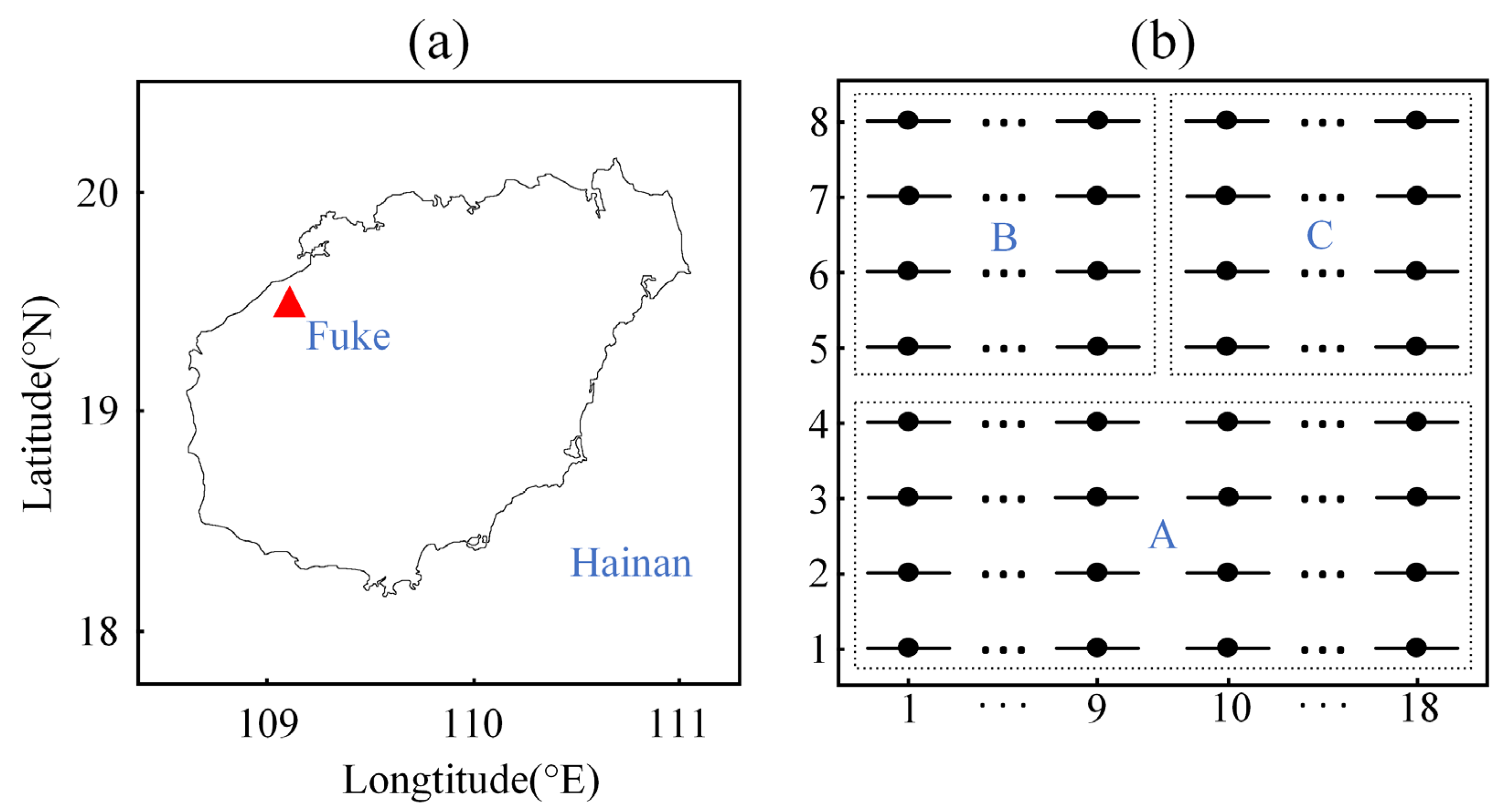
The HCOPAR is located at Fuke, northwest of Hainan Island of China (19.5°N, 109.1°E), which is marked with a triangle in Figure 1a. The operating frequency of the radar is 47 MHz, and it has a peak power of 54 kHz. As shown in array A in Figure 1b, the initial antenna array of the HCOPAR consists of 72 linearly polarized Yagi antennas arranged in an 18 × 4 matrix. The Yagi antennas are mounted at an inclination of 62.5° to the ground, so that the beam is perpendicular to the magnetic field lines in the ionosphere. The half-power beam width (HPBW) of the beam is 4.6° in the azimuth direction and 21.7° in the elevation direction [18]. After an upgrade in 2020, array B and array C arranged in a 9 × 4 matrix were added, and the two arrays were only used to receive the echoes. Array A was used for transmission as well as reception, and arrays B and C were employed only for reception. The space between the Yagi antenna elements is 0.7 times the wavelength. The phase center of array B is located 26.9 m northwest of array A, and the phase center of array C is located 40.2 m east of array B. With the interferometry technique, the angle of the meter-scale irregularities can be measured in the illuminating region [19]. The detection data collected by HCOPAR have a range resolution of 178 m and a temporal resolution of 20 s, and the detection range is 80–330 km. According to the layout of the antenna array, the interferometry equations for the HCOPAR can be developed to investigate the structures of the irregularities. It has been applied to study the daytime F-region irregularities using the interferometry technique at low latitudes in China [20].
The complex normalized cross-spectrum of two channel signals can be calculated as follows:
where VA(ω) and VB(ω) are the complex Fourier transforms of the signals received by array A and array B, respectively, and the asterisk denotes the complex conjugate; 〈〉 denotes the ensemble average; and SAB(ω) are the normalized cross-spectra of signals received by channel A and channel B. According to the complex cross-spectrum, the phase differences ∆ϕAB, ∆ϕBC, and ∆ϕAC can be obtained. The azimuth angle ϕ and the elevation angle θ of the scattering region can be derived as follows:
where β = 48.4°; l and m are the interferometry lobe numbers in the vertical and azimuth directions, respectively; and dAB and dBC are the distances between arrays A and B and B and C, respectively. Then, the scattering region can be constructed as follows:
where R is the slant range of the scattering region; Re is the Earth’s radius; and xeast, ynorth, and h are results in geomagnetic east, north, and vertical directions, respectively.
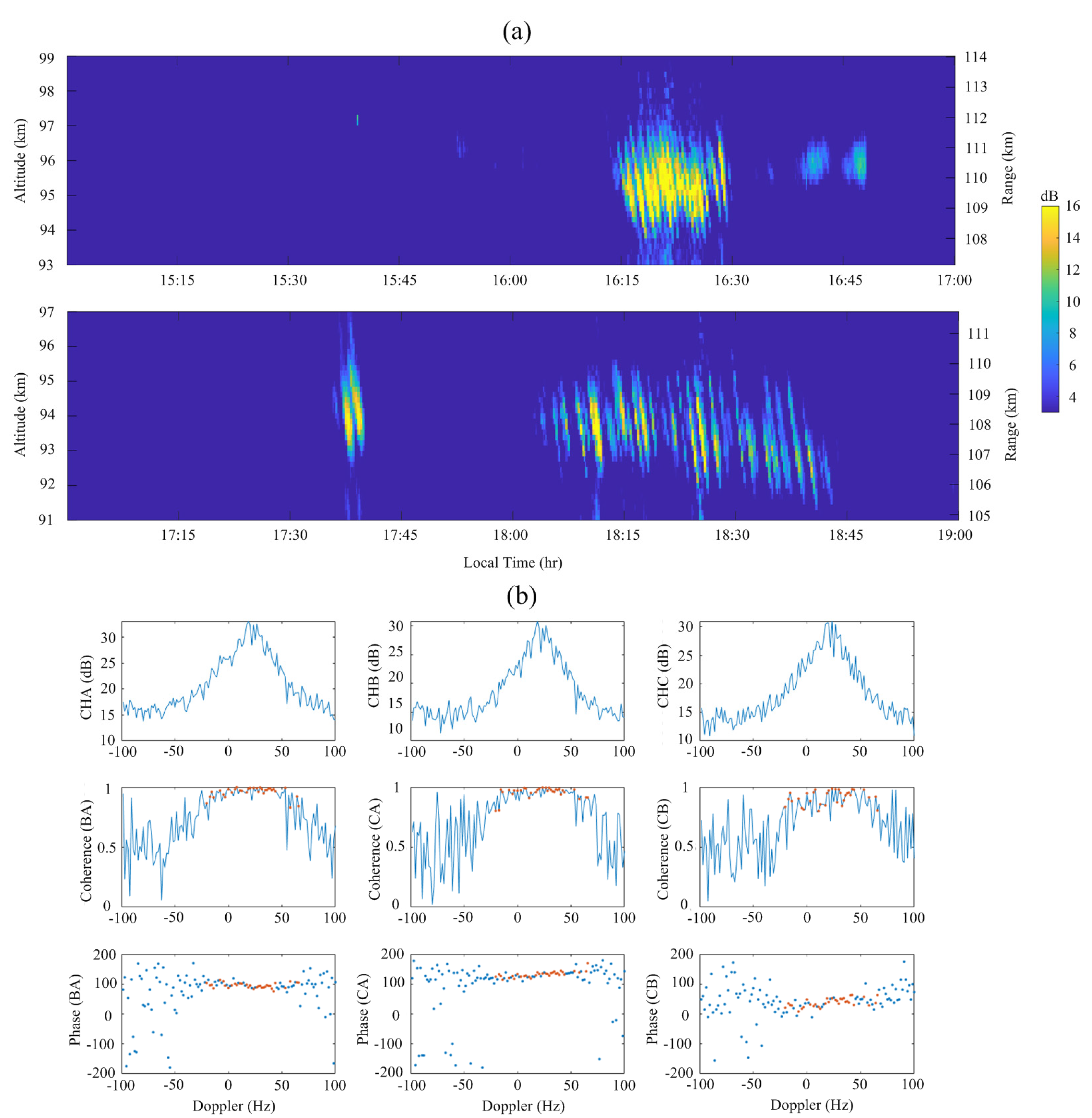
Figure 2a shows the height–time intensity (HTI) plot of the echoes observed using the HCOPAR during 15:00–19:00 LT on 12 March 2020. Because of the high magnetic aspect angle sensitivity of the field-aligned irregularities (FAIs) [21], the height information was obtained by multiplying the distance by the cosine (cos 29.75°) of the magnetic inclination of the E-layer in this region. The radar was operated with a 178 m range resolution and a 20 s temporal resolution, and the fine variation in the FAIs at the spatial and temporal scales could be observed. As shown in Figure 2a, there were two obvious LQP events. The first event was observed during 16:15–16:30 LT in the altitude range of 93.5–97 km, and the LQP structures had periods of about 64 s and a mean signal noise ratio (SNR) of 15 dB. The second event was observed during 18:00–18:50 LT in the altitude range of 91.5–95.5 km, and the LQP structures had periods of about 100 s and a mean SNR of 13.6 dB.
The pulse repetition frequency (PRF) of the radar is 200 Hz, and the non-coherent integration is 2. Thus, a group of 512 data points corresponds to a data length of 5.12 s. The repetition period of the cycle is 20 s for data acquisition and signal processing. The 128 points of the complex spectra were utilized to obtain the Doppler spectra for each channel. Before spectrum analysis with the fast Fourier transform (FFT), the 512 complex data points within 20 s were divided into four parts. The Doppler spectra of each receiver was analyzed two by two for the correlation spectra, and the four integrations were averaged to obtain the normalized correlation spectra. Taking the echoes at the range of 110 km during 16:17:10–16:17:30 LT as an example, Figure 2b shows the Doppler spectra and the cross-spectra for the three channels. The top panels show the Doppler spectra for each channel. The positive Doppler frequency denotes that the target is close to the radar. The middle and bottom panels show the coherence and phase of the same data. It can be found from Figure 2b that the phases are very close and concentrated around the spectral peak when the coherence is high and that phases with lower coherence have a random distribution. The spectral components with a high coherence indicate that the echoes from different channels come from the same scattering region. To ensure the quality of the echo reconstruction, the data with coherence greater than 0.8 and the phase difference of the three channels less than 3° were employed for the interferometry analysis, and the red points in the middle and bottom panels of Figure 2b met the requirements.
3. Analysis
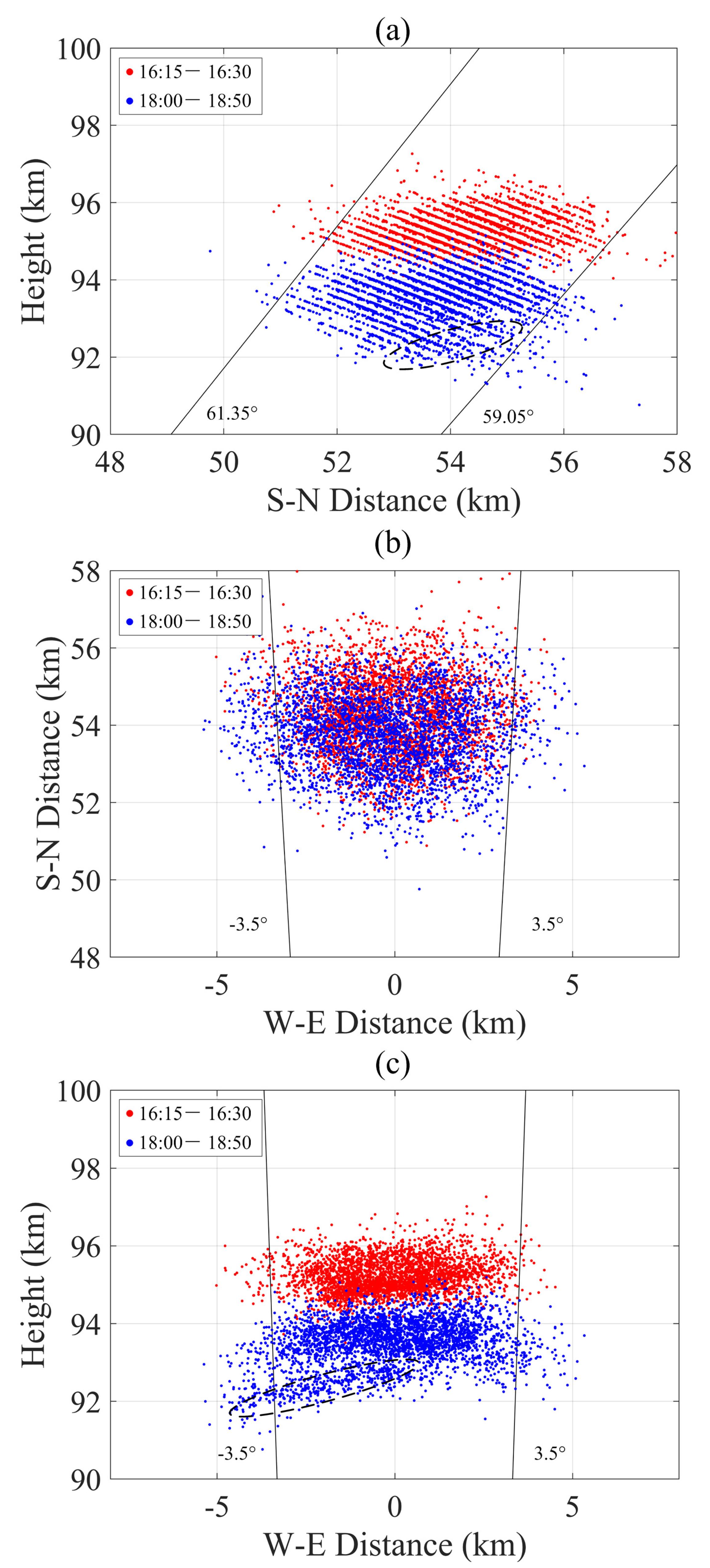
To further understand the characteristics of LQP echoes, we discuss the overall spatial distribution of the irregularities. The phase spectrum of each data set was extracted, and the echo points that met the above requirements were screened. After the phase correction, the points were projected on the mutually orthogonal planes to represent the echo regions. Figure 3a shows the echoes during 16:15–16:30 LT and 18:00–18:50 LT projected in the vertical plane by the vertical and the north–south axes, where the solid lines on the left and right indicate elevation angles of 61.35° and 59.05°, respectively. The red and blue points represent the echoes during 16:15–16:30 LT and 18:00–18:50 LT, respectively. The echo region during 16:15–16:30 LT had a scale of about 5 km in the north–south dimension and of about 2 km in the vertical dimension, which looks like a parallelogram in space. This indicates that the irregularities move in the north–south direction regularly. The echo region during 18:00–18:50 UT had a scale of about 3 km in the vertical dimension, which is an irregular shape in space. The abnormal region is highlighted by black dashed lines, and it indicates that there are irregularities moving abnormally. Meanwhile, we found that the LQP structures were distributed in strips, which indicates that the LQP structures were distributed along the magnetic lines. Figure 3b shows the projections of the echoes in the horizontal plane, where the solid lines on the left and right indicate an azimuth angle of –3.5° and 3.5°, respectively. Different from the oblique stripes in Figure 3a, the echoes were randomly distributed in the region with a scale of about 8 km in the east–west dimension. Most of the echoes had azimuth angles within 7°, which is larger than the half-power width of the main lobe (4.6°). Therefore, some echoes were received by the side lobe of the antenna. The echo regions during 16:15–16:30 LT and 18:00–18:50 LT were almost overlapping in the horizontal plane, which indicates that the irregularities in the two time periods were generated in the same region. Figure 3c shows the echoes projected in the vertical plane by the vertical and the east–west axes. The echo regions during 16:15–16:30 LT and 18:00–18:50 LT had almost the same scales in the north–south dimension and the vertical dimension, except the abnormal region highlighted by black dashed lines in the height range of 91.8–93 km. The height was the same as that of the abnormal region in Figure 3a, and we will discuss the anomaly region further.
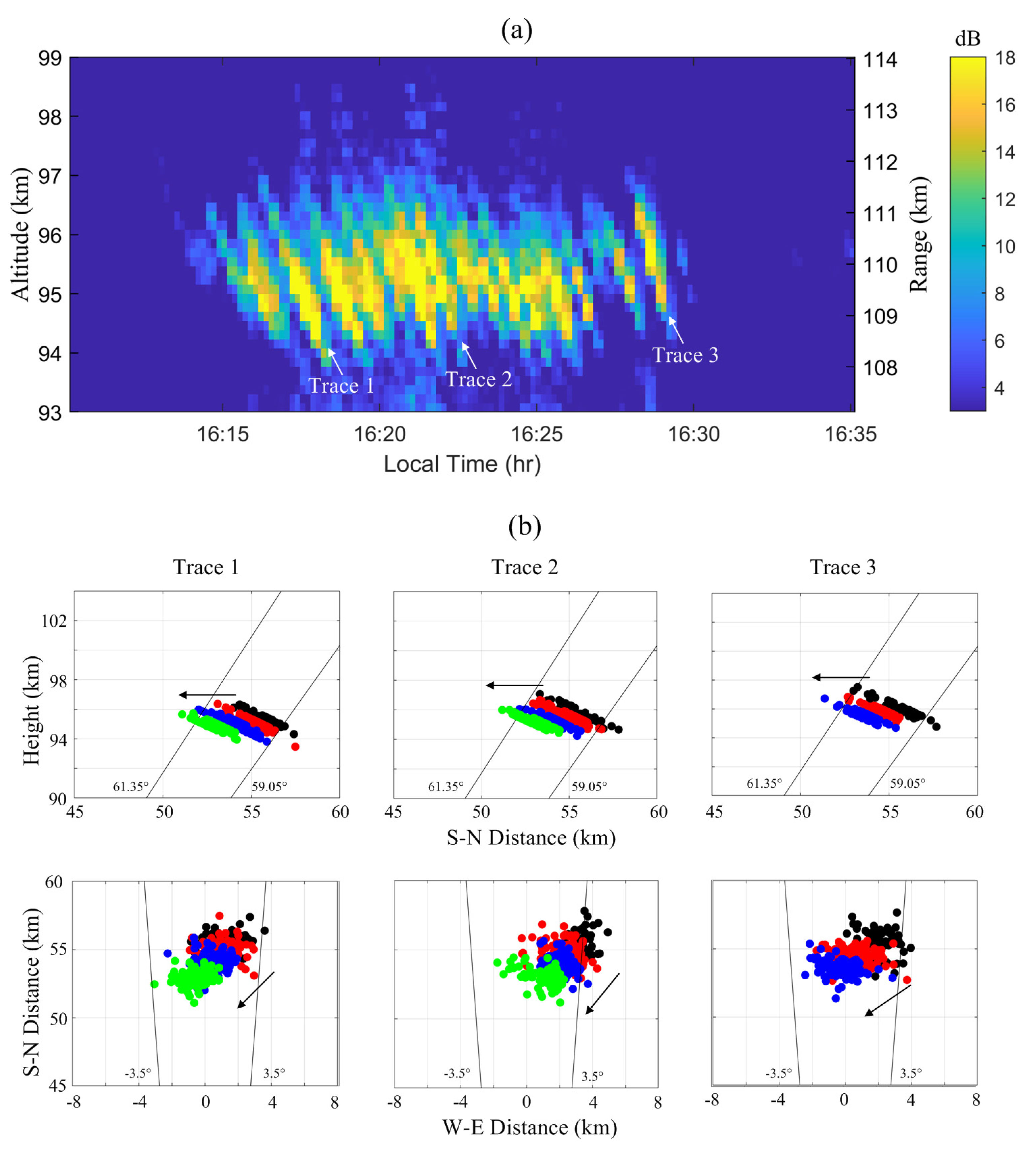
Figure 4a shows the LQP echoes observed during 16:15–16:30 LT. There were 14 significant LQP striations, with a height extension of 1 to 2 km and a period of about 64 s. The event lasted about 15 min, and all the striations had a negative slope. During the SEEK-2 campaign, the comparison of echoes obtained using the LTPR and the FAR revealed that echoing regions drifted with a southward velocity component, and the interferometry observation of the LTPR revealed that the negative range rate of the QP striations corresponded to a westward velocity component for the moving echoing regions [22]. Urbina et al. showed that the backscattering regions drifted in the westward direction [7], but Pan et al. found that a northwest to southeast drifting motion dominated within a preferential area [8]. To confirm what was happening in the case of the LQP structures, we tracked the positions of the LQP striations. The spatial structure of the LQP striations was reconstructed depending on the angular positions of the FAIs in the echoing region. To distinguish the state of each striation, we selected different colors to represent the spatial distributions of the irregularities at different times, and the arrows indicate the drifting direction of the LQP structures. Figure 4b shows the continuous changes in the spatial distributions for typical traces 1, 2, and 3 on the orthogonal planes. The plasma structures in traces 1, 2, and 3 moved southward at a trace velocity of about 44.0, 41.6, and 51.5 m/s, respectively. The plasma structures in traces 1, 2, and 3 moved downward at a trace velocity of about 8.3, 11.0, and 10.9 m/s, respectively, so they moved at an almost constant altitude. The plasma structures in traces 1, 2, and 3 moved westward at a trace velocity of about 26.8, 38.0, and 62.3 m/s, respectively. Therefore, the LQP structures in the three traces drifted southwestward almost horizontally. Due to the high aspect sensitivity, the plasma structures could only be observed in the elevation range of 59.05°–61.35°, so the plasma structures drifted into and out of the radar volume to form the LQP striations in the HTI plot.
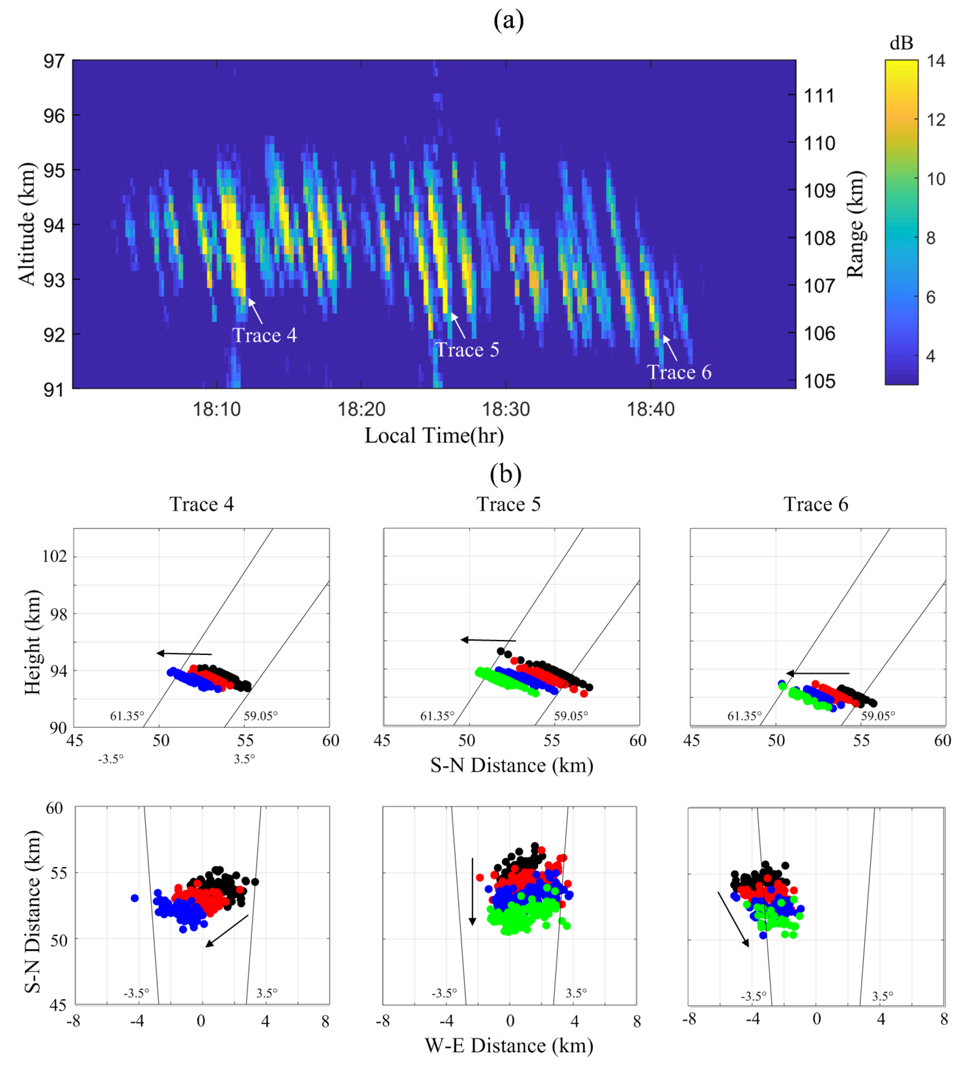
Figure 5a shows the LQP echoes observed during 18:00–18:50 LT. There were 25 significant LQP striations, with a height extension of 1 to 3 km and a period of about 96 s. The event lasted about 40 min, and all the striations had a negative slope. Figure 5b shows the continuous changes in the spatial distributions for typical traces 4, 5, and 6 on the orthogonal planes. The plasma structures in traces 4, 5, and 6 moved southward at a trace velocity of about 45.1, 53.9, and 50.1 m/s, respectively. The meridional velocity was close to the observed velocity during 16:15–16:30 LT, which indicates that the meridional wind was almost constant. As shown in Figure 5b, the plasma structures in trace 4 drifted westward at a trace velocity of about 60.0 m/s, which is similar to the case for traces 1, 2, and 3. However, the plasma structures in trace 5 and 6 drifted eastward at a trace velocity of about 0.3 and 15.4 m/s, respectively. Therefore, the latitudinal motion of the plasma structures in the striations during 18:00–18:50 LT was more complex. According to what has been discussed above, the plasma structures in the striations with a negative slope mainly drifted southwestward, but they also drifted southeastward in some striations. This indicates that there was less variation in the meridional winds and more variation in the latitudinal winds. Therefore, the abnormal region in Figure 3 was mainly induced by the eastward plasma structures.
4. Discussion
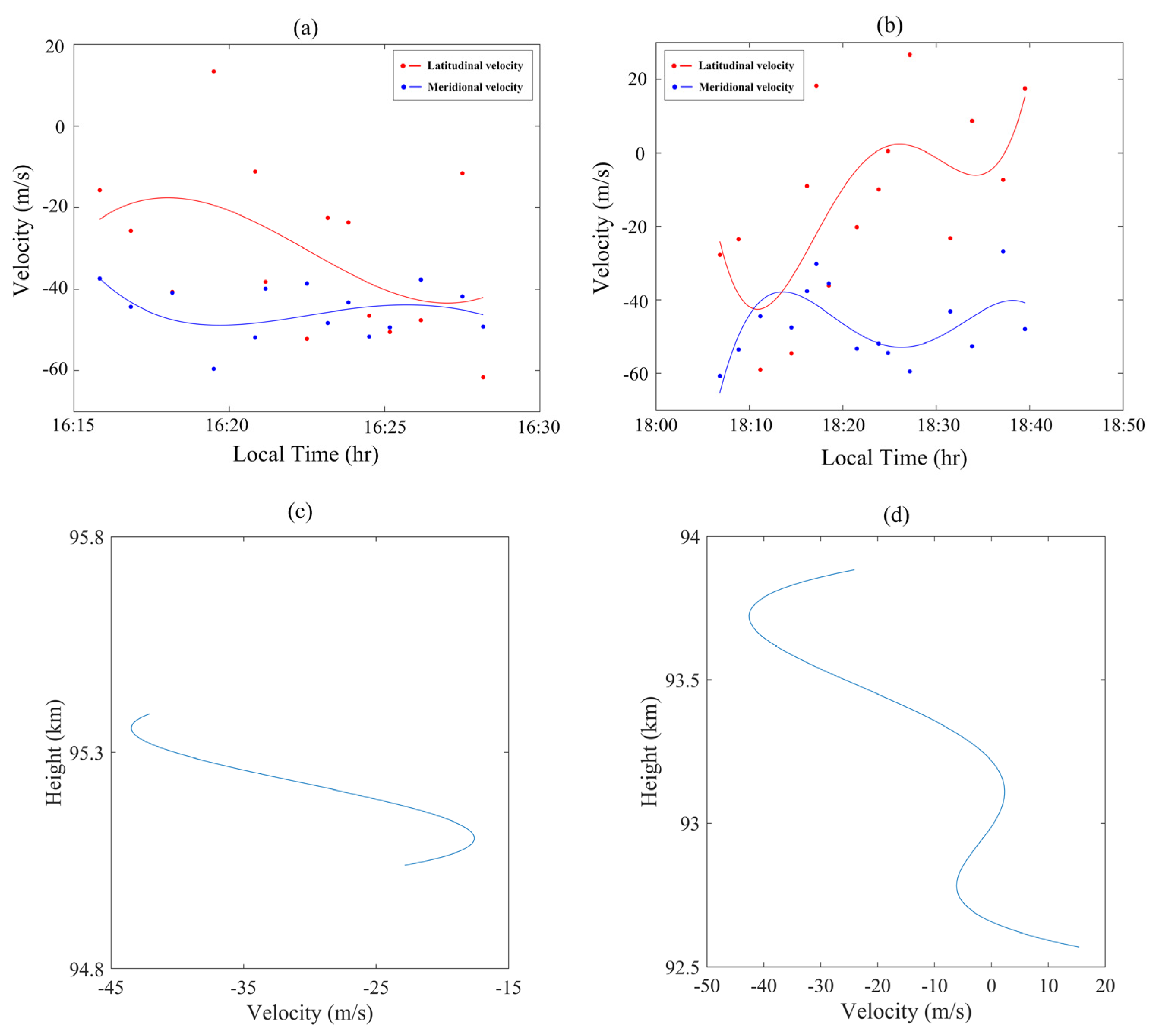
The interferometry investigations of the LQP echoes can help us discuss two questions. One is regarding the relationship between the negative slope of the LQP echoes and the movement of the plasma structures. The other is about what factors are associated with the different periodicities of the two events. According to the changes in the spatial distributions for each striation, the mean projection velocities in the latitudinal and meridional directions of different striations can be calculated. Figure 6a shows the results during 16:15–16:30 LT, and Figure 6b shows the results during 18:05–18:40 LT. The red and blue dots and lines indicate latitudinal and longitudinal velocities, respectively, and the lines are the results of fitting the points. It should be noted that some striations with a low SNR were deleted. The mean latitudinal velocities of the striations during 16:15–16:30 LT and 18:05–18:40 LT were 45.3 m/s and 46.6 m/s, and the mean latitudinal velocities were 31.0 m/s and 13.3 m/s. The meridional velocities were closer in the two time periods, while the differences in latitudinal velocities were larger. The similarity in the morphology of the LQP echoes in these two time periods was the negative slope, while the difference was the periodicity. Therefore, the southward wind might induce a negative slope. This is consistent with the statistical analysis of Chen et al. [16]. The latitudinal wind might be an important cause of the different periodicities in these two time periods.
In order to gain a deeper understanding of the LQP echoes’ generation mechanism, we further analyzed the data. Figure 6c,d display the height variations in the plasma structures’ latitudinal velocities during 16:15–16:30 LT and 18:05–18:40 LT. The trace velocity of the patch reflects the background wind velocity in the collision-dominated lower E-region (<100 km). As shown in Figure 6c,d, there were significant shears in the latitudinal velocities of the plasma structures. The shear during 16:15–16:30 LT was 101 (m/s)/km, and the shear during 18:05–18:40 LT was 50 (m/s)/km. The results indicate that there were neutral wind shears in the region in which the LQP echoes were produced, and the wind shear during 16:15–16:30 LT was larger than that during 18:05–18:40 LT. In previous studies, researchers have generally assumed that the neutral-wind-shear-driven Kelvin–Helmholtz instability (KHI) accounts for the LQP echoes [10]. This result is consistent with that assumption. The long-lived metallic ions from meteor ablation and deposition are converged by the wind shear to from a thin layer under the effect of the Earth’s magnetic field [23,24]. When the Richardson number, Ri, is <0.25, the thin layer becomes unstable due to KHI [25]. The KH billows associated with the instability produce the horizontal plasma density structures [5]. The plasma density structures embedded in the background wind can produce the QP striations when they drift into and out of the radar volume. Pan et al. reported that the striation periodicity of the QP echoes was related to the mean velocity in the unstable shear layer, i.e., the range rate velocity [26]. We found that the velocity shear during 16:15–16:30 LT was twice that during 18:05–18:40 LT, while the striation periodicity during 16:15–16:30 LT was half that during 18:05–18:40 LT. This means that the striation periodicity is inversely related to the wind shear. Therefore, the periodicity of the striations is more likely related to the strength of the wind shear.
5. Conclusions
In this article, we present high-resolution measurements of the LQP echoes observed with the upgraded HCOPAR. Two events were observed during 16:15–16:30 LT and 18:00–18:50 LT on 12 March 2020, and they had a negative slope and different periodicities. With the interferometry technique, we can investigate the movement of the plasma structures. According to movement of the plasma structures, the plasma structures in the striations with a negative slope mainly drifted southwestward. The results show that the LQP echoes with a negative slope were mainly induced by the southward-drifting plasma structures. According to the changes in the spatial distributions for each striation, the height variations in the plasma structures’ velocities in the two events can be obtained. We found strong wind shears in the region where the LQP echoes were produced. By comparing the LQP echoes with different periodicities, we found that the periodicity of the LQP echoes was more likely related to the strength of the wind shear. The striation periodicity was inversely related to the wind shear. Therefore, the obvious wind shear phenomenon indicates that the KHI may produce horizontal plasma density structures resulting in LQP echoes. In the future, we will analyze more cases and combine data from multiple sources to study the LQP echoes and focus on the generation mechanism of LQP echoes.
Author Contributions
Conceptualization, L.Q. and G.C.; methodology L.Q.; investigation, L.Q.; validation, M.S.; formal analysis, C.Y.; resources, C.Y.; visualization, E.L. and J.W.; funding acquisition, L.Q. and G.C. All authors have read and agreed to the published version of the manuscript.
Funding
This project was supported by the National Natural Science Foundation of China (42274197), the Fundamental Research Funds for the Central Universities (2042023kf0200), the Specialized Research Fund for State Key Laboratories, and the Natural Science Foundation of Zhejiang Province under grant LQ22D040001.
Data Availability Statement
The HCOPAR data are obtained from the Chinese Meridian Project website: https://data.meridianproject.ac.cn (accessed on 4 May 2022).
Acknowledgments
We appreciate the editors and the anonymous reviewers for their insightful comments and suggestions to improve this paper.
Conflicts of Interest
The authors declare no conflict of interest.
References
- Yamamoto, M.; Fukao, S.; Woodman, R.F.; Ogawa, T.; Tsuda, T.; Kato, S. Mid-latitude E region field-aligned irregularities observed with the MU radar. J. Geophys. Res. Space Phys. 1991, 96, 15943–15949. [Google Scholar] [CrossRef]
- Urbina, J.; Kudeki, E.; Franke, S.J.; Gonzalez, S.; Zhou, Q.; Collins, S.C. 50 MHz radar observations of mid-latitude E-region irregularities at Camp Santiago, Puerto Rico. Geophys. Res. Lett. 2000, 27, 2853–2856. [Google Scholar] [CrossRef]
- Rao, P.B.; Yamamoto, M.; Uchida, A.; Hassenpflug, I.; Fukao, S. MU radar observations of kilometer-scale waves in the mid latitude lower E-region. Geophys. Res. Lett. 2000, 27, 3667–3670. [Google Scholar] [CrossRef]
- Patra, A.K.; Sripathi, S.; Kumar, V.S.; Rao, P.B. Evidence of kilometer-scale waves in the lower E region from high resolution VHF radar observations over Gadanki. Geophys. Res. Lett. 2002, 29, 1371–1374. [Google Scholar] [CrossRef]
- Pan, C.J.; Rao, P.B. Low altitude quasi-periodic radar echoes observed by the Gadanki VHF radar. Geophys. Res. Lett. 2002, 29, 251–254. [Google Scholar] [CrossRef]
- Sripathi, S.; Patra, A.K.; Sivakumar, V.; Rao, P.B. Shear instability as a source of the daytime quasi-periodic radar echoes observed by the Gadanki VHF radar. Geophys. Res. Lett. 2003, 30, 2149. [Google Scholar] [CrossRef]
- Urbina, J.; Kudeki, E.; Franke, S.J.; Zhou, Q. Analysis of a mid-latitude E-region LQP event observed during the Coqui 2 Campaign. Geophys. Res. Lett. 2004, 31, 805. [Google Scholar] [CrossRef]
- Pan, C.J.; Röttger, J.; Chen, C.L. Radar investigations of low-altitude quasi-periodic echoes in Chung-Li. Geophys. Res. Lett. 2005, 32, 102. [Google Scholar] [CrossRef]
- Patra, A.K.; Sripathi, S.; Rao, P.B.; Choudhary, R.K. Gadanki radar observations of daytime E region echoes and structures extending down to 87 km. Ann. Geophys. 2006, 24, 1861–1869. [Google Scholar] [CrossRef]
- Patra, A.K.; Rao, N.V.; Choudhary, R.K. Daytime low-altitude quasi-periodic echoes at Gadanki: Understanding of their generation mechanism in the light of their Doppler characteristics. Geophys. Res. Lett. 2008, 36, L05107. [Google Scholar] [CrossRef]
- Venkateswara, N.V.; Patra, A.K.; Pant, T.K.; Rao, S.V.B. Morphology and seasonal characteristics of low latitude E-region quasiperiodic echoes studied using large database of Gadanki radar observations. J. Geophys. Res. Space Phys. 2008, 13, A07312. [Google Scholar] [CrossRef]
- Ning, B.; Li, G.; Hu, L.; Li, M. Observations on the field-aligned irregularities using Sanya VHF radar: 1. Ionospheric E-region continuous echoes. Chin. J. Geophys. 2013, 56, 719–730. (In Chinese) [Google Scholar]
- Li, G.; Ning, B.; Patra, A.K.; Wan, W.; Hu, L. Investigation of low-latitude E and valley region irregularities: Their relationship to equatorial plasma bubble bifurcation. J. Geophys. Res. Space Phys. 2011, 116, 11319. [Google Scholar] [CrossRef]
- Li, G.; Ning, B.; Patra, A.K.; Abdu, M.A.; Chen, J.; Liu, L.; Hu, L. On the linkage of daytime 150 km echoes and abnormal intermediate layer traces over Sany. J. Geophys. Res. Space Phys. 2013, 118, 7262–7267. [Google Scholar] [CrossRef]
- Li, G.; Ning, B.; Hu, L.; Li, M. Observations on the field-aligned irregularities using Sanya VHF radar: 2. Low latitude Ionospheric E-region quasi-periodic echoes in the East Asian sector. Chin. J. Geophys. 2013, 56, 2141–2151. (In Chinese) [Google Scholar]
- Chen, G.; Jin, H.; Huang, X.; Zhong, D.; Yan, C.; Yang, G. Strong correlation between quasiperiodic echoes and plasma drift in the E region. J. Geophys. Res. Space Phys. 2015, 120, 9110–9116. [Google Scholar] [CrossRef]
- Xie, H.; Li, G.; Zhao, X.; Ding, F.; Yan, C.; Yang, G.; Ning, B. Coupling Between E Region Quasi-Periodic Echoes and F Region Medium-Scale Traveling Ionospheric Disturbances at Low Latitudes. J. Geophys. Res. Space Phys. 2020, 125, A027720. [Google Scholar] [CrossRef]
- Chen, G.; Jin, H.; Yan, J.; Cui, X.; Zhang, S.; Yan, C.; Yang, G.-T.; Lan, A.-L.; Gong, W.-L.; Qiao, L.; et al. Hainan coherent scatter phased array radar (HCOPAR): System design and ionospheric irregularity observations. IEEE Trans. Geosci. Remote Sens. 2017, 55, 4757–4765. [Google Scholar] [CrossRef]
- Wang, C.Y.; Chu, Y.H.; Su, C.L.; Kuong, R.-M.; Chen, H.-C.; Yang, K.F. Statistical investigations of layer-type and clump-type plasma structures of 3-m field-aligned irregularities in nighttime sporadic e region made with chung-li vhf radar. J. Geophys. Res. Space Phys. 2011, 116, A12311. [Google Scholar] [CrossRef]
- He, Z.; Chen, G.; Yan, C.; Zhang, S.; Yang, G.; Li, Y.; Gong, W.; Wang, J.; Zhang, M. Imaging Radar Observations of the Daytime F-Region Irregularities in Low-Latitudes of China. J. Geophys. Res. Space Phys. 2023, 128, e2022JA030878. [Google Scholar] [CrossRef]
- Riggin, D.; Swartz, W.E.; Providakes, J.; Farley, D.T. Radar studies of long wavelength waves associated with mid latitude sporadic E layers. J. Geophys. Res. 1986, 91, 8011–8024. [Google Scholar] [CrossRef]
- Saito, S.; Yamamoto, M.; Fukao, S.; Marumoto, M.; Tsunoda, R.T. Radar observations of field-aligned plasma irregularities in the seek-2 campaign. Ann. Geophys. 2005, 23, 2307–2318. [Google Scholar] [CrossRef]
- Mathews, J.D. Sporadic-E: Current views and recent progress. J. Atmos. Sol. Terr. Phys. 1998, 60, 413–435. [Google Scholar] [CrossRef]
- Wang, J.; Zuo, X.; Sun, Y.-Y.; Yu, T.; Wang, Y.; Qiu, L.; Mao, T.; Yan, X.; Yang, N.; Qi, Y.; et al. Multilayered sporadice response to the annular solar eclipse on 21 June 2020. Space Weather 2021, 19, e2020SW002643. [Google Scholar] [CrossRef]
- Larsen, M.F. A shear instability seeding mechanism for quasi-periodic radar echoes. J. Geophys. Res. 2000, 105, 931–940. [Google Scholar]
- Pan, C.J.; Larsen, M.F. Observations of qp radar echo structure consistent with neutral wind shear control of the initiation mechanism. Geophys. Res. Lett. 2000, 27, 867–870. [Google Scholar] [CrossRef]
Figure 1.
(a) The location and (b) the layout of the antenna array of the upgraded HCOPAR. A, B, and C represent three subarrays.
Figure 1.
(a) The location and (b) the layout of the antenna array of the upgraded HCOPAR. A, B, and C represent three subarrays.

Figure 2.
(a) The HTI plot of the echoes observed using the HCOPAR during 15:00–19:00 LT on 12 March 2020. (b) Examples of the Doppler spectra, coherence, and phase of the echoes at a range of 110 km during 16:17:10–16:17:30 LT.
Figure 2.
(a) The HTI plot of the echoes observed using the HCOPAR during 15:00–19:00 LT on 12 March 2020. (b) Examples of the Doppler spectra, coherence, and phase of the echoes at a range of 110 km during 16:17:10–16:17:30 LT.

Figure 3.
(a) The echoes during 16:15–16:30 LT and 18:00–18:50 LT projected in the vertical plane by the vertical and north–south axes. (b) The echoes projected in the horizontal plane by the north–south and east–west axes. (c) The echoes projected in the vertical plane by the vertical and east–west axes.

Figure 4.
(a) The LQP echoes observed during 16:15–16:30 LT. (b) The continuous changes in the spatial distributions for traces 1, 2, and 3 on the orthogonal planes.
Figure 4.
(a) The LQP echoes observed during 16:15–16:30 LT. (b) The continuous changes in the spatial distributions for traces 1, 2, and 3 on the orthogonal planes.

Figure 5.
(a) The LQP echoes observed during 18:00–18:50 LT. (b) The continuous changes in the spatial distributions for traces 4, 5, and 6 on the orthogonal planes.
Figure 5.
(a) The LQP echoes observed during 18:00–18:50 LT. (b) The continuous changes in the spatial distributions for traces 4, 5, and 6 on the orthogonal planes.

Figure 6.
The mean projection velocities in the latitudinal and meridional directions of the striations during (a) 16:15–16:30 LT and (b) 18:05–18:40 LT. The height variations in the plasma structures’ latitudinal velocities during (c) 16:15–16:30 LT and (d) 18:05–18:40 LT.
Figure 6.
The mean projection velocities in the latitudinal and meridional directions of the striations during (a) 16:15–16:30 LT and (b) 18:05–18:40 LT. The height variations in the plasma structures’ latitudinal velocities during (c) 16:15–16:30 LT and (d) 18:05–18:40 LT.

Disclaimer/Publisher’s Note: The statements, opinions and data contained in all publications are solely those of the individual author(s) and contributor(s) and not of MDPI and/or the editor(s). MDPI and/or the editor(s) disclaim responsibility for any injury to people or property resulting from any ideas, methods, instructions or products referred to in the content. |
© 2023 by the authors. Licensee MDPI, Basel, Switzerland. This article is an open access article distributed under the terms and conditions of the Creative Commons Attribution (CC BY) license (https://creativecommons.org/licenses/by/4.0/).
Share and Cite
MDPI and ACS Style
Qiao, L.; Chen, G.; Su, M.; Yan, C.; Liu, E.; Wu, J. Analysis of the E-Region Low-Altitude Quasi-Periodic Event in Low-Latitudes of China. Remote Sens. 2023, 15, 5482. https://doi.org/10.3390/rs15235482
AMA Style
Qiao L, Chen G, Su M, Yan C, Liu E, Wu J. Analysis of the E-Region Low-Altitude Quasi-Periodic Event in Low-Latitudes of China. Remote Sensing. 2023; 15(23):5482. https://doi.org/10.3390/rs15235482
Chicago/Turabian StyleQiao, Lei, Gang Chen, Mingkun Su, Chunxiao Yan, Erxiao Liu, and Jun Wu. 2023. "Analysis of the E-Region Low-Altitude Quasi-Periodic Event in Low-Latitudes of China" Remote Sensing 15, no. 23: 5482. https://doi.org/10.3390/rs15235482
Note that from the first issue of 2016, this journal uses article numbers instead of page numbers. See further details here.