


Estimating the Surface Fuel Load of the Plant Physiognomy of the Cerrado Grassland Using Landsat 8 OLI Products
 , , ,
, , ,
Abstract
:1. Introduction
- (1)
- To evaluate the performance of multiple linear regression equations adjusted for load estimation in classes of live and dead fine fuels, considering the beginning and end of the dry season, based on the reflectance of Landsat 8 OLI images, vegetation indices, and fraction values (F-values) of the spectral mixture analysis (SMA);
- (2)
- To assess the use of random forest and k-nearest neighbor algorithms to estimate the fine fuel load in different classes in comparison to traditional multiple linear regression analyses;
- (3)
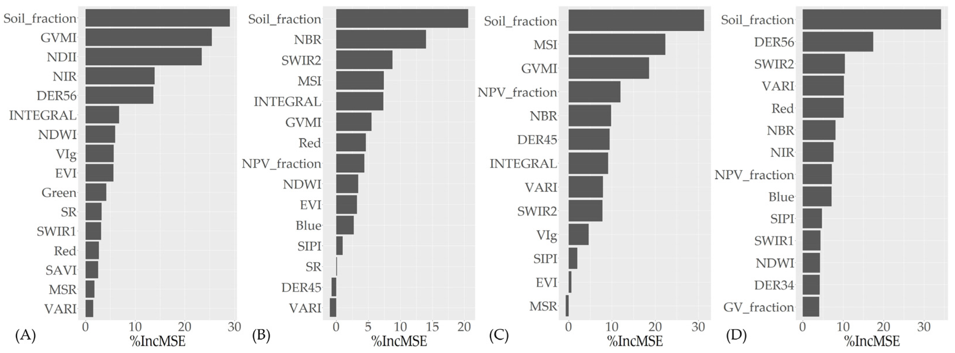
- To analyze the importance of each predictor variable from remote sensing products in random forest models.
2. Materials and Methods
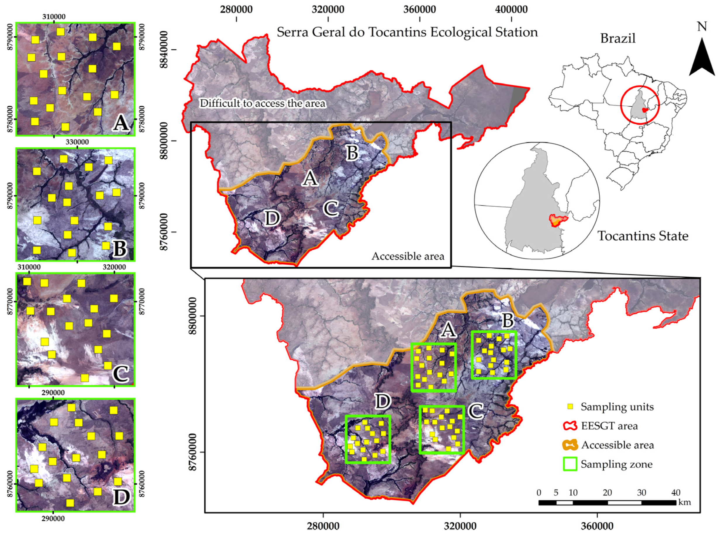
2.1. Study Area
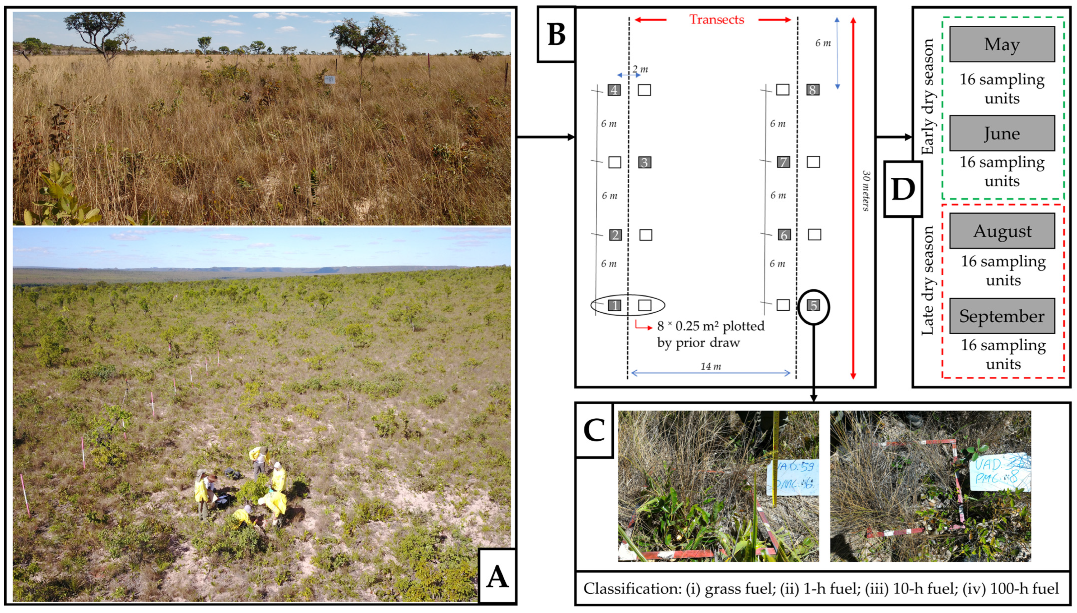
2.2. Field Survey
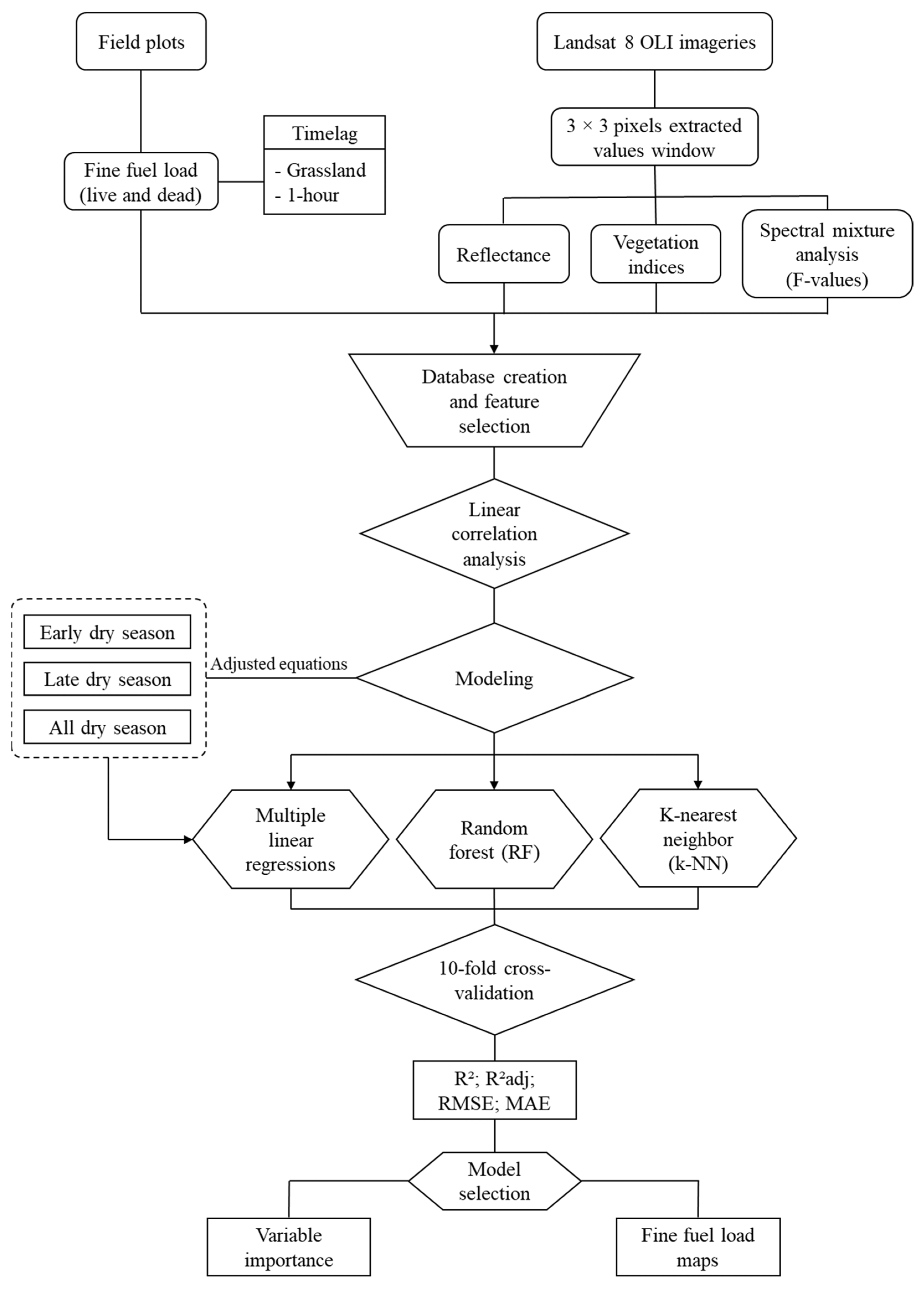
2.3. Obtaining and Processing Satellite Imagery
2.3.1. Vegetation Indices (VIs)
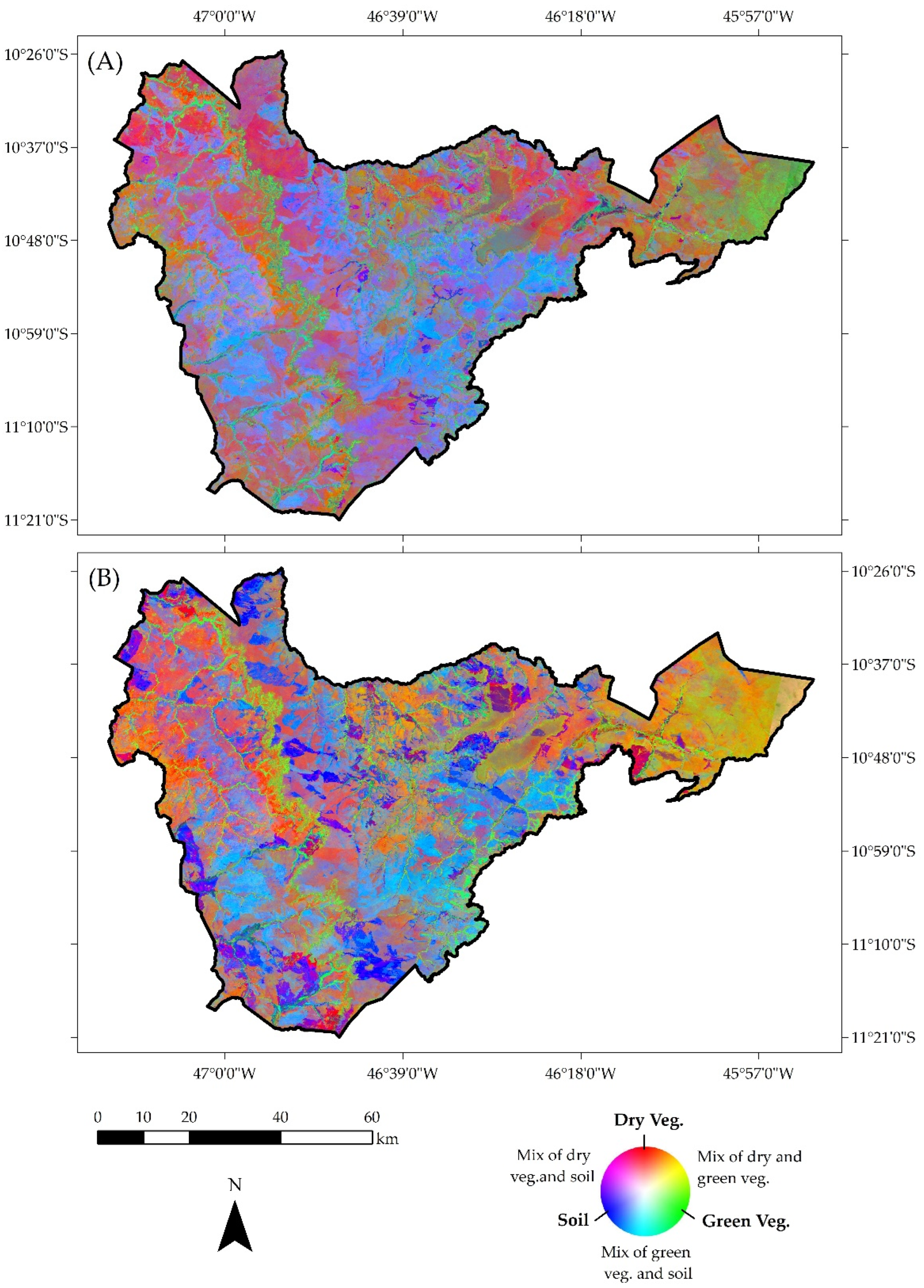
2.3.2. Spectral Mixture Analysis (SMA)
2.3.3. Data Extraction
2.4. Statistical Analysis of the Data
2.4.1. Multiple Linear Regression Analysis
2.4.2. Random Forest Machine Learning Algorithm
2.4.3. K-Nearest Neighbor Machine Learning Algorithm
2.4.4. Cross-Validation
3. Results
3.1. Multiple Linear Regression Analysis
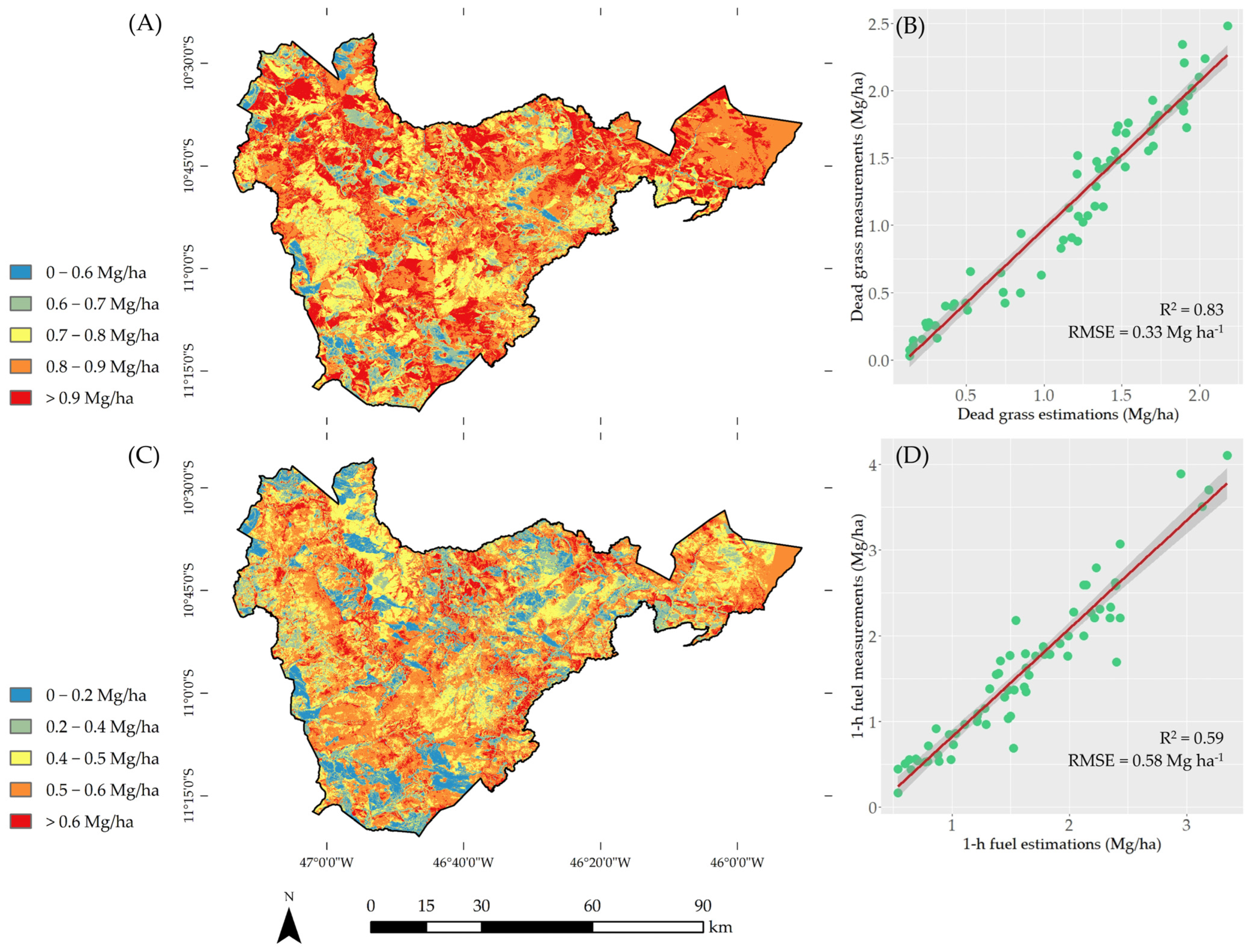
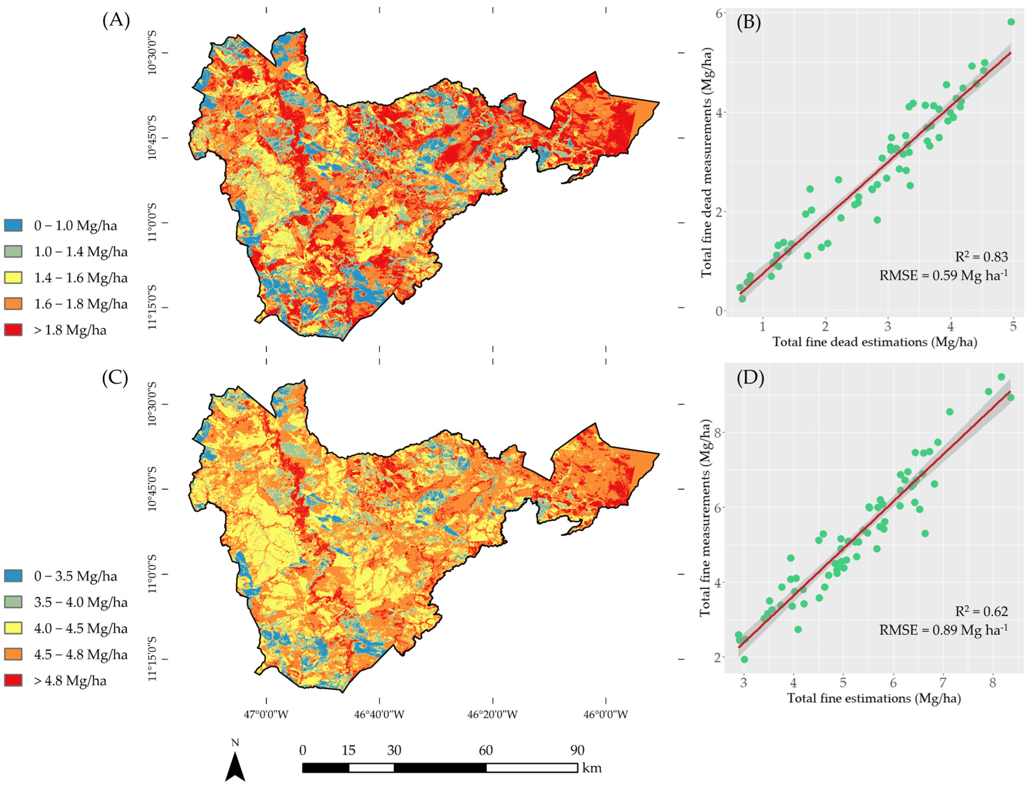
3.2. Estimates Using the Random Forest Algorithm
3.2.1. Model Performance Metrics
3.2.2. Importance of the Variables in the Random Forest Models
3.3. Estimates using the K-Nearest Neighbor Algorithm
4. Discussion
5. Conclusions
Author Contributions
Funding
Data Availability Statement
Acknowledgments
Conflicts of Interest
References
- Miranda, H.S.; Sato, M.N.; Neto, W.N.; Aires, F.S. Fires in the Cerrado, the Brazilian Savanna. Trop. Fire Ecol. 2009, 427–450. [Google Scholar] [CrossRef]
- Brown, J.K.; Oberheu, R.D.; Johnston, C.M. Handbook for Inventorying Surface Fuels and Biomass in the Interior West; Gen. Tech. Rep. INT-129; U.S. Department of Agriculture: Washington, DC, USA; Forest Service: Washington, DC, USA; Intermountain Forest and Range Experimental Station: Washington, DC, USA, 1982; Volume 129, 48p. [CrossRef]
- Rothermel, R.C. A Mathematical Model for Predicting Fire Spread in Wildland Fuels; Intermountain Forest & Range Experiment Station: Washington, DC, USA; Forest Service: Washington, DC, USA; US Department of Agriculture, USDA: Washington, DC, USA, 1972; pp. 1–48.
- Keane, R.E.; Herynk, J.M.; Toney, C.; Urbanski, S.P.; Lutes, D.C.; Ottmar, R.D. Evaluating the Performance and Mapping of Three Fuel Classification Systems Using Forest Inventory and Analysis Surface Fuel Measurements. For. Ecol. Manag. 2013, 305, 248–263. [Google Scholar] [CrossRef]
- Kanmegne Tamga, D.; Latifi, H.; Ullmann, T.; Baumhauer, R.; Bayala, J.; Thiel, M. Estimation of Aboveground Biomass in Agroforestry Systems over Three Climatic Regions in West Africa Using Sentinel-1, Sentinel-2, ALOS, and GEDI Data. Sensors 2023, 23, 349. [Google Scholar] [CrossRef]
- Li, Z.; Angerer, J.P.; Jaime, X.; Yang, C.; Wu, X. Ben Estimating Rangeland Fine Fuel Biomass in Western Texas Using High-Resolution Aerial Imagery and Machine Learning. Remote Sens. 2022, 14, 4360. [Google Scholar] [CrossRef]
- Roberts, D.A.; Dennison, P.E.; Gardner, M.E.; Hetzel, Y.; Ustin, S.L.; Lee, C.T. Evaluation of the Potential of Hyperion for Fire Danger Assessment by Comparison to the Airborne Visible/Infrared Imaging Spectrometer. IEEE Trans. Geosci. Remote Sens. 2003, 41, 1297–1310. [Google Scholar] [CrossRef]
- Kukavskaya, E.A.; Shvetsov, E.G.; Buryak, L.V.; Tretyakov, P.D.; Groisman, P.Y. Increasing Fuel Loads, Fire Hazard, and Carbon Emissions from Fires in Central Siberia. Fire 2023, 6, 63. [Google Scholar] [CrossRef]
- Szpakowski, D.M.; Jensen, J.L.R. A Review of the Applications of Remote Sensing in Fire Ecology. Remote Sens. 2019, 11, 2638. [Google Scholar] [CrossRef]
- van Wagtendonk, J.W.; Root, R.R. The Use of Multi-Temporal Landsat Normalized Difference Vegetation Index (NDVI) Data for Mapping Fuel Models in Yosemite National Park, USA. Int. J. Remote Sens. 2010, 24, 1639–1651. [Google Scholar] [CrossRef]
- Ji, L.; Wylie, B.K.; Nossov, D.R.; Peterson, B.; Waldrop, M.P.; McFarland, J.W.; Rover, J.; Hollingsworth, T.N. Estimating Aboveground Biomass in Interior Alaska with Landsat Data and Field Measurements. Int. J. Appl. Earth Obs. Geoinf. 2012, 18, 451–461. [Google Scholar] [CrossRef]
- Frazier, R.J.; Coops, N.C.; Wulder, M.A.; Kennedy, R. Characterization of Aboveground Biomass in an Unmanaged Boreal Forest Using Landsat Temporal Segmentation Metrics. ISPRS J. Photogramm. Remote Sens. 2014, 92, 137–146. [Google Scholar] [CrossRef]
- Zhang, G.; Ganguly, S.; Nemani, R.R.; White, M.A.; Milesi, C.; Hashimoto, H.; Wang, W.; Saatchi, S.; Yu, Y.; Myneni, R.B. Estimation of Forest Aboveground Biomass in California Using Canopy Height and Leaf Area Index Estimated from Satellite Data. Remote Sens. Environ. 2014, 151, 44–56. [Google Scholar] [CrossRef]
- Bao, W.; Yu, F.; Chang, Y.; Guo, M.; Zhou, F.; Zhong, C. Estimation of Fuel Load Using Remote Sensing Data in Hulunbuir Grassland. Nat. Hazards Res. 2022, 2, 375–383. [Google Scholar] [CrossRef]
- Li, Y.; Quan, X.; Liao, Z.; He, B. Forest Fuel Loads Estimation from Landsat ETM+ and ALOS PALSAR Data. Remote Sens. 2021, 13, 1189. [Google Scholar] [CrossRef]
- Gao, X.; Dong, S.; Li, S.; Xu, Y.; Liu, S.; Zhao, H.; Yeomans, J.; Li, Y.; Shen, H.; Wu, S.; et al. Using the Random Forest Model and Validated MODIS with the Field Spectrometer Measurement Promote the Accuracy of Estimating Aboveground Biomass and Coverage of Alpine Grasslands on the Qinghai-Tibetan Plateau. Ecol. Indic. 2020, 112, 106114. [Google Scholar] [CrossRef]
- Cui, L.; Jiao, Z.; Dong, Y.; Sun, M.; Zhang, X.; Yin, S.; Ding, A.; Chang, Y.; Guo, J.; Xie, R. Estimating Forest Canopy Height Using MODIS BRDF Data Emphasizing Typical-Angle Reflectances. Remote Sens. 2019, 11, 2239. [Google Scholar] [CrossRef]
- Goldbergs, G.; Levick, S.R.; Lawes, M.; Edwards, A. Hierarchical Integration of Individual Tree and Area-Based Approaches for Savanna Biomass Uncertainty Estimation from Airborne LiDAR. Remote Sens. Environ. 2018, 205, 141–150. [Google Scholar] [CrossRef]
- Xu, Q.; Man, A.; Fredrickson, M.; Hou, Z.; Pitkänen, J.; Wing, B.; Ramirez, C.; Li, B.; Greenberg, J.A. Quantification of Uncertainty in Aboveground Biomass Estimates Derived from Small-Footprint Airborne LiDAR. Remote Sens. Environ. 2018, 216, 514–528. [Google Scholar] [CrossRef]
- Zarco-Tejada, P.J.; Rueda, C.A.; Ustin, S.L. Water Content Estimation in Vegetation with MODIS Reflectance Data and Model Inversion Methods. Remote Sens. Environ. 2003, 85, 109–124. [Google Scholar] [CrossRef]
- Dennison, P.E.; Roberts, D.A.; Peterson, S.H.; Rechel, J. Use of Normalized Difference Water Index for Monitoring Live Fuel Moisture. Int. J. Remote Sens. 2006, 26, 1035–1042. [Google Scholar] [CrossRef]
- Sousa, D.; Small, C. Global Cross-Calibration of Landsat Spectral Mixture Models. Remote Sens. Environ. 2017, 192, 139–149. [Google Scholar] [CrossRef]
- Routh, D.; Seegmiller, L.; Bettigole, C.; Kuhn, C.; Oliver, C.D.; Glick, H.B. Improving the Reliability of Mixture Tuned Matched Filtering Remote Sensing Classification Results Using Supervised Learning Algorithms and Cross-Validation. Remote Sens. 2018, 10, 1675. [Google Scholar] [CrossRef]
- Franke, J.; Barradas, A.C.S.; Borges, M.A.; Menezes Costa, M.; Dias, P.A.; Hoffmann, A.A.; Orozco Filho, J.C.; Melchiori, A.E.; Siegert, F. Fuel Load Mapping in the Brazilian Cerrado in Support of Integrated Fire Management. Remote Sens. Environ. 2018, 217, 221–232. [Google Scholar] [CrossRef]
- Secretaria do Planejamento e da Modernização da Gestão Pública (Seplan). Atlas of Tocantins: Subsidies for Land Management Planning [Atlas Do Tocantins: Subsídios Ao Planejamento Da Gestão Territorial], 6th ed.; Governo do Estado do Tocantins: Palmas, Brazil, 2012.
- Instituto Chico Mendes De Conservação Da Biodiversidade (ICMBio). Management Plan for Serra Geral Do Tocantins Ecological Station [Plano de Manejo Para Estação Ecológica Serra Geral Do Tocantins (EESGT)], 1st ed.; Instituto Chico Mendes De Conservação Da Biodiversidade (ICMBio): Brasília, Brazil, 2014; Volume 1.
- Arruda, M.B.; von Behr, M. Jalapão: Scientific and Conservation Expedition [Jalapão: Expedição Científica e Conservacionista], 1st ed.; Instituto Brasileiro do Meio Ambiente e dos Recursos Naturais Renováveis (Ibama): Brasília, Brazil, 2002; Volume 1.
- Ribeiro, J.F.; Walter, B.M.T. The Main Phytophysiognomies of the Cerrado Biome [As Principais Fitofisionomias Do Bioma Cerrado]; Sano, S.M., Almeida, S.P., Ribeiro, J.F., Eds.; Embrapa: Brasília, Brazil, 2008; Volume 1.
- Santos, R.P.; Crema, A.; Szmuchrowski, M.A.; Possapp, J.J.; Nogueira, C.C.; Asano, K.; Kawaguchi, M.; Dino, K. Atlas of the Ecological Corridor of the Jalapão Region [Atlas Do Corredor Ecológico Da Região Do Jalapão], 2nd ed.; Instituto Chico Mendes de Conservação da Biodiversidade: Brasília, Brazil, 2013; Volume 1.
- Schroeder, M.J.; Buck, C.C. Fire Weather: A Guide for Application of Meteorological Information to Forest Fire Control Operations; USDA: Washington, DC, USA, 1970; Volume 1.
- Gorelick, N.; Hancher, M.; Dixon, M.; Ilyushchenko, S.; Thau, D.; Moore, R. Google Earth Engine: Planetary-Scale Geospatial Analysis for Everyone. Remote Sens. Environ. 2017, 202, 18–27. [Google Scholar] [CrossRef]
- Vermote, E.; Roger, J.C.; Franch, B.; Skakun, S. LASRC (Land Surface Reflectance Code): Overview, Application and Validation Using MODIS, VIIRS, LANDSAT and Sentinel 2 Data’s. In Proceedings of the IGARSS 2018-2018 IEEE International Geoscience and Remote Sensing Symposium (IGARSS), Valencia, Spain, 22–27 July 2018; pp. 8173–8176. [Google Scholar] [CrossRef]
- Davidson, A.; Wang, S.; Wilmshurst, J. Remote Sensing of Grassland–Shrubland Vegetation Water Content in the Shortwave Domain. Int. J. Appl. Earth Obs. Geoinf. 2006, 8, 225–236. [Google Scholar] [CrossRef]
- Yebra, M.; Dennison, P.E.; Chuvieco, E.; Riaño, D.; Zylstra, P.; Hunt, E.R.; Danson, F.M.; Qi, Y.; Jurdao, S. A Global Review of Remote Sensing of Live Fuel Moisture Content for Fire Danger Assessment: Moving towards Operational Products. Remote Sens. Environ. 2013, 136, 455–468. [Google Scholar] [CrossRef]
- Rouse, J.W.J.; Haas, R.H.; Schell, J.A.; Deering, D.W. Monitoring Vegetation Systems in the Great Plains with ERTS; NASA Technical Reports Server (NTRS): Hampton, VA, USA, 1974.
- Gitelson, A.A.; Kaufman, Y.J.; Stark, R.; Rundquist, D. Novel Algorithms for Remote Estimation of Vegetation Fraction. Remote Sens. Environ. 2002, 80, 76–87. [Google Scholar] [CrossRef]
- Birth, G.S.; McVey, G.R. Measuring the Color of Growing Turf with a Reflectance Spectrophotometer1. Agron. J. 1968, 60, 640–643. [Google Scholar] [CrossRef]
- Peñuelas, J.; Filella, I.; Gamon, J.A. Assessment of Photosynthetic Radiation-Use Efficiency with Spectral Reflectance. New Phytol. 1995, 131, 291–296. [Google Scholar] [CrossRef]
- Huete, A.R. A Soil-Adjusted Vegetation Index (SAVI). Remote Sens. Environ. 1988, 25, 295–309. [Google Scholar] [CrossRef]
- Gao, B.C. NDWI—A Normalized Difference Water Index for Remote Sensing of Vegetation Liquid Water from Space. Remote Sens. Environ. 1996, 58, 257–266. [Google Scholar] [CrossRef]
- Hunt, E.R.; Rock, B.N. Detection of Changes in Leaf Water Content Using Near- and Middle-Infrared Reflectances. Remote Sens. Environ. 1989, 30, 43–54. [Google Scholar] [CrossRef]
- Paltridge, G.W.; Barber, J. Monitoring Grassland Dryness and Fire Potential in Australia with NOAA/AVHRR Data. Remote Sens. Environ. 1988, 25, 381–394. [Google Scholar] [CrossRef]
- Chen, J.M. Evaluation of Vegetation Indices and a Modified Simple Ratio for Boreal Applications. Can. J. Remote Sens. 2014, 22, 229–242. [Google Scholar] [CrossRef]
- Rock, B.N.; Vogelmann, J.E.; Williams, D.L.; Vogelmann, A.F.; Hoshizaki, T. Remote Detection of Forest DamagePlant Responses to Stress May Have Spectral “Signatures” That Could Be Used to Map, Monitor, and Measure Forest Damage. Bioscience 1986, 36, 439–445. [Google Scholar] [CrossRef]
- Xu, H. Modification of Normalised Difference Water Index (NDWI) to Enhance Open Water Features in Remotely Sensed Imagery. Int. J. Remote Sens. 2007, 27, 3025–3033. [Google Scholar] [CrossRef]
- Chuvieco, E.; Martín, M.P.; Palacios, A. Assessment of Different Spectral Indices in the Red-near-Infrared Spectral Domain for Burned Land Discrimination. Int. J. Remote Sens. 2010, 23, 5103–5110. [Google Scholar] [CrossRef]
- Huete, A.R.; Liu, H.Q.; Batchily, K.; van Leeuwen, W. A Comparison of Vegetation Indices over a Global Set of TM Images for EOS-MODIS. Remote Sens. Environ. 1997, 59, 440–451. [Google Scholar] [CrossRef]
- Danson, F.M.; Steven, M.D.; Malthus, T.J.; Clark, J.A. High-Spectral Resolution Data for Determining Leaf Water Content. Int. J. Remote Sens. 1992, 13, 461–470. [Google Scholar] [CrossRef]
- Ozkan, S.; Bozdagi Akar, G. Improved Deep Spectral Convolution Network for Hyperspectral Unmixing With Multinomial Mixture Kernel and Endmember Uncertainty. arXiv 2018, arXiv:1808.01104. [Google Scholar]
- Cao, S.; Yu, Q.; Sanchez-Azofeifa, A.; Feng, J.; Rivard, B.; Gu, Z. Mapping Tropical Dry Forest Succession Using Multiple Criteria Spectral Mixture Analysis. ISPRS J. Photogramm. Remote Sens. 2015, 109, 17–29. [Google Scholar] [CrossRef]
- Mayes, M.T.; Mustard, J.F.; Melillo, J.M. Forest Cover Change in Miombo Woodlands: Modeling Land Cover of African Dry Tropical Forests with Linear Spectral Mixture Analysis. Remote Sens. Environ. 2015, 165, 203–215. [Google Scholar] [CrossRef]
- Richter, R. A Spatially Adaptive Fast Atmospheric Correction Algorithm. Int. J. Remote Sens. 1996, 17, 1201–1214. [Google Scholar] [CrossRef]
- Tane, Z.; Roberts, D.; Veraverbeke, S.; Casas, Á.; Ramirez, C.; Ustin, S. Evaluating Endmember and Band Selection Techniques for Multiple Endmember Spectral Mixture Analysis Using Post-Fire Imaging Spectroscopy. Remote Sens. 2018, 10, 389. [Google Scholar] [CrossRef]
- Crabbé, A.H.; Somers, B.; Roberts, D.A.; Halligan, K.; Dennison, P.; Dudley, K. MESMA QGIS Plugin (Version 1.0.8). 2020. Available online: https://mesma.readthedocs.io/ (accessed on 21 September 2023).
- Chuvieco, E.; Riaño, D.; Aguado, I.; Cocero, D. Estimation of Fuel Moisture Content from Multitemporal Analysis of Landsat Thematic Mapper Reflectance Data: Applications in Fire Danger Assessment. Int. J. Remote Sens. 2002, 23, 2145–2162. [Google Scholar] [CrossRef]
- Helmer, E.H.; Ruzycki, T.S.; Wunderle, J.M.; Vogesser, S.; Ruefenacht, B.; Kwit, C.; Brandeis, T.J.; Ewert, D.N. Mapping Tropical Dry Forest Height, Foliage Height Profiles and Disturbance Type and Age with a Time Series of Cloud-Cleared Landsat and ALI Image Mosaics to Characterize Avian Habitat. Remote Sens. Environ. 2010, 114, 2457–2473. [Google Scholar] [CrossRef]
- Main-Knorn, M.; Cohen, W.B.; Kennedy, R.E.; Grodzki, W.; Pflugmacher, D.; Griffiths, P.; Hostert, P. Monitoring Coniferous Forest Biomass Change Using a Landsat Trajectory-Based Approach. Remote Sens. Environ. 2013, 139, 277–290. [Google Scholar] [CrossRef]
- Chrysafis, I.; Mallinis, G.; Gitas, I.; Tsakiri-Strati, M. Estimating Mediterranean Forest Parameters Using Multi Seasonal Landsat 8 OLI Imagery and an Ensemble Learning Method. Remote Sens. Environ. 2017, 199, 154–166. [Google Scholar] [CrossRef]
- Marselis, S.M.; Tang, H.; Armston, J.D.; Calders, K.; Labrière, N.; Dubayah, R. Distinguishing Vegetation Types with Airborne Waveform Lidar Data in a Tropical Forest-Savanna Mosaic: A Case Study in Lopé National Park, Gabon. Remote Sens. Environ. 2018, 216, 626–634. [Google Scholar] [CrossRef]
- Breiman, L. Random Forests. Mach. Learn. 2001, 45, 5–32. [Google Scholar] [CrossRef]
- Zeng, N.; Ren, X.; He, H.; Zhang, L.; Zhao, D.; Ge, R.; Li, P.; Niu, Z. Estimating Grassland Aboveground Biomass on the Tibetan Plateau Using a Random Forest Algorithm. Ecol. Indic. 2019, 102, 479–487. [Google Scholar] [CrossRef]
- de Carvalho Junior, W.; Calderano Filho, B.; da Silva Chagas, C.; Bhering, S.B.; Pereira, N.R.; Pinheiro, H.S.K. Multiple Linear Regression and Random Forest Model to Estimate Soil Bulk Density in Mountainous Regions [Regressão Linear Múltipla e Modelo Random Forest Para Estimar a Densidade Do Solo Em Áreas Montanhosas]. Pesqui Agropecu Bras 2016, 51, 1428–1437. [Google Scholar] [CrossRef]
- Li, Z.; Xin, X.; Huan, T.; Fan, Y.; Chen, B.; Zhang, B. Estimating Grassland LAI Using the Random Forests Approach and Landsat Imagery in the Meadow Steppe of Hulunber, China. J. Integr. Agric. 2017, 16, 286–297. [Google Scholar] [CrossRef]
- Ou, Q.; Lei, X.; Shen, C. Individual Tree Diameter Growth Models of Larch–Spruce–Fir Mixed Forests Based on Machine Learning Algorithms. Forests 2019, 10, 187. [Google Scholar] [CrossRef]
- Thanh Noi, P.; Kappas, M. Comparison of Random Forest, k-Nearest Neighbor, and Support Vector Machine Classifiers for Land Cover Classification Using Sentinel-2 Imagery. Sensors 2018, 18, 18. [Google Scholar] [CrossRef] [PubMed]
- Wang, L.; Zhou, X.; Zhu, X.; Dong, Z.; Guo, W. Estimation of Biomass in Wheat Using Random Forest Regression Algorithm and Remote Sensing Data. Crop J. 2016, 4, 212–219. [Google Scholar] [CrossRef]
- Sun, H.; Gui, D.; Yan, B.; Liu, Y.; Liao, W.; Zhu, Y.; Lu, C.; Zhao, N. Assessing the Potential of Random Forest Method for Estimating Solar Radiation Using Air Pollution Index. Energy Convers. Manag. 2016, 119, 121–129. [Google Scholar] [CrossRef]
- Liaw, A.; Wiener, M. Classification and Regression by RandomForest. R News 2002, 2, 18–22. [Google Scholar]
- Gao, Y.; Lu, D.; Li, G.; Wang, G.; Chen, Q.; Liu, L.; Li, D. Comparative Analysis of Modeling Algorithms for Forest Aboveground Biomass Estimation in a Subtropical Region. Remote Sens. 2018, 10, 627. [Google Scholar] [CrossRef]
- Ohmann, J.L.; Gregory, M.J.; Roberts, H.M. Scale Considerations for Integrating Forest Inventory Plot Data and Satellite Image Data for Regional Forest Mapping. Remote Sens. Environ. 2014, 151, 3–15. [Google Scholar] [CrossRef]
- Zhang, W.; Zhao, L.; Li, Y.; Shi, J.; Yan, M.; Ji, Y. Forest Above-Ground Biomass Inversion Using Optical and SAR Images Based on a Multi-Step Feature Optimized Inversion Model. Remote Sens. 2022, 14, 1608. [Google Scholar] [CrossRef]
- Avand, M.; Janizadeh, S.; Naghibi, S.A.; Pourghasemi, H.R.; Bozchaloei, S.K.; Blaschke, T. A Comparative Assessment of Random Forest and K-Nearest Neighbor Classifiers for Gully Erosion Susceptibility Mapping. Water 2019, 11, 2076. [Google Scholar] [CrossRef]
- Pflugmacher, D.; Cohen, W.B.; Kennedy, R.E. Using Landsat-Derived Disturbance History (1972–2010) to Predict Current Forest Structure. Remote Sens. Environ. 2012, 122, 146–165. [Google Scholar] [CrossRef]
- Sun, X.; Li, G.; Wang, M.; Fan, Z. Analyzing the Uncertainty of Estimating Forest Aboveground Biomass Using Optical Imagery and Spaceborne LiDAR. Remote Sens. 2019, 11, 722. [Google Scholar] [CrossRef]
- Wu, C.; Shen, H.; Shen, A.; Deng, J.; Gan, M.; Zhu, J.; Xu, H.; Wang, K. Comparison of Machine-Learning Methods for above-Ground Biomass Estimation Based on Landsat Imagery. J. Appl. Remote Sens. 2016, 10, 035010. [Google Scholar] [CrossRef]
- Peterson, S.H.; Roberts, D.A.; Dennison, P.E. Mapping Live Fuel Moisture with MODIS Data: A Multiple Regression Approach. Remote Sens. Environ. 2008, 112, 4272–4284. [Google Scholar] [CrossRef]
- Santos, M.M.; Batista, A.C.; de Carvalho, E.V.; de Cássia Da Silva, F.; Pedro, C.M.; Giongo, M. Relationships between Moisture Content and Flammabilityof Campestral Cerrado Species in Jalapão. Rev. Bras. Ciências Agrárias 2018, 13, 1–9. [Google Scholar] [CrossRef]
- Santos, M.M.; Batista, A.C.; da Silva, A.D.P.; Neto, E.G.; Barradas, A.C.S.; Giongo, M. Characterization and Dynamics of Surface Fuel of Cerrado Grassland in Jalapão Region—Tocantins, Brazil. Floresta 2020, 51, 127–136. [Google Scholar] [CrossRef]
- Cawson, J.G.; Nyman, P.; Schunk, C.; Sheridan, G.J.; Duff, T.J.; Gibos, K.; Bovill, W.D.; Conedera, M.; Pezzatti, G.B.; Menzel, A. Estimation of Surface Dead Fine Fuel Moisture Using Automated Fuel Moisture Sticks across a Range of Forests Worldwide. Int. J. Wildland Fire 2020, 29, 548–559. [Google Scholar] [CrossRef]
- Slijepcevic, A.; Anderson, W.R.; Matthews, S.; Anderson, D.H. Evaluating Models to Predict Daily Fine Fuel Moisture Content in Eucalypt Forest. For. Ecol. Manag. 2015, 335, 261–269. [Google Scholar] [CrossRef]
- Soares, R.V.; Batista, A.C.; Tetto, A.F. Forest Fires: Control, Effects and Use of Fire [Incêndios Florestais: Controle, Efeitos e Uso Do Fogo], 2nd ed.; UFPR: Curitiba, Brazil, 2017; Volume 1.
- Tucker, C.J. Spectral Estimation of Grass Canopy Variables. Remote Sens. Environ. 1977, 6, 11–26. [Google Scholar] [CrossRef]
- Dube, T.; Mutanga, O. Evaluating the Utility of the Medium-Spatial Resolution Landsat 8 Multispectral Sensor in Quantifying Aboveground Biomass in UMgeni Catchment, South Africa. ISPRS J. Photogramm. Remote Sens. 2015, 101, 36–46. [Google Scholar] [CrossRef]
- Pierce, A.D.; Farris, C.A.; Taylor, A.H. Use of Random Forests for Modeling and Mapping Forest Canopy Fuels for Fire Behavior Analysis in Lassen Volcanic National Park, California, USA. For. Ecol. Manag. 2012, 279, 77–89. [Google Scholar] [CrossRef]
- D’este, M.; Elia, M.; Giannico, V.; Spano, G.; Lafortezza, R.; Sanesi, G. Machine Learning Techniques for Fine Dead Fuel Load Estimation Using Multi-Source Remote Sensing Data. Remote Sens. 2021, 13, 1658. [Google Scholar] [CrossRef]
- Chirici, G.; McRoberts, R.E.; Fattorini, L.; Mura, M.; Marchetti, M. Comparing Echo-Based and Canopy Height Model-Based Metrics for Enhancing Estimation of Forest Aboveground Biomass in a Model-Assisted Framework. Remote Sens. Environ. 2016, 174, 1–9. [Google Scholar] [CrossRef]
- Mura, M.; McRoberts, R.E.; Chirici, G.; Marchetti, M. Statistical Inference for Forest Structural Diversity Indices Using Airborne Laser Scanning Data and the K-Nearest Neighbors Technique. Remote Sens. Environ. 2016, 186, 678–686. [Google Scholar] [CrossRef]


| Per | Estimated Fuel (y) | Predictor Variables (x) | R2 | R2adj | RMSE | MAE |
|---|---|---|---|---|---|---|
| 1 | Dead grass | NPV; soil; B5: nir; B6: swir 1; B7: swir 2; VARI; SR; SIPI; NDII; MSR; MSI; GVMI; DER56; DER34 | 0.89 | 0.81 | 0.37 | 0.32 |
| 1 h Downed wood debris | NPV; soil; GV; B4: red; B5: nir; B6: swir 1; B7: swir 2; NDVI; VARI; VIgreen; SR; SIPI; SAVI; NDWI; NRR; MSI; MNDWI; DER34; DER23 | 0.81 | 0.55 | 0.45 | 0.37 | |
| Total fine dead (grass + 1 h downed wood debris) | NPV; soil; GV; B4: red; B5: nir; B6: swir 1; B7: swir 2; VARI; VIgreen; SR; SIPI; SAVI; NDWI; NDII6; NBR; DER45 | 0.92 | 0.84 | 0.49 | 0.40 | |
| Total fine (live and dead) | NPV; soil; B2: blue; B4: red; B5: nir; B6: swir 1; NDVI; VARI; VIgreen; SR; SIPI; SAVI; NDWI; NDII6; NBR; MSR; MSI; MNDWI; INTEGRAL; DER45; DER34; DER23; GVMI | 0.81 | 0.37 | 1.26 | 1.06 | |
| 2 | Dead grass | NPV; Soil; B2: blue; B3: green; B5: nir; B6: swir 1; B7: swir 2; NDVI; VIgreen; SR; NDWI; NDII6; NBR; MSR; MSI; MNDWI; GVMI; EVI; DER56; DER34; DER23 | 0.81 | 0.47 | 0.44 | 0.38 |
| 1 h Downed wood debris | NPV; soil; GV; B2: blue; B3: green; B4: red; B5: nir; B7: swir 2; NDVI; VARI; VIgreen; SR; SIPI; SAVI; NDWI; NDII6; NRR; MSR; MSI; INTEGRAL; GVMI; EVI; DER56; DER45; DER34; DER23 | 0.45 | −1.59 | 1.90 | 1.53 | |
| Total fine dead (grass + 1 h downed wood debris) | Soil; GV; B2: blue; B3: green; B4: red; B5: nir; B6: swir 1; B7: swir 2; NDVI; VARI; VIgreen; SR; SIPI; SAVI; NDWI; NDII6; NBR; MSR; MSI; INTEGRAL; GVMI; EVI; DER56; DER45; DER34; DER23 | 0.64 | −0.72 | 2.24 | 1.98 | |
| Total fine (live and dead) | Soil; GV; B2: blue; B3: green; B4: red; B5: nir; B6: swir 1; B7: swir 2; NDVI; VARI; VIgreen; SR; SAVI; NDWI; NDII6; MSR; MSI; INTEGRAL; EVI; DER56; DER45; DER34; DER23 | 0.56 | −0.44 | 2.27 | 2.01 | |
| 3 | Dead grass | Soil; B3: green; B4: red; B5: nir; B6: swir 1; VARI; VIgreen; SR; SAVI; NDWI; NDII6; MSR; INTEGRAL; GVMI; EVI; DER56 | 0.78 | 0.72 | 0.36 | 0.31 |
| 1 h Downed wood debris | NPV; soil; B2: blue; B4: red; B7: swir 2; VARI; SR; SIPI; NDWI; NRR; MSI; INTEGRAL; GVMI; EVI; DER45 | 0.57 | 0.45 | 0.62 | 0.51 | |
| Total fine dead (grass + 1 h downed wood debris) | NPV; soil; B7: swir 2; VARI; VIgreen; SIPI; NBR; MSR; MSI; INTEGRAL; GVMI; EVI; DER45 | 0.73 | 0.66 | 0.75 | 0.62 | |
| Total fine (live and dead) | NPV; soil; GV; B2: blue; B4: red; B5: nir; B6: swir 1; B7: swir 2; VARI; SIPI; NDWI; NBR; DER56; DER34 | 0.63 | 0.54 | 1.06 | 0.91 |
| Estimated Fuel (y) | Predictor Variables (x) | R2 | R2adj | RMSE | MAE |
|---|---|---|---|---|---|
| Dead grass | All predictor variables | 0.83 | 0.71 | 0.33 | 0.24 |
| * Soil; B3: green; B4: red; B5: nir; B6: swir 1; VARI; VIgreen; SR; SAVI; NDWI; NDII6; MSR; INTEGRAL; GVMI; EVI; DER56 | 0.83 | 0.78 | 0.33 | 0.23 | |
| 1 h Downed wood debris | All predictor variables | 0.59 | 0.30 | 0.58 | 0.44 |
| * NPV; soil; B2: blue; B4: red; B7: swir 2; VARI; SR; SIPI; NDWI; NRR; MSI; INTEGRAL; GVMI; EVI; DER45 | 0.52 | 0.38 | 0.61 | 0.46 | |
| Total fine dead (grass + 1 h downed wood debris) | All predictor variables | 0.83 | 0.71 | 0.59 | 0.44 |
| * NPV; soil; B7: swir 2; VARI; VIgreen; SIPI; NBR; MSR; MSI; INTEGRAL; GVMI; EVI; DER45 | 0.79 | 0.74 | 0.63 | 0.49 | |
| Total fine (live and dead) | All predictor variables | 0.62 | 0.35 | 0.89 | 0.75 |
| * NPV; soil; GV; B2: blue; B4: red; B5: nir; B6: swir 1; B7: swir 2; VARI; SIPI; NDWI; NBR; DER56; DER34 | 0.55 | 0.43 | 0.96 | 0.81 |
| Estimated Fuel (y) | Predictor Variables (x) | RMSE Value | Chosen K Value |
|---|---|---|---|
| Dead grass | All predictor variables | 0.4072 | 5 |
| Stepwise * | 0.4453 | 7 | |
| 1 h Downed wood debris | All predictor variables | 0.8183 | 7 |
| Stepwise * | 0.8253 | 9 | |
| Total fine dead (grass + 1 h downed wood debris) | All predictor variables | 1.1051 | 5 |
| Stepwise * | 1.1233 | 9 | |
| Total fine (live and dead) | All predictor variables | 1.6060 | 7 |
| Stepwise * | 1.6136 | 13 |
| Estimated Fuel (y) | Predictor Variables (x) 1 | R2 | R2adj | RMSE | MAE |
|---|---|---|---|---|---|
| Dead grass | All predictor variables | 0.68 | 0.45 | 0.37 | 0.30 |
| Stepwise * | 0.61 | 0.49 | 0.41 | 0.34 | |
| 1 h Downed wood debris | All predictor variables | 0.34 | −0.13 | 0.74 | 0.61 |
| Stepwise * | 0.31 | 0.11 | 0.76 | 0.63 | |
| Total fine dead (grass + 1 h downed wood debris) | All predictor variables | 0.54 | 0.21 | 0.92 | 0.78 |
| Stepwise * | 0.49 | 0.37 | 0.98 | 0.84 | |
| Total fine (live and dead) | All predictor variables | 0.38 | −0.07 | 1.43 | 1.23 |
| Stepwise * | 0.30 | 0.12 | 1.53 | 1.31 |
Disclaimer/Publisher’s Note: The statements, opinions and data contained in all publications are solely those of the individual author(s) and contributor(s) and not of MDPI and/or the editor(s). MDPI and/or the editor(s) disclaim responsibility for any injury to people or property resulting from any ideas, methods, instructions or products referred to in the content. |
© 2023 by the authors. Licensee MDPI, Basel, Switzerland. This article is an open access article distributed under the terms and conditions of the Creative Commons Attribution (CC BY) license (https://creativecommons.org/licenses/by/4.0/).
Share and Cite
Santos, M.M.; Batista, A.C.; Rezende, E.H.; Da Silva, A.D.P.; Cachoeira, J.N.; Dos Santos, G.R.; Biondi, D.; Giongo, M. Estimating the Surface Fuel Load of the Plant Physiognomy of the Cerrado Grassland Using Landsat 8 OLI Products. Remote Sens. 2023, 15, 5481. https://doi.org/10.3390/rs15235481
Santos MM, Batista AC, Rezende EH, Da Silva ADP, Cachoeira JN, Dos Santos GR, Biondi D, Giongo M. Estimating the Surface Fuel Load of the Plant Physiognomy of the Cerrado Grassland Using Landsat 8 OLI Products. Remote Sensing. 2023; 15(23):5481. https://doi.org/10.3390/rs15235481
Chicago/Turabian StyleSantos, Micael Moreira, Antonio Carlos Batista, Eduardo Henrique Rezende, Allan Deyvid Pereira Da Silva, Jader Nunes Cachoeira, Gil Rodrigues Dos Santos, Daniela Biondi, and Marcos Giongo. 2023. "Estimating the Surface Fuel Load of the Plant Physiognomy of the Cerrado Grassland Using Landsat 8 OLI Products" Remote Sensing 15, no. 23: 5481. https://doi.org/10.3390/rs15235481