
The Detection of Desert Aerosol Incorporating Coherent Doppler Wind Lidar and Rayleigh–Mie–Raman Lidar

1
School of Earth and Space Science, University of Science and Technology of China, Hefei 230026, China
2
School of Atmospheric Physics, Nanjing University of Information Science and Technology, Nanjing 210044, China
3
National Laboratory for Physical Sciences at the Microscale, University of Science and Technology of China, Hefei 230026, China
4
Institute of Software, Chinese Academy of Sciences, Beijing 100190, China
5
Xinjiang Uygur Autonomous Region Meteorological Service, Urumqi 830002, China
*
Author to whom correspondence should be addressed.
Remote Sens. 2023, 15(23), 5453; https://doi.org/10.3390/rs15235453
Submission received: 17 October 2023
/
Revised: 17 November 2023
/
Accepted: 20 November 2023
/
Published: 22 November 2023
(This article belongs to the Special Issue Aerosol and Atmospheric Correction)
Abstract
:Characterization of aerosol transportation is important in order to understand regional and global climatic changes. To obtain accurate aerosol profiles and wind profiles, aerosol lidar and Doppler wind lidar are generally combined in atmospheric measurements. In this work, a method for calibration and quantitative aerosol properties using coherent Doppler wind lidar (CDWL) is adopted, and data retrieval is verified by contrasting the process with synchronous Rayleigh–Mie–Raman lidar (RMRL). The comparison was applied to field measurements in the Taklimakan desert, from 16 to 21 February 2023. Good agreements between the two lidars was found, with the determination coefficients of 0.90 and 0.89 and the root-mean-square error (RMSE) values of 0.012 and 0.013. The comparative results of continuous experiments demonstrate the ability of the CDWL to retrieve aerosol properties accurately.
1. Introduction
The study of atmospheric aerosols, especially in the planetary boundary layer (PBL), is of great importance in understanding the vertical exchange of sensible heat (temperature), latent heat (moisture), particles, and trace gases between the surface and the lower troposphere [1,2,3], which has a strong influence on global climate and atmospheric composition. To observe vertical and regional transport [4,5] and conduct pollution tracing and forecasting [6], it is necessary to carry out accurate detection of meteorological parameters and aerosol properties with high temporal and spatial resolutions.
In the past several decades, lidar has been proven to be a powerful and potential tool in remote sensing of the atmosphere. Atmospheric lidars are widely used in ground-based, ball-borne, airborne, and satellite-borne detection devices [7,8]. Generally, atmospheric lidars can be classified into two categories by different atmospheric backscatter recordings: heterodyne coherent detection and direct detection. Direct detection has been employed in the majority of lidar systems, and numerous lidar applications have been applied in the detection of aerosol and clouds [9,10,11], the boundary layer [3,12,13], temperature [14,15], trace gas [16,17], and wind [18]. Heterodyne coherent detection detects the beat signal between the backscatter and a local oscillator laser to retrieve the Doppler shift due to moving particles. Coherent detection lidar is widely used in the detection of wind profiles, boundary layers [19,20], clear air turbulence and wind shear [21], aircraft wake vortices [22], and precipitation [23,24].
With the Doppler wind lidar technique, one of the most important indicators in the observation of atmospheric vertical exchange processes, that is, the accurate measurements of the vertical wind component, can be obtained. Using the combination of Doppler wind lidar and other types of aerosol lidars, accurate aerosol backscatter signals and wind profiles were obtained simultaneously [13]. There is no doubt that the combination of several lidars would make it more accurate, but it also increases the cost and volume, making it less conducive to airborne and spaceborne detection. Recently, many studies have been devoted to calibrating the backscatter of coherent Doppler wind lidar (CDWL) to obtain the profiles of aerosols and wind with only one lidar. To accurately retrieve the extinction coefficient of aerosol using CDWL, the effect of heterodyne efficiency needs to be considered [25,26], which represents the coupling of the mode field of the local oscillator and backscatter light. To quantify the aerosol transport and change in aerosol properties from the Sahara desert to the Caribbean, backscatter and extinction coefficient profiles were retrieved from airborne CDWL using function fitting of heterodyne efficiency, measured by changing the altitude of the aircraft [27]. Normalized backscatter power data points from horizontal detection were used to fit heterodyne efficiency, and the results of aerosol optical depth were calibrated with other devices, including a sun photometer [28], ceilometers [29], and atmospheric visibility [30]. Moreover, theoretical focus function and calibration based on liquid clouds were also adopted in the retrieval of aerosol [31,32,33].
Comparison and calibration are usually performed on the aerosol optical depth (AOD), due to the lack of high accuracy and resolution of the reference devices. In this work, an experimental comparison between the aerosol extinction profiles using CDWL and Rayleigh–Mie–Raman lidar (RMRL) was achieved. By applying the heterodyne efficiency from horizontal measurement, the backscatter profiles of CDWL were calibrated and used to retrieve the aerosol extinction coefficient. To compare the results of the two lidars, a data assimilation and comparison method is proposed, and the data from the Raman lidar are involved to improve the accuracy of the results. A consistency analysis of the results was conducted, and good agreement with the determination coefficients of 0.90 and 0.89 was found.
The paper is organized as follows. The involved lidar systems are described in Section 2, and Section 3 introduces the retrieval and comparison methods. To focus on the detection of aerosol optical properties, the retrieval of wind speed will not be discussed in this work. Section 4 introduces the comparison results during a 5-day vertical desert aerosol observation. Finally, Section 5 summarizes the conclusion and the outlook of future studies.
2. Instrument
2.1. Coherent Doppler Wind Lidar
In this work, an all-fiber CDWL was deployed to provide the atmospheric wind profiles and backscatter measurements. The lidar system emits a laser at a wavelength of 1548 nm, with a pulse energy of 110 μJ, a repetition frequency of 10 kHz, and a pulse full width at half maximum of 200 ns. A 100 mm diameter telescope was used as a coaxial transmitter and receiver, and then, the backscatter was coupled with the local oscillator light and finally detected by the balanced detector (BD), with a noise bandwidth of 200 MHz.
Aiming at studying the transport and sedimentation of Taklimakan desert dust, the CDWL was employed in Minfeng, Xinjiang province, China (82.69°E, 37.06°N). In response to the instability caused by the large diurnal temperature variation, the lidar system was designed with an all-fiber structure and temperature control system. The CDWL was operated in a velocity azimuth display (VAD) scanning mode during the experiment, and the elevation angle was set to 70°. The scanning range of the azimuth angle is from 0° to 360°, where 0° corresponds to the north and 90° corresponds to the east. The step of the azimuth angle is 12°, and the period of one scan is about 1 min. The radial range resolution was set to 30 m/60 m/150 m in the range of 0–3 km/3–6 km/6–15 km. In our previous work, the performance of wind measurements was validated; the standard deviations of wind speed and direction were 0.84 m/s and 9.2°, respectively [23]. The key system specifications are listed in Table 1.
2.2. Rayleigh–Mie–Raman Lidar
To examine the performance of the CDWL in aerosol measurements, an RMRL was running near the CDWL simultaneously. The lidar uses an Nd: YAG power laser, which generates 20 pulses per second with a pulse energy of 250/350/350 mJ at the wavelength of 355/532/1064 nm. The backscatter signals are collected by a 450 mm diameter Cassegrain telescope and then separated into several channels using dichroic beam splitters, including the elastic channels (355, 532, and 1064 nm) and the nitrogen Raman (386 nm) channels. During the daytime, the elastic channels detect backscattered light with interferometric filters of 0.3 nm bandwidth to reduce the solar light, while the inelastic channels do not work due to the weak Raman scattering and strong background noise. The backscatter signals are detected by the photomultiplier tubes (PMT), and recorded using multichannel scaler (MCS) boards with a resolution of 30 m and 60 s.
3. Methodology
The following section introduces the analysis steps applied to the signal measured by the CDWL and RMRL, including the pre-processing of data, the retrieval algorithm of optical properties, and the data assimilation method for the different kinds of lidar.
3.1. Retrieval Algorithm of the CDWL
In this subsection, we prefer to discuss the retrieval of aerosol optical properties rather than wind profiles, for wind measurement, as discussed in many works [21,34,35], is not this paper’s focus. In the CDWL measurements, the photocurrent in response to the beat signal of the atmospheric backscatter and the local oscillator can be expressed as [35]
where is the response of the detector (, is the quantum efficiency, is the elementary charge, is the Planck constant, and is the photon frequency), is the range, and and are the power of the signal from the local oscillator and the atmospheric backscatter, respectively. is the heterodyne efficiency, which represents the fraction of the total signal power matched with the local oscillator field. and are the frequency and phase of the IF (intermediate frequency) signal. The first two terms of Equation (1) are filtered through AC (alternating current) coupling, and the third and fourth terms are signal current and noise current , respectively. The wide band CNR (carrier-to-noise ratio) is defined as the ratio of signal power and noise power and can be expressed as
where is the receiver noise equivalent bandwidth. Combined with the lidar equation [36], the lidar equation of coherent lidar can be expressed as:
where represents the lidar constant, is the pulse energy of the outgoing light, and and are the backscatter and extinction coefficient, respectively. For a monostatic pulsed coherent lidar, due to the heterodyne efficiency caused by the telescope focus function, a distance-dependent modulation is applied to the backscatter signal, resulting in the distortion of the near-field signal. This may have little impact on wind measurements, but it will cause false values in the attenuated backscatter coefficient profiles. Using the estimation or calibration of the heterodyne efficiency, the calibrated backscatter signal can be obtained, and the backscatter and extinction coefficient of atmospheric aerosol can be further retrieved.
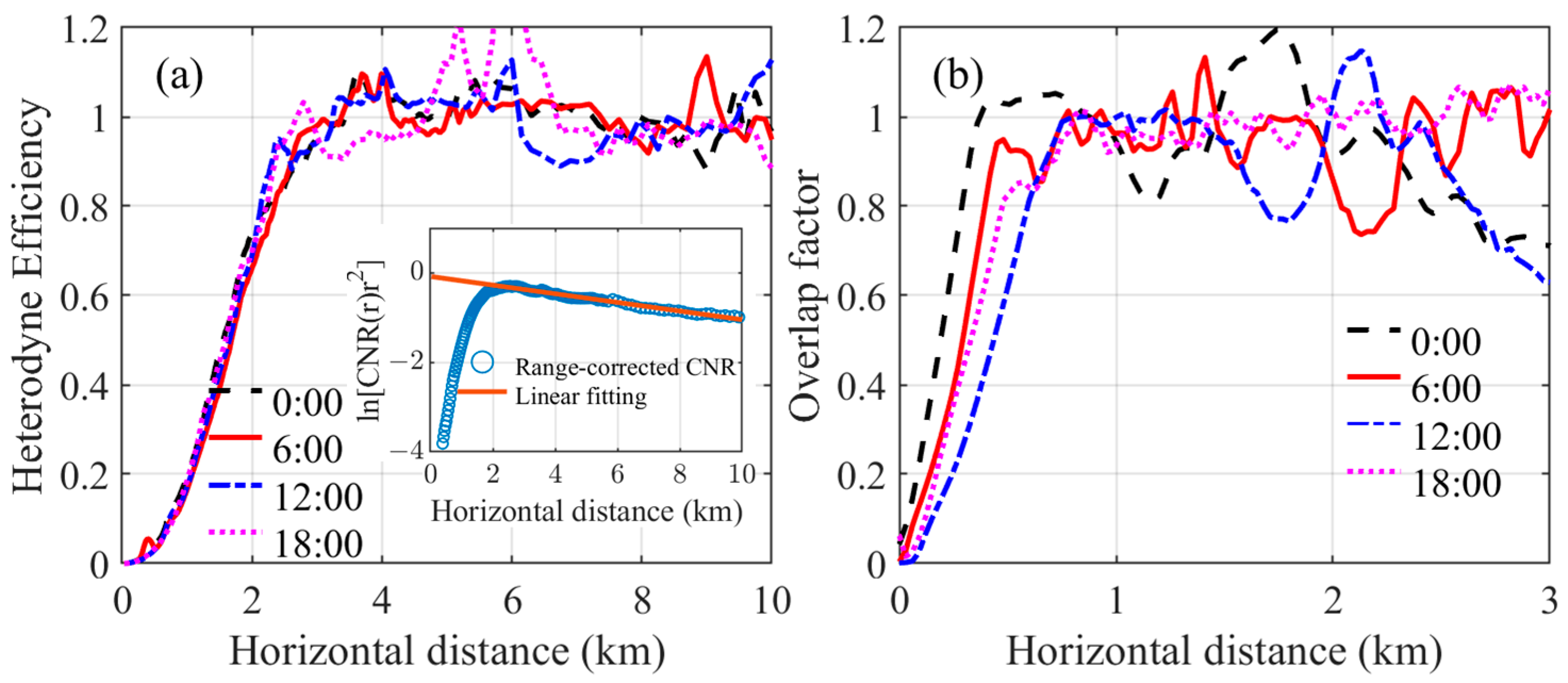
Similar to the processing method of overlap factor correction [37], the modulation of the heterodyne efficiency over the backscatter signal can be estimated from the horizontal measurements. To calibrate the heterodyne efficiency in the near field, an advanced horizontal measurement is performed, and the average result of the CNR is applied and fitted, as shown in the subfigure of Figure 1a. Due to the different range resolutions, the density of numerical points varies with the range. Using the ratio of the range-correct CNR and the linear fit result, the heterodyne efficiency can be obtained and used to calibrate the CNR profiles in the experiment. Figure 1a depicts four heterodyne efficiency profiles at different times, which seem to be stable within the range of 3 km due to the all-fiber structure and the stable temperature of the system.
In contrast, limited by the non-coaxial telescope and the space optical structure, the RMRL system is more affected by temperature changes, which are huge in the desert. Figure 1b depicts four overlap factor profiles of the 355 nm channel, measured at 0:00, 6:00, 12:00, and 18:00 local time on 14 February 2023. The temperature variation affects the optical coupling of the space optical system significantly, resulting in an unstable overlap factor for the RMRL. The signal in the near field, mainly below 0.5 km is distorted, so only the results above 0.5 km are involved in the comparison.
As mentioned earlier, the CDWL is operated in a VAD scanning mode with an elevation angle of 70°. The CNR profiles have to be converted vertically to match the backscatter profiles of the RMRL, so an approximation is taken so that the average CNR of a circle scan is approximate to the vertical CNR profile at the projection height. Furthermore, the vertical CNR profile is interpolated to a height resolution of 30 m to match the profile of the RMRL.
3.2. Retrieval of the RMRL
In this subsection, two methods are used to retrieve the optical properties of aerosols. Generally, by assuming a constant lidar ratio between and , the inversion algorithm proposed by Klett and Fernald (KF method) can be used to retrieve and [38,39]. This method can be used to invert the extinction and backscatter with only one elastic backscatter lidar, with the assumption of the lidar ratio and boundary value. Different assumptions of boundary value may lead to various results [40,41]. In general, the boundary value is chosen at a reference altitude where the atmosphere is relatively pure and the signal-to-noise ratio (SNR) is high enough. Sometimes, it may be difficult to find the reference height, and soft targets such as clouds are used to estimate the boundary value [42].
In addition, the Raman backscatter signals can be used alone to retrieve aerosol extinction profiles [43]. The independent aerosol extinction coefficient can be expressed as: [44,45]
where the subscripts and stand for aerosol and atmospheric molecules, respectively. is the number density of the Raman molecule; and are the wavelength of the Raman-shifted laser and the output laser, respectively. is the backscatter power of the Raman-shifted signal, and is the Angstrom exponent. With the combination of Mie scattering data, aerosol backscatter coefficient profiles can be obtained by:
where is the reference height and is the backscatter power of the Mie lidar signal. can be calculated by the atmospheric temperature and pressure from the radiosonde measurement or the atmosphere model. The two approaches present different advantages and disadvantages; for example, the KF method relies on the accurate assumption of the lidar ratio and boundary value, and the Raman method relies on the accurate assumption of the Angstrom exponent. Figure 2 depicts some retrieval results of the experiments, and the two algorithms show good consistency under correct assumptions.
To compare the data retrieval of the RMRL and CDWL, the backscatter and extinction coefficients of aerosol at the wavelengths of 355, 532, and 1064 nm had to be converted to the wavelength of 1548 nm. However, the extinction coefficient retrieved with the Raman method only uses the backscatter signal at the Raman wavelength of 386 nm, which may bring errors to the data conversion process. In this work, the two methods were combined. First, the aerosol extinction coefficient was obtained at the reference height with the Raman method using the data from 386 nm and then applied to the KF method as the boundary value. Next, with the KF method, the extinction coefficient at the wavelengths of 355, 532, and 1064 nm could be obtained using the data from the different elastic lidars. The Angstrom exponent varies with the wavelength, and an empirical relationship between aerosol extinction and wavelength can be expressed with a second-order polynomial [46,47]:
where the coefficient accounts for a “curvature” often observed in Sun photometry measurements. For a special case of , Equation (6) equals the Angstrom exponent law and . With the profiles of the aerosol extinction coefficient from the RMRL, the profiles of the aerosol extinction and the backscatter coefficient at the wavelength of 1548 nm can be obtained, as shown in Figure 3.
In this way, the data sets of the two lidars were assimilated to the same wavelength and their inversion results could be compared. The data processing procedure is displayed in Figure 4. The number density of Nitrogen molecules was calculated by the profile of temperature and pressure from the Atmosphere model, and the lidar ratio was set as 30/32/45/50 Sr at the wavelength of 355/532/1064/1548 nm.
4. Experiments and Results
Field joint experiments with the CDWL and RMRL were conducted from 16 to 21 February 2023. The Raman lidar only works from 22:00 to 6:00 local time, so only the data during the nighttime were compared. Figure 5 depicts the backscatter profiles averaged over ten minutes altitude during the nighttime and daytime. Both the CDWL and RMRL demonstrate a vertical detection capability of more than 3 km during the nighttime, and it can be seen that the aerosols are mainly distributed at altitudes below 3 km. The backscatter signal at 386 nm decays smoothly because the Raman backscatter coefficient is proportional to the density of nitrogen, which is independent of the aerosol profiles. During the daytime, the Raman lidar is turned off, and the effective detection ranges of the other lidars are also reduced.
With the method in Figure 4, the extinction coefficients at various wavelengths were retrieved with the resolution of 30 m/1 min, as shown in Figure 6, which also can be used to retrieve the color ratio. Only the results from 22:00 to 6:00 local time are plotted. Figure 6d, e shows the extinction coefficients at 1548 nm using the data from the RMRL and CDWL, respectively, and the comparison results show good consistency.
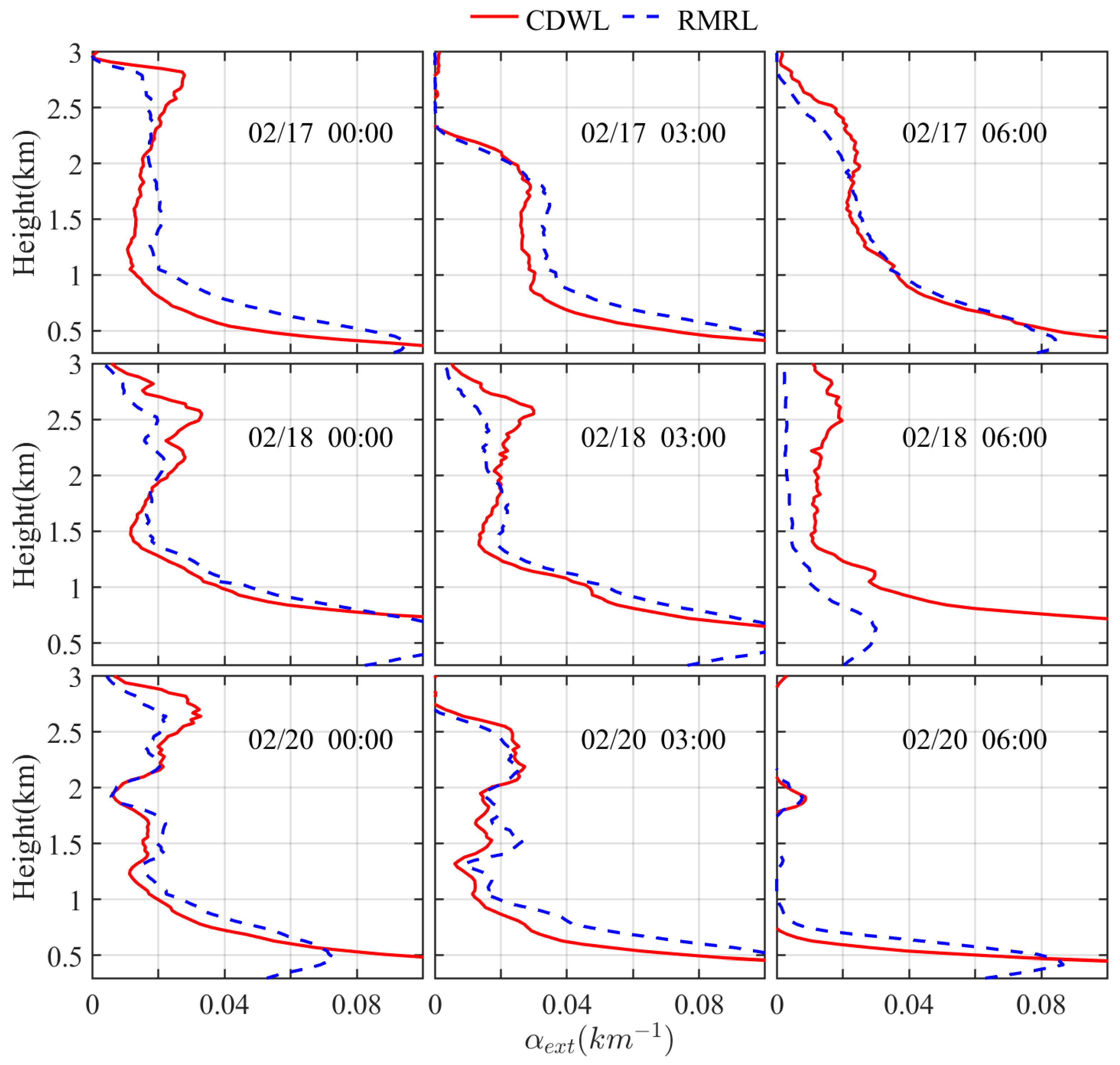
It can be noticed that longitudinal stripes appear in Figure 6, which may mean the internal gravity waves strongly affect the backscatter, particularly at 0:00 on 20 February. To compare the retrieval of extinction coefficients with the two lidars in detail, the results within a height range at the same time are displayed, as shown in Figure 7. It needs to be mentioned that the results vary greatly in the near field (mainly in altitudes ranging below 0.5 km). The signal of the RMRL is uncalibrated in the range of 0–0.5 km due to the lack of a stable overlap factor, while the CDWL is calibrated with a relatively stable heterodyne efficiency. Inconsistent results appear at 6:00 local time on 18 February, the output power of the laser in the RMRL decreases, and the effective detection distance is reduced. Consequently, the measurement of the RMRL shows poor ability in aerosol retrieval, causing a large difference between the CDWL and RMRL.
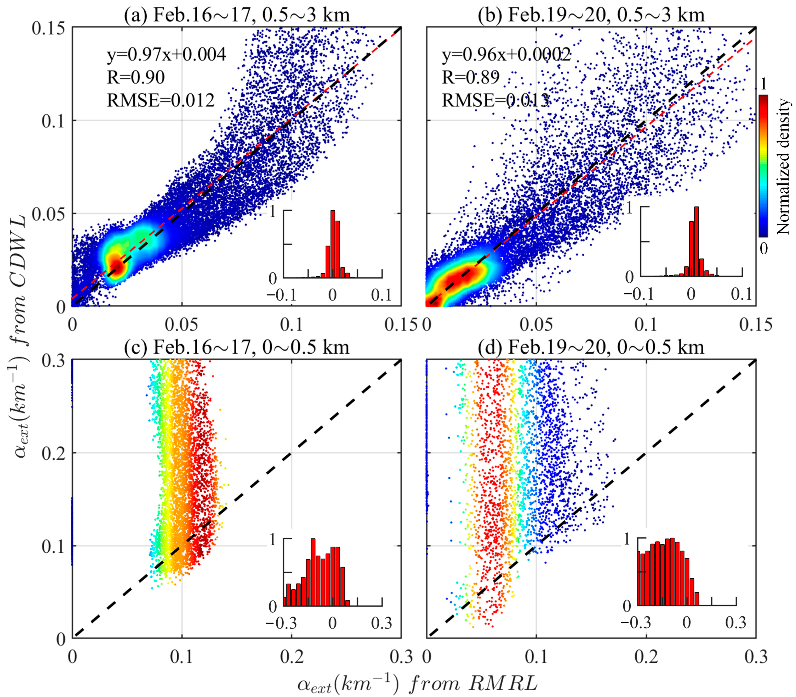
The scatter diagrams of the aerosol extinction coefficients retrieved from the CDWL and RMRL are shown in Figure 8. The results of the CDWL are plotted versus those of the RMRL, and the density of the data points is normalized and displayed in different colors. Moreover, the distributions of the bias are inserted in the bottom right corner of each panel, in which the negative bias means that the results of the CDWL are lower than that of the RMRL. In addition, due to the effects of different overlap factors, comparisons using data ranging from 0.5 to 3 km and from 0 to 0.5 km are divided into two groups. The first-order linear fitting functions of the results, the determination coefficients R, and the root-mean-square error (RMSE) are added to the upper left corner of each graph. Good performance with an R of 0.90 and 0.89 was obtained, proving the accuracy of aerosol retrieval by coherent detection after heterodyne efficiency correction. In contrast, results ranging from 0 to 0.5 km are shown in Figure 8c,d. The uncorrected overlap factor leads to the result that the aerosol extinction of the RMRL is smaller than that of the CDWL.
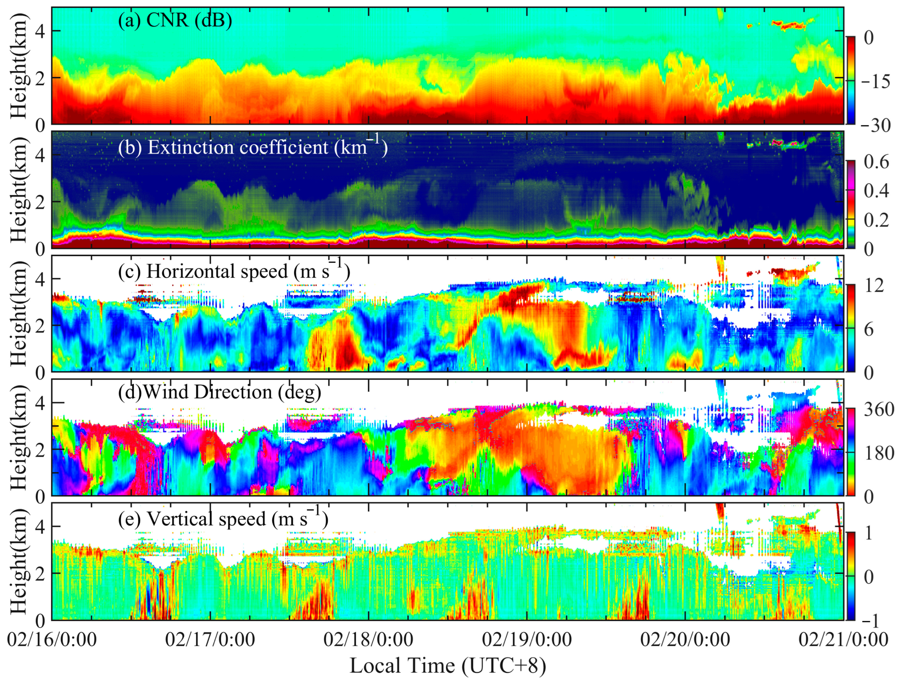
The continuous observation results from 16–21 February are shown in Figure 9, including the CNR, aerosol extinction coefficients, horizontal wind speed and direction, and vertical wind speed. When the Raman lidar does not work during the daytime, the boundary value is set as the interpolation of the result during the night. To ensure the accuracy of the results, the retrieval of wind speed and direction with the CNR less than −17 dB is plotted as white. In Figure 9e, the positive value of vertical velocity is defined as downward, and the upward wind speed appearing every afternoon is consistent with the results of the extinction coefficient, which also confirms the vertical transport process of aerosols. The results prove the aerosol retrieval capability of the CDWL system.
5. Conclusions
An experimental comparison between aerosol measurements using the CDWL and the RMRL was achieved. To calibrate the aerosol retrieval, a method using boundary values from the Raman lidar was proposed, and the extinction coefficients were compared from the two lidar systems. Good agreements were achieved during the continuous field experiments, with the fitting slopes of 0.97 and 0.96, and the determination coefficients of 0.90 and 0.89. The results prove the accuracy of aerosol retrieval by coherent lidar after correction powerfully, and the aerosol detection by all-fiber wind lidar was extended, which may achieve the miniaturization and stabilization of the lidar for meteorological measurements.
Author Contributions
Conceptualization, M.L. and H.X.; methodology, M.L.; formal analysis, H.X. and M.L.; investigation, M.L.; data curation, L.S. and X.W.; writing—original draft preparation, M.L.; writing—review and editing, M.L., L.S., X.W., J.Y., H.H. and H.X.; visualization, M.L.; supervision, H.X. and H.H. All authors have read and agreed to the published version of the manuscript.
Funding
Strategic Priority Research Program of Chinese Academy of Sciences, grant number XDA22040601.
Data Availability Statement
The data underlying the results presented in this paper can be obtained from the authors upon reasonable request.
Acknowledgments
We would like to thank the Xinjiang Uygur Autonomous Region Meteorological Service for providing support with the observational data.
Conflicts of Interest
The authors declare no conflict of interest.
References
- Kokhanovsky, A.A. Aerosol Optics: Light Absorption and Scattering by Particles in the Atmosphere; Springer Science & Business Media: Berlin, Germany, 2008. [Google Scholar]
- Stocker, T. Climate Change 2013: The Physical Science Basis: Working Group I Contribution to the Fifth Assessment Report of the Intergovernmental Panel on Climate Change; Cambridge University Press: Cambridge, UK, 2014. [Google Scholar]
- Caicedo, V.; Rappenglück, B.; Lefer, B.; Morris, G.; Toledo, D.; Delgado, R. Comparison of aerosol lidar retrieval methods for boundary layer height detection using ceilometer aerosol backscatter data. Atmos. Meas. Tech. 2017, 10, 1609–1622. [Google Scholar] [CrossRef]
- Gryazin, V.; Beresnev, S. Influence of vertical wind on stratospheric aerosol transport. Meteorol. Atmos. Phys. 2011, 110, 151–162. [Google Scholar] [CrossRef]
- Yuan, J.; Wu, Y.; Shu, Z.; Su, L.; Tang, D.; Yang, Y.; Dong, J.; Yu, S.; Zhang, Z.; Xia, H. Real-Time Synchronous 3-D Detection of Air Pollution and Wind Using a Solo Coherent Doppler Wind Lidar. Remote Sens. 2022, 14, 2809. [Google Scholar] [CrossRef]
- Petit, J.-E.; Favez, O.; Albinet, A.; Canonaco, F. A user-friendly tool for comprehensive evaluation of the geographical origins of atmospheric pollution: Wind and trajectory analyses. Environ. Model. Softw. 2017, 88, 183–187. [Google Scholar] [CrossRef]
- Menzies, R.T.; Tratt, D.M. Airborne CO2 coherent lidar for measurements of atmospheric aerosol and cloud backscatter. Appl. Opt. 1994, 33, 5698–5711. [Google Scholar] [CrossRef]
- Winker, D.M.; Vaughan, M.A.; Omar, A.; Hu, Y.; Powell, K.A.; Liu, Z.; Hunt, W.H.; Young, S.A. Overview of the CALIPSO mission and CALIOP data processing algorithms. J. Atmos. Oceanic Technol. 2009, 26, 2310–2323. [Google Scholar] [CrossRef]
- Shimizu, A.; Nishizawa, T.; Jin, Y.; Kim, S.-W.; Wang, Z.; Batdorj, D.; Sugimoto, N. Evolution of a lidar network for tropospheric aerosol detection in East Asia. Opt. Eng. 2017, 56, 031219. [Google Scholar] [CrossRef]
- Zhao, C.; Wang, Y.; Wang, Q.; Li, Z.; Wang, Z.; Liu, D. A new cloud and aerosol layer detection method based on micropulse lidar measurements. J. Geophys. Res. Atmos. 2014, 119, 6788–6802. [Google Scholar] [CrossRef]
- Li, M.; Wu, Y.; Yuan, J.; Zhao, L.; Tang, D.; Dong, J.; Xia, H.; Dou, X. Stratospheric aerosol lidar with a 300 µm diameter superconducting nanowire single-photon detector at 1064 nm. Opt. Express 2023, 31, 2768–2779. [Google Scholar] [CrossRef]
- Dang, R.; Yang, Y.; Hu, X.-M.; Wang, Z.; Zhang, S. A review of techniques for diagnosing the atmospheric boundary layer height (ABLH) using aerosol lidar data. Remote Sens. 2019, 11, 1590. [Google Scholar] [CrossRef]
- Engelmann, R.; Wandinger, U.; Ansmann, A.; Müller, D.; Žeromskis, E.; Althausen, D.; Wehner, B. Lidar observations of the vertical aerosol flux in the planetary boundary layer. J. Atmos. Oceanic Technol. 2008, 25, 1296–1306. [Google Scholar] [CrossRef]
- Arshinov, Y.F.; Bobrovnikov, S.M.; Zuev, V.E.; Mitev, V. Atmospheric temperature measurements using a pure rotational Raman lidar. Appl. Opt. 1983, 22, 2984–2990. [Google Scholar] [CrossRef] [PubMed]
- Hua, D.; Uchida, M.; Kobayashi, T. Ultraviolet high-spectral-resolution Rayleigh–Mie lidar with a dual-pass Fabry–Perot etalon for measuring atmospheric temperature profiles of the troposphere. Opt. Lett. 2004, 29, 1063–1065. [Google Scholar] [CrossRef] [PubMed]
- Yu, S.; Zhang, Z.; Xia, H.; Dou, X.; Wu, T.; Hu, Y.; Li, M.; Shangguan, M.; Wei, T.; Zhao, L. Photon-counting distributed free-space spectroscopy. Light Sci. Appl. 2021, 10, 212. [Google Scholar] [CrossRef] [PubMed]
- Abshire, J.B.; Ramanathan, A.; Riris, H.; Mao, J.; Allan, G.R.; Hasselbrack, W.E.; Weaver, C.J.; Browell, E.V. Airborne measurements of CO2 column concentration and range using a pulsed direct-detection IPDA lidar. Remote Sens. 2013, 6, 443–469. [Google Scholar] [CrossRef]
- Xia, H.; Dou, X.; Sun, D.; Shu, Z.; Xue, X.; Han, Y.; Hu, D.; Han, Y.; Cheng, T. Mid-altitude wind measurements with mobile Rayleigh Doppler lidar incorporating system-level optical frequency control method. Opt. Express 2012, 20, 15286–15300. [Google Scholar] [CrossRef]
- Tucker, S.C.; Senff, C.J.; Weickmann, A.M.; Brewer, W.A.; Banta, R.M.; Sandberg, S.P.; Law, D.C.; Hardesty, R.M. Doppler lidar estimation of mixing height using turbulence, shear, and aerosol profiles. J. Atmos. Oceanic Technol. 2009, 26, 673–688. [Google Scholar] [CrossRef]
- Wang, L.; Qiang, W.; Xia, H.; Wei, T.; Yuan, J.; Jiang, P. Robust solution for boundary layer height detections with coherent doppler wind lidar. Adv. Atmos. Sci. 2021, 38, 1920–1928. [Google Scholar] [CrossRef]
- Yuan, J.; Xia, H.; Wei, T.; Wang, L.; Yue, B.; Wu, Y. Identifying cloud, precipitation, windshear, and turbulence by deep analysis of the power spectrum of coherent Doppler wind lidar. Opt. Express 2020, 28, 37406–37418. [Google Scholar] [CrossRef]
- Smalikho, I.N.; Banakh, V.; Holzäpfel, F.; Rahm, S. Method of radial velocities for the estimation of aircraft wake vortex parameters from data measured by coherent Doppler lidar. Opt. Express 2015, 23, A1194–A1207. [Google Scholar] [CrossRef]
- Wei, T.; Xia, H.; Hu, J.; Wang, C.; Shangguan, M.; Wang, L.; Jia, M.; Dou, X. Simultaneous wind and rainfall detection by power spectrum analysis using a VAD scanning coherent Doppler lidar. Opt. Express 2019, 27, 31235–31245. [Google Scholar] [CrossRef]
- Tridon, F.; Battaglia, A. Dual-frequency radar Doppler spectral retrieval of rain drop size distributions and entangled dynamics variables. J. Geophys. Res. Atmos. 2015, 120, 5585–5601. [Google Scholar] [CrossRef]
- Abdelazim, S.; Santoro, D.; Arend, M.F.; Moshary, F.; Ahmed, S. Development and operational analysis of an all-fiber coherent Doppler lidar system for wind sensing and aerosol profiling. IEEE Trans. Geosci. Remote Sens. 2015, 53, 6495–6506. [Google Scholar] [CrossRef]
- Belmonte, A. Analyzing the efficiency of a practical heterodyne lidar in the turbulent atmosphere: Telescope parameters. Opt. Express 2003, 11, 2041–2046. [Google Scholar] [CrossRef]
- Chouza, F.; Reitebuch, O.; Groß, S.; Rahm, S.; Freudenthaler, V.; Toledano, C.; Weinzierl, B. Retrieval of aerosol backscatter and extinction from airborne coherent Doppler wind lidar measurements. Atmos. Meas. Tech. 2015, 8, 2909–2926. [Google Scholar] [CrossRef]
- Dai, G.; Wang, X.; Sun, K.; Wu, S.; Song, X.; Li, R.; Yin, J.; Wang, X. Calibration and retrieval of aerosol optical properties measured with Coherent Doppler Lidar. J. Atmos. Oceanic Technol. 2021, 38, 1035–1045. [Google Scholar] [CrossRef]
- Yang, S.; Preißler, J.; Wiegner, M.; von Löwis, S.; Petersen, G.N.; Parks, M.M.; Finger, D.C. Monitoring Dust Events Using Doppler Lidar and Ceilometer in Iceland. Atmosphere 2020, 11, 1294. [Google Scholar] [CrossRef]
- Zhang, Y.; Zheng, Y.; Tan, W.; Guo, P.; Xu, Q.; Chen, S.; Lin, R.; Chen, S.; Chen, H. Two Practical Methods to Retrieve Aerosol Optical Properties from Coherent Doppler Lidar. Remote Sens. 2022, 14, 2700. [Google Scholar] [CrossRef]
- O’Connor, E.J.; Illingworth, A.J.; Hogan, R.J. A technique for autocalibration of cloud lidar. J. Atmos. Oceanic Technol. 2004, 21, 777–786. [Google Scholar] [CrossRef]
- Huang, T.; Yang, Y.; O’Connor, E.J.; Lolli, S.; Haywood, J.; Osborne, M.; Cheng, J.C.; Guo, J.; Yim, S.H. Influence of a weak typhoon on the vertical distribution of air pollution in Hong Kong: A perspective from a Doppler LiDAR network. Environ. Pollut. 2021, 276, 116534. [Google Scholar] [CrossRef]
- Pentikäinen, P.; O’Connor, E.J.; Manninen, A.J.; Ortiz-Amezcua, P. Methodology for deriving the telescope focus function and its uncertainty for a heterodyne pulsed Doppler lidar. Atmos. Meas. Tech. 2020, 13, 2849–2863. [Google Scholar] [CrossRef]
- Newsom, R.K.; Brewer, W.A.; Wilczak, J.M.; Wolfe, D.E.; Oncley, S.P.; Lundquist, J.K. Validating precision estimates in horizontal wind measurements from a Doppler lidar. Atmos. Meas. Tech. 2017, 10, 1229–1240. [Google Scholar] [CrossRef]
- Henderson, S.W.; Gatt, P.; Rees, D.; Huffaker, R.M. Wind lidar. In Laser Remote Sensing; CRC Press: Boca Raton, FL, USA, 2005; pp. 487–740. [Google Scholar]
- Fujii, T.; Fukuchi, T. Laser Remote Sensing; CRC Press: Boca Raton, FL, USA, 2005. [Google Scholar]
- Berkoff, T.A.; Welton, E.J.; Campbell, J.R.; Scott, V.; Spinhirne, J.D. Investigation of overlap correction techniques for the Micro-Pulse Lidar NETwork (MPLNET). In Proceedings of the IGARSS 2003, IEEE International Geoscience and Remote Sensing Symposium, Toulouse, France, 21–25 July 2003; pp. 4395–4397. [Google Scholar]
- Fernald, F.G. Analysis of atmospheric lidar observations: Some comments. Appl. Opt. 1984, 23, 652–653. [Google Scholar] [CrossRef]
- Klett, J.D. Lidar inversion with variable backscatter/extinction ratios. Appl. Opt. 1985, 24, 1638–1643. [Google Scholar] [CrossRef] [PubMed]
- Matsumoto, M.; Takeuchi, N. Effects of misestimated far-end boundary values on two common lidar inversion solutions. Appl. Opt. 1994, 33, 6451–6456. [Google Scholar] [CrossRef] [PubMed]
- Jinhuan, Q. Sensitivity of lidar equation solution to boundary values and determination of the values. Adv. Atmos. Sci. 1988, 5, 229–241. [Google Scholar] [CrossRef]
- Ershov, A.D.; Balin, Y.S.; Samoilova, S.V. Inversion of the lidar data in investigations of the optical characteristics of weakly turbid atmosphere. In Ninth Joint International Symposium on Atmospheric and Ocean Optics/Atmospheric Physics. Part II: Laser Sensing and Atmospheric Physics; SPIE: Bellingham, WA, USA, 2003; pp. 168–171. [Google Scholar] [CrossRef]
- Gong, W.; Zhang, J.; Mao, F.; Li, J. Measurements for profiles of aerosol extinction coeffcient, backscatter coeffcient, and lidar ratio over Wuhan in China with Raman/Mie lidar. Chin. Opt. Lett. 2010, 8, 533–536. [Google Scholar] [CrossRef]
- Melfi, S. Remote measurements of the atmosphere using Raman scattering. Appl. Opt. 1972, 11, 1605–1610. [Google Scholar] [CrossRef]
- Whiteman, D.; Melfi, S.; Ferrare, R. Raman lidar system for the measurement of water vapor and aerosols in the Earth’s atmosphere. Appl. Opt. 1992, 31, 3068–3082. [Google Scholar] [CrossRef]
- Schuster, G.L.; Dubovik, O.; Holben, B.N. Angstrom exponent and bimodal aerosol size distributions. J. Geophys. Res. Atmos. 2006, 111, D07207. [Google Scholar] [CrossRef]
- O’Neill, N.; Eck, T.; Holben, B.; Smirnov, A.; Dubovik, O.; Royer, A. Bimodal size distribution influences on the variation of Angstrom derivatives in spectral and optical depth space. J. Geophys. Res. Atmos. 2001, 106, 9787–9806. [Google Scholar] [CrossRef]
Figure 1.
(a) The heterodyne efficiency from four horizontal experiments, which was obtained from the ratio of the range−correct CNR (blue circles) and the linear fit result (orange line), as shown in the subfigure. (b) The overlap factor of the 355 nm channel from three horizontal experiments, measured at 0:00, 6:00, 12:00, and 18:00 local time on 14 February 2023.

Figure 2.
Comparison of retrieval using the Raman method (blue dotted line) and the KF method (red line). Aerosol backscatter coefficient from the data of (a) 355 nm, (b) 532 nm, and (c) 1064 nm lidar observed at 1:30 local time on 20 February 2023. The lidar ratios assumed for KF inversion are 30, 32, and 45. The Angstrom exponent applied in Equation (4) is set as 1.5.

Figure 3.
(a) Three groups of aerosol extinction coefficients at a height of 2 km retrieved from the RMRL (red dots); second-order poly fit curves using the extinction coefficients and the wavelength (blue line); aerosol extinction coefficients at the wavelength of 1548 nm derived from the poly fit curves (blue triangle); (b) a magnification of part of (a) from 1.5 to 1.6 μm; aerosol extinction coefficients retrieved from the CDWL (pink square), and the blue lines and blue triangles are the same as in (a), derived from the RMRL. The gray circles indicate the same group of data.

Figure 4.
Overview of the data processing procedure. CDWL, coherent Doppler wind lidar; DC, direct current.
Figure 4.
Overview of the data processing procedure. CDWL, coherent Doppler wind lidar; DC, direct current.

Figure 5.
Ten minutes averaged altitude profiles of backscattered signals measured at (a) 0:00 and (b) 12:00 local time on 20 February. The Raman lidar does not work during the daytime. The legend indicates the wavelengths of the backscatter signals in nanometers.
Figure 5.
Ten minutes averaged altitude profiles of backscattered signals measured at (a) 0:00 and (b) 12:00 local time on 20 February. The Raman lidar does not work during the daytime. The legend indicates the wavelengths of the backscatter signals in nanometers.

Figure 6.
Results of extinction coefficients at the wavelengths of (a) 355 nm; (b) 532 nm; (c) 1064 nm; (d) 1548 nm using the RMRL; (e) and 1548 nm using the CDWL. The results from 22:00 to 6:00 local time on the 16, 17, 18, 19, and 20 February are displayed when the Raman lidar works routinely. The time resolution and height resolution are 1 min and 30 m, respectively.

Figure 7.
Comparison of the aerosol extinction coefficients with the two lidars, measured at 0:00, 3:00, and 6:00 local time on the 17, 18, and 20 February, respectively. The red lines show the results of the CDWL at 1548 nm, and the blue dotted lines show the fitting results of the RMRL at 1548 nm.

Figure 8.
Scatter diagrams of the aerosol extinction coefficients derived from the RMRL and the CDWL. Results ranging from 0.5 to 3 km during the nighttime of the 17 and 20 February are compared in Figure 8 (a,b), respectively. In contrast, results ranging from 0 to 0.5 km are shown in Figure 8 (c,d). The color-shaded dots denote the normalized density. The black dashed lines denote 1:1 lines, and the red dashed lines show the linear fitting results. The distributions of y-x are inserted in the bottom right corner of each panel.

Figure 9.
Continuous observation by the CDWL from the 16 to 21 February. (a) CNR, (b) aerosol extinction coefficient, (c) horizontal wind speed, (d) horizontal wind direction, and (e) vertical wind speed. The CNR and extinction coefficient are averaged over a vertical scanning duration of 1 min. The positive value of vertical velocity is defined as downward.


Table 1.
Key parameters of CDWL and RMRL systems.
| Parameter | CDWL | RMRL | |
|---|---|---|---|
| Laser | |||
| Wavelength | 1548 nm | 355/532/1064 nm | |
| Frequency offset | 80 MHz | / | |
| Pulse energy | 110 μJ | 250/350/350 mJ | |
| Repetition rate | 10 kHz | 20 Hz | |
| Pulse width | 200 ns | 8 ns | |
| Telescope | |||
| Diameter | 100 mm | 450 mm | |
| Elevation angle | 70° | 90° | |
| Data acquisition | Detection type | BD | PMT |
| Noise bandwidth | 200 MHz | 0.3 nm | |
| Sampling rate | 250 MHz | 20 MHz | |
| Temporal resolution | 1 s | 60 s | |
| Spatial resolution | 30, 60, 150 m | 30 m |
Disclaimer/Publisher’s Note: The statements, opinions and data contained in all publications are solely those of the individual author(s) and contributor(s) and not of MDPI and/or the editor(s). MDPI and/or the editor(s) disclaim responsibility for any injury to people or property resulting from any ideas, methods, instructions or products referred to in the content. |
© 2023 by the authors. Licensee MDPI, Basel, Switzerland. This article is an open access article distributed under the terms and conditions of the Creative Commons Attribution (CC BY) license (https://creativecommons.org/licenses/by/4.0/).
Share and Cite
MDPI and ACS Style
Li, M.; Xia, H.; Su, L.; Han, H.; Wang, X.; Yuan, J. The Detection of Desert Aerosol Incorporating Coherent Doppler Wind Lidar and Rayleigh–Mie–Raman Lidar. Remote Sens. 2023, 15, 5453. https://doi.org/10.3390/rs15235453
AMA Style
Li M, Xia H, Su L, Han H, Wang X, Yuan J. The Detection of Desert Aerosol Incorporating Coherent Doppler Wind Lidar and Rayleigh–Mie–Raman Lidar. Remote Sensing. 2023; 15(23):5453. https://doi.org/10.3390/rs15235453
Chicago/Turabian StyleLi, Manyi, Haiyun Xia, Lian Su, Haobin Han, Xiaofei Wang, and Jinlong Yuan. 2023. "The Detection of Desert Aerosol Incorporating Coherent Doppler Wind Lidar and Rayleigh–Mie–Raman Lidar" Remote Sensing 15, no. 23: 5453. https://doi.org/10.3390/rs15235453
Note that from the first issue of 2016, this journal uses article numbers instead of page numbers. See further details here.