Article

Modeling of Suspended Particulate Matter Concentration in an Extremely Turbid River Based on Multispectral Remote Sensing from an Unmanned Aerial Vehicle (UAV)

1
College of Urban and Environmental Sciences, Northwest University, Xi’an 710127, China
2
Shaanxi Key Laboratory of Earth Surface System and Environmental Carrying Capacity, Xi’an 710127, China
3
Key Laboratory of Watershed Geographic Sciences, Nanjing Institute of Geography and Limnology, Chinese Academy of Sciences, Nanjing 210008, China
4
Analytical Applications Center, Shimadzu (China) Co., Ltd., Xi’an 710127, China
*
Author to whom correspondence should be addressed.
Remote Sens. 2023, 15(22), 5398; https://doi.org/10.3390/rs15225398
Submission received: 7 October 2023 / Revised: 14 November 2023 / Accepted: 15 November 2023 / Published: 17 November 2023

Abstract

:
Following consecutive years of governance efforts, there has been a substantial reduction in sediment transport in the Yellow River, resulting in significant changes in its water–sediment dynamics. This necessitates precise monitoring of sediment-bearing tributary inflows, a crucial requirement for effective governance strategies on the Loess Plateau’s current developmental stage. While satellite remote sensing technology has been widely used to estimate suspended particulate matter concentration (CSPM) in open water bodies like oceans and lakes, its application in narrow rivers presents challenges related to hybrid pixel and proximity effects. As a result, the effectiveness and competence of satellite remote sensing in monitoring CSPM in such confined river environments are reduced. This study attempted to use unmanned aerial vehicle (UAV) remote sensing with multispectral technology to invert CSPM in the Wuding River, a sediment-bearing Yellow River tributary. A novel CSPM concentration inversion model was introduced for highly turbid river settings. The results showed that the accuracy of the new band ratio model in this study is significantly improved compared with the existing models. The validation dataset had a coefficient of determination (R2) of 0.83, a root mean square error (RMSE) of 3.73 g/L, and a mean absolute percentage error (MAPE) of 44.95% (MAPE is 40.68% at 1–20 g/L, and 12.37% at >20 g/L). On this basis, the UAV also monitored the impacts of heavy rainfall on the CSPM, resulting in a rapid rise and fall in CSPM over a period of ten hours. This study demonstrated the potential of UAV remote sensing for CSPM monitoring in extremely turbid narrow rivers (tens to tens of meters), especially before and after rainfall sediment production events, which can provide technical support for accurate sediment management and source identification in the main tributaries of the Yellow River and help realize the goal of high-quality development of the Yellow River Basin.

Graphical Abstract

1. Introduction

The Yellow River is a prototypical sediment-bearing river on a global scale, characterized by a paucity of water relative to sediment. Its distribution of water and sediment exhibits a pronounced imbalance. In the middle reaches, the Loess Plateau grapples with severe soil erosion, leading to a substantial inflow of sediment into the primary channel of the Yellow River via its tributaries [1]. As a consequence, there is a discernible escalation in sediment content in both the middle and lower reaches of the main stem. This phenomenon not only complicates the effective utilization of water resources in the middle reaches but also causes an elevation of the riverbed in the lower reaches, culminating in the formation of a ‘secondary overhanging river’ [2]. Such a situation poses a substantial threat to both lives and property. Consequently, the issue of sediment management in the Yellow River has emerged as a pivotal and highly relevant research focus.
Traditional river sediment monitoring predominantly relies on station observations and field sampling and measurements. In the middle reaches of the Yellow River, there are more than 500 hydrological stations at various levels capable of providing accurate sediment content data at a daily scale. Nonetheless, these hydrological stations demand high operational and maintenance costs. Furthermore, taking field measurements is a time-consuming and labor-intensive process, and the data acquired from these stations are limited to specific points, failing to precisely represent the spatial dynamics of river sediment.
After decades of long-term management of the Yellow River, sediment transport in the main stream has significantly decreased. This reduction in sediment transport has transitioned into a new phase of precision management, necessitating ongoing spatial monitoring of the primary sediment tributaries to accurately pinpoint sediment sources. Suspended Particulate Matter (SPM) concentration, denoted as CSPM, serves as a key indicator of suspended sediment content, concluding clay and silt particles with a diameter of less than 2 mm [3]. SPM induces noticeable alterations in optical signals at specific wavelengths on the water surface, rendering satellite remote sensing a successful method for monitoring CSPM dynamics in various open water bodies, such as oceans, lakes, and reservoirs [4,5].
Nevertheless, the Yellow River tributaries exhibit distinct characteristics; they tend to be narrower and longer than the main channel, typically spanning only tens of meters in width. Satellite sensors, constrained by their spatial resolution, often encounter challenges in accurately capturing data in these tributaries. This limitation results in mixed pixels at the boundary between land and water bodies, and the interference caused by adjacent pixel effects becomes conspicuous. Furthermore, short-term heavy rainfall stands as one of the primary contributors to sediment production in the middle reaches of the Yellow River [6]. However, satellites frequently face difficulties in acquiring effective data due to the influence of adverse weather conditions. The rapid advancements in UAV remote sensing technology present a promising solution to these issues. UAVs offer distinct advantages, including high spatial resolution, reduced susceptibility to weather and atmospheric interference, and the flexibility to acquire remote sensing images as needed. Consequently, UAV-based remote sensing holds considerable potential for effectively monitoring CSPM in the primary sediment-bearing tributaries of the Yellow River [7,8].
Given the substantial impact of CSPM on the spectral signals of water bodies, researchers both domestically and internationally have proposed several well-established inversion methods, encompassing empirical, semi-empirical, and semi-analytical models as summarized in Table 1. Empirical and semi-empirical models operate by deriving CSPM concentrations through the selection of optimal spectral bands or band combinations using specific mathematical techniques. These models establish empirical–statistical relationships directly between remotely sensed data and measured CSPM values [9]. Previous research has demonstrated that single-band models can yield satisfactory results when characteristic bands of the spectral curve are distinct [10,11]. Alternatively, some researchers have employed the band ratio method to select the input parameter that exhibits the highest correlation with CSPM among all possible band combinations [12]. Semi-analytical methods, on the other hand, are rooted in modeling the varying absorption and scattering characteristics of water bodies. For instance, Jiang [13] categorized water bodies into four types—clear, moderately turbid, highly turbid, and extremely turbid—by comparing remote sensing reflectance (Rrs) at wavelengths 490, 560, 620, and 754 nm. Leveraging the distinct relationships between CSPM and backward scattering coefficients (bbp) in each type, a semi-analytical approach was employed to formulate unique inversion models for each water body category. However, it is noteworthy that the CSPM concentrations in the existing models generally span from tens to thousands of mg/L. In contrast, the Yellow River and its major sediment-bearing tributaries can experience concentrations in the tens of thousands of mg/L in a short timeframe following heavy rainfall events. Consequently, there exists uncertainty regarding the applicability of current inversion models to the exceptionally turbid river conditions encountered in this study.
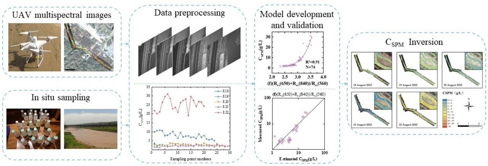
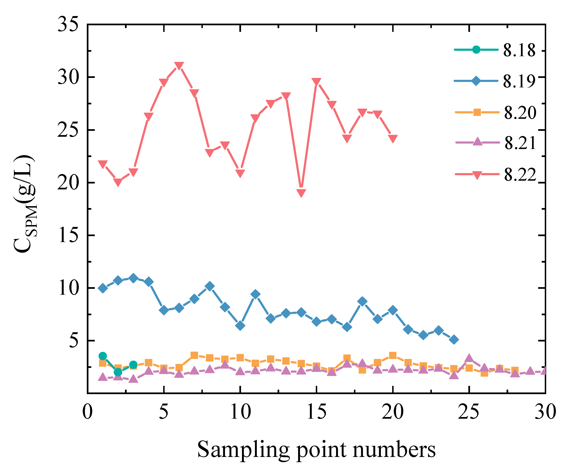
Therefore, the Wuding River, recognized as one of the principal sediment-laden tributaries of the Yellow River, was chosen as the study area. An experiment was conducted both before and after a summer rainfall event using multispectral UAV remote sensing technology in conjunction with in situ sampling, enabling CSPM inversion in this context. This study aims to address the following inquiries: What is the suitability and accuracy of existing CSPM inversion models when applied to the Wuding River, characterized by its extreme turbidity? How to develop a new high-precision inversion model if existing models have proved unsuitable? And, what are the spatial and temporal patterns of CSPM in the Wuding River before and after the occurrence of a heavy rainfall?
By addressing the aforementioned questions, we offer valuable technical and methodological insights into UAV remote sensing monitoring of CSPM in such challenging water bodies. These findings are expected to provide critical support for achieving precise sediment management in the Yellow River and contributing to the objective of high-quality development within the Yellow River Basin.

2. Materials and Methods

2.1. Study Area

The Wuding River, a primary tributary of the Yellow River, is situated in the northern region of Shaanxi Province, China. It spans approximately 491 km, coursing through multiple counties, including Dingbian, Jingbian, Mibi, Suide, and Qingjian before merging into the Yellow River in a northwest to southeast direction. The Wuding River Basin occupies a transitional zone between the Mao Wusu Desert and the Loess Plateau, with a watershed area accounting for 4.2% of the Yellow River Basin. It is characterized by loose soil, sparse vegetation, and extensive soil erosion, making it a significant source of coarse sediment to the Yellow River [23]. Despite its relatively limited runoff, averaging 1.53 billion m3 annually, which accounts for only 2.4% of the entire Yellow River Basin, the sediment transport from the Wuding River contributes significantly to the Yellow River’s sediment load, constituting 27.8% (calculated from the sediment transport data at the Dingjiagou and Longmen Stations). Notably, sediment transport within the Wuding River follows a predominantly seasonal pattern, with the majority occurring during the summer, amounting to 83% of the annual total.
In this study, we focused on a 4 km segment of the lower Wuding River, which serves as a representative sediment transport tributary of the Yellow River. This segment is situated in Yulin City, Shaanxi Province, precisely located at coordinates 110°4′30″E, 37°51′40″N. Field data collection took place from 18 August to 22 August 2022, primarily involving the acquisition of multispectral UAV images and in situ water sampling. A total of 105 sampling points were uniformly distributed within the river, as depicted in Figure 1. Detailed sampling information is provided in Table 2. Throughout the UAV flights, sky irradiance measurements were conducted using an ASD HandHeld 2 ground spectrometer (Analytica Spectra Devices., Inc., Boulder, CO, USA) to facilitate the calculation of UAV remote sensing reflectance.

2.2. Methods

The methodological process of this study primarily comprises field UAV data acquisition and in situ ground sampling, computation of remote sensing reflectance for river water bodies, laboratory determination of CSPM at designated sample points, model calibration and validation, and subsequent CSPM inversion and spatial–temporal variation analysis, as illustrated in Figure 2.

2.2.1. In Situ Sampling

Ground sample points were evenly distributed longitudinally along the river. Water samples were collected at the riverbank and bridge edges using a 5 L metal water collector, while samples from the central river were obtained using an unmanned aerial vehicle (UAV). All collected samples were preserved in plastic bottles and promptly stored at 4 °C. Simultaneously, the coordinates of each sample point were recorded using a handheld GPS device.
On the day of collection, water samples were filtered using pre-burned and pre-weighed GF/F membranes and stored at −20 °C. In the laboratory, CSPM measurements were conducted by drying the membranes in an oven at 105 °C for four hours, followed by precise weighing using an electronic balance. Sample CSPM values were calculated by subtracting the weight of the blank membrane from the final weighing result, expressed in g/L.

2.2.2. UAV Data Acquisition and Processing

UAV Multispectral Image

We selected the DJI Phantom 4 multispectral UAV as the airborne platform for image data acquisition. This UAV is equipped with a frame sensor featuring five multispectral channels: Blue (450 ± 16 nm), Green (560 ± 16 nm), Red (650 ± 16 nm), Red Edge (730 ± 16 nm), and Near Infrared (840 ± 26 nm). A multispectral cosine sensor was used to measure the downwelling irradiance and record it within the image file.
Before the flight plan beginning, two distinct reference boards were manually photographed for in situ Remote Sensing Reflectance (Rrs) calibration. Throughout the experiment, a total of 3672 single-band images were acquired, resulting in a grand total of 18,360 images. These images possessed a resolution of 9 cm/pixel, effectively covering a river length of 3.92 km. The detailed instrument parameters and flight parameters are provided in Table 3.

Computing of Rrs of Water Bodies from Drone Data

Geometric correction, radiometric calibration, and mosaic were initially conducted using DJI Terra software. Subsequently, we derived terrestrial reflectance (ρ) from the images, relying on the downwelling irradiance data recorded by the cosine sensor within the images.
Furthermore, we calculated the water remote sensing reflectance ratio (Rrs) based on ρ, applying the water remote sensing reflectance formula. This calculation proceeded as follows:
Rrs = Lw/Ed
where Rrs represents the remote sensing reflectance (sr−1), Lw represents the off-water irradiance (W∙sr−1∙m−2), and Ed is the downwelling irradiance (W∙m−2).
Lw is calculated using the following formula:
Lw = LswrLsky
where Lsw is the total signal acquired by the UAV sensor (W∙sr−1∙m−2) and r is the Fresnel coefficient, which takes the value of 0.025. Lsky is the scattered light from the sky, which is measured by the FieldSpec HandHeld 2 ground spectrometer during the flight progress of the UAV. We selected multiple points and calculated the mean value to participate in the calculation.
Then, the above equation could be changed to:
Rrs = (LswrLsky)/Ed
When extracting the water body range, it was observed that the NDWI threshold segmentation method yielded unsatisfactory results for watershed extraction in the study area. To improve accuracy, this study incorporated the NDWI and red band (650 nm) Rrs for water body extraction.
In the preliminary extraction results of the water body obtained using the NDWI thresholding method, the NDWI was calculated using the following formula:
NDWI = (Rrs(560) − Rrs(840))/(Rrs(560) + Rrs(840))
To address the issue of roads and bridges being misidentified and partially confused with the water body (as shown in Figure 2a), we initially applied the NDWI threshold of NDWI ≥ 0.1 for water extraction. Subsequently, we utilized Rrs(650) to refine the water body range, setting a threshold value of 0.17 ≤ Rrs(650) ≤ 0.21. The results demonstrated a substantial enhancement in the accuracy of the extracted water body boundaries, effectively mitigating misclassifications involving roads, bridges, and bare land near the water body (as depicted in Figure 2b).

2.2.3. CSPM Model Development

Based on assessing the applicability of existing models, we proceeded to establish a more suitable CSPM inversion model based on the reflectance characteristics of each band in the UAV multispectral data. Subsequently, we validated this new model using the same methodology. Since the CSPM varies greatly from day to day, based on the 105 in situ sampling points, we divided the daily measured data into 70% for model development and 30% for model validation. This way, the model development and validation data can basically cover all concentration ranges.
Five existing empirical CSPM models, including single bands and band ratios, and one semi-analytical model were selected, including Liu’s [14], Doxaran’s 1 [19], Doxaran’s 2 [19], Espinoza-Villar’s [20], Ying’s [12], and QAA [13]. Their applicability was evaluated in the study area, with the model calibration using data from the sampling points in this study.
By analyzing the characteristics of the UAV reflectance curves and CSPM changes in this study, we attempted to develop a CSPM inversion model with six different input variables. These variables included two single bands, Single Band 1 (SB1) and Single Band 2 (SB2); one two-band combination, Two Band (TB); one band ratio, Band Ratio (BR); and two three-band combinations, Three Band 1 (TB1) and Three Band 2 (TB2).

2.2.4. Accuracy Evaluation

The coefficient of determination (R2), root mean square error (RMSE), and mean absolute percentage error (MAPE) were used for accuracy evaluation in this study [24]. The calculation formulas are:
R 2 = 1 ( y i y ^ i ) 2 ( y i y ¯ ) 2
R M S E = 1 n i = 1 n ( y ^ i y i ) 2
M A P E = 1 n i = 1 n | y ^ i y i y i | × 100 %
where y ¯ is the average of the measured dataset, y i denotes the measured value of the ith sample, and y ^ i is the estimated value.

3. Results

3.1. Measured CSPM and Spectral Characterization Analysis

Figure 3 shows the results of the laboratory measurements of CSPM of the sampling points, with an overall range of 1.27–31.18 g/L and a significant difference within five days. The highest CSPM was recorded on 22 August, with some of the sample points exceeding 30 g/L. On that day, the concentration varied widely among sample points, with a maximum of 31.18 g/L, a minimum of 19.08 g/L, and a mean concentration of 25.31 g/L, as summarized in Table 4. Conversely, the lowest CSPM was found on 21 August, with a narrower concentration range and less variability among sample points. Specifically, the maximum value and the minimum were 3.24 g/L and 1.27 g/L, and the mean value was 2.12 g/L.
The multispectral UAV Rrs results, shown in Figure 4, were significantly higher at 650 nm, 730 nm, and 840 nm than at 450 nm and 560 nm. With the increase of the CSPM at the sample point, the Rrs increased in all bands, and the curve was elevated overall.

3.2. CSPM Inversion Model Accuracy Evaluation

3.2.1. Existing CSPM Inversion Models

Six existing models were selected for evaluation, and the expressions and accuracy of the models after calibration are presented in Table 5. The results showed that the accuracy of Liu’s single band and Doxaran’s band ratio models were better, while the semi-analytical model QAA exhibited the lowest performance (R2 was 0.24 and RMSE was 10.09 g/L). Doxaran’s 1 model was the most effective, with an R2 value of 0.75, corresponding to an RMSE of 4.52 g/L and a MAPE of 82.29%.
However, as can be seen from Figure 5, several points—although closer to the 1:1 line in the high concentration range where CSPM is below 20 g/L—are more disrupt in the extremely high concentration range above 20 g/L. This indicates that while the models are applicable to the high concentration range, they are less accurate in the extremely high range, and the concentrations of most of the sample points are underestimated.

3.2.2. CSPM Inversion Models Based on Multispectral UAV Data

This study aimed to propose CSPM inversion models with several different input parameters, respectively, by analyzing the spectral characteristics of UAV. Firstly, 70% of the measured sample points were employed as the calibration dataset, and the best forms of the six models were determined by empirical regression. As illustrated in Figure 6, TB, SB1, SB2, and TB1 had the better linear fit in each of the fitting forms, but their performance varied greatly with the concentration range, and the fitting accuracy was poor in the extremely high concentration range. The results were summarized as follows. The exponential fit was the best among the fitting forms with TB2 as inputs, and the fitted model (TB2-EXP) with TB2 and CSPM had a relatively higher accuracy on the prediction set, with an R2 of 0.91, and a good correlation between high and extremely high concentrations. The results of the model validation and accuracy evaluation are shown in Figure 7 and Table 6, which shows that the TB2-EXP model validation accuracy is the highest (R2 of 0.83, RMSE of 3.73 g/L, and MAPE of 44.95%), both in comparison with the other five new models and the existing models in Section 3.2.1. Therefore, in this study, the TB2-EXP model was selected for CSPM inversion. See Appendix A for details.

3.3. UAV Image Inversion Based on TB2-EXP Model

Using the TB2-EXP model, the UAV data for the five days from 18 to 22 August were inverted to generate CSPM distribution maps for the entire river reach. As illustrated in Figure 8 and summarized in Table 7, the temporal CSPM varied significantly from day to day, with large differences in mean CSPM of 5.66 g/L, 6.01 g/L, 2.97 g/L, 1.86 g/L, and 10.73 g/L. This can be attributed to the fact that there were two rainfall events during the sampling process, which occurred on 18 August (16.5 mm) and 21 August (11.2 mm). The amount of rainfall on the 21st was less than that on the 18th, but it was shorter in duration and more intense. The CSPM exhibited an average increase of 0.35 g/L on 19 August, followed by a gradual decrease in CSPM on the following two days, with the average concentration on 21 August being the lowest in the five days. After a short period of intense rainfall that occurred on 21 August, the mean CSPM was elevated by 8.87 g/L on 22 August. It is evident that rainfall has a significant influence on CSPM, especially a short period of heavy rainfall can cause a rapid and significant increase in CSPM in a short period of time, and then gradually decrease in the following period of time. Spatially, the variation of concentration in the whole study area was not apparent.

4. Discussion

4.1. Applicability of New Models

Empirical and semi-empirical CSPM models have been applied to various inland waters with different concentration ranges and data sources, including satellite-based, airborne, and in situ sensors. Most of the models initially identify the most suitable wavelengths by CSPM and develop corresponding models to invert them accurately. However, these models were developed using different in situ measurement datasets. For example, the single-band model in [14] is suitable for the accurate estimation of CSPM in the range of 0–60 mg/L, so these models may not be suitable for the estimation of other ranges of CSPM. In contrast, the CSPM in this study was up to 30 g/L, and the extremely high CSPM is rarely found in the existing literature. As verified using the dataset of this study, the existing models are no longer applicable, likely due to the measured CSPM exceeding the range of applicability of these models, so we established new models based on the spectral characteristics of the water body in the case of extremely high CSPM.
Since the increase of CSPM will make the Rrs of the water body increase significantly in the visible range, the visible band signal will be saturated after reaching a certain concentration, and then the characteristic band that can reflect the CSPM will be red-shifted to the near-infrared or even the mid-infrared band [25]. Therefore, using the near-infrared band as the input parameter of the model can achieve better simulation accuracy in the case of extremely high CSPM. This is corroborated by the relatively accurate performance of established models when the input parameters include Rrs (840), such as Liu’s in Table 8. The band ratio method can be an inverse modeling by selecting the reflectance ratio calculation ratio of the band combination with the highest correlation among all possible band combinations [26]. Moreover, based on the characteristics of the sample UAV spectral curve with CSPM, our TB2-EXP model uses the ratio of the higher Rrs of 650 nm to the lower one of 560 nm, in addition to the Rrs (840), as model input parameters to highlight the characteristics of the Rrs at extremely high CSPM, which makes the input parameters better correlated with CSPM and suitable for model development.
In this study, 70% of the data were used for inversion model calibration, and the correlation with the Rrs was established by randomly sampling five days of measured data. The aim is to make the CSPM range cover 1–30 g/L and to build a model that can be applied to a wider range of concentrations to improve the applicability of the model. The existing model used in Section 3.2.1 and the new model established in Section 3.2.2 were validated in two concentration ranges—high concentration (CSPM < 20 g/L) and extremely high concentration (CSPM > 20 g/L). The validation results, as shown in Table 8, indicated that the highest R2 of the existing models in the high concentration range was 0.56, the RMSE was 1.26 g/L, and the MAPE was 36.89%, while the R2 of the TB2-EXP model was 0.72, the RMSE was 1.67 g/L, and the MAPE was 44.95%. The highest R2 of the existing model in the extremely high concentration range was 0.36, RMSE was 9.52 g/L, and MAPE was 11.47%, while the R2 of the new model was 0.65, RMSE was 6.20 g/L, and MAPE was 12.37%. In comparison, the accuracy of the new model we developed was significantly improved compared with the existing models, both overall and in the high and extremely high concentration ranges. It is clear that the TB2-EXP model performs significantly better than those in the existing literature and reflects the trend of CSPM well. It is worth noting that MAPE in high concentration is 40.68% and in extremely high concentration is 12.37%. After calculating the residuals (Figure 9), there are some overestimations in many of the sample points in the high concentration range, leading to an overestimation in the overall range. This suggests that the model has lost some of its ability to accurately predict in a high concentration range in order to ensure prediction accuracy in an extremely high concentration region. Therefore, in future research, we could first try developing the models based on different CSPM gradients. In addition, expanding the sampling datasets would be necessary. The summer rainy season period causes CSPM to peak throughout the year. To build a widely applicable model, additional sampling in different seasons would be needed to obtain measured data in different concentration gradients.

4.2. Advantages and Prospects of Remote Sensing on a UAV

The Yellow River, as one of the rivers with the highest sediment content in the world, derives 90% of its sediment from the Loess Plateau in its middle reaches [27]. The wind-formed loess, which can be up to tens or even hundreds of meters thick, has special physicochemical properties. Although the soil structure has high strength when dry, it will rapidly disintegrate when exposed to water, resulting in soil erosion. Thus, short-term strong rainfall is the main sediment-producing mechanism in the middle reaches of the Yellow River, and the effect of precipitation on sediment transport gradually increases with the rising of precipitation intensity [23,28,29,30,31]. Therefore, it is of great significance to monitor the changes of CSPM in the Yellow River and its main sediment-producing tributaries after rainfall events.
This study shows that the occurrence of short-term heavy rainfall can lead to rapid changes in river CSPM. Taking the Baijiachuan hydrological station of the Wuding River as an example, Figure 10a illustrates the in situ sediment content dataset collected in August 2016, which shows that the daily change of sediment of the Wuding River is more obvious in a month. The Sentinel 2 satellite can provide high spatial resolution (10 m) remote sensing images, and its revisit cycle is five days. Assuming that it can successfully collect valid data every five days and accurately monitor the sediment content, the data in Figure 10a were resampled by Sentinel 2; the revisit cycle is shown in Figure 10b. However, the cloudless available Sentinel 2 images actually downloaded from the ESA website are those of 7 and 27 August, and the sediment content obtained by the Sentinel 2 satellite is shown in Figure 10c. Figure 10d and Table 9 demonstrate the sediment content of different sampling principles. It can be seen that the reduction in datasets leads to a decline in monitoring accuracy. Specifically, the maximum monitored sediment content dropped from 101 kg/m3 to 32.3 kg/m3, and the mean value was changed from 26.42 kg/m3 to 36.45 kg/m3, which is a significant decrease in monitoring accuracy. Therefore, judging from the changes of river sediment before and after rainfall in this study, if only satellite remote sensing is used for monitoring, we should be careful of overestimation or underestimation of sediment content on a monthly or annual scale due to the lack of data. On the contrary, UAV platforms are not obscured by clouds, can acquire high-quality image data under cloudy conditions, etc., and can be flown at daily or even hourly intervals as needed [32]. Thus, UAV remote sensing becomes an effective method to provide an efficient means of monitoring rapid changes in river sediment.
When collecting UAV data, challenges such as sun glint, which can result from specular reflection and water movement, may affect the calculation of Rrs [33]. Therefore, we try to avoid direct sunlight at noon and select UAV flights with low wind speeds, but because it is not possible to avoid sun glint completely, we need to try an effective method to remove it. There are already many atmospheric correction methods that can improve this problem, and they have been applied in many satellites [34,35,36,37,38]. However, most of the atmospheric correction methods in the existing literature for satellite remote sensing are based on the wavelength bands and optical parameters of the satellite sensors, which makes it difficult to migrate them to UAVs. The theory of correction for sun glint is usually based on the fact that the Rrs of water is close to zero in the ultraviolet and the near-infrared band of 800–900 nm, when non-zero values at these wavelengths are the result of sun glint [39]. Therefore, sun glint corrections can be made by this theory to obtain accurate spectra [40]. However, for the extremely turbid waters in our study, the reflectance at these wavelengths is usually non-zero because of the presence of the water’s own spectral signal. It can also be seen in the spectral curves in Figure 4 that the Rrs is over 0.1 at wavelengths around 840 nm. It is not reasonable to use this type of correction. In low-altitude UAV remote sensing, the effect of atmospheric signals is almost negligible [41]. There are some sun glint pixels in the UAV images; however, due to the uncertainty of the atmospheric correction algorithms, the other normal pixels may be corrected and the overall accuracy may not be as good as the uncorrected results. Since there is currently no suitable UAV atmospheric correction algorithm to remove sun glint, we avoided selecting pixels with sun glint in both sampling and model development so that the calibration of the model is not affected. In future research, algorithms for solving sun glint issues have to be developed in order to obtain more accurate CSPM mapping results [33].
Another common challenge encountered in UAV data is the presence of bright and dark stripes, as depicted in Figure 11. This phenomenon arises from the fact that when a rotary-wing UAV is moving forward, the fuselage has a certain inclination (pitch angle) in the horizontal direction in order to obtain forward power. When the UAV route transforms, the solar altitude angle changes with respect to the plane where the cosine sensor is located on the top and which is rigidly connected to the fuselage. This shift in observational geometry of the sensor results in the appearance of bright and dark stripes in the images. To minimize this effect, future route planning for data collection on sunny days should consider positioning the UAV heading perpendicular to the solar azimuth, thereby improving the quality of raw data.

5. Conclusions

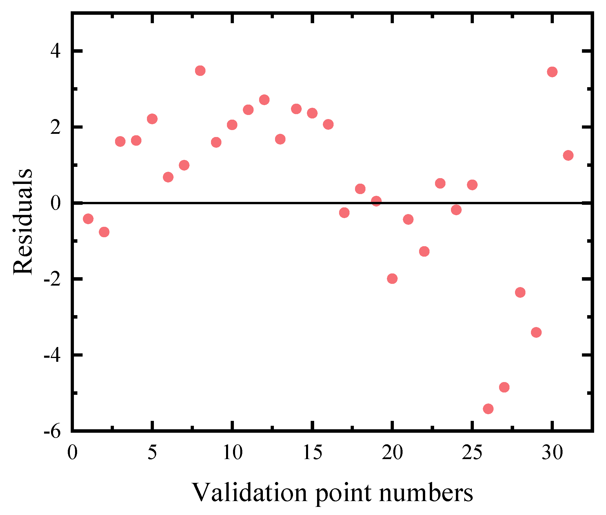
In this study, we conducted a CSPM inversion study in the extremely turbid Wuding River using UAV multispectral remote sensing technology. The results showed that the accuracy of the existing empirical or semi-analytical models was low due to the fact that the CSPM was out of the applicable range, particularly in the case of extremely high concentration (CSPM > 20 g/L). The newly developed model TB2-EXP significantly improved the accuracy of CSPM estimating (overall R2 of 0.83, RMSE of 3.73 g/L, MAPE of 44.95%). And, the performance of the model was especially good under the condition of extreme turbidity (CSPM > 20 g/L) (R2 of 0.65, RMSE of 6.20 g/L, MAPE of 12.37%). From the spatial inversion results, the changes of CSPM in the study area were obvious within five days, especially between 21 and 22 August, where the average CSPM increased significantly from 1.86 g/L to 10.73 g/L within ten hours after the heavy rainfall in the evening of the 21st day. This demonstrates the effectiveness of UAVs in monitoring significant CSPM changes over short durations, even under poor weather conditions. This study validated that the new proposed CSPM inversion model is well suited for remote sensing monitoring of extremely turbid rivers, such as the main tributaries of the Yellow River, which demonstrated the potential of multispectral UAVs in CSPM monitoring of narrow rivers. In the future, the sampling point data can continue to be supplemented to increase the robustness and applicability of the CSPM inversion model.

Author Contributions

Conceptualization, X.G. and Y.Z.; data collection, Y.Z., X.G., P.Z. and D.Z.; data preprocessing, Y.Z., X.G. and X.C.; writing, Y.Z.; guidance and opinions, X.G. and H.D. All authors have read and agreed to the published version of the manuscript.

Funding

This research was funded by the National Natural Science Foundation of China, grant number U2243205, and the Scientific Research Program funded by the Education Department of the Shaanxi Provincial Government, grant number 22JK0578.

Data Availability Statement

Data are contained within the article.

Conflicts of Interest

Author Xin Chen was employed by Shimadzu (China) Co., Ltd. The remaining authors declare that the research was conducted in the absence of any commercial or financial relationships that could be construed as a potential conflict of interest.

Appendix A

Table A1. Fitting forms of the new models, including linear, power, and exponential.
Input Parameters (x)ModelsExpressionsR2
R r s ( 650 ) linear C S P M = 62.5 R r s ( 650 ) 0.59428 0.69
power C S P M = 58.64 R r s ( 650 ) 0.99 0.68
exponential C S P M = exp 7.06236 R r s ( 650 ) 0.27
R r s ( 730 ) linear C S P M = 71.8 R r s ( 730 ) 1.15 0.62
power C S P M = 68.56 R r s ( 730 ) 1.03 0.6
exponential C S P M = 0.19 × 10⁸ R r s ( 730 ) 0.2
R r s ( 560 ) + R r s ( 840 ) linear C S P M = 38.67 ( R r s ( 560 ) + R r s ( 840 ) ) 0.8248 0.74
power C S P M = 36.34 ( R r s ( 560 ) + R r s ( 840 ) ) 1.0 0.67
exponential C S P M = 28 39.55 × 0.025 R r s ( 560 ) + R r s ( 840 ) 0.7
R r s ( 650 ) R r s ( 450 ) linear C S P M = 20.84 R r s ( 650 ) R r s ( 450 ) 43.4 0.63
power C S P M = 0.055 R r s ( 650 ) R r s ( 450 ) 5.28 0.75
exponential C S P M = 1618 1662 × 0.99 R r s ( 650 ) R r s ( 450 ) 0.63
( R r s ( 560 ) + R r s ( 650 ) )
× R r s ( 840 )
linear C S P M = 68.09 ( ( R r s ( 560 ) + R r s ( 650 ) )
× R r s ( 840 ) ) + 4.19
0.57
power C S P M = 1068 ( ( R r s ( 560 ) + R r s ( 650 ) ) × R r s ( 840 ) ) 9.9 0.48
exponential C S P M = 238 × 0.0187 ( R r s ( 560 ) + R r s ( 650 ) ) × R r s ( 840 ) ) 0.49
R r s ( 650 ) + R r s ( 840 ) R r s ( 560 ) linear C S P M = 21.08 R r s ( 650 ) + R r s ( 840 ) R r s ( 560 ) 54.11 0.69
power C S P M = 0.0039 R r s ( 650 ) + R r s ( 840 ) R r s ( 560 ) 6.87 0.73
exponential C S P M = 0.000806 × 19.51 R r s ( 650 ) + R r s ( 840 ) R r s ( 560 ) 0.91

References

  1. Wang, S.; Fu, B.; Piao, S.; Lü, Y.; Ciais, P.; Feng, X.; Wang, Y. Reduced sediment transport in the Yellow River due to anthropogenic changes. Nat. Geosci. 2016, 9, 38–41. [Google Scholar] [CrossRef]
  2. Wang, H.; Wu, X.; Bi, N.; Li, S.; Yuan, P.; Wang, A.; Syvitski, J.; Saito, Y.; Yang, Z.; Liu, S.; et al. Impacts of the dam-orientated water-sediment regulation scheme on the lower reaches and delta of the Yellow River (Huanghe): A review. Glob. Planet. Chang. 2017, 157, 93–113. [Google Scholar] [CrossRef]
  3. Gholizadeh, M.H.; Melesse, A.M.; Reddi, L. A Comprehensive Review on Water Quality Parameters Estimation Using Remote Sensing Techniques. Sensors 2016, 16, 1298. [Google Scholar] [CrossRef] [PubMed]
  4. Al-Fahdawi, A.; Rabee, A.M.; Al-Hirmizy, S.M. Water quality monitoring of Al-Habbaniyah Lake using remote sensing and in situ measurements. Environ. Monit. Assess. 2015, 187, 1–11. [Google Scholar] [CrossRef] [PubMed]
  5. Harvey, E.T.; Kratzer, S.; Philipson, P. Satellite-based water quality monitoring for improved spatial and temporal retrieval of chlorophyll-a in coastal waters. Remote Sens. Environ. 2015, 158, 417–430. [Google Scholar] [CrossRef]
  6. Ran, Q.H.; Zong, X.Y.; Ye, S.; Gao, J.H.; Hong, Y.Y. Dominant mechanism for annual maximum flood and sediment events generation in the Yellow River basin. Catena 2020, 187, 104376. [Google Scholar] [CrossRef]
  7. Zhong, Y.F.; Wang, X.Y.; Xu, Y.; Wang, S.Y.; Jia, T.Y.; Hu, X.; Zhao, J.; Wei, L.F.; Zhang, L.P. Mini-UAV-Borne Hyperspectral Remote Sensing from observation and processing to applications. IEEE Geosci. Remote Sens. Mag. 2018, 6, 46–62. [Google Scholar] [CrossRef]
  8. Moses, W.J.; Gitelson, A.A.; Perk, R.L.; Gurlin, D.; Rundquist, D.C.; Leavitt, B.C.; Barrow, T.M.; Brakhage, P. Estimation of chlorophyll-a concentration in turbid productive waters using airborne hyperspectral data. Water Res. 2012, 46, 993–1004. [Google Scholar] [CrossRef]
  9. Ma, R.; Tang, J.; Dai, J. Bio-optical model with optimal parameter suitable for Taihu Lake in water colour remote sensing. Int. J. Remote Sens. 2006, 27, 4305–4328. [Google Scholar] [CrossRef]
  10. Ahn, Y.H.; Moon, J.E.; Gallegos, S. Development of Suspended Particulate Matter Algorithms for Ocean Color Remote Sensing. Korean J. Remote Sensing 2001, 4, 285–295. [Google Scholar]
  11. Nechad, B.; Ruddick, K.G.; Park, Y. Calibration and validation of a generic multisensor algorithm for mapping of total suspended matter in turbid waters. Remote Sens. Environ. 2010, 114, 854–866. [Google Scholar] [CrossRef]
  12. Ying, H.T.; Xia, K.; Huang, X.X.; Feng, H.L.; Yang, Y.H.; Du, X.C.; Huang, L.J. Evaluation of water quality based on UAV images and the IMP-MPP algorithm. Ecol. Inform. 2021, 61, 101239. [Google Scholar] [CrossRef]
  13. Jiang, D.; Matsushita, B.; Pahlevan, N.; Gurlin, D.; Lehmann, M.K.; Fichot, C.G.; Schalles, J.; Loisel, H.; Binding, C.; Zhang, Y.L.; et al. Remotely estimating total suspended solids concentration in clear to extremely turbid waters using a novel semi-analytical method. Remote Sens. Environ. 2021, 258, 112386. [Google Scholar] [CrossRef]
  14. Liu, Y.; Xia, K.; Feng, H.; Fang, Y. Inversion of water quality elements in small and micro-size water region using multispectral image by UAV. Acta Scientiae Circumstantiae 2019, 39, 1241–1249. [Google Scholar]
  15. Olivetti, D.; Roig, H.; Martinez, J.M.; Borges, H.; Ferreira, A.; Casari, R.; Salles, L.; Malta, E. Low-Cost Unmanned Aerial Multispectral Imagery for Siltation Monitoring in Reservoirs. Remote Sens. 2020, 12, 1855. [Google Scholar] [CrossRef]
  16. Giardino, C.; Bresciani, M.; Valentini, E.; Gasperini, L.; Bolpagni, R.; Brando, V.E. Airborne hyperspectral data to assess suspended particulate matter and aquatic vegetation in a shallow and turbid lake. Remote Sens. Environ. 2015, 157, 48–57. [Google Scholar] [CrossRef]
  17. Olmanson, L.G.; Brezonik, P.L.; Bauer, M.E. Airborne hyperspectral remote sensing to assess spatial distribution of water quality characteristics in large rivers: The Mississippi River and its tributaries in Minnesota. Remote Sens. Environ. 2013, 130, 254–265. [Google Scholar] [CrossRef]
  18. Zang, C.; Shen, F.; Yang, Z. Aquatic environmental monitoring of inland waters based on UAV hyperspectral remote sensing. Remote Sens. Nat. Res. 2021, 33, 45–53. [Google Scholar]
  19. Doxaran, D.; Castaing, P.; Lavender, S.J. Monitoring the maximum turbidity zone and detecting fine-scale turbidity features in the Gironde estuary using high spatial resolution satellite sensor (SPOT HRV, Landsat ETM+) data. Int. J. Remote Sens. 2006, 27, 2303–2321. [Google Scholar] [CrossRef]
  20. Espinoza-Villar, R.; Martinez, J.M.; Armijos, E.; Espinoza, J.C.; Filizola, N.; Dos Santos, A.; Willems, B.; Fraizy, P.; Santini, W.; Vauchel, P. Spatio-temporal monitoring of suspended sediments in the Solimoes River (2000–2014). C. R. Geosci. 2018, 350, 4–12. [Google Scholar] [CrossRef]
  21. Arango, J.G.; Nairn, R.W. Prediction of Optical and Non-Optical Water Quality Parameters in Oligotrophic and Eutrophic Aquatic Systems Using a Small Unmanned Aerial System. Drones 2019, 4, 1. [Google Scholar] [CrossRef]
  22. Yang, Z.; Lu, X.P.; Wu, Y.B.; Miao, P.J.; Zhou, J.L. Retrieval and model construction of water quality parameters for UAV hyperspectral remote sensing. Sci. Surv. Mapp. 2020, 45, 60–64. [Google Scholar]
  23. Li, M.N.; Yu, K.X.; Zhang, X.; Yang, Z.; Li, P.; Li, Z.B. Variation Characteristics of Extreme Sediment and Its Influencing Factors in the Wuding River Basin. J. Soil Water Conserv. 2023, 37, 114–122. [Google Scholar]
  24. Wei, L.F.; Wang, Z.; Huang, C.; Zhang, Y.; Wang, Z.X.; Xia, H.Q.; Cao, L.Q. Transparency Estimation of Narrow Rivers by UAV-Borne Hyperspectral Remote Sensing Imagery. IEEE Access 2020, 8, 168137–168153. [Google Scholar] [CrossRef]
  25. Yafei, L.; David, D.; Kevin, R.; Fang, S.; Bernard, G.; Liwen, Y.; Haijun, H. Saturation of water reflectance in extremely turbid media based on field measurements, satellite data and bio-optical modelling. Opt. Express 2018, 26, 10435. [Google Scholar]
  26. Warren, M.A.; Simis, S.G.H.; Martinez-Vicente, V.; Poser, K.; Bresciani, M.; Alikas, K.; Spyrakos, E.; Giardino, C.; Ansper, A. Assessment of atmospheric correction algorithms for the Sentinel-2A MultiSpectral Imager over coastal and inland waters. Remote Sens. Environ. 2019, 225, 267–289. [Google Scholar] [CrossRef]
  27. Wang, H.; Yang, Z.S.; Saito, Y.; Liu, J.P.; Sun, X.X.; Wang, Y. Stepwise decreases of the Huanghe (Yellow River) sediment load (1950–2005): Impacts of climate change and human activities. Glob. Planet. Chang. 2007, 57, 331–354. [Google Scholar] [CrossRef]
  28. Jiao, J.; Wang, Z.; Wei, Y.; Su, Y.; Cao, B.; Li, Y. Characteristics of erosion sediment yield with extreme rainstorms in Yanhe Watershed based on field measurement. Tran. Chin. Soc. Agric. Eng. 2017, 33, 159–167. [Google Scholar]
  29. Cheng, Y.; He, H.M.; Cheng, N.N.; He, W.M. The Effects of Climate and Anthropogenic Activity on Hydrologic Features in Yanhe River. Adv. Meteorol. 2016, 2016, 5297158. [Google Scholar] [CrossRef]
  30. Chen, R.; Wen, Y.; Gao, P.; Mu, X.; Sun, W. Comparative analysis of flow and sediment characteristics of the Yanhe River under extreme rainfall conditions and research on influence factors. Act. Ecol. Sin. 2018, 38, 1920–1929. [Google Scholar]
  31. Arango, J.G.; Nairn, R.W. Prediction of Sediment Yield in the Middle Reaches of the Yellow River Basin under Extreme Precipitation. Front. Earth Sci. 2020, 8, 542686. [Google Scholar]
  32. Fráter, T.; Juzsakova, T.; Lauer, J.; Dióssy, L.; Rédey, K. Unmanned aerial vehicles in environmental monitoring—An efficient way for remote sensing. J. Environ. Sci. Eng. 2017, 4, 85–91. [Google Scholar] [CrossRef]
  33. Su, T.C. A study of a matching pixel by pixel (MPP) algorithm to establish an empirical model of water quality mapping, as based on unmanned aerial vehicle (UAV) images. Int. J. Appl. Earth Obs. Geoinf. 2017, 58, 213–224. [Google Scholar] [CrossRef]
  34. Braga, F.; Fabbretto, A.; Vanhellemont, Q.; Bresciani, M.; Giardino, C.; Scarpa, G.M.; Manfè, G.; Concha, J.A.; Brando, V.E. Assessment of PRISMA water reflectance using autonomous hyperspectral radiometry. ISPRS-J. Photogramm. Remote Sens. 2022, 192, 99–114. [Google Scholar] [CrossRef]
  35. Zhang, M.W.; Hu, C.M.; Cannizzaro, J.; English, D.; Barnes, B.B.; Carlson, P.; Yarbro, L. Comparison of two atmospheric correction approaches applied to MODIS measurements over North American waters. Remote Sens. Environ. 2018, 216, 442–455. [Google Scholar] [CrossRef]
  36. Steinmetz, F.; Deschamps, P.Y.; Ramon, D. Atmospheric correction in presence of sun glint: Application to MERIS. Opt. Express 2011, 19, 9783–9800. [Google Scholar] [CrossRef]
  37. Vanhellemont, Q.; Ruddick, K. Atmospheric correction of Sentinel-3/OLCI data for mapping of suspended particulate matter and chlorophyll-a concentration in Belgian turbid coastal waters. Remote Sens. Environ. 2021, 256, 112284. [Google Scholar] [CrossRef]
  38. Li, S.J.; Song, K.S.; Li, Y.; Liu, G.; Wen, Z.D.; Shang, Y.X.; Lyu, L.; Fang, C. Performances of Atmospheric Correction Processors for Sentinel-2 MSI Imagery Over Typical Lakes Across China. IEEE J. Sel. Top. Appl. Earth Observ. Remote Sens. 2023, 16, 2065–2078. [Google Scholar] [CrossRef]
  39. Kutser, T.; Vahtmäe, E.; Paavel, B.; Kauer, T. Removing glint effects from field radiometry data measured in optically complex coastal and inland waters. Remote Sens. Environ. 2013, 133, 85–89. [Google Scholar] [CrossRef]
  40. Tan, J.; Cherkauer, K.A.; Chaubey, I. Using hyperspectral data to quantify water-quality parameters in the Wabash River and its tributaries, Indiana. Int. J. Remote Sens. 2015, 36, 5466–5484. [Google Scholar] [CrossRef]
  41. Kwon, Y.S.; Pyo, J.; Kwon, Y.H.; Duan, H.T.; Cho, K.H.; Park, Y. Drone-based hyperspectral remote sensing of cyanobacteria using vertical cumulative pigment concentration in a deep reservoir. Remote Sens. Environ. 2020, 236, 111517. [Google Scholar] [CrossRef]
Figure 1. The geographic information in the Wuding River Basin (including DEM, land use type, soil type, and vegetation coverage) and the distribution of sampling points in the study area.
Remotesensing 15 05398 g001
Figure 2. Flowchart of the CSPM inversion methodology for this study ((a) is water body extraction result by NDWI, and (b) is the result by NDWI and Rrs(650)).
Remotesensing 15 05398 g002
Figure 3. Results of CSPM laboratory measurement.
Remotesensing 15 05398 g003
Figure 4. Rrs obtained from UAV images at each sample point. The color of the folded line represents the high or low CSPM at the point, which transitions from light yellow to reddish black with increasing concentration. The gray curve is the Rrs derived from the HH2 spectrometer. The reflectance trends of the UAV and HH2 roughly match, so the UAV Rrs can be used for subsequent modeling studies.
Remotesensing 15 05398 g004
Figure 5. Scatter plots of existing CSPM models’ calibration results (The input parameters are as follows. (a) Rrs(840)/Rrs(650); (b) (Rrs(650) + Rrs(730))/Rrs(560); (c) bbp(840); (d) Rrs(840); (e) Rrs(650)/Rrs(560); (f) Rrs(840)/Rrs(560). N is the number of model validation points).
Remotesensing 15 05398 g005
Figure 6. Regression analysis of the six models based on multispectral UAV data (The input parameters are as follows. (a) Rrs(650); (b) Rrs(730); (c) Rrs(560) + Rrs(840); (d) Rrs(650)/Rrs(450); (e) (Rrs(560) + Rrs(650)) × Rrs(840); (f) (Rrs(650) + Rrs(840))/Rrs(560). N is the number of model validation points).
Remotesensing 15 05398 g006
Figure 7. Validation results of estimated and measured values of six models based on multispectral UAV data (The input parameters are as follows. (a) Rrs(650); (b) Rrs(730); (c) Rrs(560) + Rrs(840); (d) Rrs(650)/Rrs(450); (e) (Rrs(560) + Rrs(650)) × Rrs(840); (f) (Rrs(650) + Rrs(840))/Rrs(560). N is the number of model validation points).
Remotesensing 15 05398 g007
Figure 8. Inversion results of CSPM for the UAV multispectral images.
Remotesensing 15 05398 g008
Figure 9. Residuals of validation of TB2-EXP model.
Remotesensing 15 05398 g009
Figure 10. Comparison of sediment content from field measurements and Sentinel 2 satellite monitoring. (a) is the measured in situ sediment content dataset, (b) is the sediment content data resampled by Sentinel 2 revisit cycle, (c) is the result of resampling by available Sentinel 2 data, and (d) is the boxplot of different sampling principles.
Remotesensing 15 05398 g010
Figure 11. Comparison of UAV imagery on 18 August (a) and 22 August (b).
Remotesensing 15 05398 g011
Table 1. Existing empirical and semi-analytical models for inverse CSPM.
Algorithm FormReferencesAreaCSPM RangeData Source
Single band C S P M R r s ( 840 ) [14]Donghu Lake, China0–60 mg/LUAV multispectral image
[15]The Paranoá and the Corumbá IV reservoirs, Brazil0–180 mg/LUAV multispectral image
C S P M R r s ( 440 ) [16]Lake Trasimeno, Italy2–6 mg/LAirborne hyperspectral data
C S P M R r s ( 705 ) [17]Mississippi River, United States0–50 mg/LAirborne hyperspectral data
C S P M R r s ( 733 ) [18]Chongming Island, China4–280 mg/LUAV hyperspectral image
Band ratio C S P M R r s ( 700 ~ 900 v i s i b l e ) [19]The Gironde estuary, France10–2000 mg/LSPOT1, 2, 3/Landsat7
C S P M R r s ( 650 560 ) [20]The Solimoes River, Peru20–240 mg/LMODIS
C S P M R r s ( 475 668 ) [21]Human-made ponds, United States0–8 mg/LUAV multispectral image
C S P M R r s ( 500 670 500 + 670 ) [22]Luoshan County Reservoir in Henan Province, China6–12 mg/LUAV hyperspectral image
Three-band algorithm C S P M R r s ( 650 + 730 560 ) [12]Qingshan Lake, China10–70 mg/LUAV multispectral image
QAA C S P M = A b b p + B [13]Nile River, AmazonRiver, and Yangtze River; Lake Victoria, Lake Qinghai,
Lake Turkana, and Lake Kasumigaura
1–1000 mg/LMERIS, OLCI
Nechad C S P M = A ρ ρ W 1 ρ W C ρ + B ρ ,
ρ W = π R r s
[11]Southern North Sea, Belgium0–100 mg/LMERIS, MODIS
Table 2. Sampling points and weather information.
DateSamplesWeatherPrecipitation in 24 h (mm)
18 August 20223Rainy day16.5
19 August 202224Overcast sky0
20 August 202228Cloudy day0
21 August 202230Rainy day11.2
22 August 202220Sunny day0
Note: Rainfall data are derived from the daily values of basic meteorological elements for national ground meteorological stations in China.
Table 3. Instrument parameters of the UAV and sensors.
ItemParameters
Instrument parametersWeight1.5 kg
Maximum flight altitude6000 m
Maximum flight speed50 km/h
Endurance27 min
Pixel1600 × 1300
Flight parametersFlight height170 m
Flight speed14 m/s
Spatial resolution0.09 m/pixel
Longitudinal overlap70%
Sidewise overlap50%
Table 4. Statistics of CSPM results.
Date in 2022SamplesCSPM (g/L)Variance (g/L)
MaxMinMean
18 August33.531.9972.740.39
19 August2410.925.097.912.79
20 August283.591.922.740.21
21 August303.241.272.120.16
22 August2031.1819.0825.3111.60
Table 5. Calibration results for six existing empirical and semi-analytical models.
ModelSpectral IndexAlgorithmsR2RMSE (g/L)MAPE
Liu’s R r s ( 840 ) C S P M = 60.25 × R r s ( 840 ) 0.61 0.714.8742.76%
Doxaran’s 1 R r s ( 650 ) R r s ( 560 ) C S P M = 0.0012 × 314.95 R r s ( 650 ) R r s ( 560 ) 0.754.5282.29%
Doxaran’s 2 R r s ( 840 ) R r s ( 560 ) C S P M = 0.49477 × R r s ( 840 ) R r s ( 560 ) 6.528 0.704.9580.85%
Espinoza-Villar’s R r s ( 840 ) R r s ( 650 ) C S P M = 48.59 R r s ( 840 ) R r s ( 650 ) 41.2 0.237.83>100%
Ying’s R r s ( 650 ) + R r s ( 730 ) R r s ( 560 ) C S P M = 0.0012 × 20.14 R r s ( 650 ) + R r s ( 730 ) R r s ( 560 ) 0.615.6692.08%
QAA b b p ( 840 ) r r s = R r s ( λ ) 0.52 + 1.7 R r s ( λ )
u ( λ ) = g 0 + g 0 2 + 4 × g 1 r r s ( λ ) 2 g 1 ,
b b p ( λ ) = u ( λ ) × a ( λ ) 1 u ( λ ) b b w ( λ )
C S P M = 0.651 b b p ( 840 ) + 0.095
0.2410.09>100%
Table 6. Expression of the CSPM inversion models based on multispectral UAV data and their accuracy evaluation results.
ModelSpectral IndexExpressionsR2RMSE (g/L)MAPE
SB1-LINEAR R r s ( 650 ) C S P M = 62.5 R r s ( 650 ) 0.59 0.704.9547.09%
SB2-LINEAR R r s ( 730 ) C S P M = 71.8 R r s ( 730 ) 1.26 0.714.8555.37%
TB-LINEAR R r s ( 560 ) + R r s ( 840 ) C S P M = 38.67 × ( R r s ( 560 ) + R r s ( 840 ) ) 0.82 0.724.5948.34%
BR-POWER R r s ( 650 ) R r s ( 450 ) C S P M = 0.055 R r s ( 650 ) R r s ( 450 ) 5.28 0.744.4470.82%
TB1-LINEAR ( R r s ( 560 ) + R r s ( 650 ) )
× R r s ( 840 )
C S P M = 68.09 ( ( R r s ( 560 ) + R r s ( 650 ) )
× R r s ( 840 ) ) + 4.19
0.496.3881.06%
TB2-EXP R r s ( 650 ) + R r s ( 840 ) R r s ( 560 ) C S P M = 0.00081 × 19.51 R r s ( 650 ) + R r s ( 840 ) R r s ( 560 ) 0.833.7344.95%
Table 7. Statistics of inversion results.
DateMaximum (g/L)Minimum (g/L)Mean (g/L)Standard Deviation (g/L)
18 August8.762.775.660.92
19 August9.223.246.011.01
20 August3.152.802.970.09
21 August5.270.431.861.04
22 August27.651.1210.734.73
Table 8. Prediction accuracies of the six existing models and the TB2-EXP model in different concentration ranges.
ClassNameHigh CSPM (<20 g/L)Extremely High CSPM (>20 g/L)
R2RMSE (g/L)MAPER2RMSE (g/L)MAPE
Existing modelsLiu’s0.561.2636.89%<013.5017.02%
Doxaran’s 1<02.4277.06%0.3611.5415.17%
Doxaran’s 20.452.9476.89%0.369.5211.47%
Espinoza-Villar’s0.031.93>100%0.0216.3824.95%
IMP-MPP0.233.72>100%<012.4615.77%
QAA0.032.7442.45%<024.1437.71%
TB2-EXPTB2-EXP0.721.6740.68%0.656.2012.37%
Table 9. Sediment transport statistics from field measurements and Sentinel 2 satellite monitoring.
DatasetMaximum (kg/m3)Minimum
(kg/m3)
Mean (kg/m3)Sum (kg/m3)
In situ101026.42818.97
Systematic sampling 56.7021.57129.44
Available Sentinel 232.320.336.4552.6
Disclaimer/Publisher’s Note: The statements, opinions and data contained in all publications are solely those of the individual author(s) and contributor(s) and not of MDPI and/or the editor(s). MDPI and/or the editor(s) disclaim responsibility for any injury to people or property resulting from any ideas, methods, instructions or products referred to in the content.

