Assessing Planet Nanosatellite Sensors for Ocean Color Usage

Abstract

An increasing number of commercial nanosatellite-based Earth-observing sensors are providing high-resolution images for much of the coastal ocean region. Traditionally, to improve the accuracy of normalized water-leaving radiance ($n{L}_w$) estimates, sensor gains are computed using in-orbit vicarious calibration methods. The initial series of Planet nanosatellite sensors were primarily designed for land applications and are missing a second near-infrared band, which is typically used in selecting aerosol models for atmospheric correction over oceanographic regions. This study focuses on the vicarious calibration of Planet sensors and the duplication of its red band for use in both the aerosol model selection process and as input to bio-optical ocean product algorithms. Error measurements show the calibration performed well at the Marine Optical Buoy location near Lanai, Hawaii. Further validation was performed using in situ data from the Aerosol Robotic Network—Ocean Color platform in the northern Adriatic Sea. Bio-optical ocean color products were generated and compared with products from the Visual Infrared Imaging Radiometric Suite sensor. This approach for sensor gain generation and usage proved effective in increasing the accuracy of $n{L}_w$ measurements for bio-optical ocean product algorithms.

1. Introduction

In recent years, commercial companies have increasingly been manufacturing and launching Earth-observing nanosatellites with radiometric sensors [1]. While the activity of building and launching orbiting remote sensing satellites has traditionally been funded and managed by government organizations, these new commercial players in the Earth-observing community are implementing technological innovations, such as reducing the size of the satellites and increasing the spatial resolution. This is one reason that the term “nanosatellite” is used to identify these types of sensors. While traditional polar-orbiting and geostationary satellites are large so as to accommodate several sensors with wide fields of view, the new smaller commercial sensors flown on nanosatellites typically have smaller fields of view. They create images of larger extents by flying several sensors in a constellation, with each individual sensor acquiring one segment of the overall scene. The data from these smaller image extents can then be mosaicked into a larger overall image area after acquisition. Many companies are emerging in the business of manufacturing and launching these nanosatellites [2]. For example, Planet flies their sensors, called “Doves” and “Super Doves”, in constellations they refer to as “Flocks” [2]. The activity presented here describes the tasks needed to calibrate and process these Planet Dove sensors, so they can be used for oceanographic remote sensing applications.

Before its data can be useful as input to bio-optical ocean color algorithms, the top-of-the-atmosphere radiance ($L_t$) measured with any satellite-based ocean-observing sensor needs to be transformed to water-leaving radiance $\left(L_w\right)$ and then normalized by coefficients including the cosine of the solar zenith angle to compute the normalized water-leaving radiance $\left(n{L}_w\right)$ [3,4,5]. To summarize, for each band, Equation (1) describes the radiance components of the top-of-the-atmosphere radiance ($L_t)$:

$$L_t=\left(L_r+L_a+t_{d_v}{L}_{wc}+t_{d_v}{L}_w\right)t_{g_v}{t}_{g_s},$$

(1)

where $L_r$ represents the Rayleigh scattering radiance, $L_a$ represents the aerosol radiance, $L_{wc}$ represents the surface whitecap radiance, and $L_w$ represents the water-leaving radiance. The $t_{d_v}$ term accounts for diffuse transmittance along the sensor view path from the surface to the satellite. Gaseous absorption in the Sun-to-surface and surface-to-sensor paths are accounted for in the $t_{g_s}$ and $t_{g_v}$ terms [4]. For clarity, $\lambda$, which represents the wavelength as an independent variable in most of these terms, is not included. However, this computation of $L_t$ is valid for each wavelength band of any radiometric sensor.

Rearranging these terms results in

$$L_w=\left(L_t-\left(L_r+L_a+{t_{d_v}L}_{wc}\right)\left(t_{g_v}{t}_{g_s}\right)\right){\left(t_{d_v}{t}_{g_v}{t}_{g_s}\right)}^{-1},$$

(2)

where all the terms on the right-hand side of the equation are known or can be computed except for $L_a$. The $L_r$ term has been modeled and stored in tables that are indexed with the sensor and solar zenith angles, as well as wind and wave information [6]. The diffuse transmittance and gas absorption along the radiance path can also be computed. Therefore, the estimation of $L_r$ and $L_a$ are the primary tasks performed in the atmospheric correction process.

Finally, the $n{L}_w$ can be computed as follows:

$$n{L}_w=L_w/\left({\mathrm{\mu }}_s{f}_s{t}_{d_s}{f}_b\right),$$

(3)

where ${\mu }_s$ represents the cosine of the solar zenith angle, $f_s$ represents the Earth–Sun distance correction, $t_{d_s}$ represents the diffuse transmittance along the solar view path, and $f_b$ represents the bidirectional reflectance correction [3].

There are challenges in using the Planet Dove datasets to generate bio-optical ocean color products. The first of these challenges is the difficulty in estimating the aerosol radiance, $L_a$. Historically, various methods have been suggested for estimating the $L_a$ term in Equation (2) [7,8]. This is part of the atmospheric correction process, which computes $L_r$ based on solar and sensor zenith and azimuth angles and $L_a$ to subtract them from the $L_t$ term in Equation (2).

A traditional approach to estimating $L_a$ for ocean remote sensing and the method that will be used in this discussion was proposed by Gordon and Wang in which two near-infrared (NIR) wavelength bands are used to select an aerosol model that is ultimately used to estimate $L_a$ [9]. This process assumes the signal from the larger NIR wavelength band, identified as “long_aerosol_wavelength”, can be used as a baseline measurement for identifying aerosol radiances. Since water absorbs almost fully in the NIR region, the assumption is that the signal from this band should have no scattering from a pure water medium and is a baseline for aerosol identification. Measurements above this baseline in the second NIR wavelength band, identified as “short_aerosol_wavelength”, are considered to represent aerosol scattering in the atmosphere and therefore representative of aerosol radiance. The ratio of reflectance in these NIR bands is used to select one of the eighty aerosol models from which $L_a$ is computed. These aerosol models are indexed by categories of relative humidity and particle size fraction. While the relative humidity information can be derived from climatology information, the particle size fraction category is inferred from the ratio of reflectance in these NIR bands.

Unfortunately, the Planet Dove sensors have only four bands, only one of which is truly in the NIR region. In addition, the Dove sensors have four series of sensor types: Series C, Series D, Series E, and Series F. Each of these sensor types has a different relative spectral response for its wavelength bands. Therefore, the wavelengths of the four bands are different for all the series except Series C and D.

Table 1. Wavelengths in nm for Dove bands for each sensor series.

Sensor	Blue Wavelength	Green Wavelength	Red Wavelength	NIR Wavelength
Series C	490	545	649	820
Series D	490	545	649	820
Series E	494	545	644	824
Series F	494	545	635	819

shows the difference in the bands’ wavelengths depending on the sensor series. The fourth band’s wavelengths are between 819 and 824 nm and the third band’s wavelengths are between 635 and 649 nm. Therefore, although the fourth band is a NIR band, the third band is in the red region of the light spectrum. However, even though this third “red” band is not a NIR band, it was used in the aerosol model selection process, and error analysis was performed on the atmospheric correction results. Of the Dove data purchased, there were more Series F Dove sensor scenes than scenes from all the other series put together. Since the description of the calibration and derived products is simplified when using only one set of wavelengths, all the Dove scenes used in this study were acquired from the Series F sensors.

The Automated Processing System (APS), developed at the Naval Research Laboratory (NRL), generates ocean color products from space-borne spectroradiometer sensors such as the Moderate Resolution Imaging Spectroradiometer (MODIS) [10], Visible Infrared Imaging Radiometer Suite (VIIRS) [11], Ocean and Land Colour Instrument (OLCI) [12], Geostationary Ocean Color Imager (GOCI) [13], and Advanced Himawari Imager (AHI) [14]. APS is based on and is consistent with the NASA SeaWiFS Data Analysis System (SeaDAS) code set [15]. Therefore, it uses established atmospheric correction and bio-optical algorithms endorsed by the ocean color community. APS extends the SeaDAS functionality by adding a batch-processing capability to sequence through and rapidly process many data files at a time and incorporates the capability to add and test new satellites and algorithms. APS generates a standard set of bio-optical image products, including chlorophyll concentration, water absorption, and backscattering coefficients. APS is designed to generate map-projected image data bases of satellite-derived products from a large flow of raw satellite input data in an automated fashion. Individual scenes are sequentially processed from the raw digital counts (Level 1) using standard parameters to a radiometrically and geometrically corrected (Level 3) product within several minutes. It further processes the data into several different temporal (daily, 8-day, monthly, yearly, and latest pixel) composites or averages (Level 4). These products are stored in the Hierarchical Data Format or NetCDF file format.

The atmospheric correction, vicarious calibration, and derivation of $n{L}_w$ was performed using APS. Due to the wavelength bands available, the chlorophyll computation for VIIRS was carried out using the chl_oci algorithm, while the chlorophyll computation for the Dove sensors was performed with the chl_oc2 algorithm. However, these two algorithms are very similar.

Information for each of the four initial Dove series was generated and stored in the APS-required data format. This includes information such as the band wavelength centers, solar irradiance, the Rayleigh optical depth, and the absorption and backscatter of pure water across the sensors’ spectral bandwidths. In order to transform $L_t$ into $n{L}_w$, APS uses the sensor information to perform standard aerosol model estimation methods, including the method proposed by Gordon and Wang [9].

The generation of $L_a$ is also important for in-orbit vicarious calibration activity, which is a process that computes sensor gains for each wavelength band [3,4,5]. The contribution of water-leaving reflectance is typically less than 10% of the reflectance of the combined ocean–atmosphere system, with the remainder caused by photons scattered by the atmosphere and reflected from the sea surface [16]. Therefore, adjusting the $L_t$ value through vicarious calibration is essential to increase the accuracy of the $L_w$ and $n{L}_w$ estimates by reducing the uncertainty due to atmospheric correction. During the vicarious calibration process, Equations (2) and (3) are solved to compute $L_w$ and $n{L}_w$. Then, the radiance and coefficient values of the terms on the right side of Equation (2) are recorded, and in situ $n{L}_w$ is substituted for the sensor-derived $n{L}_w$. Substituting the $n{L}_w$ term in Equation (3) with in situ $n{L}_w$ and inverting the equation, $L_{w_{insitu}}$ is computed in Equation (4). Using the $L_{w_{insitu}}$ term instead of the $L_w$ term in Equation (1), the “vicarious” $L_t$ or $v{L}_t$ is computed in Equation (5).

$$L_{w_{insitu}}={nL}_{w_{insitu}}\left({\mu }_s{f}_s{t}_{d_s}{f}_b\right)$$

(4)

$$v{L}_t=\left(L_r+L_a+t_{d_v}{L}_{wc}+t_{d_v}{L}_{w_{insitu}}\right)t_{g_v}{t}_{d_s}$$

(5)

The ratio of $v{L}_t / L_t$ provides a vicariously calibrated sensor gain for each wavelength band. Essentially, when multiplying the $L_t$ value with these gains, an adjustment occurs such that after atmospheric correction, the in situ $n{L}_w$ values are computed when applying Equations (2) and (3). Once these calibrated gains are computed at the in situ location, they can be used as gains for other scenes as well. Therefore, the accurate estimation of $L_a$ is important not only for deriving $n{L}_w$ but also for computing sensor gains through vicarious calibration.

2. Materials and Methods

The Planet Dove sensors’ raw $L_t$ data are distributed in GeoTIFF format along with companion XML files that contain additional metadata. The data in these GeoTIFF and XML files were converted to the NRL standard Level 1B (L1B) NetCDF file format designed as input for processing with APS. However, additional information needed to be computed and organized to allow APS to transform data from the Planet L1B files to bio-optical products stored in the Level 2 (L2) file. This information includes Rayleigh and aerosol model coefficient tables as well as other absorption and scattering coefficients integrated across the Dove sensors’ bandwidths.

Planet provides the relative spectral response (RSR) values for the four initial Planet Dove series [17]. These RSR tables start at 320 nm and increment by 10 nm every row down the table. The RSR measurements for each of the Dove’s four spectral bands are in the four accompanying columns. This table was interpolated to 1 nm rows to prepare for convolution with coefficients of geophysical characteristics stored at 1 nm intervals. It shows that the full-width half-maximum of the bandwidths are roughly 80, 110, 90, and 100 nm for the sequence of the four Dove bands.

The Hyperspectral Imager for the Coastal Ocean (HICO) sensor was a hyperspectral sensor developed by NRL and housed on the International Space Station (ISS) from late 2009 to 2014 [18]. It measured $L_t$ across the electromagnetic spectrum from 352 to 1079 nm at about 5.5 nm intervals. NASA generated the Rayleigh coefficient and aerosol tables for HICO at these 5.5 nm intervals so that HICO L1B datasets could be processed using SeaDAS and APS. The Dove sensor bands’ RSR values stored at 1 nm intervals were spectrally adjusted and convolved against the 5.5 nm HICO Rayleigh and aerosol model coefficients to generate Rayleigh and aerosol model coefficient tables for each of the bands in each of the 4 Dove sensor series. The RSR values at 1 nm intervals were also convolved against other coefficients stored a 1 nm intervals to generate Dove-specific coefficients for characteristics such as solar irradiance, Rayleigh optical depth, and the absorption and backscatter of pure water. These convolved Rayleigh and aerosol model tables and sensor-specific coefficients for each Dove band were used to process the Planet Dove scenes in APS.

In-orbit calibration is a standard procedure performed on space-borne sensors. As discussed earlier, vicarious calibration, which uses in situ data to compute sensor gains for each sensor band, is a common approach to performing in-orbit calibration. For this calibration to be effective, a well-maintained accurate in situ data source must be used to adjust the calibration. The Marine Optical System (MOS) located in the instrument bay of the Marine Optical Buoy (MOBY) has been the primary source for calibrating many space-borne radiometric sensors [19,20], and it provided the in situ data used for vicarious calibration of the Planet Dove sensors presented here. MOBY is stationed in the primarily Case 1 waters off Lanai, Hawaii. The MOS contains one spectrograph to measure ultraviolet and visible light from 340 nm to 640 nm and another spectrograph to measure light from 550 to 995 nm [21]. It measures upwelling radiance and downwelling irradiance and computes $L_w$ and $n{L}_w$. To generate sensor gains for the Dove sensors, vicarious calibration was performed by processing a subset of Dove scenes over the MOBY location. For the rest of this discussion, the MOBY/MOS sensor will simply be referred to as the MOBY sensor.

Even though in-orbit calibration is performed for the Dove sensors [22,23], in situ data for these calibration sites are primarily over land. Therefore, a vicarious calibration procedure using in situ MOBY data was performed to explore if it could lead to extracting information from water bodies. Each Dove sensor is identified by a “Sensor ID”, which is a unique string of four alphanumeric characters. However, since there are hundreds of Dove sensors, an obvious challenge is that not all Dove sensors pass over MOBY, and those that do pass over MOBY do not necessarily acquire scenes on an atmospherically clear day. Traditionally, the calibration of a space-borne sensor uses several scene-to-in situ data matches to compute gains. Then, the averages of these computed gains for each band are used as the established sensor gain set. This calibration approach was used for the Dove sensors. However, due to the limited data purchase, only five cloud-free scenes over MOBY were involved in the vicarious calibration. When new Dove scenes are processed, the gains from this average can be used in the APS processing. It should be noted that this assumes the Dove sensors are highly intercalibrated.

The 80 aerosol models are indexed by a 2-digit number. A number in the set [0, 1, 2, 3, 4, 5, 6, 7] represents one of eight relative humidity groups and is used in the tens digit of the index. The thresholds for these relative humidity groupings are 30, 50, 70, 75, 80, 85, 90, and 95 percent humidity. A number in the set [0, 1, 2, 3, 4, 5, 6, 7, 8, 9] represents the particle size fraction group and is used in the ones digit of the aerosol model index. The vicarious calibration process is primed with an aerosol model that most closely represents the aerosol model at the calibration location on the scene date. Relative humidity climatology data were used to select the index representing the relative humidity group. The relative humidity at MOBY was between 70 and 75 percent for all the calibration dates. Therefore, the corresponding relative humidity group was the third group, which, since it is a 0-indexed group number, is group number 2. Since the scenes to participate in the calibration were screened to include only pristine cloud-free days, a “good marine aerosol size” group was used to select the index representing the particle size group. The seventh-size particle group was used as a good maritime aerosol for clear days. Therefore, since the particle size group is a 0-based index group, the group number is 6, and the initial aerosol model used for the vicarious calibration is aerosol model 26.

In the initial phase of the processing, unity gains are used, which are defined as 1.0 for each wavelength band, and then through the vicarious calibration process, updated gains are computed for each wavelength band. There is variation across wave crest angles in the Dove images due to the sensor’s small spatial resolution. This requires a broader investigation into the whitecap radiance from Dove sensors. Therefore, the $L_{wc}$ whitecap radiance term was set to 0 in Equation (1) for this activity. Since Equation (1) has $L_a$ and $L_w$ terms, the vicarious calibration proceeds in two phases. The first phase was carried out using the initial aerosol model number, which was model 26 in the case of the Dove sensor calibration, along with unity gains, and new gains were generated for the NIR bands. Using these gains for the NIR bands stabilizes the $L_a$ term in the second phase. Once the NIR gains were set, the second phase was carried out using the calibrated NIR gains, along with unity gains for the visible bands, to estimate $L_w$ in those bands. The aerosol model number was not set to any value before the second phase. Instead, the calibrated NIR bands were used in the Gordon and Wang algorithm to select the aerosol model number, ideally resulting in the aerosol model initially used to prime the calibration. The $L_w$ term can be provided directly with the MOBY sensor. Another option is to use the solar zenith angle at the Dove scene’s acquisition time to transform the MOBY in situ $n{L}_w$ to a MOBY $L_w$. The in situ $L_w$ is substituted for the $L_w$ term in Equation (1) and is used along with the $L_r$ and $L_a$ terms to compute the vicarious $L_t$, or $v{L}_t$. An average of the $v{L}_t/L_t$ values covering the 5 × 5 pixels around the MOBY location for the five Dove scenes were used in the calibration process to compute the sensor gain values. In the second phase, this process was performed for each visible wavelength band, resulting in a sensor gain set for all bands.

There is an artifact of this approach in that during the Gordon and Wang atmospheric correction process, APS reduces the signal in the second NIR band, identified as “short_aerosol_wavelength”, toward 0. When using two true NIR bands, after atmospheric correction, the values in the two NIR bands of the L2 file will be close to 0. This is irrelevant in further processing since those NIR bands are not used in bio-optical ocean color algorithms. However, in the case of the Dove scenes, this is a significant drawback since the red band, used as the “short_aerosol_wavelength” band, is also needed for bio-optical algorithms. However, after atmospheric correction, there is almost no signal remaining in the red band to use in bio-optical ocean color algorithms.

To address the atmospheric correction’s impact on the red band’s $n{L}_w$ value being reduced toward 0, the red band in the L1B file was duplicated, allowing one of the duplicated bands to participate as the “short_aerosol_wavelength” band and the other to participate as the visible red band to be used in bio-optical ocean color algorithms. The creation of Dove’s standard NRL L1B data file was adjusted to duplicate the red band. This resulted in a 5-band Dove L1B file, with the 4th band being a duplication of the 3rd band. All supporting sensor data files were adjusted to accommodate this duplication. The computation in both the vicarious calibration and normal processing then used the fourth and fifth bands as the “short_aerosol_wavelength” and “long_aerosol_wavelength” bands, leaving the duplicated third band as a visible red band. The atmospheric correction process reduces the $n{L}_w$ values in the fourth and fifth bands toward 0. However, the third band is treated as a visible band, and its $n{L}_w$ values are computed along with the other visible bands. Vicarious calibration and error analysis were performed on both the four- and five-band Dove scene representations.

The waters at MOBY are Case 1 waters and are very clean and stable as a result of a deficiency of nutrients and biology. Additional error analysis was performed using other available in situ data to evaluate the use of these sensor gains to measure accurate $n{L}_w$ in Case 2 coastal waters. The AERosol Robotic NETwork (AERONET), a partnership between several organizations including NASA and PHOTON (Photometrie pour le Traitement Operationnel de Normalisation Satellitaire), established a collection of ground-based instruments to measure characteristics of aerosols in the atmosphere [24]. In addition to atmospheric measurements, the AERONET-OC (Ocean Color) instruments were modified to measure water-leaving radiance. These sensors are on a variety of structures, including platforms and piers. One of these platforms is the Acqua Alta Oceanographic Tower (AAOT) site in the Adriatic Sea 20 km southeast of Venice, Italy. These waters vary in the amount of non-algal particles (NAPs) and chromophoric dissolved matter (CDOM) [25,26]. As a result, they represent an example of Case 2 water.

Several Dove scenes over the AAOT site were included in the data purchase from Planet. Five relatively cloud-free scenes over AAOT were selected for validation purposes acquired on 21 April 2017, 27 November 2017, 6 December 2017, 19 December 2017, 21 December 2017. These scenes, along with their acquisition times, are shown in

Table 2. Dove, VIIRS, and AAOT acquisition times.

Date	Dove Acquisition	Initial AAOT Acquisition	VIIRS Acquisition	Second AAOT Acquisition
21 April 2017	09:14	09:22	11:35	12:16
27 November 2017	09:24	09:31	12:52	12:31
6 December 2017	09:24	09:34	11:42	11:34
19 December 2017	09:24	09:19	12:38	12:40
21 December 2017	09:24	09:41	12:00	12:20

. The “Initial AAOT Acquisition” column shows the closest AAOT acquisition time to the Dove acquisition time. The “Second AAOT Acquisition” column shows the closest AAOT acquisition time to the VIIRS acquisition time.

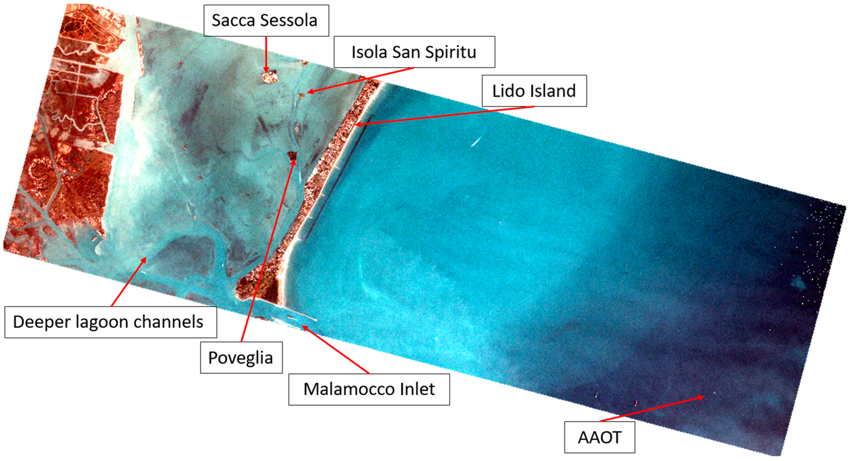
The Dove scenes cover the location within the Venetian Lagoon and the offshore waters beyond Lido Island, extending out to the AAOT platform. The example of the Dove image acquired on 6 December 2017 is shown in Figure 1. The location of the AAOT platform is shown in the lower right corner. The Malamocco inlet that connects the Venetian Lagoon to the Adriatic Sea appears at the southern edge of each of the scenes. Although this Dove scene does not capture Venice and the Grand Canal, the extent does capture several of the islands in the Venetian Lagoon and the marsh areas within the estuary just south of Venice, including the small islands of Sacca Sessola, Isola San Spiritu, and Poveglia, as well as other smaller islands. The deeper channels around the marshlands of the Venetian Lagoon are evident in the imagery. The image is reduced to fit in this document. The full scene, with its 3 m resolution, shows more detail in the features of the lagoon.

To perform the validation analysis, Dove products were compared with VIIRS products since the VIIRS sensor has been continuously calibrated with the MOBY sensor over time [27]. NRL performs a VIIRS vicarious calibration annually using data collected at MOBY.

Ocean color inherent and apparent optical properties (IOPs and AOPs), which quantify diffuse attenuation ($K_{\mathrm{d}}$), absorption ($a)$ and backscattering ($bb$), were generated. While VIIRS has the wavelength bands to generate IOPs using the QAA algorithm [28], the Dove sensors do not. Empirical algorithms have been used to compute diffuse attenuation coefficients [29,30]. IOP algorithms were also formalized and discussed within the International Ocean Colour Coordinating Group (IOCCG) [31]. Therefore, based on similar approaches to these algorithms, simplistic (one- or two-band) empirical algorithms were used to generate products such as $K_{\mathrm{d}}$, $a$, and $bb$ using relationships with derived chlorophyll [29,31]. So, while APS generated IOP estimates for the VIIRS data, these empirical algorithms were used to generate IOPs from the Dove sensors.

3. Results

Planet Dove scenes over MOBY were used in this vicarious calibration activity. After the calibration generated a new gain set, datasets were processed with both the unity and calibrated gains to compare the generated $n{L}_w$ values resulting from each gain set. Accuracy and error analyses using both the unity and calibrated gains were performed. All $n{L}_w$ measurements included are in units of $\mathrm{W}{\mathrm{m}}^{-2}{\mathrm{u}\mathrm{m}}^{-1} {\mathrm{s}\mathrm{r}}^{-1}$.

3.1. Vicarious Calibration

Dove scenes covering many different locations on the globe were purchased from Planet. Within this data repository, several Dove scenes were acquired over the MOBY location. These scenes were visibly screened to select cloud-free scenes. Ultimately, five Dove scenes were selected to participate in vicarious calibration.

The $n{L}_w$ values from MOBY, along with the corresponding values from the five Dove sensors, both with unity and vicariously calibrated gains, are shown in

Table 3. Planet Dove and MOBY nLw measurements in units of $\mathrm{W}{\mathrm{m}}^{-2}{\mathrm{u}\mathrm{m}}^{-1} {\mathrm{s}\mathrm{r}}^{-1}$ for four-band Dove scenes.

		$\mathbf{Planet} \mathit{n}{\mathit{L}}_{\mathit{w}}$ (nm)			$\mathbf{MOBY}\mathit{n}{\mathit{L}}_{\mathit{w}}$ (nm)
Date	Gains	494	545	635	494	545	635
17 February 2017	Unity	0.922	0.547	0.066	0.907	0.407	0.057
17 February 2017	Calibrated	0.909	0.407	−0.001	0.907	0.407	0.057
11 September 2017	Unity	1.401	0.691	0.217	0.966	0.429	0.063
11 September 2017	Calibrated	0.964	0.428	−0.004	0.966	0.429	0.063
22 October 2017	Unity	1.267	0.828	0.183	0.876	0.402	0.062
22 October 2017	Calibrated	0.876	0.402	−0.001	0.876	0.402	0.062
7 December 2017	Unity	1.237	0.685	0.152	0.891	0.399	0.061
7 December 2017	Calibrated	0.892	0.400	0.000	0.891	0.399	0.061
27 December 2017	Unity	1.684	1.023	0.240	0.905	0.394	0.060
27 December 2017	Calibrated	0.904	0.394	0.000	0.905	0.394	0.060

.

Two different types of error metrics were computed. First, the ratio of the Dove and MOBY $n{L}_w$ measurements were computed. The ratios that are over 1.0 indicate the amount that the Dove sensor overestimated the MOBY measurement. Ratios that are under 1.0 indicate the amount that the Dove sensor underestimated the MOBY measurement. These ratios were computed using results after processing with unity and calibrated gains. The comparison between the ratios from the unity and calibrated gains indicates improvement in the 494 and 545 nm wavelengths due to the calibration. These values are found in the “Ratio of $n{L}_w$ values” column of

Table 4. Ratios of Dove to MOBY $n{L}_w$ measurements for four-band Dove scenes and $RMSE$ in units of $\mathrm{W}{\mathrm{m}}^{-2}{\mathrm{u}\mathrm{m}}^{-1} {\mathrm{s}\mathrm{r}}^{-1}$.

Date	Gains	$\mathbf{Ratio} \mathbf{of} \mathbf{Dove} \mathbf{to} \mathbf{MOBY} \mathit{n}{\mathit{L}}_{\mathit{w}}$ Values			$\mathit{R}\mathit{M}\mathit{S}\mathit{E}$
		494 nm	545 nm	635 nm	Overall
17 February 2017	Unity	1.016	1.344	1.151	0.0814
17 February 2017	Calibrated	1.002	1.000	−0.013	0.0335
17 February 2017	Difference	0.014	0.344	1.164	0.0479
11 September 2017	Unity	1.451	1.611	3.431	0.3065
11 September 2017	Calibrated	0.998	0.997	−0.065	0.0390
11 September 2017	Difference	0.452	0.614	3.497	0.2675
22 October 2017	Unity	1.447	2.060	2.945	0.3414
22 October 2017	Calibrated	1.000	0.999	−0.018	0.0366
22 October 2017	Difference	0.447	1.061	2.963	0.3048
7 December 2017	Unity	1.388	1.714	2.496	0.2641
7 December 2017	Calibrated	1.000	1.000	−0.005	0.0354
7 December 2017	Difference	0.388	0.714	2.501	0.2287
27 December 2017	Unity	1.861	2.597	3.964	0.5873
27 December 2017	Calibrated	1.000	1.000	−0.005	0.0351
27 December 2017	Difference	0.862	1.597	3.968	0.5522

.

The equation for the overall root mean square error ($RMSE$) shown in Equation (6) was used to compute the second error metric, providing an overall assessment of the error in radiance units resulting from each of the two gain sets. The resulting RMSEs for each scene are also shown in the RMSE column of Table 4.

$$RMSE=\frac{\sqrt{\sum _{b=1}^3{\left(n{L_w}_{DOV{E}_b}-n{L_w}_{MOB{Y}_b}\right)}^2}}{3},$$

(6)

where b iterates through the three Dove visible bands, and the $n{L_w}_{DOVE}$ and $n{L_w}_{MOBY}$ terms identify the normalized water-leaving radiance of the DOVE and MOBY sensors.

The ratio of the $n{L}_w$ values in the “Calibrated” rows are nearer to 1.0 than the “Unity” rows, with some being slightly above and some slightly below 1.0. This indicates a reduced uncertainty between the calibrated Dove $n{L}_w$ estimate and the MOBY $n{L}_w$ measurements. The $RMSE$ column shows the $RMSE$ values before and after calibration in units of $\mathrm{W}{\mathrm{m}}^{-2}{\mathrm{u}\mathrm{m}}^{-1} {\mathrm{s}\mathrm{r}}^{-1}$. In many cases, the $RMSE$ is reduced by an order of magnitude, whereas the improvement in accuracy reaches close to a one-half unit of radiance. The “Difference” column presents the difference between the unity and calibrated ratios and reflects the impact of the calibration.

The calibration’s accuracy improvement for the 635 nm band shown in Table 4 was not as good as the improvement in the other two visible bands. The negative values for the red bands $n{L}_w$ ratios after calibration mean that the $n{L}_w$ estimates for the Dove sensor are negative, which is confirmed in Table 3. As previously mentioned, the reason for this is that during the atmospheric correction process, when using the red band as the “short_aerosol_wavelength”, the signal from that band determines how much of the signal should be identified as $L_a$ to be removed from the visible bands $L_t$. When this process was complete, the signal in the “short_aerosol_wavelength” band was reduced to close to 0. The fact is that in the Case 1 waters of Lanai, Hawaii, that house MOBY, there is minimal scattering of the $n{L}_w$ signal for this red band. So, $n{L}_w$ is naturally low in the 635 nm region of the light spectrum for these Case 1 waters. Through the atmospheric correction process, the $n{L}_w$ signal for this “short_aerosol_wavelength” band is identified as aerosol radiance and removed. Therefore, both the Dove and the MOBY $n{L}_w$ measurements are near 0. However, this is coincidental, simply an artifact of the atmospheric correction process and not because of a good estimation of water-leaving radiance in the red band. The reality is that some of these calibrated 635 nm $n{L}_w$ values are negative.

This is the reason why the third band in the L1B file was duplicated. It allowed one of these duplicated bands to be used as the “short_aerosol_wavelength” band in the atmospheric correction process and the other as a visible 635 nm band to use in deriving ocean color bio-optical products. This required the L1B file to be recreated as a five-band file with the red band duplicated in the third and fourth bands.

Once the five-band L1B files were generated for the MOBY scenes, the vicarious calibration process was performed again. This time, Band 4 was used as “short_aerosol_wavelength” for the aerosol model selection, and Band 3 was calibrated as a visible red band. The values of the Dove and MOBY $n{L}_w$ measurements using the five-band unity and calibrated gains are shown in

Table 5. Planet Dove and MOBY nLw measurements in units of $\mathrm{W}{\mathrm{m}}^{-2}{\mathrm{u}\mathrm{m}}^{-1} {\mathrm{s}\mathrm{r}}^{-1}$ for five-band Dove scenes.

Date	Gains	$\mathbf{Planet}\mathit{n}{\mathit{L}}_{\mathit{w}}$ (nm)			$\mathbf{MOBY} \mathit{n}{\mathit{L}}_{\mathit{w}}$ (nm)
		494	545	635	494	545	635
17 February 2017	Unity	0.922	0.547	0.066	0.907	0.407	0.057
17 February 2017	Calibrated	0.909	0.407	0.057	0.907	0.407	0.057
11 September 2017	Unity	1.410	0.691	0.217	0.966	0.429	0.063
11 September 2017	Calibrated	0.966	0.430	0.065	0.966	0.429	0.063
22 October 2017	Unity	1.267	0.828	0.183	0.876	0.402	0.062
22 October 2017	Calibrated	0.878	0.403	0.063	0.876	0.402	0.062
7 December 2017	Unity	1.237	0.685	0.152	0.891	0.399	0.061
7 December 2017	Calibrated	0.893	0.401	0.062	0.891	0.399	0.061
27 December 2017	Unity	1.684	1.023	0.240	0.905	0.394	0.060
27 December 2017	Calibrated	0.907	0.395	0.062	0.905	0.394	0.060

.

The accuracy assessment is shown in

Table 6. Ratios of Dove to MOBY $n{L}_w$ measurements for five-band Dove scenes and $RMSE$ in units of $\mathrm{W}{\mathrm{m}}^{-2}{\mathrm{u}\mathrm{m}}^{-1} {\mathrm{s}\mathrm{r}}^{-1}$.

Date	Gains	$\mathbf{Ratio} \mathbf{of} \mathbf{Dove} \mathbf{to} \mathbf{MOBY} \mathit{n}{\mathit{L}}_{\mathit{w}}$ Values			$\mathit{R}\mathit{M}\mathit{S}\mathit{E}$
		494 (nm)	545 (nm)	635 (nm)	Overall
17 February 2017	Unity	1.016	1.344	1.151	0.0814
17 February 2017	Calibrated	1.002	1.000	1.000	0.0011
17 February 2017	Difference	0.014	0.344	0.151	0.0803
11 September 2017	Unity	1.451	1.611	3.431	0.3065
11 September 2017	Calibrated	1.001	1.001	1.019	0.0008
11 September 2017	Difference	0.450	0.609	2.413	0.3056
22 October 2017	Unity	1.447	2.060	2.945	0.3414
22 October 2017	Calibrated	1.002	1.003	1.014	0.0014
22 October 2017	Difference	0.445	1.057	1.931	0.3400
7 December 2017	Unity	1.388	1.714	2.496	0.2641
7 December 2017	Calibrated	1.002	1.003	1.013	0.0015
7 December 2017	Difference	0.386	0.711	1.483	0.2626
27 December 2017	Unity	1.861	2.597	3.964	0.5873
27 December 2017	Calibrated	1.002	1.004	1.018	0.0016
27 December 2017	Difference	0.859	1.593	2.946	0.5858

. The “Ratio of $n{L}_w$ values” columns for the “Calibrated” rows are near 1.0 for all three visible bands, including the 635 nm wavelength band. In addition, the “Overall RMSE” is lower when compared to the values in Table 4.

3.2. Calibration Validation

These calibrated gain sets for the five-band Dove file resulted in significantly improved estimates of $n{L}_w$ at the MOBY site. However, additional error analysis was performed using other available in situ data to evaluate the use of these sensor gains to measure accurate $n{L}_w$ in Case 2 coastal waters.

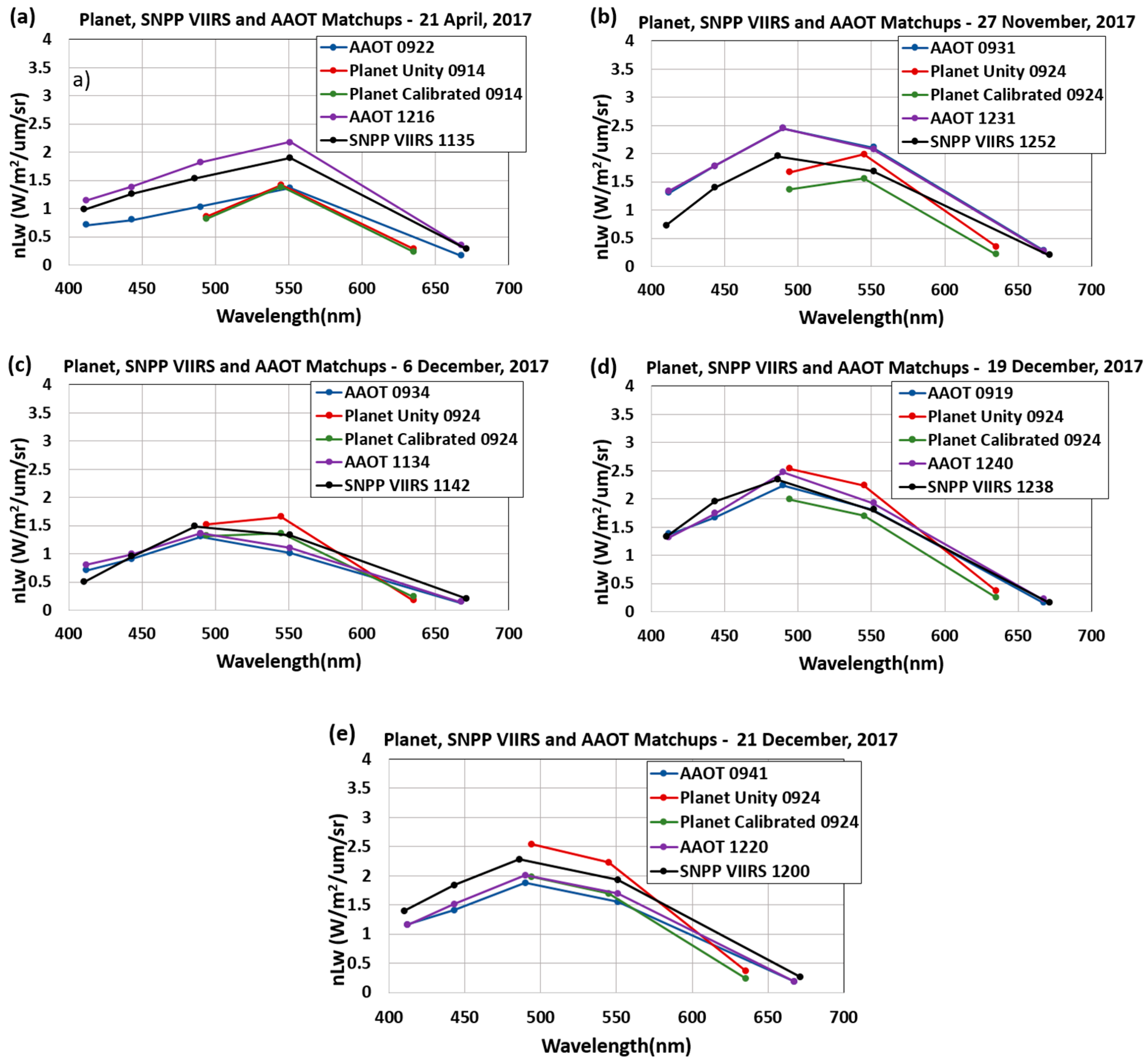
Each of these scenes was processed with APS using unity and calibrated gains to generate $n{L}_w$ measurements for each Dove wavelength. In addition, the VIIRS scene for each of these days was processed to generate the corresponding $n{L}_w$ for comparison. The $n{L}_w$ measurements from the AAOT sensor were acquired from AERONET-OC. The comparison graphs of the $n{L}_w$ values for these sensors are shown in Figure 2. The AAOT $n{L}_w$ measurement closest to the Dove acquisition time is shown in blue, while the Dove $n{L}_w$ measurements for the unity and calibrated gain processing are shown in red and green, respectively. The AAOT $n{L}_w$ measurement closest to the VIIRS acquisition time is shown in purple, while the VIIRS $n{L}_w$ measurement is shown in black.

The graphs show mixed results between using the unity and calibrated gains. There is little difference between the unity and calibrated results on 21 April 2017 and they both match the AAOT measurement at the corresponding time reasonably well. The unity gain results are closer to the AAOT measurements on 27 November 2017, while the calibrated gain results are closer to the corresponding AAOT measurements on 6 December 2017, 19 December 2017, and 21 December 2017.The VIIRS results track well spectrally with the AAOT measurements taken at the time closest to the VIIRS acquisition. Even though there is a 2–3 h difference between the Dove and VIIRS acquisitions, both Dove sensors’ unity and calibrated gain results match well with the VIIRS measurements.

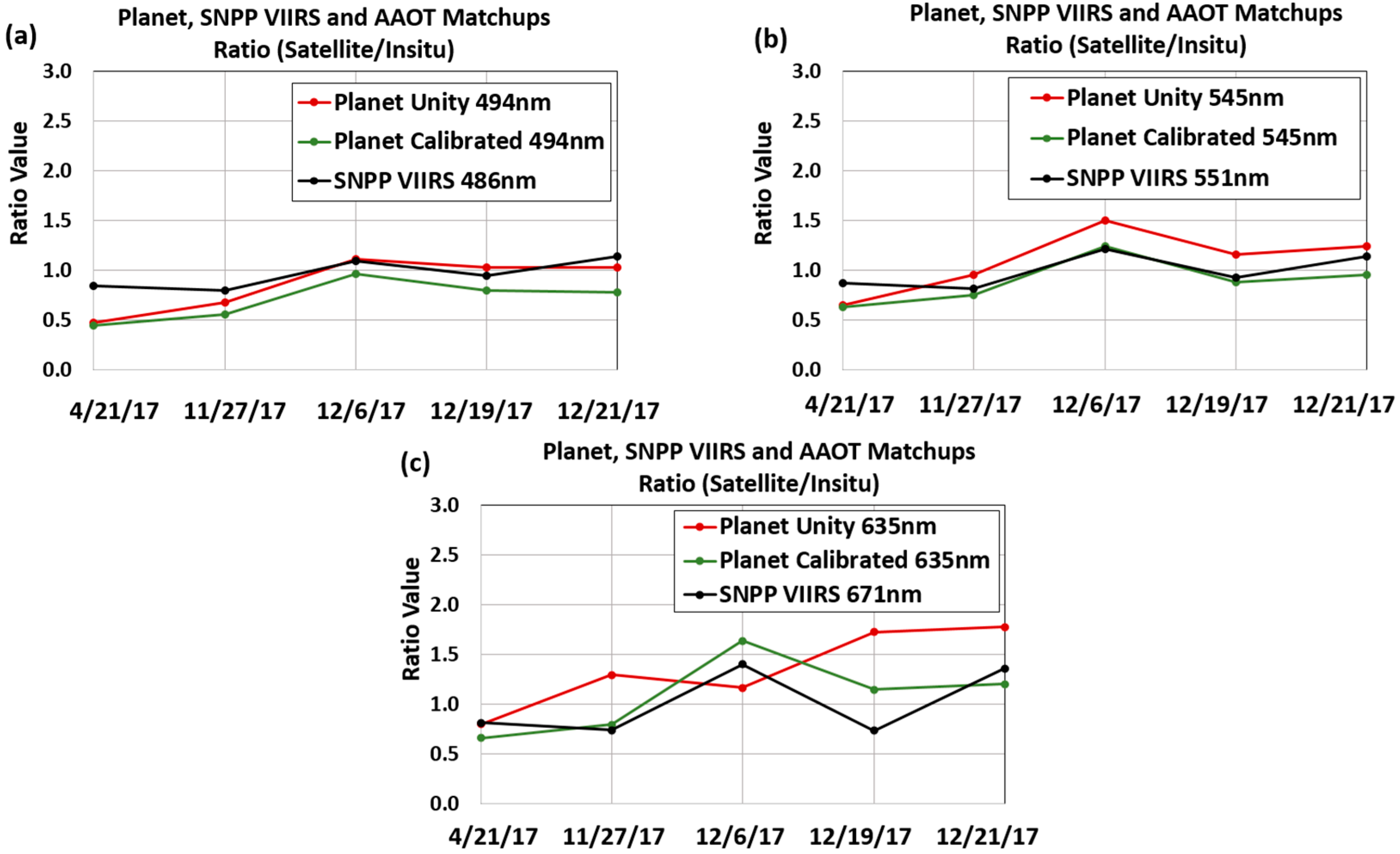
This comparison of the Dove, VIIRS, and AAOT sensors is further detailed in Figure 3. The ratio between the Dove and AAOT as well as VIIRS and AAOT are shown. Using the in situ AAOT $n{L}_w$ as a truth value, these ratios will be 1.0 when the satellite sensors $n{L}_w$ equals the in situ measurement. The VIIRS and corresponding AAOT measurements are close to 1.0. For the 494 nm wavelength, the unity gain Dove results are closer to 1.0. However, for the 545 nm wavelength, the calibrated gain Dove results are closer to 1.0. The $n{L}_w$ value for the 635 nm wavelength is typically small and inherits noise, except for in turbid or sediment-laden waters. Therefore, even a small error can make the ratio jump well above or sink well below 1.0. Despite this, the VIIRS-to-AAOT $n{L}_w$ ratio is still relatively close to 1.0. The calibrated gain Dove results are more consistently closer to 1.0 than the unity gain Dove results and are also closer to the VIIRS ratio results.

The specific values for these relationships are shown in

Table 7. Ratio values between satellite sensors and AAOT in situ sensor.

	$\mathbf{VIIRS} \mathit{n}{\mathit{L}}_{\mathit{w}}$$/\mathbf{AAOT} \mathit{n}{\mathit{L}}_{\mathit{w}}$	$\mathbf{Unity} \mathbf{Planet} \mathit{n}{\mathit{L}}_{\mathit{w}}$$/\mathbf{AAOT} \mathit{n}{\mathit{L}}_{\mathit{w}}$	$\mathbf{Calibrated} \mathbf{Planet} \mathit{n}{\mathit{L}}_{\mathit{w}}$$/\mathbf{AAOT} \mathit{n}{\mathit{L}}_{\mathit{w}}$
AAOT (490 nm)	486 nm	494 nm	494 nm
21 April 2017	0.847	0.473	0.451
27 November 2017	0.797	0.679	0.559
6 December 2017	1.092	1.116	0.968
19 December 2017	0.944	1.026	0.803
21 December 2017	1.139	1.033	0.781
Average	0.964	0.865	0.712
AAOT (551 nm)	551 nm	545 nm	545 nm
21 April 2017	0.873	0.647	0.636
27 November 2017	0.813	0.954	0.748
6 December 2017	1.211	1.503	1.243
19 December 2017	0.932	1.158	0.882
21 December 2017	1.138	1.246	0.951
Average	0.993	1.102	0.892
AAOT (667 nm)	671 nm	635 nm	635 nm
21 April 2017	0.815	0.802	0.662
27 November 2017	0.740	1.298	0.796
6 December 2017	1.402	1.166	1.637
19 December 2017	0.735	1.728	1.150
21 December 2017	1.361	1.777	1.204
Average	1.010	1.354	1.090

. The average rows in these tables show that, over these 5 days, the unity gain Dove results are slightly better when computing the 494 $n{L}_w$, while the calibrated gain Dove results are better for the $n{L}_w$ at the 545 and 635 nm wavelengths. The average VIIRS-to-AAOT $n{L}_w$ ratio is 0.964 for 486 nm, 0.993 for 551 nm, and 1.01 for 671 nm, indicating that the VIIRS sensor is well calibrated and therefore justified to be used as a validation benchmark.

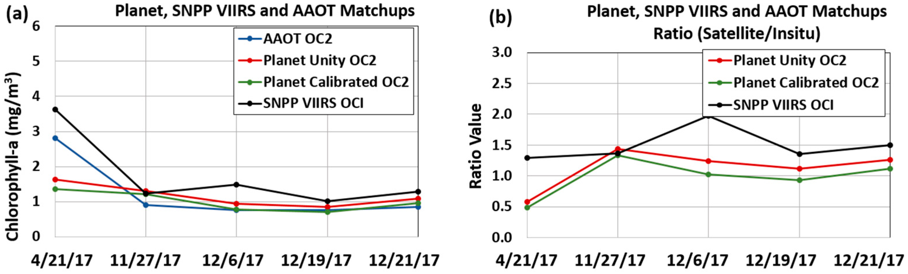
Reasonably accurate $n{L}_w$ can be generated from the Dove sensors, whether using the unity or calibrated gains. Both the $n{L}_w$ and remote sensing reflectance ($R_{\mathrm{r}\mathrm{s}}$), which can be derived from $n{L}_w$, are used to generate a variety of bio-optical ocean color products. The APS chlorophyll product was also generated after atmospheric correction, and the AAOT chlorophyll values were obtained from AERONET-OC. This comparison of the Dove, VIIRS, and AAOT sensors’ chlorophyll measurements is further detailed in Figure 4, with the calibrated Dove consistently closest to 1.0 in Figure 4b.

The values of the satellite-to-AAOT sensor ratios are shown in

Table 8. Ratios of satellite sensor chlorophyll to AAOT in situ sensor chlorophyll.

	VIIRS Chlorophyll/AAOT Chlorophyll	Unity Planet Chlorophyll/AAOT Chlorophyll	Calibrated Planet Chlorophyll/AAOT Chlorophyll
21 April 2017	1.293	0.579	0.486
27 November 2017	1.360	1.434	1.337
6 December 2017	1.971	1.238	1.024
19 December 2017	1.358	1.120	0.934
21 December 2017	1.496	1.260	1.117
Average	1.495	1.126	0.980

. The averages of these ratios show that the calibrated Dove results are closest to 1.0 and even outperform the VIIRS sensor results. The expectation is that, due to being a well-calibrated sensor, the VIIRS sensor should outperform the Dove sensor. However, it is possible that if the sample size was expanded to more dates, the average ratio of the VIIRS-derived chlorophyll values to those of AAOT might be closer to 1.0. In addition, the Dove and VIIRS scenes were acquired at an average of 3 h apart, which could result in haze or atmospheric contamination influencing the VIIRS chlorophyll value. Also, the VIIRS 750 m resolution is larger than the resolution of the AAOT radiometer, allowing for variations in data within the VIIRS pixel. Regardless, the calibrated Dove results provide estimates of the AAOT chlorophyll well.

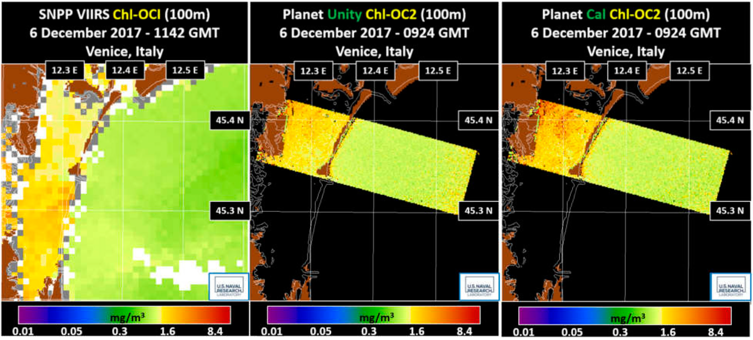
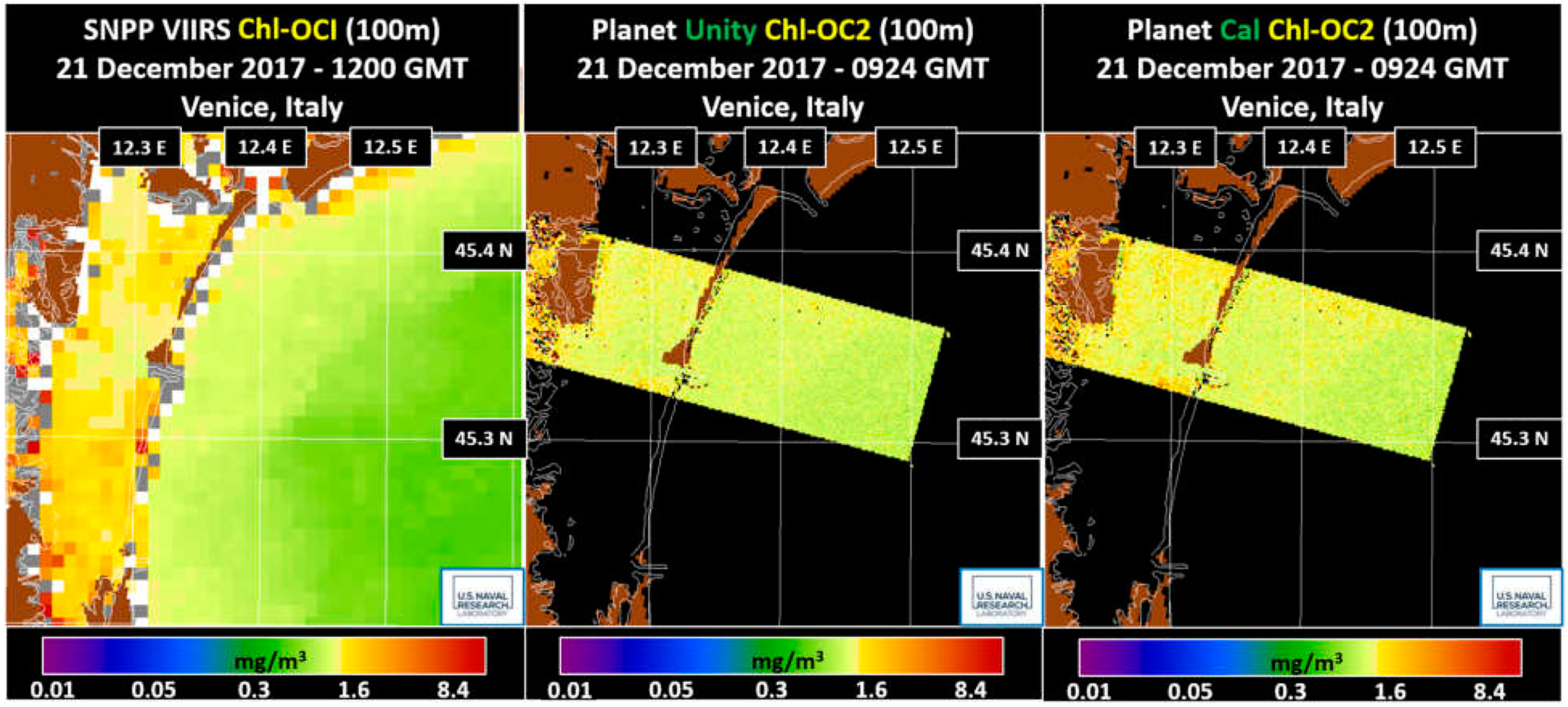
The 6 December 2017 and 21 December 2017 Dove scenes were selected to highlight the comparison of their products to the VIIRS products from coincident scenes. Images for several products were generated and compared. The comparisons highlight the utility of deriving bio-optical products from Dove sensor data for the analysis of ocean phenomena. VIIRS is a polar-orbiting Earth-observing sensor that has been well calibrated with MOBY and other sensors [27]. The sequence of figures displays the VIIRS version of the highlighted product on the left, with the version for the unity gain Dove scene in the middle, and the version for the calibrated gain Dove scene on the right.

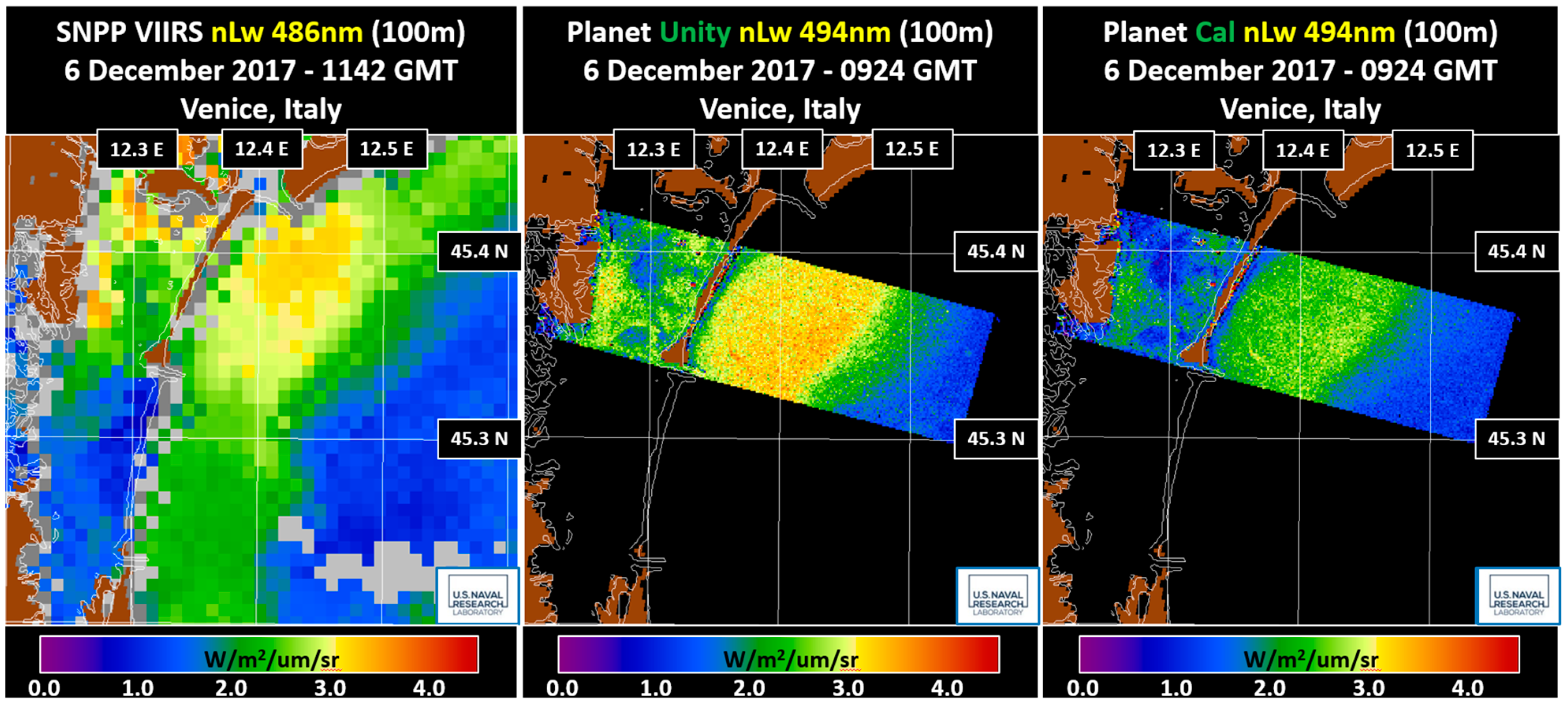
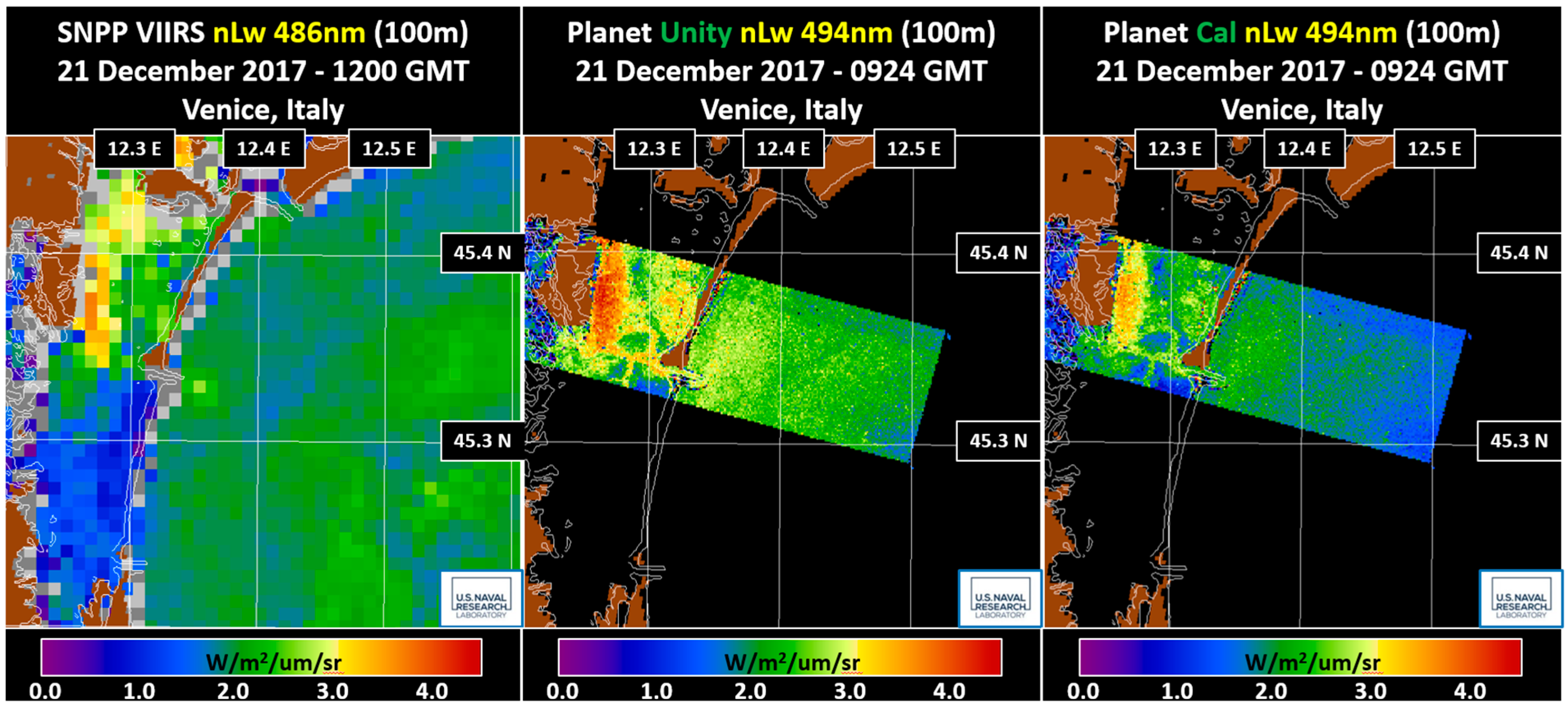
The VIIRS $n{L}_w$ values at 486 nm and Dove $n{L}_w$ at 494 nm wavelength bands for 6 December 2017 and 21 December 2017 are shown in Figure 5 and Figure 6. As with the following figures, this is an area in the Adriatic Sea just off the coast of Venice, Italy. The VIIRS and Dove images were resampled to 100 m resolution to perform this visual comparison. However, the native Dove resolution is about 3 m, so with the resampling to 100 m, much of the detail in the Dove imagery simply cannot be shown in the figures. Showing the imagery at the native 3 m resolution requires graphics too large for display.

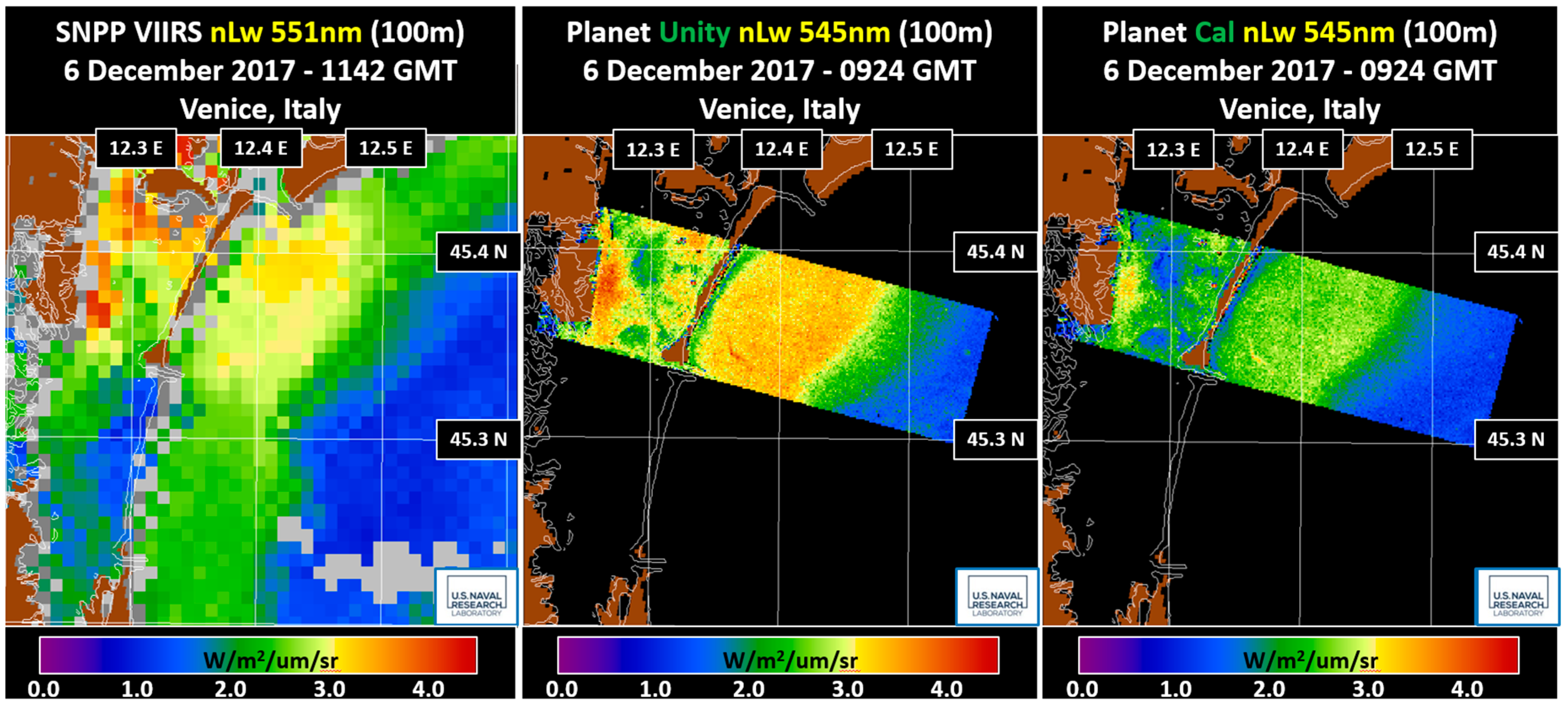
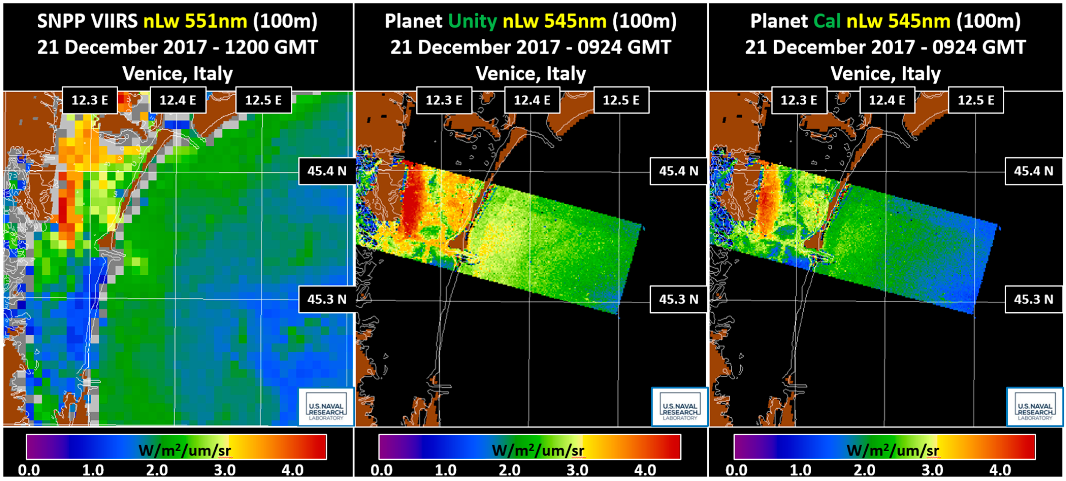
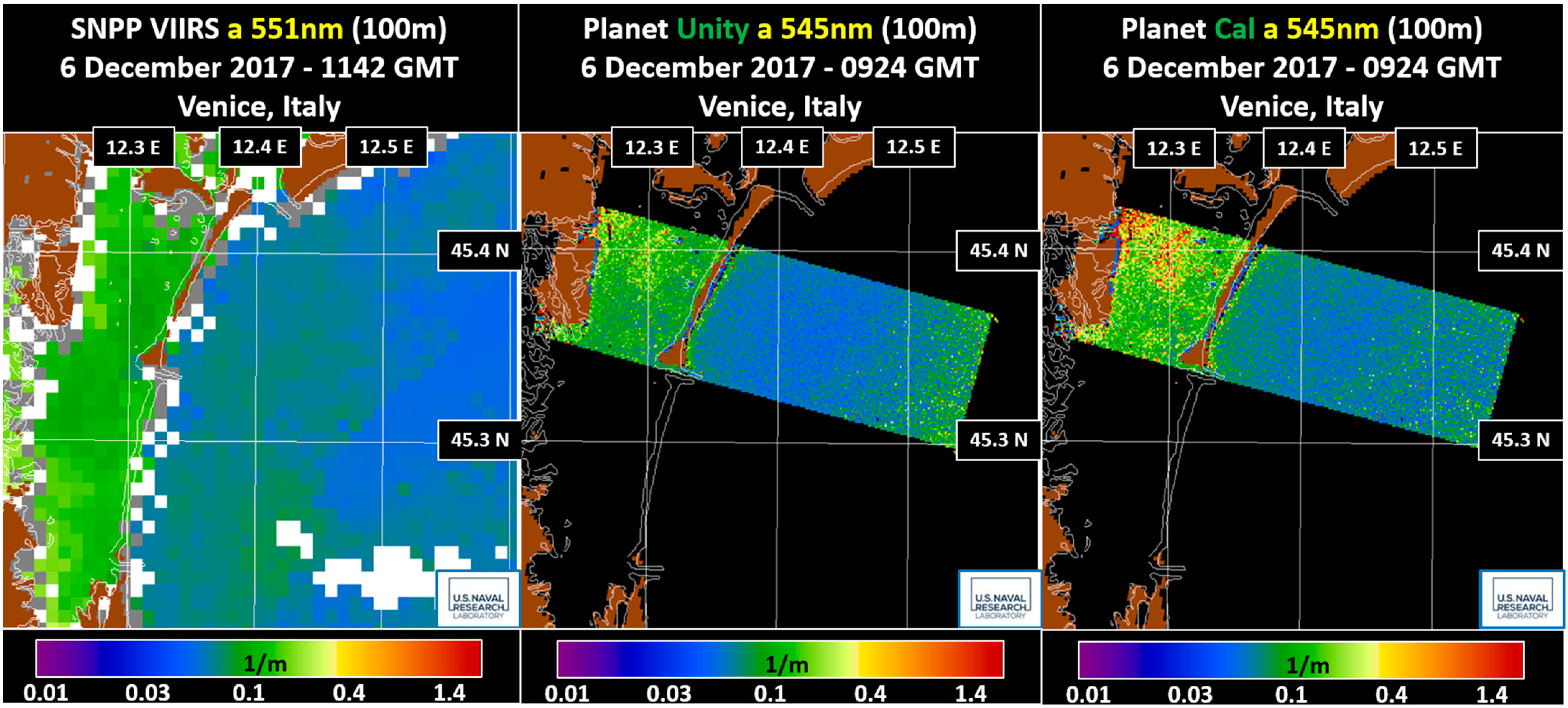
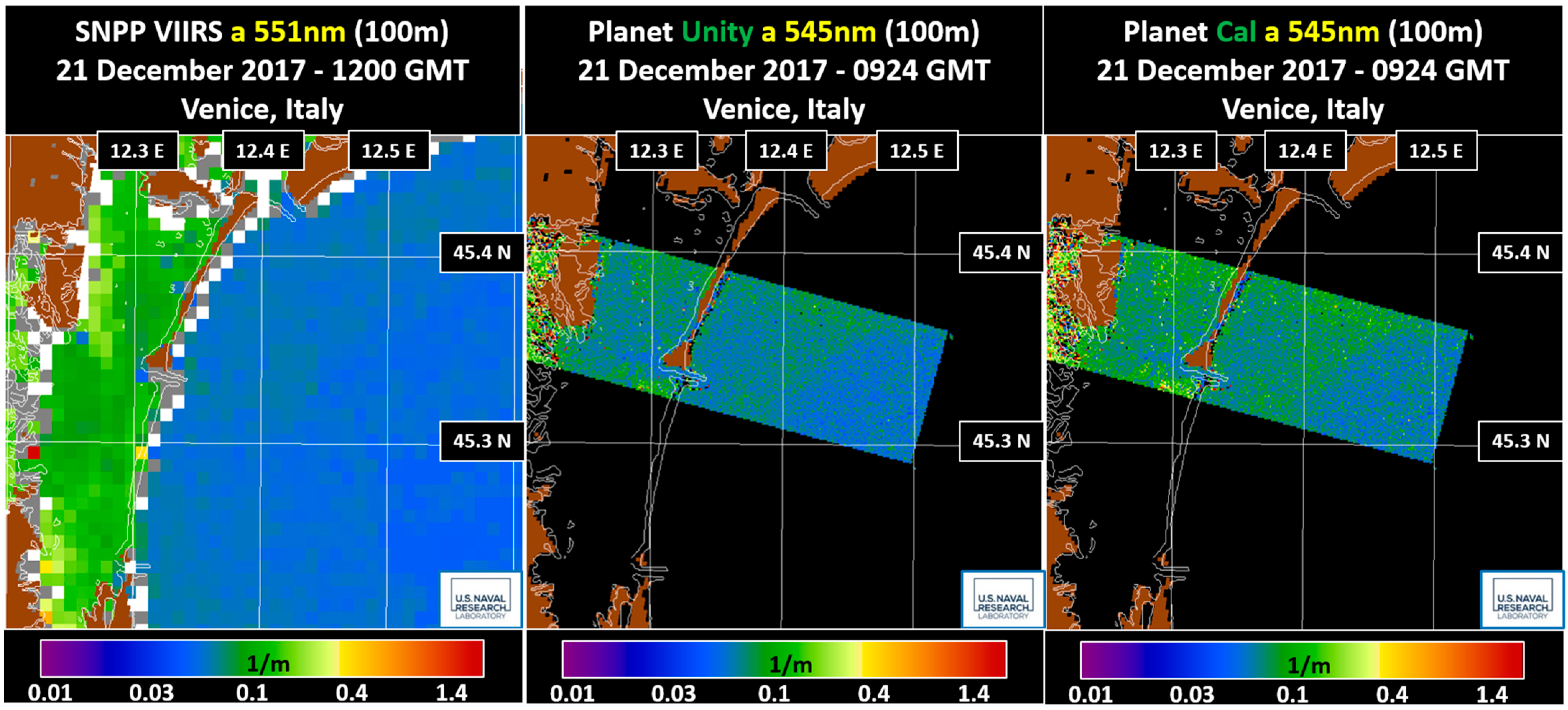
The comparison of the VIIRS $n{L}_w$ at 551 nm, unity gain Dove $n{L}_w$ at 545 nm and calibrated gain Dove $n{L}_w$ at 545 nm for 6 December 2017 and 21 December 2017 is shown in Figure 7 and Figure 8. Like the previous figure, the duplication of VIIRS data and the aggregation of the Dove data used for the resampling leave the VIIRS imagery as coarse blocks, while details of the features in the Venetian Lagoon are seen in the Dove images. The red dots in the Dove images just south of Venice are the small islands of Sacca Sessola, Isola San Spiritu, and Poveglia. These islands are not included in the land mask, which is shaded in brown, and as a result, atmospheric correction failure occurred when they were processed as water pixels. Each of these islands is less than 750 m across, so each is completely consumed within one pixel of the 750 m VIIRS image. However, they are visible in the Dove images, even with the native 3 m data being aggregated to 100 m for display. Even with this aggregation, the features of the deeper channels just inside the Malamocco inlet and elsewhere in the Venetian Lagoon are clearly delineated.

The VIIRS 671 nm wavelength band is the closest VIIRS band to the Dove 635 nm wavelength band. Although these comparisons were shown in the ratio products previously, the imagery of these $n{L}_w$ products were not shown due to the 36 nm difference in wavelength centers. However, the VIIRS and Dove chlorophyll products for 6 December 2017 and 21 December 2017 are shown in Figure 9 and Figure 10.

The VIIRS $K_{\mathrm{d}}$ at 551 nm along with the Dove $K_{\mathrm{d}}$ at 545 nm for 6 December 2017 and 21 December 2017 are shown in Figure 11 and Figure 12.

The comparison of the VIIRS and Dove total absorption ($a$) products for 6 December 2017 and 21 December 2017 are shown in Figure 13 and Figure 14.

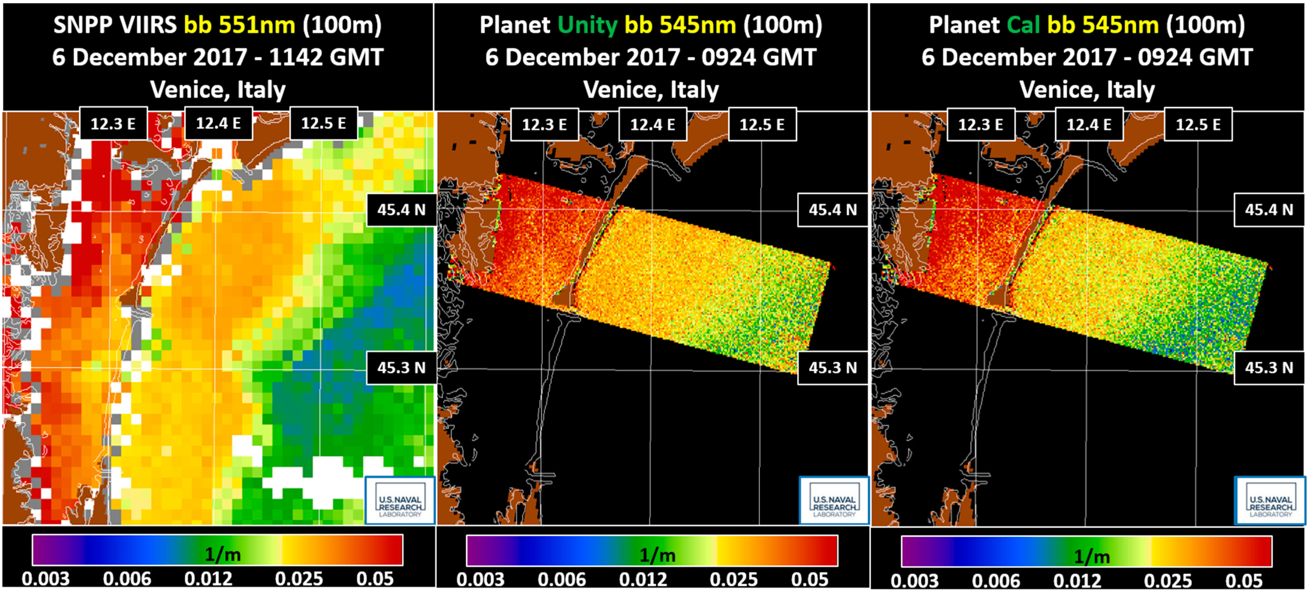
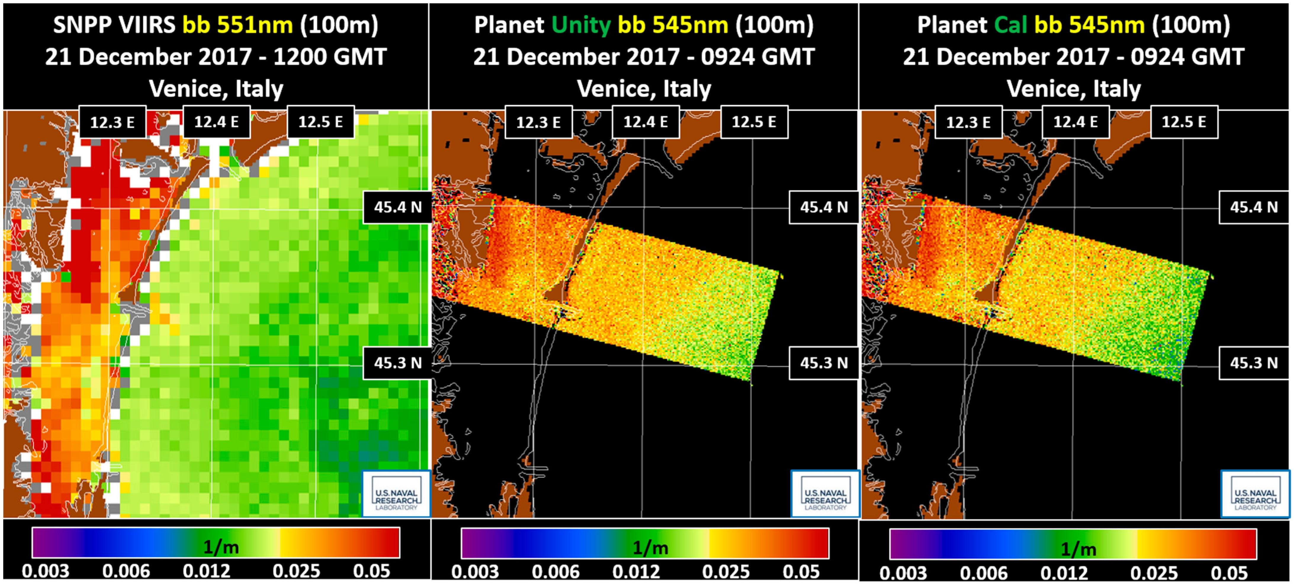
The comparison of the VIIRS and Dove total backscattering ($bb$) products at 551 and 545 nm for 6 December 2017 and 21 December 2017 are shown in Figure 15 and Figure 16.

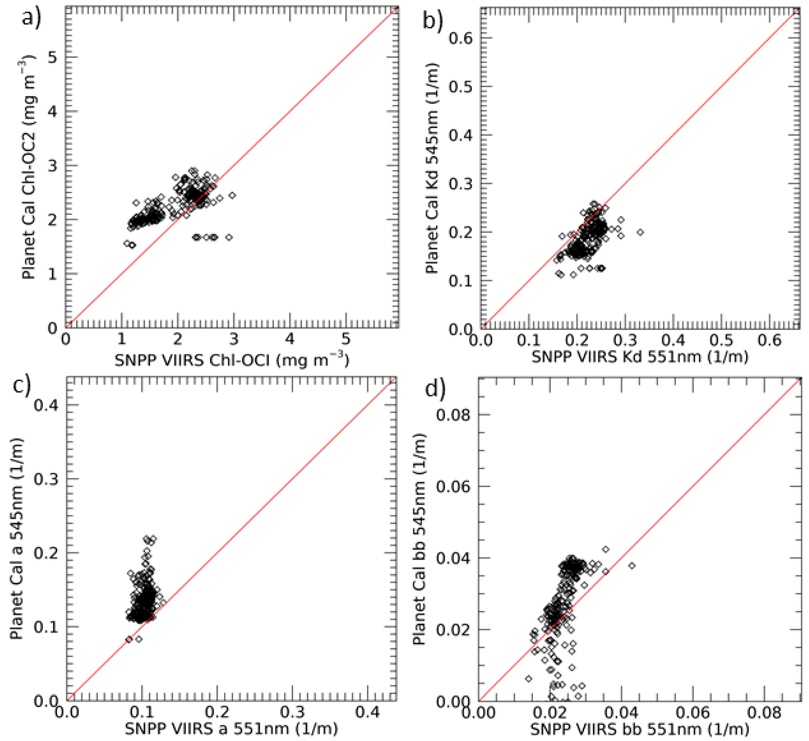
Scatter plots for the VIIRS and calibrated Dove IOP datasets were performed. Since the VIIRS pixels in the Venetian Lagoon were contaminated by a mixture of water and land, the region of interest for the scatter plots was the masked area off-shore that was common to both the VIIRS and Dove scenes. The scatter plots between the VIIRS and calibrated Dove datasets for chlorophyll, diffuse attenuation, absorption, and backscatter at 551 nm wavelength are shown in Figure 17. The scatter plots between the VIIRS and unity Dove datasets are very similar and therefore are not shown here. To facilitate these scatter plots, the VIIRS and Dove images for 21 December 2017were both mapped to the VIIRS sensor spatial resolution of 750 meters.

4. Discussion

Planet has developed nanosatellite Dove sensors that fly in flock formations. Individual or mosaicked scenes are uniquely poised to provide high-resolution information on water properties within coastal and open-ocean scenes. Planet product descriptions for the Dove sensors elaborate on activity to intercalibrate the sensors for scientific investigation [32]. Vicarious calibration is performed on satellite-based Earth-observing sensors to correct for the impact of launch and the harsh space environment that these sensors experience, which cause degradation and drift over time, in addition to the added error due to the atmospheric correction during the L1B to L2 processing. Even if the sensors are well calibrated and record the top of the atmosphere radiance accurately, only having one near infra-red (NIR) wavelength band impacts their ability to gain the full advantage of the atmospheric correction over ocean targets developed by Gordon and Wang [9]. In addition to the 819 nm wavelength used for the longer wavelength band in the Gordon and Wang atmospheric correction process, the 635 nm wavelength band was used as the shorter wavelength band. Even though this wavelength is not a second NIR wavelength and is near the red-edge section of the wavelength, the process was performed to evaluate if a reasonable atmospheric correction could be performed. Bio-optical ocean color products using this approach were generated using APS and compared with products from the well-calibrated VIIRS sensor to validate the Dove sensors for use in ocean research. Since the atmospheric correction process reduces the $n{L}_w$ value of the shorter wavelength band used in atmospheric correction to 0.0, the 635 nm wavelength band was duplicated, allowing for the duplicated band to participate in the atmospheric correction process and the original band to represent the $n{L}_w$ value at the visible 635 nm wavelength.

The Dove data for this analysis were purchased from Planet. These included scenes over the MOBY calibration and validation sensors and AERONET-OC locations. Vicarious calibration and initial validation were performed using the MOBY data and additionally validated with the AAOT AERONET-OC sensor in the Adriatic Sea off the coast of Venice, Italy. Five scenes were used to generate calibrated gains from the vicarious calibration process. Ideally, there should be more matches for calibration; however, many scenes were impacted by clouds or haze. The five scenes selected represented the best collection of cloud-free scenes over the MOBY sensor. The generated calibration gain sets were 0.9649, 0.9554, 0.9767, 0.94990, and 1.0 for the 494, 545, 635 (visible), 635 (for atmospheric correction), and 819 nm wavelengths, respectively.

Table 6 shows the improvement when using the calibrated gains for the scenes processed with the MOBY sensor. This shows the ratio between the unity and calibrated $n{L}_w$. Ideally, the ratio of the satellite-to-in situ measurement is 1.0. The “Unity” and “Calibrated” rows show the $n{L}_w$ ratio of the Dove to MOBY sensor for each wavelength. The “Calibrated” row shows ratio values near 1.0 for each wavelength, while the “Difference” row shows the difference between the “Unity” and “Calibrated” ratios consistently indicating improvement after calibration.

However, this improvement is computed with data from the dates used to compute the gains. Dove scenes over the AAOT AERONET-OC platform were used to validate products generated from Dove data using a separate test set that did not participate in computing the calibration gains. Therefore, five Dove scenes over the AAOT platform were processed with both unity and calibrated gains. This allowed us to use in situ data from the AAOT sensor in the Adriatic Sea in the validation of calibrated gains that were computed using in situ data from waters near Hawaii, almost 13,000 km away.

In addition, VIIRS data for these dates were also downloaded and processed for comparison. Table 2 shows the dates and times of the Dove, AAOT, and VIIRS acquisitions. The time difference between the Dove and AAOT measurements was less than 20 min on all the dates. The time difference between the VIIRS and AAOT measurements was less than 45 min on all the dates. Although these time differences are not large, the acquisition times of the Dove and VIIRS sensors are up to 3.5 hours apart.

The Planet Dove, VIIRS, and AAOT graphs in Figure 2 show that the unity and calibrated Dove $n{L}_w$ values, represented with the red and green lines, both correspond reasonably well to the AAOT $n{L}_w$ measurements represented in the blue line. The VIIRS and corresponding AAOT measurements recorded nearer to the VIIRS acquisition time also correspond reasonably well. Even with the time difference between the VIIRS and Dove acquisition, the $n{L}_w$ measurements from those sensors correspond well. The errors obtained when assuming the AAOT in situ data to be true are shown in the graphs of Figure 3. These ratios between the satellite-estimated $n{L}_w$ and in situ-measured $n{L}_w$ will be 1.0 if the satellite estimate is equal to the in situ measurement. The graphs show that the ratios of VIIRS 486 nm $n{L}_w$ estimates to the AAOT 490 nm $n{L}_w$ measurements hover around 1.0. The ratios of the unity and calibrated Dove 494 nm $n{L}_w$ estimates to AAOT 490 nm $n{L}_w$ measurements are both low for 21 April 2017 and 27 November 2017. However, they approach 1.0 for dates 6 December 2017, 19 December 2017, and 21 December 2017. The results for the two gain sets show the unity gain results are better than the calibration results for the 494 nm wavelength. However, the $n{L}_w$ for the 545 and 635 nm wavelength bands are estimated better with the calibrated gain set.

These observations are strengthened by the results of the quantification of the ratios in Table 7. The average of the ratios over the 5 days for the Dove 494 nm wavelength is 0.87 for the unity gain results and 0.71 for the calibrated gain results. The average of the ratios for the Dove 545 nm wavelength is 1.10 for the unity gain results and 0.89 for the calibrated gain results. So, the calibrated gain results underestimate the AAOT $n{L}_w$ almost as much as the unity gains overestimate the AAOT $n{L}_w$. The average of the ratios for the Dove 635 nm wavelength is 1.354 for the unity gain results and 1.09 for the calibrated gain results.

Chlorophyll is an important measurement as it relates to primary productivity. Accurate chlorophyll estimation is important to characterize the distribution of chlorophyll in the Dove scenes. The chlorophyll algorithm is based on $n{L}_w$ values in the blue and green wavelengths. A comparison of the Dove, VIIRS, and AAOT chlorophyll measurements is shown in Figure 4a. Except for 4/21/17, these estimates match very well over the 5-day period. Similar validation ratios as those shown for the individual $n{L}_w$ wavelength estimates are shown for chlorophyll in Figure 4b. The Dove ratios are low for 21 April 2017and then slightly high for the remaining days, with the calibrated gain results performing better than the unity gain results. These trends are further reinforced in Table 8 with the average of the validation ratios being 0.98 for the calibrated results and 1.126 for the unity gain results.

A series of image products were generated from two Dove scenes using both gain sets and the coincident VIIRS of $n{L}_w$, chlorophyll, and IOP products for those days were also generated. The image comparisons of $n{L}_w$ products at the VIIRS 486 nm and Dove 494 nm wavelengths, using both unity and calibrated gains, for 6 December 2017 and 21 December 2017 are shown in Figure 5 and Figure 6. These figures show that the values obtained with the Dove product based on unity gain match better, at least from the standpoint of the orange and yellow colors in the off-shore. However, the Dove product based on calibrated gains does not significantly underestimate the VIIRS values. It should be noted that there is an 8 nm difference between the VIIRS and Dove wavelengths in this comparison. Visually, the unity gain Dove 494 nm $n{L}_w$ appears to match more closely to the VIIRS 486 nm $n{L}_w$ image for 6 December 2017. However, the calibrated gain version appears to match more closely for 21 December 2017.

The image comparisons of $n{L}_w$ products at the VIIRS 551 nm and Dove 545 nm wavelengths, using both unity and calibrated gains, for 6 December 2017 and 21 December 2017 are shown in Figure 7 and Figure 8. The green, yellow, and orange colors in these figures indicate that the unity gain Dove 545 nm $n{L}_w$ overestimates the VIIRS 551 nm $n{L}_w$ image for 6 December 2017. The calibrated gain Dove 545 nm $n{L}_w$ values match the VIIRS 551 nm $n{L}_w$ well, even though it slightly underestimates the VIIRS values.

The image comparisons between the VIIRS and Dove chlorophyll products for both the unity and calibrated gains on for 6 December 2017 and 21 December 2017 are shown in Figure 9 and Figure 10. Both the unity and calibrated gain versions match the VIIRS image well, with the calibrated gain matching more closely.

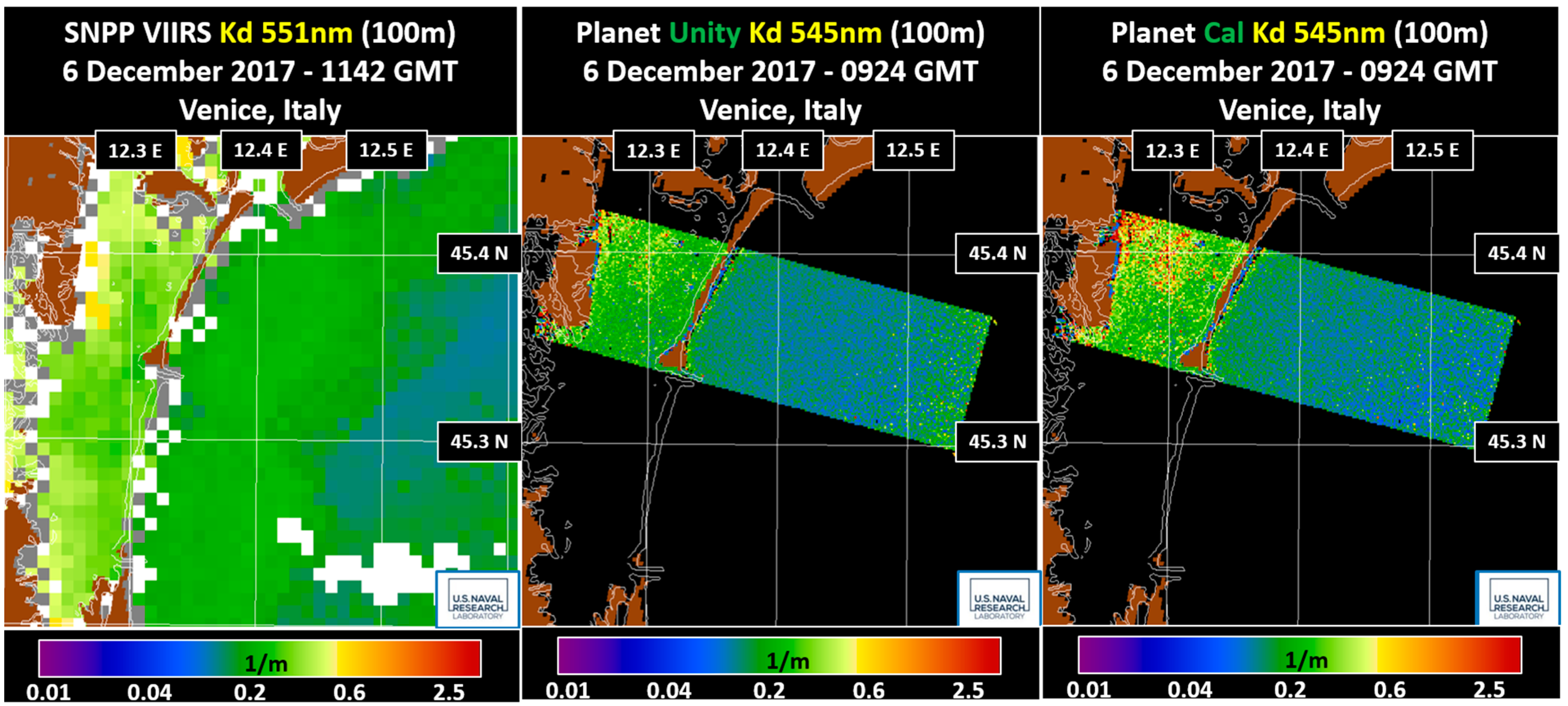
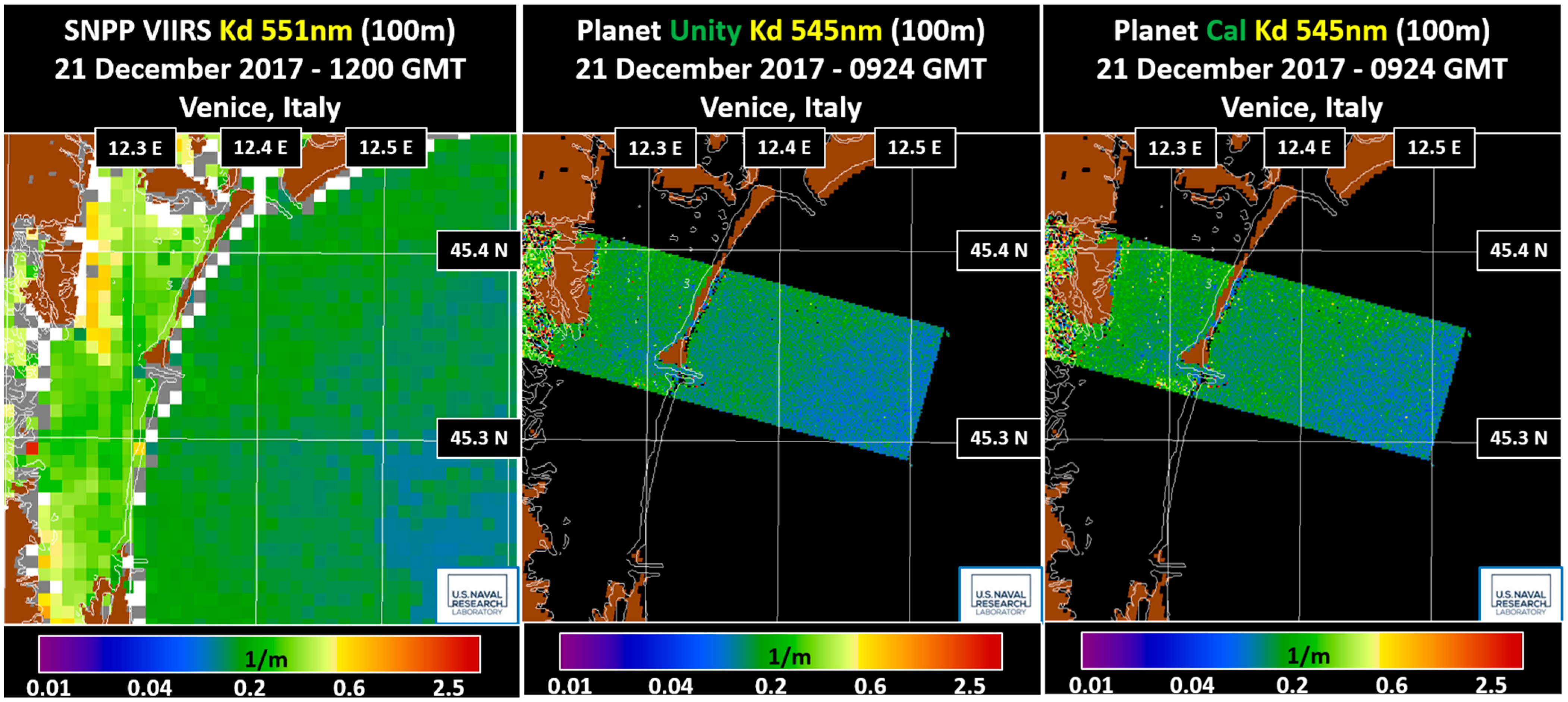
The ability to compute IOPs from remotely sensed water-leaving radiance data allows for the analysis of the properties of coastal and open waters. Due to limited wavelength information, data from the Dove sensors cannot be used in the QAA algorithm to compute IOPs [28]. However, empirical methods of computing IOPs have been developed [29,31]. Since the Dove sensors lack the wavelength bands to perform the QAA algorithm, simple one- and two-band empirical methods were used to compute IOP products for the Dove scenes [30]. Several IOP products from VIIRS and Dove were computed, including VIIRS diffuse attenuation, absorption, and backscatter at 551 nm, as well as Dove diffuse attenuation, absorption, and backscatter at 545 nm. The VIIRS products were generated using the QAA algorithm available in APS. The images of these products are shown in Figure 11 through Figure 16, with the calibrated results performing better over the two dates.

Both gain sets in Figure 11 and Figure 12 generated $K_{\mathrm{d}}$ products that matched VIIRS well. This shows higher attenuation within the muddy or bottom-contaminated waters of the Venetian Lagoon. The delineation of the channels is not as pronounced as with the $n{L}_w$ products since the attenuation is more uniform across the waters of the lagoon.

Although only absorption at 545 nm is shown in Figure 13 and Figure 14, further partitioning of this IOP can provide information on the water’s constituent components of phytoplankton, colored dissolved organic matter (CDOM), and detritus, which provides details of the water composition in the scene [33]. The waters in the lagoon estuary have higher values of absorption, reflecting the integrated concentrations of phytoplankton, CDOM, and detritus.

The analysis of backscatter at 551 and 545 nm in Figure 15 and Figure 16 provides information about sediment loading and movement in the coastal region. It also provides insight into detritus, particulate organic carbon (POC), and particulate inorganic carbon (PIC) biomass.

The derivation of the $K_{\mathrm{d}}$, $a$, and $bb$ estimates from the Dove scenes provide insight into the Venetian Lagoon and coastal waters. The Dove $K_{\mathrm{d}}$ products for both gain sets show a decrease in $K_{\mathrm{d}}$ measurement in the Venetian Lagoon, but an increase off-shore in the Adriatic Sea from 6 December 2017 and 21 December 2017. The diffuse attenuation coefficient is a water property derived through IOPs related to the impact of light penetration and attenuation on light availability in aquatic systems. It contributes to the characterization of the heat transfer in the upper layer of the ocean [34,35,36,37] and also to biological processes such as phytoplankton photosynthesis in the ocean euphotic zone [38,39]. The optical backscatter IOP is correlated with the concentration and microphysical characteristics of water column constituents such as chlorophyll [40], detrital/particulate biomass [41], and particulate organic carbon (POC) [42,43] and particulate inorganic carbon (PIC) [44].

The scatter plots shown in Figure 17a show a reasonable match along the red one-to-one line between the VIIRS and calibrated Dove estimated chlorophyll values for 21 December 2017. For the Dove sensor, this chlorophyll is used as input into the empirical IOP algorithms. The remaining scatter plots in Figure 17 between VIIRS and the calibrated Dove for diffuse attenuation, absorption, and backscatter represent a reasonable match between the VIIRS and Dove IOPs. The computed chlorophyll from APS provides IOP estimations that match VIIRS reasonably well. Therefore, the empirical algorithms represent a valid approach for computing IOPs for the Dove sensor.

5. Conclusions

The limitations of the presented methodologies include the reduced sample size in performing vicarious calibration, the challenges posed by the red wavelength band used for atmospheric correction, and to some extent the limited datasets available for the analysis. Future improvements include the increased wavelength bands that are expected on upcoming Planet sensors. Additional data can provide opportunities to increase the number of scenes used for both fine-tuning the calibration and expanding validation. One benefit of the Dove and future Planet nanosatellite sensors is their high spatial resolution for exploring estuaries and rivers. The methodologies presented in this study show that useful apparent optical properties in the form of water-leaving radiance and inherent optical properties in the form of diffuse attenuation, absorption, and backscatter can be generated from the Dove sensors.

Regarding the limitations, data for the vicarious calibration and validation were acquired from Planet via a data purchase agreement. This allowed us to obtain data over MOBY and AAOT. However, it did not provide a dataset as extensive as is typically used for the vicarious calibration of other polar-orbiting sensors. In addition, visual and analytical approaches eliminated some scenes from use in calibration, which were contaminated by haze, clouds, or other atmospheric effects, so only data from clear days were used. This reduced the available scenes for vicarious calibration further. Although sample sizes for vicarious calibration of polar-orbiting sensors, such as VIIRS, do have a larger sample size in the calibration process, similar scene-screening methods are performed for these sensors as well. In this sense, even though the sample size used in this calibration was a reduced sample of only five dates, the calibration process proceeded as traditionally performed to fine-tune the sensor gains so that the Dove sensor could generate useful results. For continued work in the future, additional scenes could be used to increase the sample size of the vicarious calibration and further fine-tune the sensor gains. Along these same lines, although a collection of Planet Dove data was purchased for the evaluation, there were limited Dove scenes over the AAOT in situ location for validation. Therefore, for demonstration, Dove scenes acquired on the five dates were compared with VIIRS.

This vicarious calibration of the Dove sensors was performed not only to compute sensor gains for calibration but also to assess the performance of atmospheric correction using Dove data. Limitations in wavelength bands led to the inclusion of a red and NIR band to be used in the atmospheric correction process for selecting an aerosol model, as opposed to the use of two NIR bands that are available in most ocean color sensors. The Gordon and Wang atmospheric correction algorithm uses two NIR bands: one called the “short” NIR and the other the “long” NIR band [9]. The impact of using the red (635 nm) band as the “short” NIR band in atmospheric correction instead of two NIR bands is the expectation of what the residual signal in the “short” NIR band represents. The assumption is that it represents additional light scattering that occurs due to aerosol composition. By using the red band in this methodology, the signal of remaining radiance at this wavelength is mistakenly interpreted as aerosol radiance and not water-leaving radiance. This guides the algorithm to remove values interpreted as the aerosol radiance from the other wavelength bands. Since this is the red wavelength, the impact of this misrepresentation will be more evident in sediment-laden, turbid waters that have a red or brown color.

Despite these limitations, quality ocean color data were generated over the Venetian Lagoon. The use of the red band in atmospheric correction did not prevent the computation of useful ocean color data. The chlorophyll values computed using the water-leaving radiance matched the chlorophyll values measured at the AAOT site location for the sample of 5 days. The scatter plot of Dove IOPs compared well with the collocated VIIRS IOPs. This demonstrates the utility of Dove data.

One point of interest concerning the Dove imagery, especially in the coastal region, is the usefulness of the improved spatial resolution. The presented images for both VIIRS and Dove were resampled to a 100-meter resolution. Therefore, the 750-meter VIIRS resolution was duplicated for the corresponding 100-meter cells in the resampled image, while the 3-meter Dove resolution data were subsampled. Even with the Dove subsampling, the variation in $n{L}_w$ across channel depths was evident in the areas around the marshes of the Venetian Lagoon just inside the Malamocco inlet. The 750-meter VIIRS resolution results in land contamination for the image pixels in near-shore areas. This results in higher measurements in $n{L}_w$, which affects the derived product values. However, the Dove scenes, with their higher spatial resolution, provided feature detail and delineation in the lagoon’s in-shore waters.

Several hundred Dove sensors have been launched. Follow-on Super-Dove sensors are also being launched that include additional wavelength bands in the visible and at the red edge. This analysis shows that the Dove sensors are well calibrated and traditional methods can be employed with Dove scene data to perform in-orbit vicarious calibration and generate bio-optical ocean color products. The 3-meter spatial resolution of the Dove sensors allows for optical properties in near-shore areas to be computed and analyzed for water quality. The usefulness of the sensors in locations both over in-land estuaries and off-shore waters provides a new capability for high-resolution studies of the ocean.

Coarser-resolution sensors suffer from not only a limited number of image elements that correspond to their spatial resolution in these confined areas but also the blending of water and land pixels for locations along the land–water interface. The results from this analysis show that Planet Dove sensor data can be used to generate remotely sensed ocean color bio-optical products. The high spatial resolution provides the ability to explore bays, estuaries, and rivers in ways that are not possible with the use of sensors with coarser spatial resolution.

References

- Curzi, G.; Modenini, D.; Tortora, P. Large Constellations of Small Satellites: A Survey of Near Future Challenges and Missions. Aerospace 2020, 7, 133. [Google Scholar] [CrossRef]
- Sanad, I.; Vali, Z.; Michelson, D.G. Statistical Classification of Remote Sensing Satellite Constellations. In Proceedings of the 2020 IEEE Aerospace Conference, Big Sky, MT, USA, 7–14 March 2020; pp. 1–15. [Google Scholar]
- Franz, B.A.; Bailey, S.W.; Werdell, P.J.; McClain, C.R. Sensor-independent approach to the vicarious calibration of satellite ocean color radiometry. Appl. Opt. 2007, 46, 5068–5082. [Google Scholar] [CrossRef] [PubMed]
- Bailey, S.W.; Hooker, S.B.; Antoine, D.; Franz, B.A.; Werdell, P.J. Sources and assumptions for the vicarious calibration of ocean color satellite observations. Appl. Opt. 2008, 47, 2035–2045. [Google Scholar] [CrossRef]
- Kwiatkowska, E.J.; Franz, B.A.; Meister, G.; McClain, C.R.; Xiong, X. Cross calibration of ocean-color bands from Moderate Resolution Imaging Spectroradiometer on Terra platform. Appl. Opt. 2008, 47, 6796–6810. [Google Scholar] [CrossRef]
- Wang, M. Rayleigh radiance computations for satellite remote sensing: Accounting for the effect of sensor spectral response function. Opt. Express 2016, 24, 12414–12429. [Google Scholar] [CrossRef]
- Goyens, C.; Jamet, C.; Ruddick, K.G. Spectral relationships for atmospheric correction. II. Improving NASA’s standard and MUMM near infra-red modeling schemes. Opt. Express 2013, 21, 21176–21187. [Google Scholar] [CrossRef] [PubMed]
- McCarthy, S.; Crawford, S.; Wood, C.; Lewis, M.D.; Jolliff, J.K.; Martinolich, P.; Ladner, S.; Lawson, A.; Montes, M. Automated Atmospheric Correction of Nanosatellites Using Coincident Ocean Color Radiometer Data. J. Mar. Sci. Eng. 2023, 11, 660. [Google Scholar] [CrossRef]
- Gordon, H.R.; Wang, M. Retrieval of water-leaving radiance and aerosol optical thickness over the oceans with SeaWiFS: A preliminary algorithm. Appl. Opt. 1994, 33, 443–452. [Google Scholar] [CrossRef] [PubMed]
- Franz, B.; Kwiatkowska, E.; Meister, G.; McClain, C. Moderate Resolution Imaging Spectroradiometer on Terra: Limitations for ocean color applications. J. Appl. Remote Sens. 2008, 2, 023525. [Google Scholar] [CrossRef]
- Carl, F.S.; John, E.C.; Philip, E.A.; Carol, W.; Frank, D.; Hilmer, S. NPOESS VIIRS sensor design overview. In Proceedings of the SPIE, International Symposium on Optical Science and Technology, San Diego, CA, USA, 29 July–3 August 2001; pp. 11–23. [Google Scholar]
- Brown, L.A.; Dash, J.; Lidón, A.L.; Lopez-Baeza, E.; Dransfeld, S. Validation of the Sentinel-3 Ocean and Land Colour Instrument (OLCI) Terrestrial Chlorophyll Index (OTCI): Synergetic Exploitation of the Sentinel-2 Missions. In Proceedings of the IGARSS 2018—2018 IEEE International Geoscience and Remote Sensing Symposium, Valencia, Spain, 22–27 July 2018; pp. 8719–8722. [Google Scholar]
- Ryu, J.-H.; Han, H.-J.; Cho, S.; Park, Y.-J.; Ahn, Y.-H. Overview of geostationary ocean color imager (GOCI) and GOCI data processing system (GDPS). Ocean Sci. J. 2012, 47, 223–233. [Google Scholar] [CrossRef]
- Hiroshi, M. Ocean color estimation by Himawari-8/AHI. In Proceedings of the SPIE, SPIE Asia Pacific Remote Sensing, New Delhi, India, 4–7 April 2016; p. 987810. [Google Scholar]
- Baith, K.; Lindsay, R.; Fu, G.; McClain, C.R. Data analysis system developed for ocean color satellite sensors. Eos Trans. Am. Geophys. Union 2001, 82, 202. [Google Scholar] [CrossRef]
- Gordon, H.R. In-orbit calibration strategy for ocean color sensors. Remote Sens. Environ. 1998, 63, 265–278. [Google Scholar] [CrossRef]
- Davis, M. Relative Spectral Response Curves for Planet Dove Sensors. Available online: https://support.planet.com/hc/en-us/articles/360014290293 (accessed on 31 August 2023).
- Lewis, M.D.; Gould, R.W.; Arnone, R.A.; Lyon, P.E.; Martinolich, P.M.; Vaughan, R.; Lawson, A.; Scardino, T.; Hou, W.; Snyder, W.; et al. The Hyperspectral Imager for the Coastal Ocean (HICO): Sensor and data processing overview. In Proceedings of the OCEANS 2009, Biloxi, MS, USA, 26–29 October 2009; pp. 1–9. [Google Scholar]
- Voss, K.; Leymarie, E.; Flora, S.; Carol Johnson, B.; Gleason, A.; Yarbrough, M.; Feinholz, M.; Houlihan, T. Improved shadow correction for the marine optical buoy, MOBY. Opt. Express 2021, 29, 34411–34426. [Google Scholar] [CrossRef] [PubMed]
- Feinholz, M.E.; Flora, S.J.; Yarbrough, M.A.; Lykke, K.R.; Brown, S.W.; Johnson, B.C.; Clark, D.K. Stray Light Correction of the Marine Optical System. J. Atmos. Ocean. Technol. 2009, 26, 57–73. [Google Scholar] [CrossRef]
- Brown, S.W.; Flora, S.J.; Feinholz, M.E.; Yarbrough, M.A.; Houlihan, T.; Peters, D.; Kim, Y.S.; Mueller, J.L.; Johnson, B.C.; Dennis, K. The Marine Optical BuoY (MOBY) radiometric calibration and uncertainty budget for ocean color satellite sensor vicarious calibration. In Proceedings of the SPIE Remote Sensing, Sensors, Systems, and Next-Generation Satellites XI, Florence, Italy, 17–20 September 2007; p. 6744. [Google Scholar] [CrossRef]
- Wilson, N.; Greenberg, J.; Jumpasut, A.; Arin; Collison, A.; Weichelt, H. Absolute Radiometric Calibration of Planet Dove Satellites, Flocks 2p & 2e. Available online: https://earth.esa.int/eogateway/documents/20142/1305226/Absolute-Radiometric-Calibration-Planet-Dove-Flocks-2p-2e.pdf (accessed on 31 August 2023).
- Collison, A.; Jumpasut, A.; Bourne, H. On-Orbit Radiometric Calibration of the Planet Satellite Fleet. Available online: https://assets.planet.com/docs/radiometric_calibration_white_paper.pdf (accessed on 31 August 2023).
- Zibordi, G.; Mélin, F.; Berthon, J.-F.; Holben, B.; Slutsker, I.; Giles, D.; D’Alimonte, D.; Vandemark, D.; Feng, H.; Schuster, G.; et al. AERONET-OC: A Network for the Validation of Ocean Color Primary Products. J. Atmos. Ocean. Technol. 2009, 26, 1634–1651. [Google Scholar] [CrossRef]
- MéLin, F.; Clerici, M.; Zibordi, G.; Bulgarelli, B. Aerosol variability in the Adriatic Sea from automated optical field measurements and Sea-viewing Wide Field-of-view Sensor (SeaWiFS). J. Geophys. Res. Atmos. 2006, 111, 22201. [Google Scholar] [CrossRef]
- Twardowski, M.S.; Boss, E.; Sullivan, J.M.; Donaghay, P.L. Modeling the spectral shape of absorption by chromophoric dissolved organic matter. Mar. Chem. 2004, 89, 69–88. [Google Scholar] [CrossRef]
- Wang, M.; Shi, W.; Jiang, L.; Liu, X.; Son, S.; Voss, K. Technique for monitoring performance of VIIRS reflective solar bands for ocean color data processing. Opt. Express 2015, 23, 14446–14460. [Google Scholar] [CrossRef] [PubMed]
- Lee, Z.; Carder, K.L.; Arnone, R.A. Deriving inherent optical properties from water color: A multiband quasi-analytical algorithm for optically deep waters. Appl. Opt. 2002, 41, 5755–5772. [Google Scholar] [CrossRef]
- Qiu, Z.; Wu, T.; Su, Y. Retrieval of diffuse attenuation coefficient in the China seas from surface reflectance. Opt. Express 2013, 21, 15287–15297. [Google Scholar] [CrossRef]
- Lee, Z.-P.; Darecki, M.; Carder, K.L.; Davis, C.O.; Stramski, D.; Rhea, W.J. Diffuse attenuation coefficient of downwelling irradiance: An evaluation of remote sensing methods. J. Geophys. Res. Ocean. 2005, 110, C02017. [Google Scholar] [CrossRef]
- Arnone, R.B.; Babin, M.; Barnard, A.H.; Boss, E.; Cannizzaro, J.P.C.; Carder, K.L.; Chen, R.F.; Devred, E.; Doerffer, R.D.; Du, K.; et al. Remote Sensing of Inherent Optical Properties: Fundamentals, Tests of Algorithms and Applications; IOCCG—International Ocean-Colour Coordinating Group: Dartmouth, NS, Canada, 2006. [Google Scholar]
- Frazier, A.E.; Hemingway, B.L. A Technical Review of Planet Smallsat Data: Practical Considerations for Processing and Using PlanetScope Imagery. Remote Sens. 2021, 13, 3930. [Google Scholar] [CrossRef]
- Isada, T.; Abe, H.; Kasai, H.; Nakaoka, M. Dynamics of Nutrients and Colored Dissolved Organic Matter Absorption in a Wetland-Influenced Subarctic Coastal Region of Northeastern Japan: Contributions From Mariculture and Eelgrass Meadows. Front. Mar. Sci. 2021, 8, 711832. [Google Scholar] [CrossRef]
- Lewis, M.R.; Carr, M.-E.; Feldman, G.C.; Esaias, W.; McClain, C. Influence of penetrating solar radiation on the heat budget of the equatorial Pacific Ocean. Nature 1990, 347, 543–545. [Google Scholar] [CrossRef]
- Morel, A.; Antoine, D. Heating Rate within the Upper Ocean in Relation to its Bio–optical State. J. Phys. Oceanogr. 1994, 24, 1652–1665. [Google Scholar] [CrossRef]
- Sathyendranath, S.; Gouveia, A.D.; Shetye, S.R.; Ravindran, P.; Platt, T. Biological control of surface temperature in the Arabian Sea. Nature 1991, 349, 54–56. [Google Scholar] [CrossRef]
- Wu, Y.; Tang, C.C.L.; Sathyendranath, S.; Platt, T. The impact of bio-optical heating on the properties of the upper ocean: A sensitivity study using a 3-D circulation model for the Labrador Sea. Deep Sea Res. Part II Top. Stud. Oceanogr. 2007, 54, 2630–2642. [Google Scholar] [CrossRef]
- Platt, T.; Sathyendranath, S.; Caverhill, C.M.; Lewis, M.R. Ocean primary production and available light: Further algorithms for remote sensing. Deep Sea Res. Part A Oceanogr. Res. Pap. 1988, 35, 855–879. [Google Scholar] [CrossRef]
- Sathyendranath, S.; Platt, T.; Caverhill, C.M.; Warnock, R.E.; Lewis, M.R. Remote sensing of oceanic primary production: Computations using a spectral model. Deep Sea Res. Part A Oceanogr. Res. Pap. 1989, 36, 431–453. [Google Scholar] [CrossRef]
- Westberry, T.K.; Dall’Olmo, G.; Boss, E.; Behrenfeld, M.J.; Moutin, T. Coherence of particulate beam attenuation and backscattering coefficients in diverse open ocean environments. Opt. Express 2010, 18, 15419–15425. [Google Scholar] [CrossRef]
- Stramski, D.; Kiefer, D.A. Light scattering by microorganisms in the open ocean. Prog. Oceanogr. 1991, 28, 343–383. [Google Scholar] [CrossRef]
- Stramski, D.; Reynolds, R.A.; Kahru, M.; Mitchell, B.G. Estimation of Particulate Organic Carbon in the Ocean from Satellite Remote Sensing. Science 1999, 285, 239–242. [Google Scholar] [CrossRef] [PubMed]
- Cetinić, I.; Perry, M.J.; Briggs, N.T.; Kallin, E.; D’Asaro, E.A.; Lee, C.M. Particulate organic carbon and inherent optical properties during 2008 North Atlantic Bloom Experiment. J. Geophys. Res. Ocean. 2012, 117, C06028. [Google Scholar] [CrossRef]
- Balch, W.M.; Gordon, H.R.; Bowler, B.C.; Drapeau, D.T.; Booth, E.S. Calcium carbonate measurements in the surface global ocean based on Moderate-Resolution Imaging Spectroradiometer data. J. Geophys. Res. Ocean. 2005, 110, C07001. [Google Scholar] [CrossRef]
Figure 1.
True-color RGB Dove scene of Venetian Lagoon on 6 December 2017.
Figure 2.
Dove, VIIRS and AERONET AAOT for (a) 21 April 2017, (b) 27 November 2017, (c) 6 December 2017, (d) 19 December 2017, and (e) 21 December 2017.
Figure 3.
Ratio graphs between satellite sensors and the in situ sensor for Dove at (a) 494 nm, (b) 545 nm, and (c) 635 nm.
Figure 4.
Chlorophyll graphs of (a) estimated values and (b) ratio of Dove and VIIRS to AERONET AAOT chlorophyll.
Figure 5.
VIIRS at 486 nm, unity Dove at 494 nm, and calibrated Dove at 494 nm on 6 December 2017.
Figure 6.
VIIRS at 486 nm, unity Dove at 494 nm, and calibrated Dove at 494 nm on 21 December 2017.
Figure 7.
VIIRS at 551 nm, unity Dove at 545 nm, and calibrated Dove at 545 nm on 6 December 2017.
Figure 8.
VIIRS at 551 nm, unity Dove at 545 nm, and calibrated Dove at 545 nm on 21 December 2017.
Figure 9.
VIIRS chlorophyll, unity Dove chlorophyll, and calibrated Dove chlorophyll on 6 December 2017.
Figure 10.
VIIRS chlorophyll, unity Dove chlorophyll, and calibrated Dove chlorophyll on 21 December 2017.
Figure 11.
VIIRS diffuse attenuation at 551 nm, unity Dove, and calibrated Dove diffuse attenuation at 545 nm on 6 December 2017.
Figure 12.
VIIRS diffuse attenuation at 551 nm, unity Dove, and calibrated Dove diffuse attenuation at 545 nm on 21 December 2017.
Figure 13.
VIIRS absorption at 551 nm, unity Dove, and calibrated Dove absorption at 545 nm on 6 December 2017.
Figure 14.
VIIRS absorption at 551 nm, unity Dove, and calibrated Dove absorption at 545 nm on 21 December 2017.
Figure 15.
VIIRS backscatter at 551 nm, unity Dove, and calibrated Dove backscatter at 545 nm on 6 December 2017.
Figure 16.
VIIRS backscatter at 551 nm, unity Dove, and calibrated Dove backscatter at 545 nm on 21 December 2017.
Figure 17.
Scatter plots of VIIRS and calibrated Dove on 21 December 2017 for (a) chlorophyll, (b) Kd, (c) absorption, and (d) backscatter.