Estimation of Soil Salt Content at Different Depths Using UAV Multi-Spectral Remote Sensing Combined with Machine Learning Algorithms

Abstract

Soil salinization seriously affects the sustainable development of agricultural production; thus, the timely, efficient, and accurate estimation of soil salt content (SSC) has important research significance. In this study, the feasibility of soil salt content retrieval using machine learning models was explored based on a UAV (unmanned aerial vehicle) multi-spectral remote sensing platform. First, two variable screening methods (Pearson correlation analysis and Grey relational analysis) are used to screen the characteristic importance of 20 commonly used spectral indices. Then, the sensitive spectral variables were divided into a vegetation index group, a salt index group, and a combination variable group, which represent the model. To estimate SSC information for soil depths of 0–20 cm and 20–40 cm, three machine learning regression models were constructed: Support Vector Machine (SVM), Random Forest (RF), and Backpropagation Neural Network (BPNN). Finally, the salt distribution map for a 0–20 cm soil depth was drawn based on the best estimation model. The results of experiments show that GRA is better than PCA in improving the accuracy of the estimation model, and the combination variable group containing soil moisture information performs best. The three machine learning models have achieved good prediction effects to some extent. The accuracy and stability of the model are considered comprehensively, the prediction effect of 0–20 cm is higher than that of 20–40 cm, and the validation set coefficient of determination (R²), Root-Mean-Square-Error (RMSE), and Mean Absolute Error (MAE) of the best inversion model are 0.775, 0.055, and 0.038, and the soil salt spatial map based on the optimal estimation model can reflect the salinization distribution in the study area. Therefore, this study shows that a UAV multi-spectral remote sensing platform combined with machine learning models can better monitor farmland soil salt content.

1. Introduction

Soil salinization refers to the process in which the salt in the soil bottom or groundwater rises to the surface with capillary water and accumulates in the surface soil after the water evaporates [1,2]. It results from climate, ecology, and other natural conditions, as well as unreasonable irrigation technology, groundwater exploitation, and other human factors [3,4]. At present, soil salinization has become one of the most serious soil degradation and environmentally damaging problems in the world; more than 100 countries in the world have different types of salinized soil, the global salinized area is still growing at a rapid rate of 1 million to 1.5 million hectares per year, and the ability of salt-affected soil to act as a buffer and filter pollutants will be reduced, reducing the water-absorption capacity of crops and the availability of trace elements [5,6]. Soil salinization has increasingly become an important factor restricting agricultural production, destroying the ecological environment, and limiting economic growth [7]. Therefore, the timely, efficient, and accurate estimation of soil salt content is of great significance to grain production and the scientific improvement of saline soil in irrigated areas.

The traditional method is based on field collection and experimental processing analysis to monitor soil salt content. Still, this method has some deficiencies, such as low experimental efficiency, a small monitoring range, and poor typicality [8]. In recent years, with the development of spectral analysis technology, remote sensing technology is more and more applied to agricultural information monitoring, which greatly overcomes the disadvantages of traditional methods [9]. Previous studies have shown that crop growth could indirectly reflect soil salinization during the vegetation cover period [10,11]. Farifteh et al. [12] used satellite hyperspectral data and field-measured data to analyze the relationship between soil salinity and spectral reflectance and established a salt estimation model in combination with PLSR and other methods. Wang et al. [13] selected the best input data of the model by conducting first derivative analysis (FDA) and principal component analysis (PCA) based on the original hyperspectral data, then established the soil-salt-content-estimation model by using modeling methods, such as PLSR, and drew the spatial distribution map of soil salt. Chen et al. [14] took sunflowers as the research object and monitored the soil salt of sunflowers at their flowering and budding stage using a UAV equipped with multispectral and thermal infrared cameras. Aiming at the salinization problem in the Ebinhu Region in northwest China, Nurmemet et al. [15] conducted a study on the monitoring effect of synthetic aperture radar data on soil salinization in the Crimea River region of Xinjiang, with a sampling depth of 0–20 cm on the surface, and the results showed that the fusion of passive reflective and active microwave remote sensing data provided an effective tool in detecting soil salinization. Zhang et al. [16] used Sentinel-1 radar images as data sources and constructed multiple indices by combining two sets of radar backscatter coefficients to construct soil salt inversion models at different depths of 0–10 cm and 10–20 cm. Referring to previous research, with the development of remote sensing technology, the methods of salt monitoring are constantly improving, and the efficiency is also improving. At the same time, the types of sensors used are also increasing. However, precision monitoring at the farmland scale has not yet been achieved, and with the change in methods and types, the difficulty of data processing in the early stage has also increased. This also indicates that later research should focus on the selection of variable parameters and the modeling and analysis process.

It can be seen from previous research results that the application of spectral information in optical remote sensing in building the inversion model will produce much redundant information, which will reduce the monitoring efficiency and inversion accuracy of the model [17,18]. Therefore, the screening of spectral variables becomes more important. Peng et al. [19] used Pearson correlation analysis to select covariables significantly correlated with soil electrical conductivity (SEC) and constructed a Cubist model on SEC. Lao et al. [20] used Monte Carlo-Uninformative Variable Elimination (MC-UVE) and another three methods to screen complex spectral variables combined with an Extreme Learning Machine (ELM) model to predict the content of soil salt and major water-soluble ions. Based on UAV multi-spectral remote sensing image data, Wei et al. [21] adopted three variable screening methods to optimize the spectral information to build the optimal salt inversion model.

Compared with the disadvantages of satellite remote sensing, such as vulnerability to weather, a long revisit cycle, and low temporal and spatial resolution, UAV remote sensing, as an emerging remote sensing form, has the advantages of a low operating cost, high monitoring efficiency, and an absence of impact on field operations [22], thereby making it easy to obtain high-resolution remote sensing images at the farmland scale [23,24]. Now, the UAV remote sensing method has been widely used in crop species identification, yield estimation, water stress diagnosis, lodging information extraction, and other agricultural information applications [25,26,27,28]. In addition, machine learning algorithms have been widely used in the inversion modeling of soil moisture, salt, and nutrient content due to its advantages in dealing with nonlinear problems [29,30,31]. However, there are relatively few studies on the inversion of the soil salt content at different depths under crop cover using UAV multi-spectral remote sensing combined with different variable-screening methods and different machine learning models, and it is difficult to obtain field-scale salt distribution maps.

In summary, this study aims to explore the feasibility of UAV multispectral remote sensing technology for monitoring soil salt information under crop cover, determine the possible differences between spectral variables through two variable screening methods, seek the best estimation model through three machine learning algorithms, and draw the soil salt distribution map of the study area using the best model, in order to achieve the research goal of the fine monitoring of soil salt information at the farmland scale.

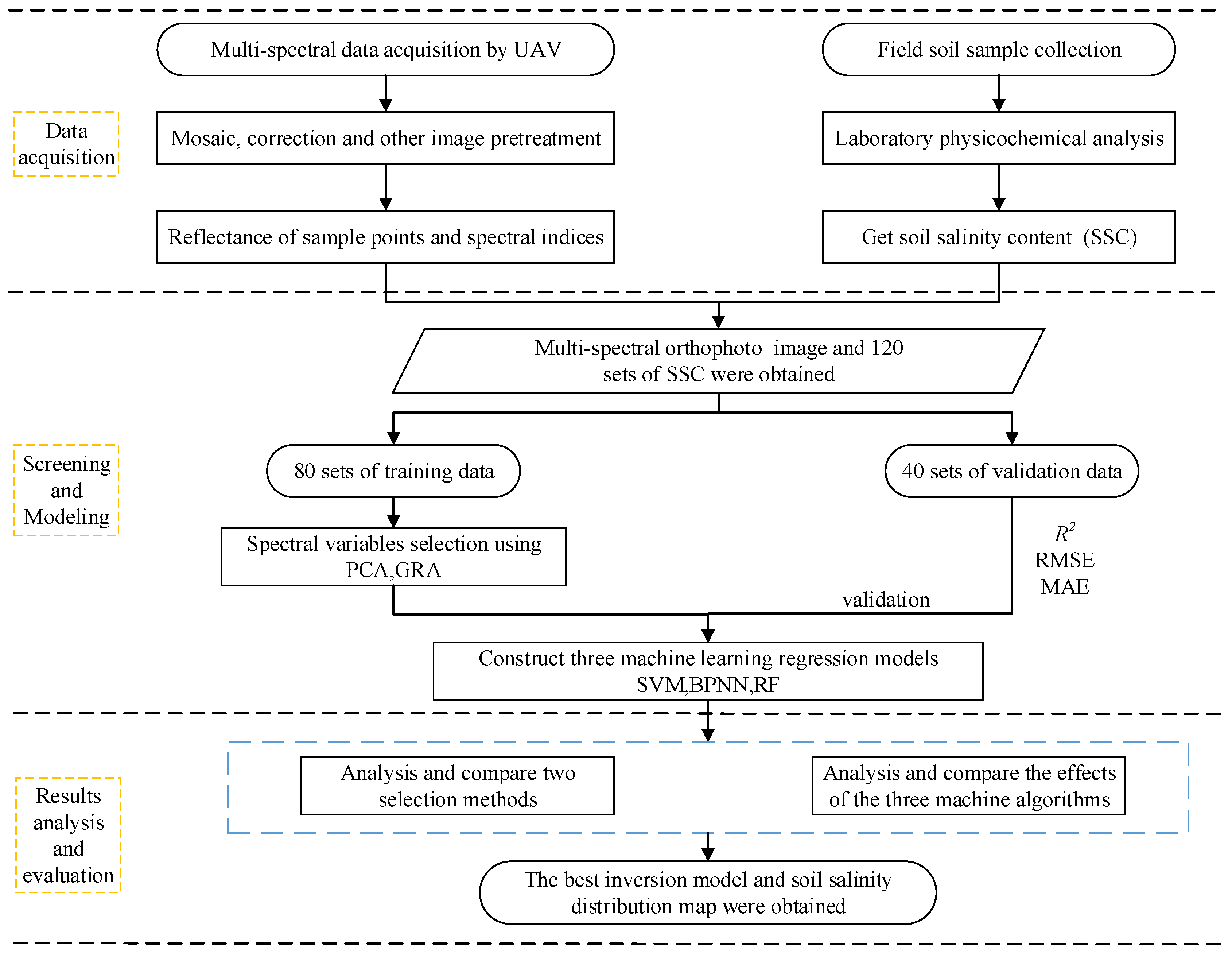
2. Materials and Methods

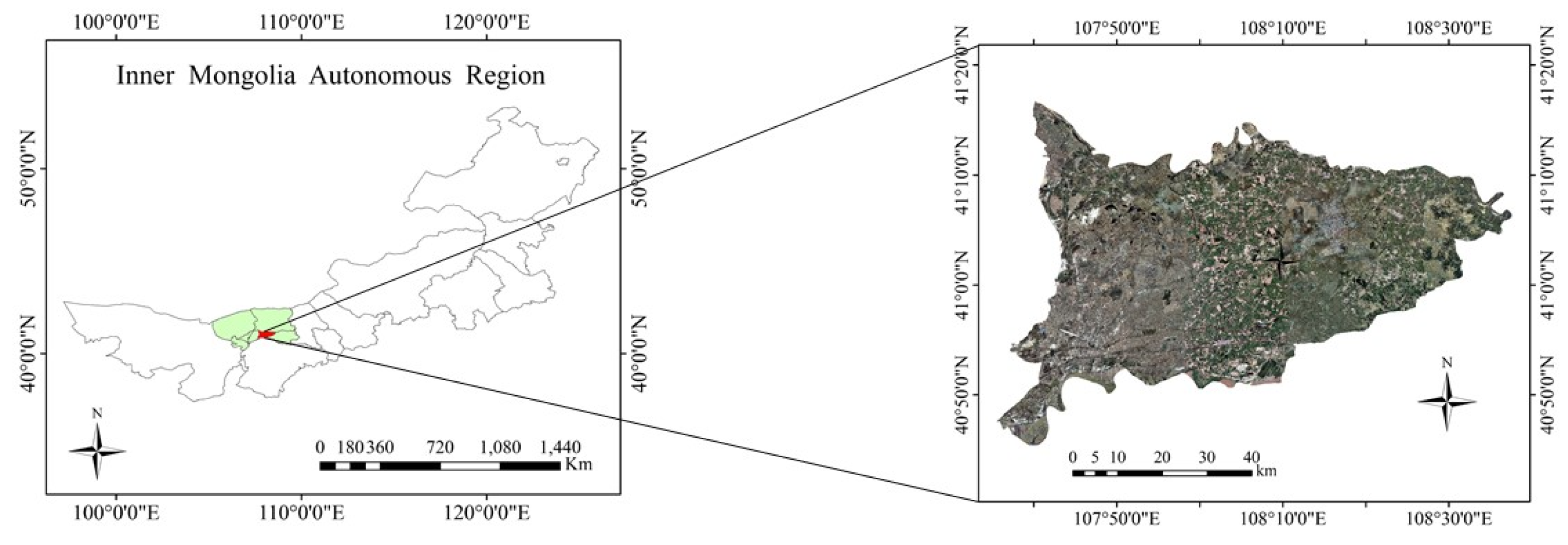
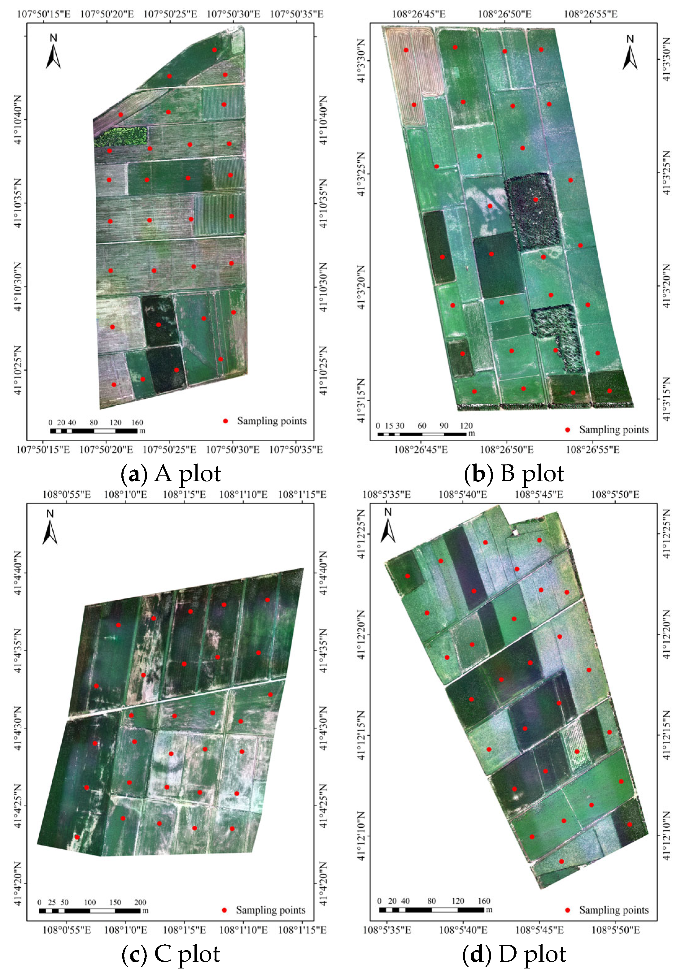
2.1. Study Area and Data Acquisition

2.1.1. Study Area

The research area is located within the Hetao Irrigation District of Wuyuan County, Bayannur City, Inner Mongolia Autonomous Region (Figure 1). The geographical coordinates are 107°35′70″–108°37′50″E and 40°46′30″–41°16′45″N, with an average altitude of 1102 m. The region belongs to the temperate continental monsoon climate, which is characterized by sufficient sunshine, large temperature differences between day and night, and low and concentrated rainfall. The annual average temperature is 7.0 °C, the average wind speed is 2.6 m/s, the annual sunshine hours are 3193 h, the annual average precipitation is 169 mm, and the annual evaporation is 2067 mm. Due to the unreasonable irrigation practices for many years, the region has had a high underground water level. When combined with the climate condition and geological features, the influence of such factors causes more than half of the arable land to face different levels of soil salinization and food production. Such land degradation is gradually increasing, seriously compromising the sustainable development of local agriculture.

2.1.2. Soil Moisture and Salt Data Collection

The experiment was conducted from 16 to 21 July 2021 in Wuyuan County. After a field investigation into the domestic planting structure and crop growth status, four representative regions were selected as sampling areas, as shown in Figure 2. Corn, sunflower, and zucchini were mainly planted in the sample area during this period. The sample collection time of ground-measured soil data is concentrated from 11:00 to 13:00 LT (centered at noon) every day, which is synchronized with the flight time of the UAV. Thirty sampling points were evenly arranged in each test site, and soil samples with two depths of 0–20 cm and 20–40 cm were collected at each sampling point. Meanwhile, the geographic coordinates of each sampling point were recorded. First, the soil samples collected in the field were divided into two parts after removing impurities. One part was put into the aluminum box, and the number and quality of the aluminum box were recorded. After being brought back to the laboratory, the aluminum box was put into the oven with the lid removed. After drying for eight hours at 105 °C, the soil moisture content (SMC) of the samples was measured and recorded using the drying method. Then, the other part of the soil sample was processed through natural air drying, grinding, and screening, and the soil solution (the ratio of soil to distilled water is 1:5) was configured. After stirring, standing, precipitation, and filtration, the conductivity value EC1:5 of the supernatant in the soil solution was measured with a conductivity instrument (DDS-307A, INESA, Shanghai, China). Each sample was measured three times, and the average value was taken as the conductivity value at the sample point after recording the data. Finally, the soil salt content (SSC) is calculated using an empirical formula, and the unit is g/100 g, expressed as a percentage [32].

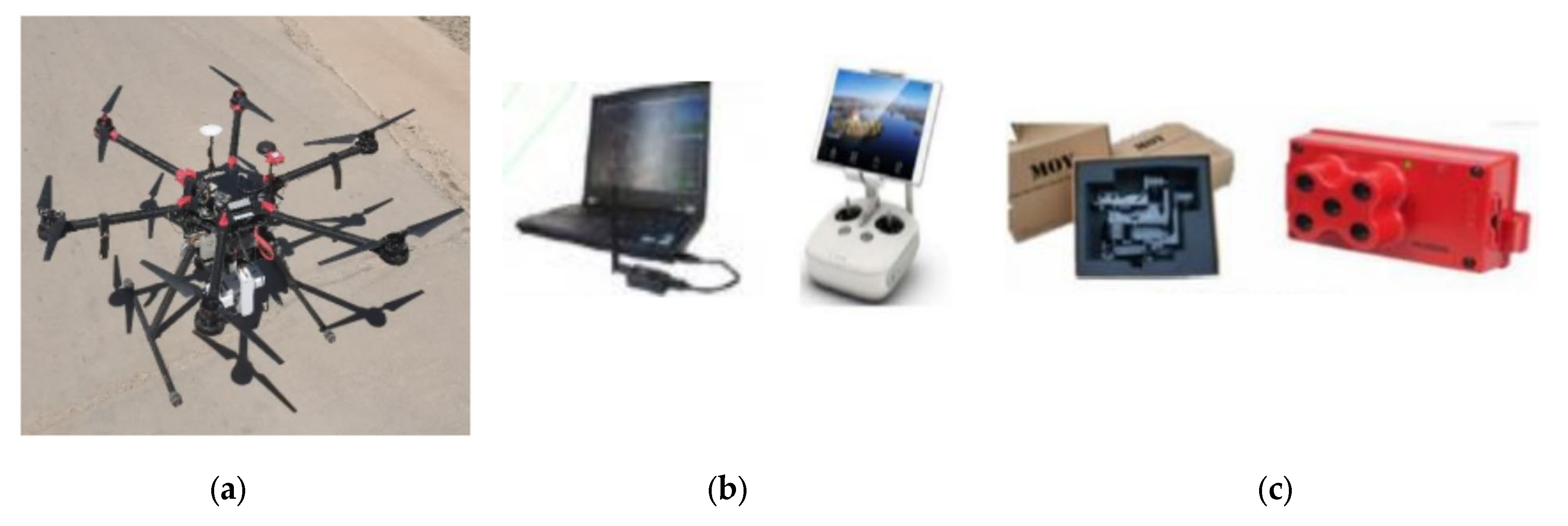
2.1.3. UAV Remote Sensing Image Data Acquisition and Processing

This part of data collection is based on the self-developed UAV multi-spectral remote sensing image acquisition system (Figure 3), and its parameter setting is referenced in the literature [33]; the platform stands on a DJI S900, with a takeoff weight of 6 kg and a maximum flight time of 30 min. The system is equipped with a Rededge-M Multi-spectral camera (Micasense, Wichita, KS, USA), which has five spectral acquisition channels: Blue-475 nm, Green-560 nm, Red-668 nm, Rededge-717 nm, Nir-840 nm. Before the UAV takes off, the ground fixed reflectance correction board (Group VIII) should be photographed so that the correct reflectance correction coefficient can be imported into the image mosaic. Then, the multi-spectral image of the sampling area can be obtained.

The UAV multi-spectral-image-acquisition time was synchronized with the ground soil sampling time, and the weather was clear, cloudless, and sunny during the flight. The UAV flew at an altitude of 100 m, and the multi-spectral camera lens was oriented vertically down, with a heading and lateral overlap of 85%. In order to obtain accurate orthophoto images, four ground control points were set up on each block before takeoff, and the three-dimensional coordinates of each control point were determined using a portable RTK measuring instrument (i50, CHCNAV, Shanghai, China). After the flight, the UAV image data were spliced using Pix4DMapper 4.5.6 software. The main splicing process was as follows. First, import the original image into ENVI 5.3 and set the output coordinate system as China 2000 for the first step of stitching. Then, import coordinate data of ground control points for geometric correction, and the generated point cloud was the radiometric correction. Finally, the orthographic image of the sample area with a ground resolution of 0.07 m was obtained. Then, the coordinate information of the orthophoto image and measured soil samples was imported into ENVI 5.3 software to determine the positions of various points in the image. Finally, the corresponding spectral reflectance of five bands was obtained.

2.2. Construction of Spectral Index

Using the spectral reflectance extracted from UAV remote sensing images, various spectral indices can be constructed through different mathematical combinations, and good results have been achieved in inverting soil salt content based on spectral indices. In this paper, some spectral indexes commonly used for soil salinization monitoring were selected; included among them were 10 Vegetation Indexes: the Simple Ratio index (SR), Difference Vegetation Index (DVI), Enhanced Vegetation Index (EVI), Atmospherically Resistant Vegetation Index (ARVI), Soil Adjusted Vegetation Index (SAVI), Canopy Response Salt Index (CRSI), Normalized Difference Vegetation Index (NDVI), Greenness Normalized Difference Vegetation Index (GNDVI), Modified Soil-Adjusted Vegetation index (MSAVI), Rededge Normalized Difference Vegetation Index (NDVI-reg). Ten salt indexes were as follows: the Salt Index (SI), Salt Index-1 (SI1), Salt Index-2 (SI2), Salt Index-3 (SI3), Salt Index1 (S1), Salt Index2 (S2), Salt Index3 (S3), Salt Index5 (S5), Salt Index6 (S6), and the Salt Index-T (SI-T). Their calculation methods are shown in

Table 1. Spectral indexes and related formula.

Vegetation Index	Formulas	References	Salt Index	Formulas	References
SR	$Nir/Red$	[34]	SI	$\sqrt{Blue\times Red}$	[35]
DVI	$Nir-Red$		SI1	$\sqrt{Red\times Green}$
EVI	$2.5\times \left(\frac{Nir-Red}{N\mathrm{ir}+6Red-7.5Blue+1}\right)$		SI2	$\sqrt{Gree{n}^2+Re{d}^2+Ni{r}^2}$
ARVI	$\frac{Nir-(2Red-Blue)}{Nir+(2Red-Blue)}$		SI3	$\sqrt{Gree{n}^2+Re{d}^2}$
SAVI	$\left(\frac{Nir-Red}{N\mathrm{ir}+Red+0.5}\right)\times \left(1+0.5\right)$		S1	$Blue/Red$
CRSI	$\sqrt{\frac{\left(Nir\times Red\right)-\left(Green\times Red\right)}{\left(Nir\times Red\right)+\left(Green\times Red\right)}}$		S2	$\frac{Blue-Red}{Blue+Red}$
NDVI	$\frac{Nir-Red}{Nir+Red}$		S3	$\frac{Green\times Red}{Blue}$
GNDVI	$\frac{Green-Red}{Green+Red}$	[36]	S5	$\frac{Blue\times Red}{Green}$
MSAVI	$\frac{(2Nir-1)-\sqrt{{(2Nir+1)}^2-8(Nir-Red)}}{2}$	[37]	S6	$\frac{N\mathrm{ir}\times Red}{Green}$
NDVI-reg	$\frac{Nir-Rededge}{Nir+Rededge}$	[34]	SI-T	$(Red-Nir)\times 100$

Note: Blue, Green, Red, Rededge, and Nir are the spectral reflectances at 475 nm, 560 nm, 668 nm, 717 nm, and 840 nm wavelengths.

.

2.3. Variable Filtering Methods

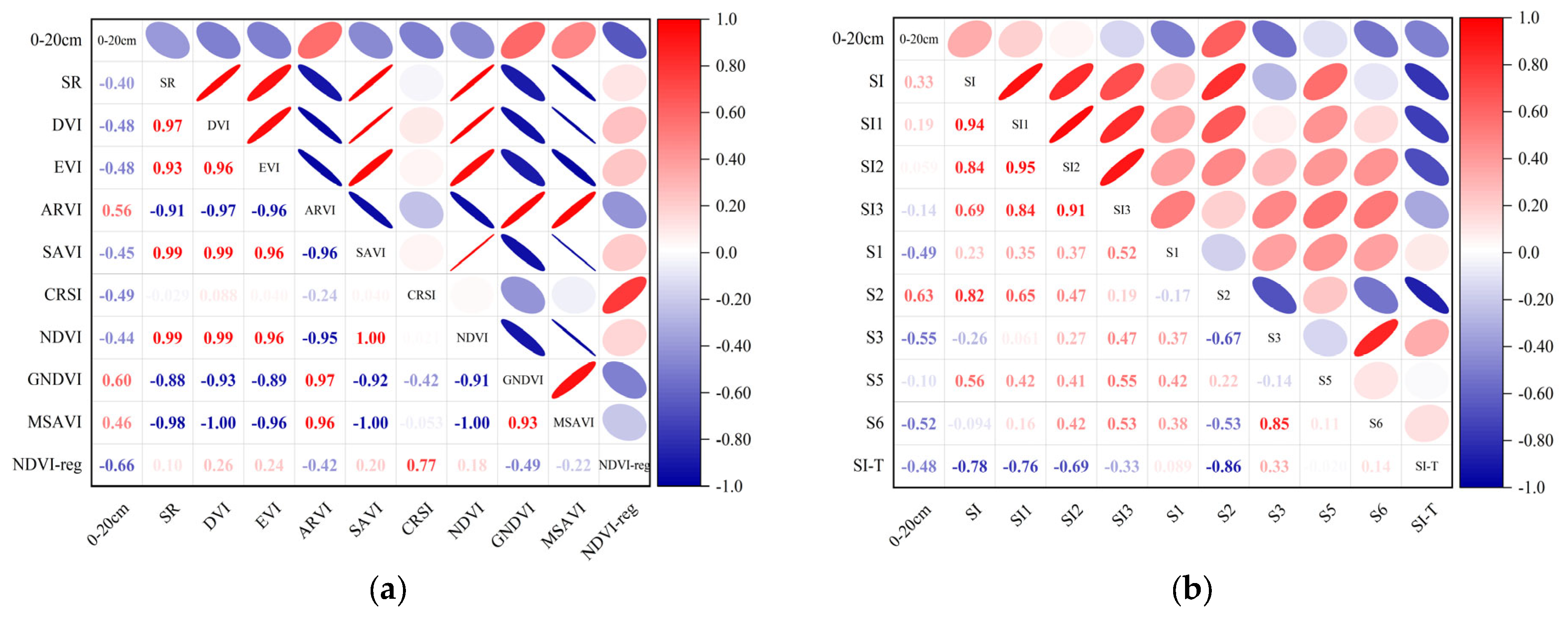
2.3.1. Pearson Correlation Analysis Method (PCA)

In statistics, the Pearson correlation coefficient (PCC) is used to measure the correlation between two variables, and its value is between −1 and 1. The greater the absolute value of the correlation coefficient, the greater the correlation between them [38]. This method is widely used in variable screening and can effectively reduce redundant variables. Assuming that n different samples ${\left\{\left(X_i,Y_i\right)\right\}}_{i=1^n}$ are available, the Pearson correlation coefficient value (r) can be calculated using Equation (1):

$$r=\frac{{\displaystyle {\sum }_{i=1}^n(X_i-\overline{X})(Y_i-\overline{Y})}}{\sqrt{{\displaystyle {\sum }_{i=1}^n{(X_i-\overline{X})}^2}}\sqrt{{\displaystyle {\sum }_{i=1}^n{(Y_i-\overline{Y})}^2}}}$$

(1)

where $X_i$ and $Y_i$ represent the measured values of two input attributes and $\overline{X}$ $\overline{Y}$ represent the mean values of them. Our PCA used IBM SPSS Statistics 26 to represent the mean values.

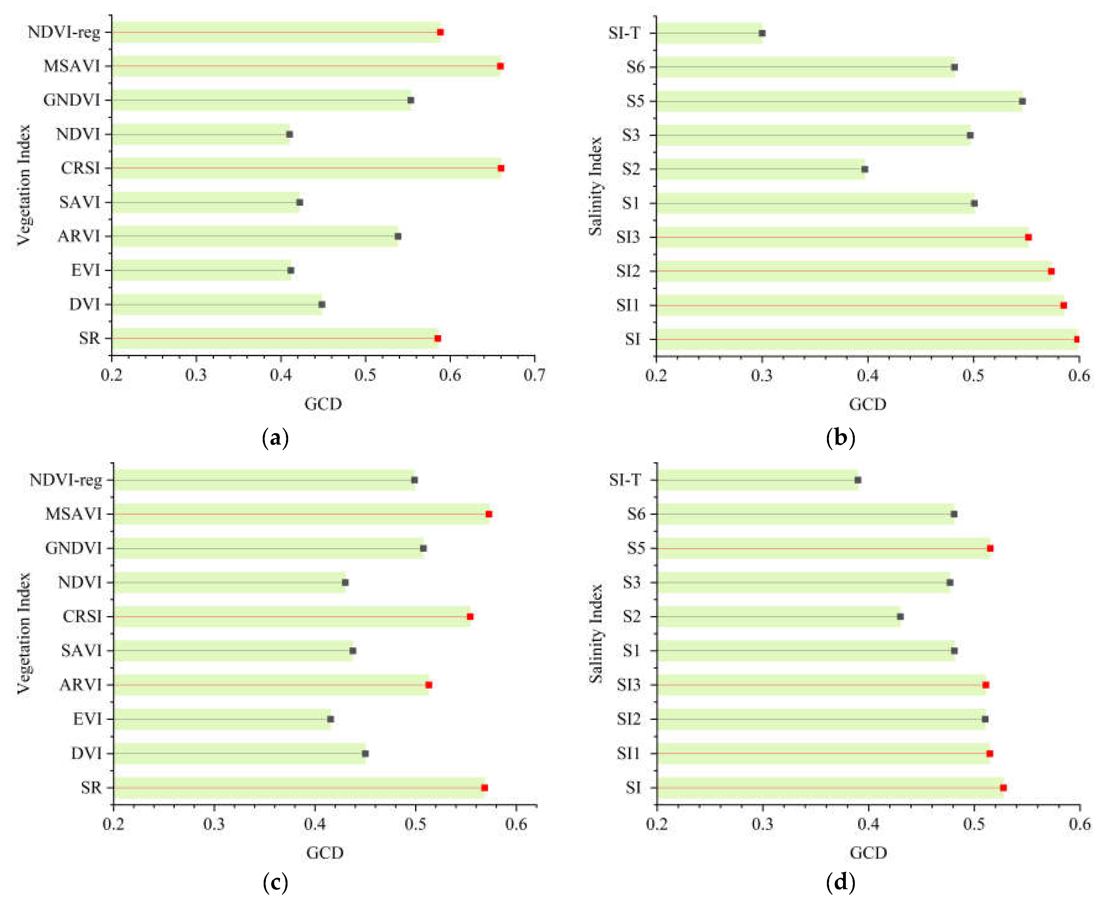
2.3.2. Grey Relational Analysis Method (GRA)

GRA is a multi-factor statistical analysis method. Its basic principle is as follows. If the changing trend of two factors is consistent, that is, if the degree of synchronous change is high, the correlation degree between the two factors will be high. Otherwise, the correlation degree is low [39]. Its performance in clarifying complex interrelationships between the multifactor and variables has been widely used. Assuming that $X_0=\left\{x_0(t),t=1,2,\cdots ,n\right\}$ and $X_i=\left\{x_i(t),t=1,2,\cdots ,n\right\}$ are defined as the reference sequence and comparison sequence, respectively, the grey correlation degree GCD can be calculated using Equation (2):

$$\begin{array}{l}GCD=\frac{1}{n}{\displaystyle \sum _{t=1}^n\gamma (x_0(t),x_i(t))}\gamma (x_0(t),x_i(t))\\ =\frac{\underset{i}{min} \underset{t}{min}\left|x_0(t)-x_i(t)\right|+\xi \underset{i}{max} \underset{t}{max}\left|x_0(t)-x_i(t)\right|}{\left|x_0(t)-x_i(t)\right|+\xi \underset{i}{max} \underset{t}{max}\left|x_0(t)-x_i(t)\right|}\end{array}$$

(2)

where ξ is the distinguishing coefficient with a range of [0, 1], in this study, setting ξ = 0.5. GRA is completed by the data processing software DPS 7.05.

2.4. Model Construction and Accuracy Evaluation

2.4.1. Machine Learning Models

In this study, variables after feature screening were taken as independent variables, and the soil salt contents (SSCs) at different depths were taken as dependent variables. Three machine learning regression models, namely a Support Vector Machine (SVM), Random Forests (RF), and a Back Propagation Neural Network (BPNN) were constructed by the software R 4.1.3. The estimation effects of three models on the soil salt content (SSC) were compared and analyzed. The technology roadmap is shown in Figure 4.

SVM operates based on statistical learning theory, specifically on the theory of the structural risk minimization principle, from a linear separable extended to a linear inseparable new machine learning method, and can effectively classify and perform regression. In recent years, with its characteristics of simple structure and strong adaptability, extracting the soil water and salt content in inversion has been widely applied [40,41]. The SVM was implemented using the “e1071” package in R 4.1.3. The optimal parameters, cost = 4 and gamma = 0.1, were determined based on a 10-fold cross-validation and grid search method, and the other parameters were the default values.

BPNN is a multi-layer feedforward error reversal neural network, of which output results are propagated forward, and errors are propagated back. The input layer, the hidden layer, and the output layer constitute the topology of the model. With its strong fitting ability, it has become a common prediction model [42]. BPNN was implemented using the “nnet” package in R 4.1.3. The optimal parameters, decay = 0.001 and size = 4, were determined based on a 10-fold cross-validation and grid search method, and the other parameters were the default values.

RF is a classification regression model, which contains multiple decision trees, and the output category is determined by the mode of the category output by individual trees. It is an integrated learning algorithm based on a bagging and a decision tree algorithm. It does not require distribution assumptions about the relationship of response covariables. The process allows for statistically reliable estimates of model generalization capability without the risk of overfitting [43]. RF was performed using the “Random Forest” package in R 4.1.3, and the optimal parameters, ntree = 1000 and mtry = 2, were determined based on a 10-fold cross-validation and grid search method, and the other parameters were the default values.

2.4.2. Accuracy Evaluation

To ensure that the training set and validation set can represent the statistical data characteristics of samples, 120 ground-measured data were divided by the function “Create Data Partition” in the R 4.1.3 “caret” package. Two-thirds of the samples (n = 80) were selected as the training set, and one-third of the samples (n = 40) comprised the validation set. The model accuracy was verified based on the fitting effect of the actual measured values of validation-set samples and the estimated values of the model. The coefficient of determination (R²), Root-Mean-Square-Error (RMSE), and Mean Absolute Error (MAE) were used to evaluate the validation accuracy of the model. R² ranges from 0 to 1. The closer R² is to 1 and the smaller RMSE and MAE are, the better the prediction effect of the model is. The relevant equations are given as follows:

$$R^2=\frac{{\displaystyle \sum _{i=1}^n{({\widehat{y}}_i-\overline{y})}^2}}{{\displaystyle \sum _{i=1}^n{(y_i-\overline{y})}^2}}$$

(3)

$$RMSE=\sqrt{\frac{1}{n}{\displaystyle \sum _{i=1}^n{({\widehat{y}}_i-y_i)}^2}}$$

(4)

$$MAE=\frac{1}{n}{\displaystyle \sum _{i=1}^n\left|y_i-{\widehat{y}}_i\right|}$$

(5)

where $y_i$ is the measured value of the soil salt content, ${\widehat{y}}_i$ is the predicted value of the soil salt content, $\overline{y}$ is the average value of the soil salt content, and n is the number of samples.

3. Results

3.1. Statistical Analysis of Soil Salt Data

Statistical analysis was conducted on the salt content of soil samples in the study area. It can be seen from the results in

Table 2. Statistical analysis of soil salt content measured data.

Soil Depths (cm)	Data Sets	Total	Min (%)	Max (%)	Average (%)	Median (%)	Standard Deviation (%)
0–20	Total sample	120	0.070	0.503	0.151	0.107	0.097
	Training set	80	0.070	0.503	0.144	0.107	0.090
	Validation set	40	0.074	0.488	0.158	0.108	0.109
20–40	Total sample	120	0.073	0.556	0.162	0.128	0.097
	Training set	80	0.076	0.556	0.164	0.128	0.101
	Validation set	40	0.073	0.521	0.160	0.133	0.090

that the statistical indexes of the training set and verification set at various depths are close to the overall data, indicating that the training set and validation set can represent the whole dataset, and the sampling point can accurately reflect the salinization degree of the sample area. According to the soil salinization degree classification standard, the salinization degree in the sample area was evaluated as a whole. Most of the study area was slightly salinized, while some areas were severely salinized, which was basically consistent with the growth status of crops in the study area.

3.2. Screening of Spectral Index

PCA was used to analyze the correlation between the salt content of 0–20 cm and 20–40 cm soil depths and the spectral index mentioned in Section 2.2, thereby enabling the calculation of the Pearson correlation coefficient (PCC). The larger the absolute value of the PCC was, the stronger the correlation, as shown in Figure 5. At the same time, GRA was applied to analyze the correlation between the salt content in 0–20 cm and 20–40 cm soil depths and the spectral index, allowing the Grey correlation degree (GCD) to be calculated. The larger the GCD was, the stronger the correlation degree, as shown in Figure 6.

Among the correlation analyses between the vegetation index of 0–20 cm and soil salt content, NDVI-reg had the highest correlation, and the absolute value of its correlation coefficient |r| was 0.66, followed by GNDVI, ARVI, and CRSI (Figure 5a). Among the correlation analyses between the salt index and soil salt content of 0–20 cm, S2 has the highest correlation, and the absolute value of its |r| was 0.63, followed by S3, S1, and SI-T (Figure 5b). In the correlation analysis between the vegetation index of 20–40 cm and soil salt content, NDVI-reg also had the highest correlation, and the absolute value of its |r| was 0.51, followed by GNDVI, ARVI, and DVI (Figure 5c). Among the correlation analyses between the salt index and soil salt content of 20–40 cm, S1 had the highest correlation, and the absolute value of its |r| was 0.49, followed by S2, S3, and SI-T (Figure 5d).

Among them, in the gray correlation analysis of the 0–20 cm vegetation index and soil salt content, CRSI has the highest correlation, and its correlation GCD was 0.660, followed by MSAVI, NDVI-reg, and SR (Figure 6a). In the gray correlation analysis of the 0–20 cm salt index and soil salt content, SI had the highest correlation degree, and its correlation degree GCD was 0.598, followed by SI1, SI2, and SI3 (Figure 6b). In the gray correlation analysis between the vegetation index and soil salt content of 20–40 cm, MSAVI had the highest correlation degree, and its correlation degree was 0.573, SR, CRSI, and ARVI (Figure 6c). In the gray correlation analysis between the salt index and soil salt content of 20–40 cm, SI had the highest correlation degree, and its correlation degree GCD was 0.528, followed by S5, SI1, and SI3 (Figure 6d).

3.3. Soil Salt Content Inversion Model Based on Machine Learning Methods

Through Pearson correlation analysis (PCA) and Grey relational analysis (GRA) of the spectral index and the SSC in Section 3.2, the model’s input variables were determined, respectively, for the two variable screening methods. In this way, the three machine learning regression models of SVM, BPNN, and RF were established. For PCA, the top four absolute values of PCC from large to small were selected as the input variables of two groups, namely the vegetation index group and the salt index group. At the same time, to simplify spectral information and explore the influence of soil moisture information and other factors on SSC monitoring, the top two absolute values of PCC for the vegetation index and salt index and SMC were selected as a combination variable group where the model input variables were divided into three groups. Similarly, for the grey correlation analysis, three model input variable groups were set according to the above method.

Table 3. Grouping of model input variables.

Methods	Soil Depth (cm)	Vegetation Index Groups	Salt Index Groups	Combination Variable Groups
PCA	0–20	NDVI-reg, GNDVI, ARVI, CRSI	S2, S3, S1, SI-T	NDVI-reg, GNDVI, S2, S3, SMC
	20–40	NDVI-reg, GNDVI, ARVI, DVI	S1, S2, S3, SI-T	NDVI-reg, GNDVI, S1, S2, SMC
GRA	0–20	CRSI, MSAVI, NDVI-reg, SR	SI, SI1, SI2, SI3	CRSI, MSAVI, SI, SI1, SMC
	20–40	MSAVI, SR, CRSI, ARVI	SI, S5, SI1, SI3	MSAVI, SR, SI, S5, SMC

lists the specific grouping information.

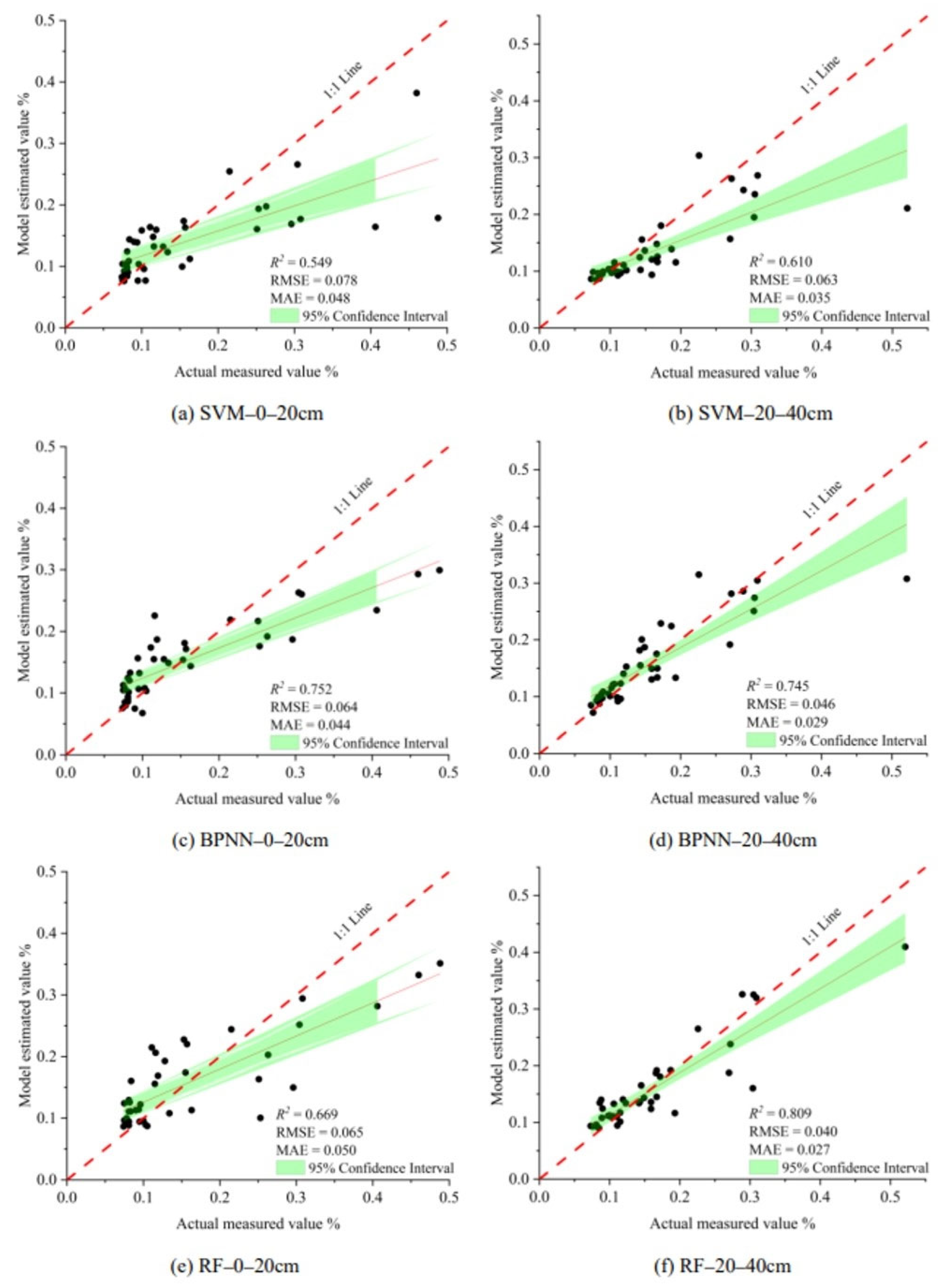
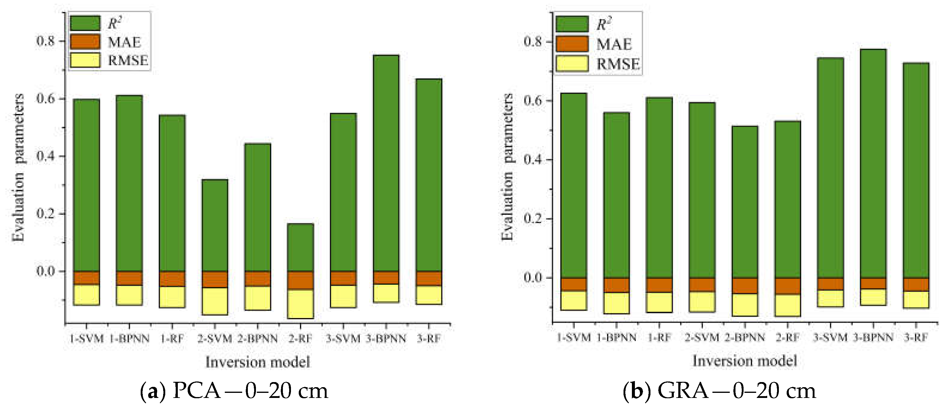
3.3.1. Inversion Model of SSC Using PCA Variable Selection Method

Based on the vegetation index group, salt index group, and combination variable group, SVM, BPNN, and RF machine learning algorithms were used to build soil salt estimation models at different depths. The model results are shown in

Table 4. Inversion results of soil salt based on the Pearson correlation analysis method.

Input Variable Groups	Model Algorithm	Soil Depths (cm)
		0–20			20–40
		R2	RMSE	MAE	R2	RMSE	MAE
Vegetation index group	SVM	0.598	0.071	0.046	0.392	0.077	0.051
	BPNN	0.612	0.069	0.048	0.262	0.078	0.058
	RF	0.543	0.074	0.052	0.290	0.077	0.054
Salt index group	SVM	0.319	0.094	0.057	0.279	0.079	0.052
	BPNN	0.444	0.084	0.051	0.326	0.074	0.054
	RF	0.165	0.101	0.063	0.226	0.080	0.056
Combination variable group	SVM	0.549	0.078	0.048	0.610	0.063	0.035
	BPNN	0.752	0.064	0.044	0.745	0.046	0.029
	RF	0.669	0.065	0.050	0.809	0.040	0.027

. From the perspective of the model input variable groups, the combination variable group was the best at both soil depths, followed by the vegetation index group and the salt index group. The linear fitting diagram of the measured soil salt value and the model estimated value of the optimal input variable group (combination variable group) are shown in Figure 7. From the perspective of the machine learning algorithm, at 0–20 cm, the BPNN model in the combination variable group had the best performance; its R², RMSE, and MAE values were 0.752, 0.064, and 0.044 (Figure 7c); at 20–40 cm, the RF model in the combination variable group had the best performance; its R², RMSE, and MAE values were 0.809, 0.040, and 0.027 (Figure 7f). From the modeling effect of different depths, the average value of the whole R² at 0–20 cm was 0.517; the modeling effect at 0–20 cm was better than that at 20–40 cm.

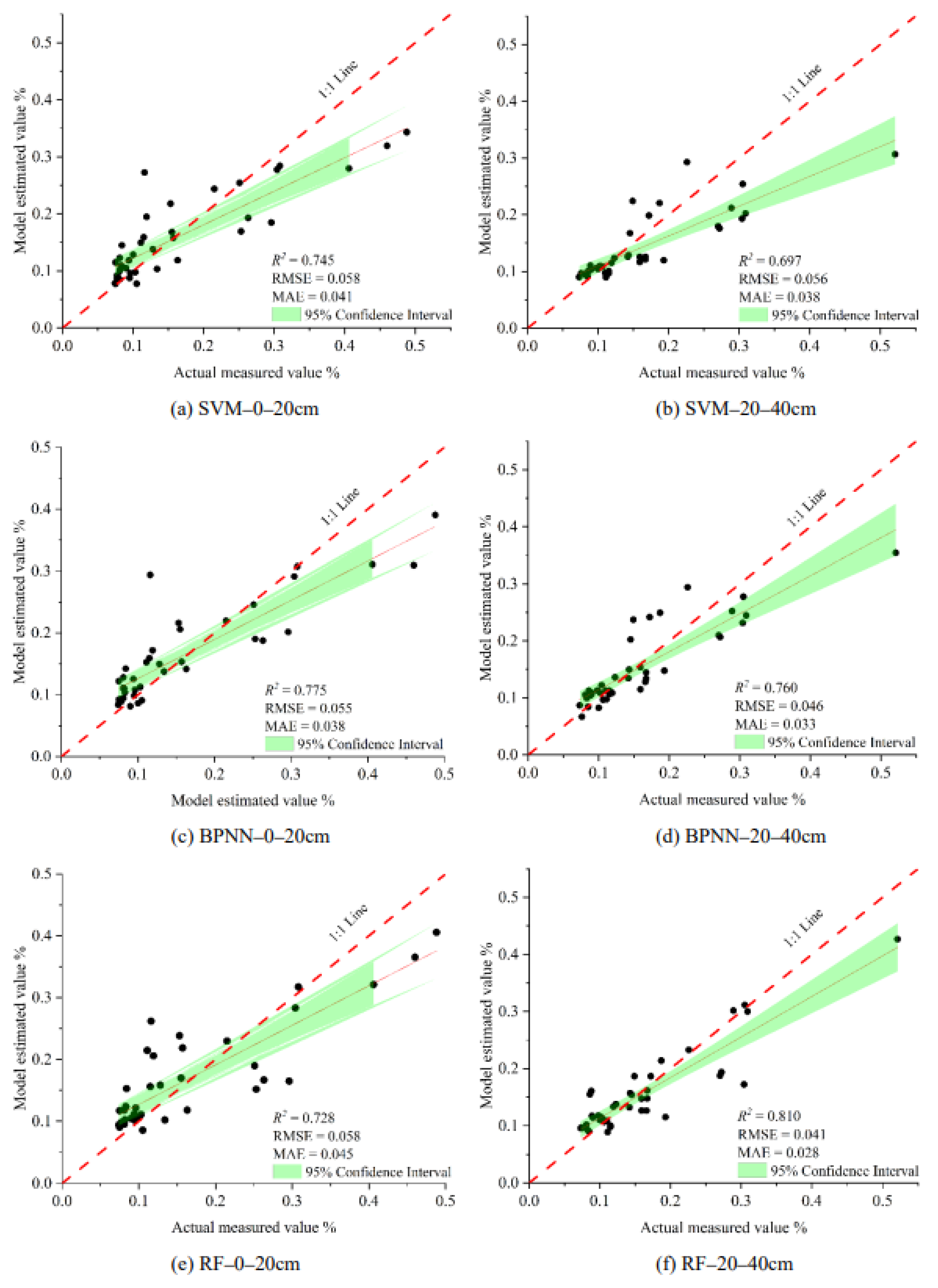
3.3.2. Inversion Model of SSC Using GRA Variable Selection Method

Based on the vegetation index group, salt index group, and combination variable group, SVM, BPNN, and RF machine learning algorithms were used to build soil salt estimation models at different depths. The model results are shown in

Table 5. Estimation results of soil salt based on Grey relation analysis method.

Input Variable Groups	Model Algorithm	Soil Depths (cm)
		0–20			20–40
		R2	RMSE	MAE	R2	RMSE	MAE
Vegetation index groups	SVM	0.626	0.066	0.044	0.468	0.068	0.046
	BPNN	0.560	0.072	0.050	0.444	0.070	0.053
	RF	0.611	0.069	0.049	0.214	0.083	0.060
Salt index groups	SVM	0.594	0.069	0.047	0.539	0.066	0.048
	BPNN	0.514	0.076	0.054	0.473	0.070	0.052
	RF	0.531	0.075	0.056	0.195	0.082	0.063
Combination variable groups	SVM	0.745	0.058	0.041	0.697	0.056	0.038
	BPNN	0.775	0.055	0.038	0.760	0.046	0.033
	RF	0.728	0.058	0.045	0.810	0.041	0.028

. The overall prediction results of the model were similar to those in Table 4, and the estimation accuracy was improved, but there were also some differences. The combination variable group was still the best at the two soil depths. Notably, however, the overall estimation accuracy of the salt index group was higher than that of the vegetation index group at depths of 20–40 cm, which was different from the results in Section 3.3.1. The average value of the overall R² at 0–20 cm was 0.632, higher than 0.517 in Section 3.3.1, and the average value of the overall R² at 20–40 cm was 0.511, which was also higher than 0.438 in Section 3.3.1. At 0–20 cm, the BPNN model in the combination variable group had the best performance; its R², RMSE, and MAE values were 0.775, 0.055, and 0.038 (Figure 8c); at 20–40 cm, the RF model in the combination variable group had the best performance; its R², RMSE, and MAE values were 0.810, 0.041, and 0.028 (Figure 8f). Figure 8 shows the linear fitting diagram of the measured soil salt value and the model-estimated value of the optimal input variable group (combination variable group).

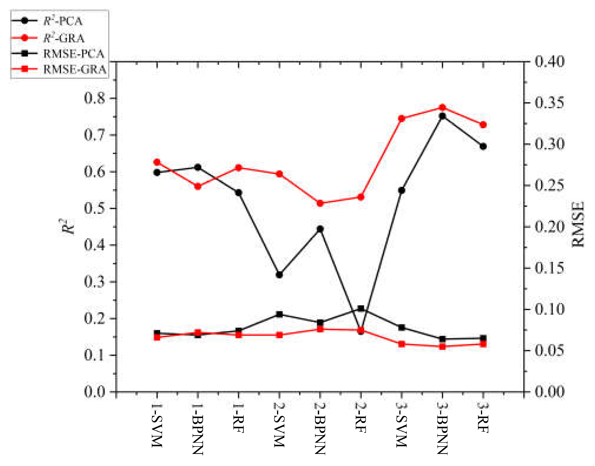
3.4. Comprehensive Evaluation and Analysis of the Models

Table 4 and Table 5 show the comparative analysis of the GRA method after screening. The estimation accuracy of modeling was overall superior to the PCA method used to build the model. After screening three groups of model input variables, the combination variable group performed best, and the optimal group at different depths of the estimation model were all from the combination variables group. In this paper, evaluation parameters of the validation set R², RMSE, and MAE were used to draw the accumulation histogram of each model (Figure 9), to further intuitively analyze the differences between models. The vegetation index group, salt index group, and combination variable group were numbered 1, 2, and 3, accordingly. As shown in Figure 9, the stability of the soil salt estimation models with different depths established by using two variable screening methods and three machine learning algorithms was good in most cases, and the RMSE and MAE values were within a reasonable range. The Grey relational analysis method can effectively remove redundant spectral information and improve the estimation accuracy of the model. Although there are some models with high estimation accuracy at a 20–40 cm soil depth, when the stability and estimation accuracy of the model were considered comprehensively, the comparative analysis showed that the stability and prediction accuracy of the inversion model at 0–20 cm were better than those at 20–40 cm, and the best estimation model was GRA-3-BPNN (Figure 9b). Finally, based on the best estimation model, a soil salt distribution map of the 0–20 cm soil depth in the study area was drawn. As seen in Figure 10, soil salinization in the four sample areas in the study area was mostly characterized by slight salinization, with severe salinization in some parts. The severe salinization in the northwest of B plot affected the normal growth of crops even after sowing, resulting in bare soil in the area. There was an area of moderate salinization concentrated in the southeastern part of C plot, and the salt-tolerant crop sunflower is mainly planted in this area, which is consistent with the actual survey situation; at the same time, there was salinization in part of the plots A and D. Therefore, the salt distribution map can be used for soil improvement, salt drainage control, and salinization prevention in the corresponding plots in the study area, and salt-tolerant crops, such as sunflower, can be planted.

4. Discussion

4.1. Comparison of Variable Filtering Methods

Using optical remote sensing to determine the crop growth status and indirectly inverting soil salt content (SSC) is still a commonly used monitoring method. It mainly establishes a certain relationship among the reflectance, spectral index, and SSC and then estimates soil salt in the crop root zone [44,45]. However, the optical remote sensing information is complex, and if the redundant spectral information is not screened, the stability and accuracy of the monitoring model will be affected [46]. In this paper, the two variable screening methods (PCA and GRA) were used to screen the spectral variables effectively, and some indices with a weak correlation or a poor correlation degree were removed to improve the efficiency of the monitoring model. The experimental results show that the salt monitoring model, established according to the screening of two variables, has good overall performance, and the model built based on GRA has a higher overall estimation accuracy. As shown in Figure 11, taking soil depth of 0–20 cm as an example, GRA is superior to PCA in both estimation accuracy and model stability according to the distribution of the model evaluation indexes R² and RMSE in the figure. The nature of the PCA is a linear relationship, and the nonlinear relationship between prediction variables and target variables may be ignored in experiments since GRA almost does not exist in these problems [43]. In the literature [14], the GRA method was used to screen sensitive variables and estimate the SSC information of sunflowers for two growth stages in the field.

4.2. Comparative Analysis of Related Studies

Soil salinization is a common problem facing the world, and the efficient and accurate acquisition of soil salt information is crucial. Crops mainly obtain nutrients from the soil through their roots. The increase in soil salt in the root zone of plants greatly affects the absorption of nutrients by crops. Under this stress, plant growth undergoes changes, and higher soil salt in the root zone of crops can lead to increased salt stress and the deterioration of growth conditions [47,48]. There have been some previous studies on this; based on soil electrical conductivity (SEC) and VIS-NIR spectroscopy data, Cao et al. [49] used BPNN, SVM, and ELM algorithms to estimate SEC and introduced partial least squares regression (PLSR) for comparison. The final results show that the machine learning algorithm can improve the estimation accuracy of the model compared with PLSR. Similarly, the three machine learning regression models used in this study also show good results; the optimal estimation results of the SVM, BPNN, and RF models were between 0.745 and 0.810. Khosravi et al. [50] estimated the heavy metal content in soil using a machine learning algorithm, and the results showed that ELM models had a better effect than PLSR models; Nawar et al. [51] compared the PLSR, SVM, and MARS methods for predicting the soil clay content and organic matter, and the results showed that in most cases, MARS and SVR models performed better than PLSR models. Therefore, the author believes that machine learning algorithms will have broad application prospects regarding the quantitative estimation of soil properties.

In this study, it can be found that different model input variables also impact prediction accuracy. Among the three input variable groups in this paper, the combination variable group containing SMC data performs best. Zhang et al. [52] show that both water and salt in soil can affect the spectrum in different ways, and the water–salt interaction model can improve the simulation effect of the soil surface spectrum. Therefore, it can be seen that soil water has an important influence on the estimation of SSC. The estimation effect at 0–20 cm was the best among the two soil depths, which is basically similar to the results in the literature [37]. The soil at a depth of 0–20 cm contains the main root layer of crops, and the influence of soil salt on crop growth is closely related to the root of the plant.

4.3. Summary and Prospects

Optical remote sensing of the crop canopy is used to monitor soil salt. Yet, altered spectral characteristics of the crop canopy are not always attributed to soil salt, noting that changes in soil moisture, nutrients, and other factors will also affect the spectral characteristics of the canopy [53]. Using reflectance values and the DEM of the Landsat 7 satellite in the winter and summer of 2013, Yahiaoui et al. [54] analyzed the relationship between soil salt and topographic parameters and explained the role of topographic parameters in monitoring and evaluating the spatial distribution of soil salt in the in the study area. In addition, using optical remote sensing to monitor SSC may lead to problems, such as a lack of information and unclear characteristics [55]. Ivushkin et al. [56] monitored soil salt information under crop coverage based on a multi-source remote sensing cooperative and analyzed the distribution characteristics of saline soil and its impact on vegetation growth. Therefore, in future studies, attention should be paid to the influence of soil moisture, nutrients, texture, different coverage, various crop types, and other influential factors on the monitoring effects.

It follows that future research work on soil salinization monitoring should focus on the following aspects. (1) After considering the influence of various factors on the monitoring effects, optimize the pretreatment scheme of spectral information, and improve the generalization ability of the model. (2) Combine UAV remote sensing with ground hyperspectral and satellite remote sensing, and strive to form a multi-directional integrated collaborative monitoring system.

5. Conclusions

In this study, UAV multi-spectral remote sensing technology and a machine learning algorithm were used to invert the farmland soil salt content at different depths under crop coverage, and the following conclusions could be drawn from the results.

The information contained in different spectral characteristic variables of the crop canopy in soil salt content estimations using UAV remote sensing is repeated to a certain extent. Both variable screening methods can remove irrelevant redundant spectral information to improve the model’s efficiency. Compared with the PCA method, the GRA method is more suitable for screening spectral variables, which is beneficial to improve the stability and estimation accuracy of the model.

Through a salt estimation model constructed using two variable screening methods and three machine learning algorithms, it is evident that the prediction effect of the 0–20 cm depth surface soil is better than that of the 20–40 cm depth when considering the stability and estimation accuracy of the model. The R², RMSE, and MAE of the best estimation model are 0.775, 0.055, and 0.038, respectively.

This paper chose three types of machine learning models and, to a certain extent, achieved a good prediction effect. Based on the best estimation model of salt distribution, it is evident that the results satisfactorily reflect the degree of soil salinization in the study area, indicating that this article chose an applicable method for the study of UAV remote sensing estimations of the soil salt content.

References

1. Asfaw, E.; Suryabhagavan, K.V.; Argaw, M. Soil salinity modeling and mapping using remote sensing and GIS: The case of Wonji sugar cane irrigation farm, Ethiopia. J. Saudi Soc. Remote 2016, 17, 250–258. [Google Scholar] [CrossRef]
2. Wang, F.; Shi, Z.; Biswas, A.; Yang, S.; Ding, J. Multi-algorithm comparison for predicting soil salinity. Geoderma 2020, 365, 114–211. [Google Scholar] [CrossRef]
3. Han, L.; Liu, D.; Cheng, G.; Zhang, G.; Wang, L. Spatial distribution and genesis of salt on the saline playa at Qehan Lake, Inner Mongolia, China. CATENA 2019, 177, 22–30. [Google Scholar] [CrossRef]
4. Carla, C.; Paula, P.; Maximiliano, A. Spatial and temporal patterns of soil salinization in shallow groundwater environments of the Bahía Blanca estuary: Influence of topography and land use. Land Degrad. Dev. 2022, 33, 470–483. [Google Scholar]
5. Li, Y.; Chang, C.; Wang, Z.; Zhao, G. Upscaling remote sensing inversion and dynamic monitoring of soil salinization in the Yellow River Delta, China. Ecol. Indic. 2023, 148, 110087. [Google Scholar] [CrossRef]
6. Kasim, N.; Maihemuti, B.; Sawut, R.; Abliz, A.; Dong, C.; Abdumutallip, M. Quantitative estimation of soil salinization in an arid region of the Keriya Oasis based on multidimensional modeling. Water 2020, 12, 880. [Google Scholar] [CrossRef]
7. Tan, J.; Ding, J.; Han, L.; Ge, X.; Wang, X.; Wang, J.; Wang, R.; Qin, S.; Zhang, Z.; Li, Y. Exploring planetscope satellite capabilities for soil salinity estimation and mapping in Arid Regions Oases. Remote Sens. 2023, 15, 1066. [Google Scholar] [CrossRef]
8. Zhou, X.; Zhang, F.; Zhang, H.; Zhang, X.; Yuan, J. A study of soil salinity inversion based on multispectral remote sensing index in Ebinur Lake Wetland Nature Reserve. Spectrosc. Spect. Anal. 2019, 39, 1229–1235. [Google Scholar]
9. Gholizadeh, A.; Žižala, D.; Saberioon, M.; Borůvka, L. Soil organic carbon and texture retrieving and mapping using proximal, airborne and Sentinel-2 spectral imaging. Remote Sens. Environ. 2018, 218, 89–103. [Google Scholar] [CrossRef]
10. Dehaan, R.L.; Taylor, G.R. Field-derived spectra of salinized soils and vegetation as indicators of irrigation-induced soil salinization. Remote Sens. Environ. 2002, 80, 406–417. [Google Scholar] [CrossRef]
11. Ding, J.; Yu, D. Monitoring and evaluating spatial variability of soil salinity in dry and wet seasons in the Werigan–Kuqa Oasis, China, using remote sensing and electromagnetic induction instruments. Geoderma 2014, 235–236, 316–322. [Google Scholar] [CrossRef]
12. Farifteh, J.; Van der Meer, F.; Atzberger, C.; Carranza, E.J.M. Quantitative analysis of salt-affected soil reflectance spectra: A comparison of two adaptive methods (PLSR and ANN). Remote Sens. Environ. 2007, 110, 59–78. [Google Scholar] [CrossRef]
13. Wang, L.; Zhang, B.; Shen, Q.; Yao, Y.; Zhang, Y. Estimation of soil salt and ion contents based on hyperspectral remote sensing data: A case study of Baidunzi Basin, China. Water 2021, 13, 559. [Google Scholar] [CrossRef]
14. Chen, J.; Yao, Z.; Zhang, Z.; Wei, G.; Wang, X.; Han, J. UAV remote sensing inversion of soil salinity in field of sunflower. Trans. Chin. Soc. Agric. Mach. 2020, 51, 178–191. [Google Scholar]
15. Nurmemet, I.; Ghulam, A.; Tiyip, T.; Elkadiri, R.; Ding, J.; Maimaitiyiming, M.; Abliz, A.; Sawut, M.; Zhang, F.; Abliz, A.; et al. Monitoring soil salinization in Keriya River Basin, Northwestern China using passive reflective and active microwave remote sensing data. Remote Sens. 2015, 7, 8803–8829. [Google Scholar] [CrossRef]
16. Zhang, Z.; Du, Y.; Lao, C.; Yang, N.; Zhou, Y.; Yang, Y. Inversion model of soil salt content in different depths based onadar remote sensing. Trans. Chin. Soc. Agric. Mach. 2020, 51, 243–251. [Google Scholar]
17. Chen, R.; Shang, T.; Zhang, J.; Wang, Y.; Jia, K. Effects of different spectra types on the accuracy and correction of soil salt content inversion in Yinchuan Plain. China. J. Appl. Ecol. 2022, 33, 922–930. [Google Scholar]
18. Xu, X.; Chen, Y.; Wang, M.; Wang, S.; Li, K.; Li, Y. Improving estimates of soil salt content by using two-date image spectral changes in Yinbei, China. Remote Sens. 2021, 13, 4165. [Google Scholar] [CrossRef]
19. Peng, J.; Biswas, A.; Jiang, Q.; Zhao, R.; Hu, J.; Hu, B.; Shi, Z. Estimating soil salinity from remote sensing and terrain data in southern Xinjiang Province, China. Geoderma 2019, 337, 1309–1319. [Google Scholar] [CrossRef]
20. Lao, C.; Chen, J.; Zhang, Z.; Chen, Y.; Ma, Y.; Chen, H.; Gu, X.; Ning, J.; Jin, J.; Li, X. Predicting the contents of soil salt and major water-soluble ions with fractional-order derivative spectral indices and variable selection. Comput. Electron. Agric. 2021, 182, 106031. [Google Scholar] [CrossRef]
21. Wei, G.; Li, Y.; Zhang, Z.; Chen, Y.; Chen, J.; Yao, Z.; Lao, C.; Chen, H. Estimation of soil salt content by combining UAV-borne multispectral sensor and machine learning algorithms. PeerJ 2020, 8, e9087. [Google Scholar] [CrossRef]
22. Bhardwaj, A.; Sam, L.; Akanksha; Martín-Torres, F.J.; Kumar, R. UAVs as remote sensing platform in glaciology: Present applications and future prospects. Remote Sens. Environ. 2016, 175, 196–204. [Google Scholar] [CrossRef]
23. Zaman-Allah, M.; Vergara, O.; Araus, J.L.; Tarekegne, A.; Magorokosho, C.; Zarco-Tejada, P.J.; Hornero, A.; Albà, A.; Das, B.; Craufurd, P.; et al. Unmanned aerial platform-based multi-spectral imaging for field phenotyping of maize. Plant Methods 2015, 11, 1–10. [Google Scholar] [CrossRef]
24. Peng, M.; Han, W.; Li, C.; Huang, S. Improving the spatial and temporal estimation of maize daytime net ecosystem carbon exchange variation based on unmanned aerial vehicle multispectral remote sensing. IEEE J. Sel. Top. Appl. Earth Observ. Remote Sens. 2021, 14, 10560–10570. [Google Scholar] [CrossRef]
25. Huang, S.; Han, W.; Chen, H.; Li, G.; Tang, J. Recognizing zucchinis intercropped with sunflowers in UAV visible images using an improved method based on OCRNet. Remote Sens. 2021, 13, 2706. [Google Scholar] [CrossRef]
26. Peng, X.; Han, W.; Ao, J.; Wang, Y. Assimilation of LAI derived from UAV multispectral data into the SAFY model to estimate maize yield. Remote Sens. 2021, 13, 1094. [Google Scholar] [CrossRef]
27. Zhang, L.; Zhang, H.; Han, W.; Niu, Y.; Chávez, J.L.; Ma, W. The mean value of gaussian distribution of excess green index: A new crop water stress indicator. Agric. Water Manag. 2021, 251, 106866. [Google Scholar] [CrossRef]
28. Li, G.; Han, W.; Huang, S.; Ma, W.; Ma, Q.; Cui, X. Extraction of sunflower lodging information based on UAV multi-spectral remote sensing and deep learning. Remote Sens. 2021, 13, 2721. [Google Scholar] [CrossRef]
29. Romero, M.; Luo, Y.; Su, B.; Fuentes, S. Vineyard water status estimation using multispectral imagery from an UAV platform and machine learning algorithms for irrigation scheduling management. Comput. Electron. Agric. 2018, 147, 109–117. [Google Scholar] [CrossRef]
30. Taghizadeh-Mehrjardi, R.; Minasny, B.; Sarmadian, F.; Malone, B.P. Digital mapping of soil salinity in Ardakan region, central Iran. Geoderma 2014, 213, 15–28. [Google Scholar] [CrossRef]
31. Mahajan, G.R.; Das, B.; Gaikwad, B.; Murgaonkar, D.; Kulkarni, R.M. Monitoring properties of the salt-affected soils by multivariate analysis of the visible and near-infrared hyperspectral data. CATENA 2020, 198, 105041. [Google Scholar] [CrossRef]
32. Huang, Q.; Xu, X.; Lü, L.; Ren, D.; Ke, J.; Xiong, Y.; Huo, Z.; Huang, G. Soil salinity distribution based on remote sensing and its effect on crop growth in Hetao Irrigation District. Trans. Chin. Soc. Agric. Eng. 2018, 34, 102–109. [Google Scholar]
33. Zhang, L.; Zhang, H.; Niu, Y.; Han, W. Mapping maize water stress based on UAV multispectral remote sensing. Remote Sens. 2019, 11, 605. [Google Scholar] [CrossRef]
34. Feng, J.; Ding, J.; Yang, A.; Cai, L. Remote sensing modeling of soil salinization information in arid areas. Agric. Res. Arid Areas. 2018, 36, 266–273. [Google Scholar]
35. Allbed, A.; Kumar, L.; Aldakheel, Y.Y. Assessing soil salinity using soil salinity and vegetation indices derived from IKONOS high-spatial resolution imageries: Applications in a date palm dominated region. Geoderma 2014, 230, 1–8. [Google Scholar] [CrossRef]
36. Wang, F.; Huang, J.; Tang, Y.; Wang, X. New vegetation index and its application in estimating leaf area index of rice. Rice Sci. 2007, 14, 195–203. [Google Scholar] [CrossRef]
37. Yang, N.; Cui, W.; Zhang, Z.; Zhang, Z.; Chen, J.; Du, R.; Lao, C.; Zhou, Y. Soil salinity inversion at different depths using improved spectral index with UAV multispectral remote sensing. Trans. Chin. Soc. Agric. Eng. 2020, 36, 13–21. [Google Scholar]
38. He, Y.; Geng, Z.; Zhu, Q. Data driven soft sensor development for complex chemical processes using extreme learning machine. Chem. Eng. Res. Des. 2015, 102, 1–11. [Google Scholar] [CrossRef]
39. Wang, X.; Zhang, F.; Kung, H.; Johnson, V.C. New methods for improving the remote sensing estimation of soil organic matter content (SOMC) in the Ebinur Lake Wetland National Nature Reserve (ELWNNR) in northwest China. Remote Sens. Environ. 2018, 218, 104–118. [Google Scholar] [CrossRef]
40. Sanuade, O.A.; Hassan, A.M.; Akanji, A.O.; Olaojo, A.A.; Oladunjoye, M.A.; Abdulraheem, A. New empirical equation to estimate the soil moisture content based on thermal properties using machine learning techniques. Arab. J. Geosci. 2020, 13, 1–14. [Google Scholar] [CrossRef]
41. Nurmemet, I.; Sagan, V.; Ding, J.; Halik, Ü.; Abliz, A.; Yakup, Z. A WFS-SVM model for soil salinity mapping in Keriya Oasis, Northwestern China using polarimetric decomposition and fully PolSAR data. Remote Sens. 2018, 10, 598. [Google Scholar] [CrossRef]
42. Li, X.; Li, L.; Zhuang, L.; Liu, W.; Liu, X.; Li, X. Inversion of heavy metal content in rice canopy based on wavelet transform and BP neural network. Trans. Chin. Soc. Agric. Mach. 2019, 50, 226–232. [Google Scholar]
43. Ma, G.; Ding, J.; Han, L.; Zhang, Z. Digital mapping of soil salinization in arid area wetland based on variable optimized selection and machine learning. Trans. Chin. Soc. Agric. Eng. 2020, 36, 124–131. [Google Scholar]
44. Triki, F.H.; Bouaziz, M.; Benzina, M.; Bouaziz, S. Modeling of soil salinity within a semi-arid region using spectral analysis. Arab. J. Geosci. 2015, 8, 11175–11182. [Google Scholar] [CrossRef]
45. Cui, X.; Han, W.; Zhang, H.; Cui, J.; Ma, W.; Zhang, L.; Li, G. Estimating soil salinity under sunflower cover in the Hetao Irrigation District based on unmanned aerial vehicle remote sensing. Land Degrad. Dev. 2022, 34, 84–97. [Google Scholar] [CrossRef]
46. Poblete, T.; Ortega-Farías, S.; Moreno, M.; Bardeen, M. Artificial neural network to predict vine water status spatial variability using multispectral information obtained from an unmanned aerial vehicle (UAV). Sensors 2017, 17, 2488. [Google Scholar] [CrossRef]
47. Hou, C.; Tian, D.; Xu, B.; Li, X. Effect of root distribution of different crops in salt containing soil on soil water and salt. J. Drain. Irrig. Mach. Eng. 2018, 36, 1059–1064. [Google Scholar]
48. Zhang, L.; Han, W.; Niu, Y.; Chávez, J.L.; Zhang, H. Evaluating the sensitivity of water stressed maize chlorophyll and structure based on UAV derived vegetation indices. Comput. Electron. Agric. 2021, 185, 106174. [Google Scholar] [CrossRef]
49. Cao, X.; Ding, J.; Ge, X.; Wang, J. Estimation of soil electrical conductivity based on spectral index and machine learning algorithm. Acta. Pedol. Sin. 2020, 57, 867–877. [Google Scholar]
50. Khosravi, V.; Doulati, A.F.; Yousefi, S.; Aryafar, A. Monitoring soil lead and zinc contents via combination of spectroscopy with extreme learning machine and other data mining methods. Geoderma 2018, 318, 29–41. [Google Scholar] [CrossRef]
51. Nawar, S.; Buddenbaum, H.; Hill, J.; Kozak, J.; Mouazen, A.M. Estimating the soil clay content and organic matter by means of different calibration methods of VIS-NIR diffuse reflectance spectroscopy. Soil Tillage Res. 2016, 155, 510–522. [Google Scholar] [CrossRef]
52. Zhang, Z.; Du, R.; Yang, S.; Yang, N.; Wei, G.; Yao, Z.; Qiu, Y. Effects of water-salt interaction on soil spectral characteristics in Hetao Irrigation Areas of Inner Mongolia, China. Trans. Chin. Soc. Agric. Eng. 2020, 36, 153–164. [Google Scholar]
53. Yang, X.; Yu, Y. Estimating soil salinity under various moisture conditions: An experimental study. IEEE Trans. Geosci. Remote Sens. 2017, 55, 2525–2533. [Google Scholar] [CrossRef]
54. Yahiaoui, I.; Douaoui, A.; Zhang, Q.; Ziane, A. Soil salinity prediction in the Lower Cheliff plain (Algeria) based on remote sensing and topographic feature analysis. J. Arid Land 2015, 7, 794–805. [Google Scholar] [CrossRef]
55. Hu, J.; Peng, J.; Zhou, Y.; Xu, D.; Zhao, R.; Jiang, Q.; Fu, T.; Wang, F.; Shi, Z. Quantitative estimation of soil salinity using UAV-Borne hyperspectral and satellite multispectral images. Remote Sens. 2019, 11, 736. [Google Scholar] [CrossRef]
56. Ivushkin, K.; Bartholomeus, H.; Bregt, A.K.; Pulatov, A.; Franceschini, M.H.D.; Kramer, H.; Van Loo, E.N.; Roman, V.J.; Finkers, R. UAV based soil salinity assessment of cropland. Geoderma 2018, 338, 502–512. [Google Scholar] [CrossRef]
Figure 1. Schematic diagram of the study area.
Remotesensing 15 05254 g001
Figure 2. Distribution map of sampling points in the study area.
Remotesensing 15 05254 g002
Figure 3. UAV multi-spectral image acquisition system: (a) unmanned aerial vehicle system; (b) flight control system; (c) holder and multi-spectral camera.
Remotesensing 15 05254 g003
Figure 4. Research flowchart.
Remotesensing 15 05254 g004
Figure 5. Pearson correlation coefficient (PCC): (a) 0–20 cm vegetation index; (b) 0–20 cm salt index; (c) 20–40 cm vegetation index; (d) 20–40 cm salt index.
Remotesensing 15 05254 g005aRemotesensing 15 05254 g005b
Figure 6. Grey correlation degree (GCD): (a) 0–20 cm vegetation index; (b) 0–20 cm salt index; (c) 20–40 cm vegetation index; (d) 20–40 cm Salt index. Red dots indicate filtered variables, and grey dots indicate unfiltered variables.
Remotesensing 15 05254 g006
Figure 7. Scatter plots between measured and estimated values (PCA).
Remotesensing 15 05254 g007
Figure 8. Scatter plots between measured and estimated values (GRA).
Remotesensing 15 05254 g008
Figure 9. Index stacking histograms for different soil-salt-estimation model evaluations.
Remotesensing 15 05254 g009aRemotesensing 15 05254 g009b
Figure 10. Map of 0–20 cm distribution of soil salinization.
Remotesensing 15 05254 g010
Figure 11. Predictive performance of different methods.
Remotesensing 15 05254 g011