Article

Interpretation of Bridge Health Monitoring Data from Satellite InSAR Technology

1
Department of Civil Environmental and Mechanical Engineering, University of Trento, 38123 Trento, Italy
2
EO59 LLC, Virginia Beach, VA 23462, USA
*
Author to whom correspondence should be addressed.
Remote Sens. 2023, 15(21), 5242; https://doi.org/10.3390/rs15215242
Submission received: 13 October 2023 / Revised: 27 October 2023 / Accepted: 31 October 2023 / Published: 4 November 2023

Abstract

:
This paper presents a study on applying satellite Interferometric Synthetic Aperture Radar (InSAR) technology for the remote monitoring of road bridges and interpreting the results from a structural standpoint. The motivation behind this study arises from the widespread deterioration observed in many road bridges worldwide, leading to the need for large-scale, economic, and effective structural health monitoring (SHM) techniques. While traditional contact-type sensors have cost sustainability limitations, remote sensing techniques, including satellite-based InSAR, offer interesting alternative solutions. The objective of this study is three-fold: (i) to process InSAR data specifically for road bridges in operational conditions through the Multi-Temporal InSAR technique and extract displacement time series of reflective targets on their decks; (ii) to interpret the observed millimetric bridge displacements to verify the consistency with expected response to environmental loads and the possibility to detect unexpected behaviours; and (iii) to investigate the correlation between bridge displacements and environmental loads as temperature and river water flow variations. The study focuses on the multi-span prestressed concrete A22 Po River Bridge in Italy, utilising a dataset of X-Band HIMAGE mode Stripmap images acquired over eight years by the satellite constellation COSMO-SkyMed. The study demonstrates the effectiveness of InSAR-based SHM in detecting temperature-induced displacements and identifying different bridge spans simply by studying the sign of the correlation between displacements and temperature variation. It also reveals an unexpected behaviour in a portion of the bridge retrofitted to prevent scour issues a few years before the dataset start date. Furthermore, the correlation between pier displacements and river level variations underscores the importance of considering environmental factors and the geotechnical characteristics of the foundation soils in bridge monitoring. The results obtained from this study are significant with a view to using this satellite InSAR-based monitoring for early detection of anomalous bridge behaviour on a large scale.

1. Introduction

Structural Health Monitoring (SHM) has repeatedly demonstrated its effectiveness in providing accurate and in-time information on the condition state of bridges, improving the managers’ capability to optimise Maintenance, Repair, and Rehabilitation (MR&R) strategies and resource allocation [1,2]. Contact-type sensors (e.g., strain gauges, accelerometers, load cells) permanently installed on bridges continuously acquire real-time, accurate information, increasing the knowledge of infrastructure operators on the bridges’ response to traffic and environmental loads [3,4]. However, researchers and practitioners have repeatedly highlighted issues related to the economic and environmental sustainability of traditional contact-type sensors: (i) scalability: cost of intensive instrumentation of a bridge ranges from 50k € to 500k €; therefore, SHM systems are typically installed on few strategic bridges [5]; (ii) adaptability: when a contact-type SHM system is installed on a bridge, its components can be hardly re-used for other structures; (iii) reliability: extensive faults of contact SHM system components occur during extreme events, precisely when they are expected to provide critical information on the structural health condition [6]. Furthermore, like any other monitoring system, contact-type SHM is affected by data quality issues: large amounts of data are generated and must be appropriately analysed and managed to support decision-making [7].
Several remote sensing techniques have been explored in the last few years to cope with the limits of contact-type sensors. Among them, satellite Interferometric Synthetic Aperture Radar (InSAR) technology has emerged as a solution to remotely monitor large-scale phenomena such as subsidence, uplifting, or landslides [8,9,10,11]. Recently, the research community has started to investigate the possibility of applying such innovative technology for monitoring the long-term response of civil infrastructure [12,13,14].
Satellite InSAR exploits the Synthetic Aperture Radar (SAR) sensors carried by many satellites orbiting around our planet, which provide high-resolution weather-independent imagery of the Earth’s surface. Some natural and artificial elements (e.g., rocks, light poles, house roofs, road guardrails) strongly reflect the electromagnetic signal emitted by SAR sensors, which receive it back and generate radar images of Earth’s surface: the SAR images. Through appropriate datasets and data-analysis techniques, it is possible to obtain displacement time series of some of those reflective elements—called Persistent Scatterers (PSs)—along the Line of Sight (LoS) connecting the SAR sensor to the reflective elements up to millimetric level [15]. In principle, SAR technology allows the monitoring of large territory and civil infrastructures without installing traditional sensors on-site. Moreover, it potentially gives the possibility of going back in time and studying the past behaviour of structures based on archive SAR imagery acquired by satellites in the past years. However, the use of such technology for these purposes is still in its early stages, and only a limited number of case studies have been reported in the literature.
As far as buildings are concerned, visual inspection campaigns were conducted in [16] to confirm the reliability of satellite technology in determining differential movements that would decrease serviceability, and the negative effects of the subsidence phenomenon have been observed in [17]. The reliability of structural monitoring of dams through InSAR technology was studied by [18], even though it was carried out by first-generation sensors (ENVISAT) with low spatial/temporal resolution. However, this study encouraged monitoring dams with higher spatial resolution sensors, as in the case of [19]. InSAR has also been used for monitoring ground surface movements following the construction of underground tunnels. Two applications are reported by [20]: the first emphasises the integration between InSAR monitoring and traditional monitoring; the second studies the temporal evolutions of settlements along a landslide slope hosting two tunnels using Multi-Temporal InSAR. Regarding roads and railways, the possibility of large-scale monitoring of these structures through InSAR is demonstrated in [21]. Similarly, [22] presents a completely automated monitoring solution for road networks, highlighting possible damages or unexpected displacements.
Delving into the published studies on bridge monitoring using InSAR technology, [12] extracted important information regarding the effects of bridge scour. Through the analysis of historical series, the authors observed unexpected behaviour of the pier affected by scour already one month before its collapse. In addition, [23] studied the progressive displacement of some bridges in California (USA), observing how these movements were not attributable to structural defects but were caused by subsidence phenomena resulting from the continuous water pumping from the surrounding aquifers. Also, [24] demonstrated that it was possible to measure past anomalous deformations of the Morandi Bridge (Italy)—which collapsed in 2018—using archived InSAR images, highlighting a continuous increase in the relative deformation between the pier and the deck of this bridge since 2015. An attempt to reconstruct the two-dimensional displacement field was conducted by [25], acquiring displacement information from ascending and descending geometry for the Albiano-Magra viaduct, which collapsed in 2020. Finally, an interesting study published by [13] utilises satellite monitoring as an early warning tool for unexpected displacements.
The number of scientific publications focusing on InSAR-based SHM of civil infrastructure is increasing exponentially, as well as the special sessions on this topic in international conferences. Most current research works can be divided into two groups. Group 1 addresses the estimation of displacement time series of PSs identified on the civil infrastructure, focusing on the InSAR data processing technique and the mathematical aspects of the algorithms exploited, without giving any interpretation of data from the structural standpoint (e.g., kinematic behaviour of the structure, structural response to loads, identification of abnormal variation in extracted time series possibly related to structural damages or evolving degradation). Group 2 addresses the interpretation of the PS displacement time series, paying little or no attention to measurement accuracy or the possibility that some patterns visible in the time series were related to the interpretation model used in the data analysis.
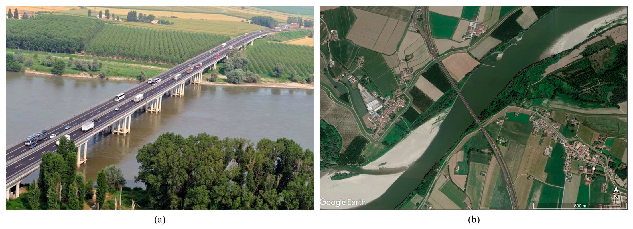
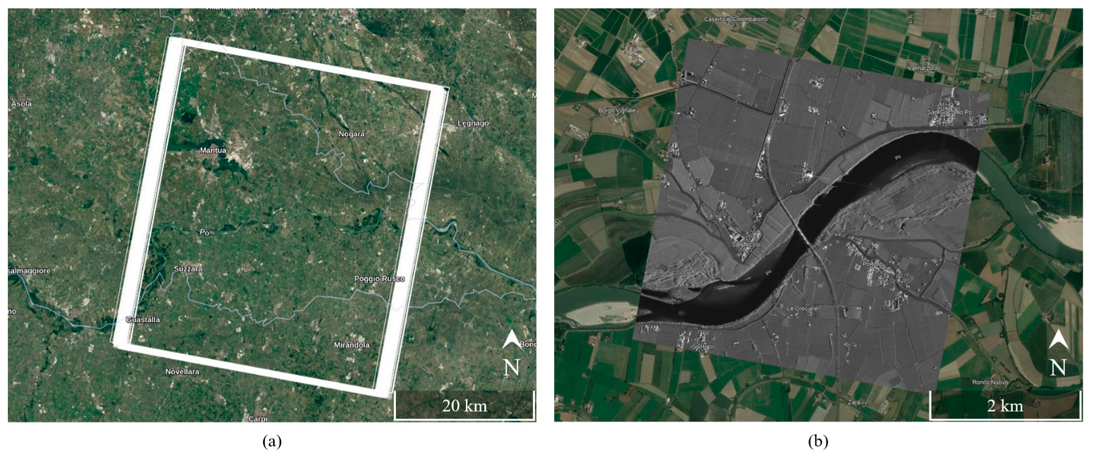
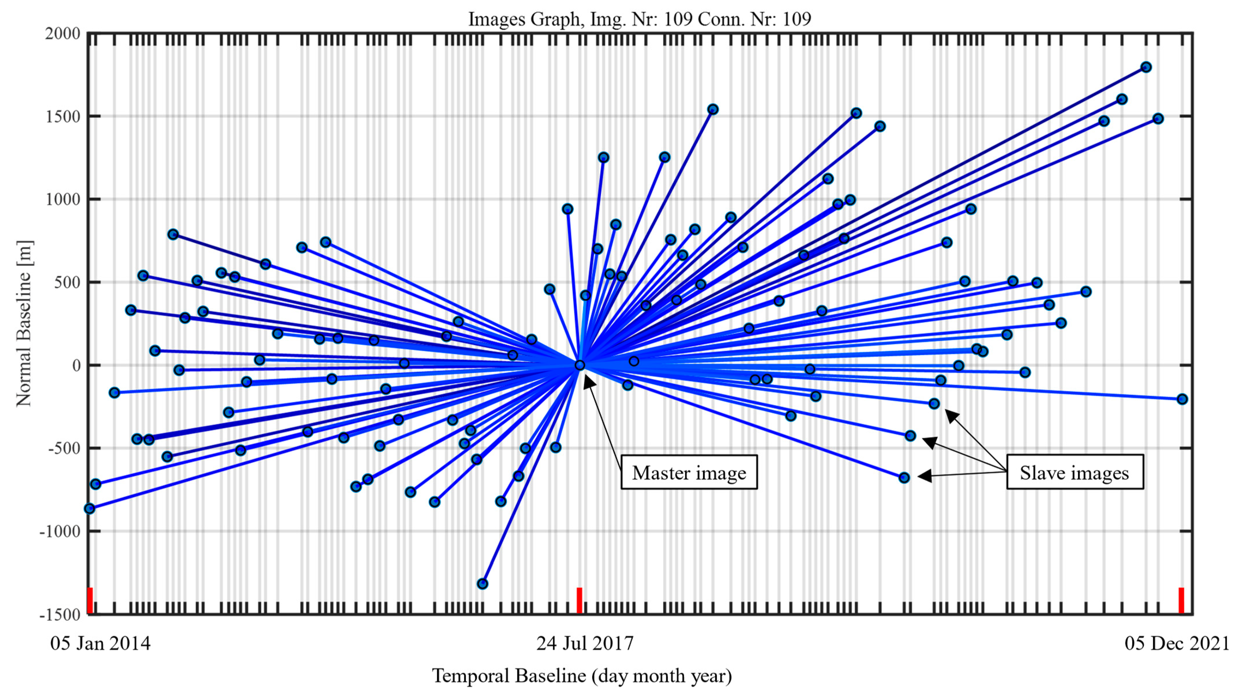
In the given context, this paper aims to cover the gap by presenting (i) an entire MT-InSAR data processing specifically performed for road bridges in operational conditions to extract displacement time series of PSs; (ii) the engineering interpretation of the millimetric ground and bridge displacements observed while being aware of the process followed to obtain such results; and (iii) a study of the correlation between the displacements of the bridge and environmental phenomena (temperature and river water flow) to further improve the engineering interpretation of InSAR results. Specifically, our analysis is based on a real-life case study: the A22 Po River Bridge of the Italian A22 Highway, a strategic, prestressed concrete bridge along the European route E45, which crosses the wider and longer Italian river, the Po River. Our study exploits a dataset of 109 X-Band HIMAGE mode Stripmap images acquired in the descending geometry by the Italian COSMO-SkyMed mission from 2014 to 2021. We performed the MT-InSAR data processing with the software SarProZ© (https://www.sarproz.com/), version ‘SARPROZ 08-September-2022 16:32:33’.
In detail, 
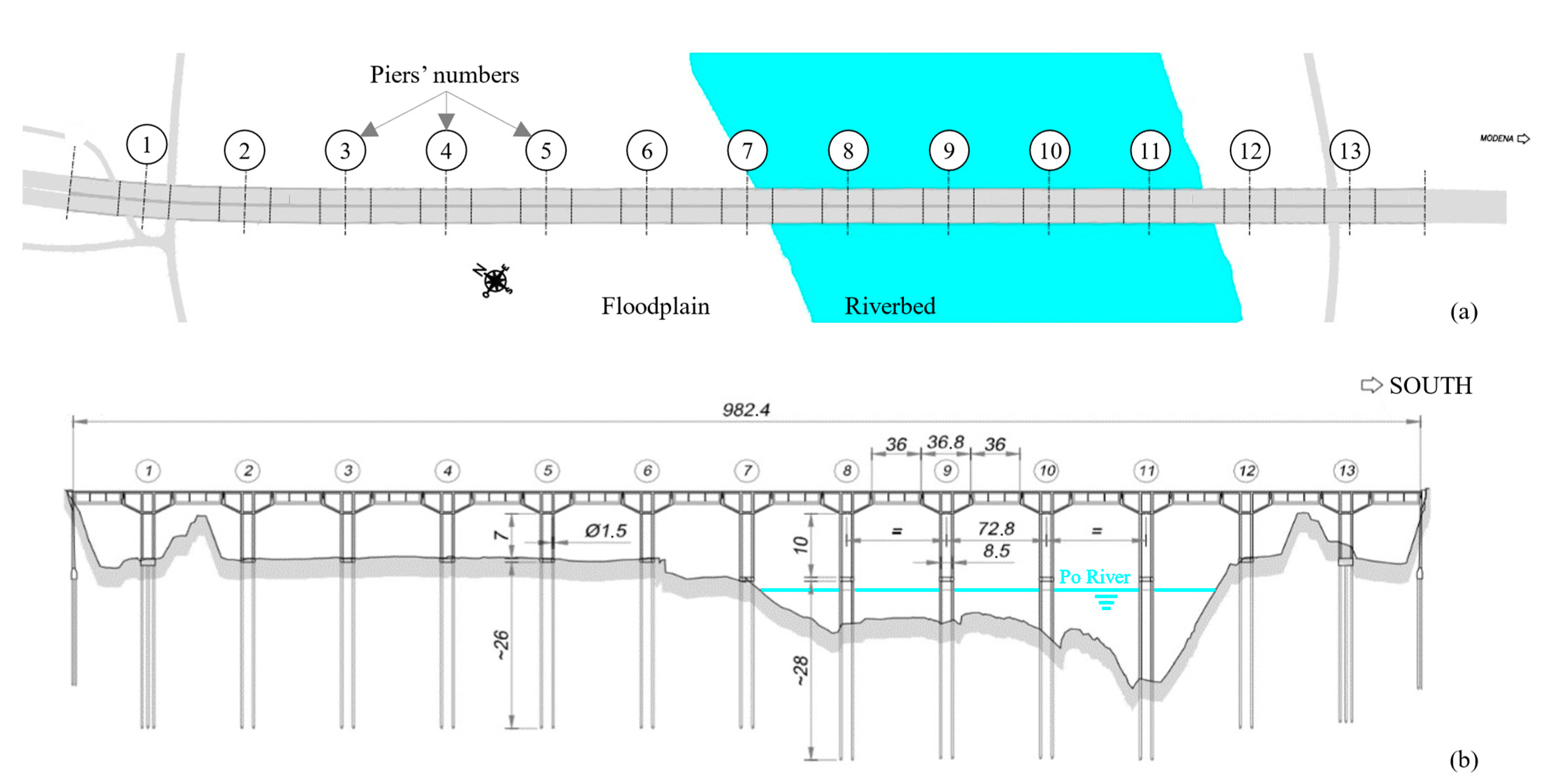
Section 2 introduces the A22 Po River Bridge, the case study area, and the dataset of SAR images. Section 3 describes the methods used to process SAR images through MT-InSAR, calculate the vertical and horizontal components of PSs displacements from the InSAR results, and study the correlation between the bridge displacements over time and the environmental load it experienced. Section 4 reports and discusses our study’s results, from the structural interpretation of the MT-InSAR displacements to the correlation analysis between bridge displacements and environmental loads. Conclusions are eventually drawn in Section 5.

2. Case Study

2.1. A22 Po River Bridge

The A22 Po River Bridge is part of the Italian A22 Highway. It is located in the Mantua province, Italy. It consists of two identical, parallel viaducts made entirely of reinforced concrete and prestressed concrete; it has 14 spans for a total length of 980 m. Each viaduct accommodates a separate highway carriageway. It was designed and built following the 1962 Italian standards for calculating loads of road bridges “Circ. Min. LL.PP. 14/02/1962, n. 384”. Figure 1 shows a picture of the A22 Po River Bridge and a top view of the case-study area. Figure 2 shows the plant and prospect of the bridge.
The structural system comprises 36 m-long internally simply supported spans that lean on shear keys at the end of 14.15 m-long cantilevers, resulting in a total span length of 72.8 m between the piers. The cantilevers’ deck comprises a double box girder with variable heights ranging from approximately 2.3 m to 3.5 m. The supported span girders are 2.2 m high. In 2002, a widening work involved the symmetrical widening of the carriageways from 10 m to 11.3 m, increasing the thickness of the upper slab. The original slab thickness ranged from 20–22 cm, which was increased to an average thickness of 35–37 cm for the suspended spans and piers. Additionally, the transverse slope of the deck was increased from the original 2% to the current 2.5%. Consequently, the widening works significantly increased the overall deck mass (approximately 6 t/m). Figure 3 shows longitudinal and cross sections of the bridge in the current configuration.
The suspended spans lean on monodirectional and multidirectional steel-Teflon bearings in the north direction and fixed steel bearings in the south direction. Seismic dissipators connect the suspended spans to the cantilevers at the shear keys with fixed bearings. Figure 4 shows a scheme of the suspended span bearings and a picture of the seismic dissipators.
The bridge has 13 piers, with 5 piers within the riverbed and 9 on the floodplain (6 on the north side towards Mantua and 2 on the south side towards Modena). Each pier consists of 6 circular column elements with a diameter of 1.5 m. At the base of the columns is a reinforced concrete collar with dimensions 2.0 m × 0.6 m. The foundation piles, also with a diameter of 1.5 m, extend below the collar and serve as natural extensions into the ground from the columns above. The piers in the riverbed have 10 m-heigh columns and approximately 28 m-long piles; the piers in the floodplain have 7 m-heigh columns and approximately 26 m-long piles.
The last bathymetric survey was performed in 2009, and backfill soil was placed around Pier 11 to decrease its free length in 2012. As a result, the above-ground part of the foundation poles is approximately 8 m for Piers 8, 9, and 10, approximately 11.40 m for Pier 11, and approximately 1 m for the other piers. The erosion at the base of Pier 11 was essentially caused by the increased speed of the stream and the formation of vortexes at the base of the pier; these actions generated the progressive removal of material (solid transport) in the area surrounding the base of the pier with the consequent formation of a localised depression in the riverbed. Given this erosion phenomenon, some backfill soil might have been removed since 2012.

2.2. Case Study Area and Environmental Loads

The case-study area is 17.6 km2, close to Mantua in northern Italy. It includes the villages of San Nicolò Po and Portiolo and is crossed by the Po River, Italy’s longest and widest river. This area is subjected to a slow progressive subsidence of around 1.0–1.5 mm/year, as visible in the vertical displacement measurement accessible from the European Ground Motion Service [26].
In the case study area, the subcontinental climate is characterised by high humidity, snowfall and fog in winter and a muggy, humid climate with little ventilation in summer. Temperatures vary between −5 °C and 40 °C throughout the year, with daily temperature variations of 10 °C to 15 °C around the average. Figure 5a shows the air temperature measured between UTC 5 p.m. and 5:30 p.m. from January 2014 to December 2021 by the meteorological station 5.6 km from the A22 Po River Bridge in Gorgo di San Benedetto Po (MN). As commonly known, the vertical deflection and longitudinal deformation of prestressed concrete bridges with a structural scheme similar to the A22 Po River Bridge strongly respond to temperature variation [27]. Thus, we expect to measure a periodical displacement of the A22 Po River Bridge from satellite SAR images, which is correlated to seasonal temperature variation.
Significant water flow variations characterise the Po River; the water level has periodically increased up to 10 m in the period we are interested in, which caused the floodplain to fill up during heavy rains. Figure 5b shows the water level of the Po River from 2014 to 2021 measured between UTC 5 p.m. and 5:30 p.m. by the hydrometer of the Interregional Agency for the River Po (AIPO) installed on the Borgoforte Bridge, located just 7.4 km before the A22 Po River Bridge.
The lithology of the foundation soils was deduced from the results of surveys conducted during the construction close to Pier 7 and the South Abutment. Surveys show a predominance of uniform grain size sands with traces of silt in the higher levels and peaty traces at the deeper levels (>15 m from ground level). The survey report indicates an average value of the soil elastic modulus of 8 MPa, constant over a depth of 15 m from ground level, and a friction angle conservatively assumed to be φ = 32° at the base of the piles and zero cohesion over the entire length of the foundation piles.

2.3. Dataset of SAR Images

We analysed a dataset of SAR images acquired by the Italian satellite mission COSMO-SkyMed (CSK, 1st generation), which have been granted free of charge by the Italian Space Agency (ASI) to the Department of Civil, Environmental and Mechanical Engineering at the University of Trento. CSK satellites carry X-band radar sensors with a frequency of 9.6 GHz and a wavelength of 3.1 cm. The revisit time of the CSK constellation (i.e., the number of days between two successive identical passes over the same area) is about 16 days; therefore, the temporal resolution is about 1–2 products per month for images of the same area in both ascending and descending geometry.
Our dataset includes CSK images acquired in Stripmap HIMAGE mode—a medium-resolution mode with a nominal spatial resolution of 3 m—collected over long, continuous 40 km-wide swaths. The dataset counts 109 images acquired in descending orbit at UTC 5:13 p.m. and covers 8 years, from 1 May 2014 to 12 May 2021. The CSK satellite that acquired the images of our dataset has right-side looking-angle with an incidence angle θ = 33.9449° (i.e., the angle between the LoS and the normal to the ground in our area) and a heading angle β = 10.6095° (i.e., the angle between the satellite orbit and the North-South direction). Figure 6a shows the footprint of our dataset. The investigated area is a 4.2 × 4.2 km2 portion of this footprint, cropped from the original SAR images and shown in Figure 6b. It includes the A22 Po River Bridge and the villages of San Nicolò Po and Portiolo. Villages and artificial structures in this area contribute to the successful co-registration of SAR imagery. Figure 7 shows the “Star Graph” connecting the dataset, highlighting the temporal and normal baselines. The master image of the descending dataset corresponds to the date 24 July 2017; it is the barycentre of the images’ graph and minimises the temporal and normal baselines, reducing the temporal and spatial decorrelation between images.

3. Method

3.1. Multi-Temporal InSAR for Bridge Monitoring

InSAR is a remote sensing technique that uses the phase information of radar signals emitted by Synthetic Aperture Radar (SAR) sensors mounted on satellites and backscattered by the Earth’s surface to measure the displacement of reflective targets along the Line of Sight (LoS) of the satellites [28]. A SAR image is a collection of complex numbers organised in pixels over the investigated portion of the Earth’s surface. The module of the complex number represents the signal amplitude and is related to the target reflectivity; the phase of the complex number is related to the distance between the radar sensor and the reflective target in the pixel. By comparing two or more SAR images of the same area taken at different times (repeat-pass interferometry), it is possible to calculate the phase differences of pixels between the images, which are related to the deformation of the Earth’s surface. The phase differences can be converted into a displacement map showing the spatial distribution of the reflective targets’ displacements along the LoS. Those reflective targets are called Scatterers (PSs) and are point-like targets that exhibit high reflectivity and stable phase behaviour over time).
The standard InSAR approach is affected by many different limitations, so different Multi-Temporal InSAR (MT-InSAR) techniques have been developed in the last decades [8,9,10,15]. The MT-InSAR technique is a method of processing SAR images that allows for detecting small changes in the Earth’s surface over long periods. This technique involves analysing a series of radar images of the same area taken over several years and comparing the phase differences between them and a reference image called master.
After the coregistration of all 109 SAR images and the preliminary analysis aimed at deriving the dataset’s main statistics, we performed the actual MT-InSAR processing. The following are the main steps involved in our MT-InSAR workflow and the main choices we made during the analysis of our dataset:
(1)
Atmospheric-phase removal. One advantage of MT-InSAR compared to standard InSAR is the possibility to estimate and remove the atmospheric phase disturbance from the SAR images. This step is critical because the atmospheric phase contribution is one of the primary sources of error in InSAR data. An initial selection of pixels related to potential candidate targets (the PSs) is processed by connecting them in a spatial graph and estimating the main parameters affecting the interferometric phase along the connections (for our case, deformation velocity, thermal expansion, and height of the targets). After this estimation, the residual phase signal is used to estimate and remove the Atmospheric Phase Screen (APS) contribution from the original SAR images [28].
(2)
Persistent Scatterer Selection. Once the APS phase contribution is removed from the images, a higher number of pixels can be analysed with the MT-InSAR algorithm to derive the parameters with respect to a common reference point (RP)—a specific PS used to anchor the estimated deformation time series. The RP is selected based on high temporal coherence and limited deformation over time [15,28]. After estimating the parameters, we filtered out all PSs with a temporal coherence lower than 0.6. We recall that temporal coherence is a quality metric of the extracted displacement time series with respect to the model used and ranges from 0 (low quality) to 1 (high quality) [28]. As a result, we included 8426 PSs in our analysis, most of them located over roads and villages.
(3)
Time series analysis. Deformation time series can be extracted for every PSs based on the filtered phase data. Displacements are relative in time and space. In time, they are relative to the date of the master image; in space, they are relative to the displacement of the common RP (the same used in the previous step of the analysis). Note that deformations mean displacements along the Line of Sight of the satellite. A negative deformation means that the PS moves away from the satellite, while a positive deformation means that the PS moves towards the satellite.
Figure 8 shows some results obtained during the MT-InSAR data processing of our dataset.

3.2. Calculation of Vertical and Horizontal Displacement

Suppose the displacements of an area of the Earth’s surface along the LoS of satellites within a specific time interval are known for ascending and descending geometries. In that case, it is possible to derive the East–West and vertical displacements of the PSs in the same area using trigonometric calculations that depend solely on the incidence angles of the two geometries. More information on the assumptions and the procedure to perform this calculation can be found in [29]. In our study, we only analysed SAR images acquired in the descending geometry because the dataset of SAR images acquired in the ascending geometry is highly incomplete. Therefore, we cannot utilise the procedure mentioned above to extract the vertical and horizontal displacements of the bridge. However, we can study the bridge behaviour under the two extreme conditions: (i) the deck experiences exclusively vertical displacements, and (ii) the deck experiences exclusively horizontal displacements while being aware that the actual behaviour of the bridge is a combination of these two.
In the case of these two extreme conditions, it is possible to project the measured PS displacements along the LoS (dLoS) onto the vertical (dV) and horizontal (dH) components of the LoS, given the incidence angle of the LoS, which is θ = 33.9449° for our dataset. Furthermore, in the case of exclusively horizontal displacements along the longitudinal direction of the bridge, it is possible to project horizontal displacements dH onto the longitudinal direction of the bridge (dL), knowing the angle between the satellite’s orbit direction and the North–South direction (heading angle, β = 10.6095°) and the angle between the bridge’s direction and the North–South direction (bridge orientation, ζ = −33.5°). Figure 9 shows these projections for displacements derived from a right-looking satellite in descending geometry and for the actual orientation of the Po River Bridge.
Although strong, the hypothesis of exclusively longitudinal horizontal displacements is plausible for the Po River Bridge portion in the floodplain, as no loads induce transversal displacements to the bridge’s direction. Indeed, displacements induced by wind have a frequency and variability too high to be observed with the 16-day acquisition frequency determined by the satellite’s revisit time. The only displacements induced by environmental loads observable on this bridge portion at this acquisition frequency are those resulting from seasonal temperature variations. A different scenario applies to the displacements of the bridge portion in the riverbed, which can also be influenced by the hydraulic forces of the Po River on the piers, transverse to the bridge’s direction, varying with changes in the water level measured by the hydrometer located upstream of the bridge.
Regarding our dataset, the CSK satellite that acquired the SAR images moved from North to South with a right-looking angle. Considering that a negative deformation means that the PS moves away from the satellite, while a positive deformation means that the PS moves towards the satellite, we can conclude that:
  • Negative displacement along the LoS of a PS means that that portion of the bridge moves mainly vertically downward, mainly horizontally toward the West, or a combination of the two;
  • Positive displacement along the LoS of a PS means that that portion of the bridge moves mainly vertically upwards or mainly horizontally toward the East, or a combination of the two.

3.3. Correlation between Time Series

Displacements of isostatic structures are typically linearly correlated to the loads applied (e.g., dead loads, live loads, and temperature variations). Many studies investigate the correlation between time series of environmental loads and measurements from long-term monitoring of civil structures [30]. Correlation analysis is a method of statistical evaluation used to study the strength of a relationship between continuous variables. Given two random variables, X and Y, the Pearson correlation coefficient ρXY expresses their linear correlation [31]. The Pearson coefficient ranges between −1 and +1: +1 means perfect direct correlation, and −1 means perfect inverse correlation. Investigating a potential correlation between variables employing the Pearson coefficient involves considering the hypothesis of a linear relationship between them. However, it should be acknowledged that variables can exhibit more complex relationships than simple linear ones. Remarkably, two datasets with low or no linear correlation may demonstrate a robust nonlinear relationship. Nevertheless, assessing linear correlation as a preliminary step is valuable for identifying variables that exhibit a relationship before performing further correlation analyses.

4. Results and Discussion

Section 4.1 and Section 4.2 report and discuss the results directly obtained from the MT-InSAR analysis of COSMO-SkyMed SAR images of the area of interest. Specifically, Section 4.1 interprets the displacement time series and velocity of the PSs identified on the bridge and its access lines, while Section 4.2 interprets their consistency with the expected response to temperature variation. On the other hand, Section 4.3 and Section 4.4 investigate and discuss the correlation between the displacement time series and environmental loads. Specifically, Section 4.3 focuses on the correlation of displacements with the variations in air temperature, while Section 4.4 focuses on the correlation of displacements with the variation of the water level of the Po River measured in proximity to the bridge. They also investigate whether it is possible to identify different bridge spans based on the opposite longitudinal deformation of the bridge cantilevers in the floodplain and the effect of water level variation on the response of the bridge piers in the riverbed.

4.1. Structural Interpretation of PS Deformation Velocity

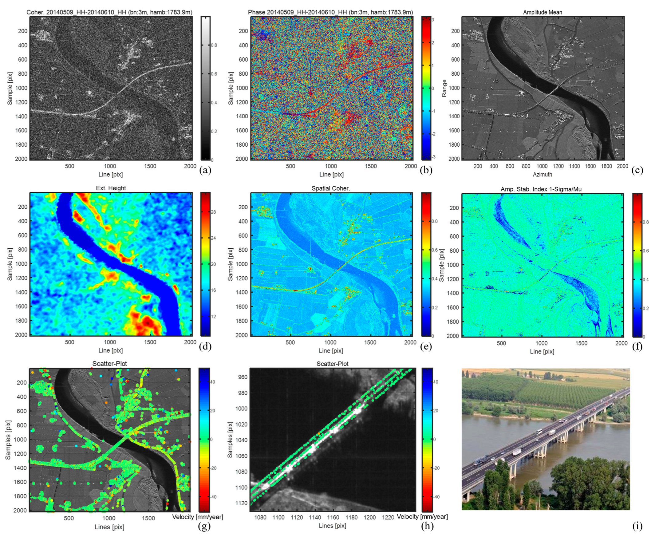
Using the MT-InSAR technique, we identified 8426 PSs on the bridge and in its surrounding area, and we extracted the time series of displacements along the LoS over eight years, from 2014 to 2021. 
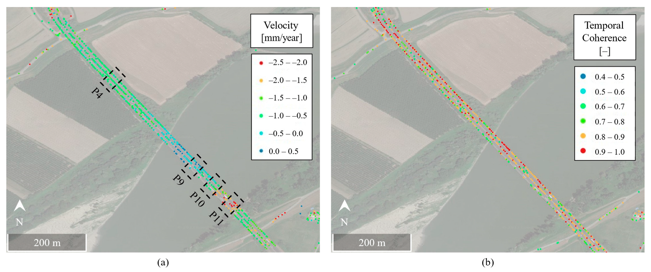
Figure 10 shows the PSs’ distribution in the case-study area, illustrated in a colour scale representing their displacement velocity along the satellite LoS. The velocity ranges from −13.21 mm/year (away from the satellite, in red) to 3.59 mm/year (toward the satellite, in blue). The velocity of PSs has been calculated during the MT-InSAR data processing by fitting a linear function over the entire time series of displacement through the least-square analysis. The standard deviations of the estimated velocity range between 0.21 and 0.56 mm/year, depending on the considered PS.
The PSs are mainly concentrated along the highway, within urban centres, and along local roads. As expected, the PSs are absent along the river and cultivated fields, except for four aligned PSs in the upper left corner, corresponding to high-voltage power line towers. Most PSs are coloured in green, indicating nearly negligible deformation velocity ranging between −1.5 and +1.5 mm/year. The road accessing the bridge from the south exhibits red and orange PSs, as does the road adjacent to the southern embankment of the river. The bridge is primarily covered by green PSs, with a small yellow portion—meaning deformation velocity between −3 and −1.5 mm/year—near Piers 10 and 11. These results suggest that the bridge experiences nearly negligible deformation velocity throughout its span, except for the portion that underwent significant erosion at the base of the piers and was retrofitted with backfill soil in 2012, as indicated by the yellow colour of PSs. This result may suggest the resumption of erosion phenomena at the base of the piers, which may have eroded the backfill soil after 2012.
It is important to note that the deformation measurements obtained using the MT-InSAR technique from SAR satellite images are along the satellite LoS, i.e., from the sky to the ground and from right to left in this image. Negative values indicate displacements away from the satellite; therefore, negative velocities may result from a combination of downward and westward displacements.
We focus on the deformation velocities ranging from 0.5 to −2.5 mm/year to investigate the bridge displacements further; this allows for a better graphical representation—with greater details—of the PS displacements extracted along the bridge’s LoS. Figure 11a shows the PSs on the bridge in a colour scale representing velocity with small ranges; Figure 11b shows the same PSs in a colour scale representing temporal coherence; as we can see, the temporal coherence of these PSs is mostly higher than 0.7, confirming the results’ quality.
Let us focus on Figure 11a. In the portion of the bridge over the floodplain, the deformation velocities are mainly between −0.5 and −1 mm/year. Conversely, in the portion of the bridge over the riverbed, the deformation velocities are close to 0 mm/year towards the north bank of the river and exceed −2 mm/year near Piers 10 and 11. The velocities return to approximately −0.5 mm/year after leaving the river’s south bank. This result confirms the nearly negligible deformation velocity along most of the bridge but close to Piers 10 and 11.

4.2. Structural Interpretation of PS Deformation Periodicity

Besides studying the deformation velocities of the different bridge sections and the surrounding territory, we are interested in investigating the periodicity of the observed displacements because we expect their correlation with the seasonal air temperature variations in that area. For this purpose, in Figure 12 and Figure 13, we isolated the displacement time series of some PSs of particular interest to observe and discuss them. All the selected PSs have temporal coherence higher than 0.8.
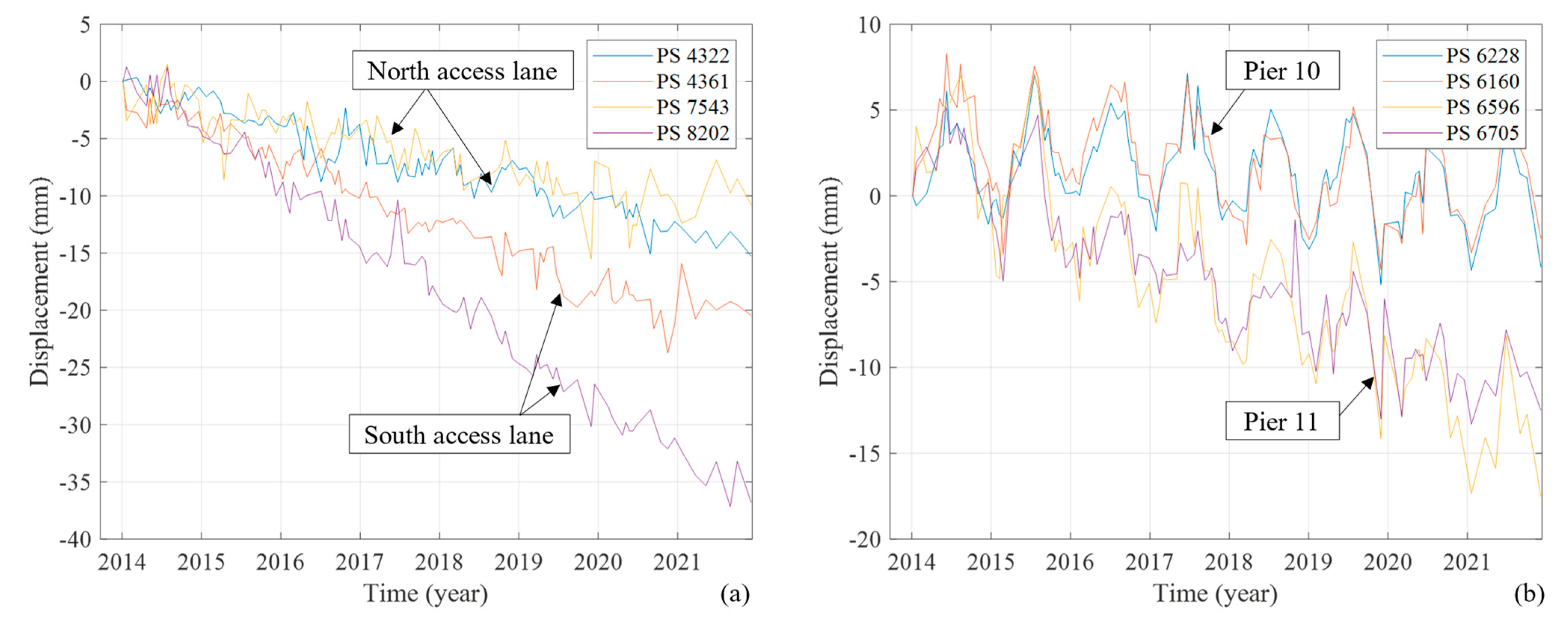
Let us begin with the PSs located on the access lane north and south of the viaduct, whose displacement time series are shown in Figure 12a. We can observe that the displacement time series of a PS on the southern access lane (PS 8202) is characterised by a deformation velocity exceeding −5 mm/year along the LoS and limited seasonal periodicity. The limited periodicity aligns with the expectation since this access lane has been constructed with embankment soil, which is not expected to exhibit significant displacements in response to temperature variations. In contrast, the high velocity suggests abnormal displacements of the access lane. The infrastructure operator has recently detected such abnormal displacements and is already addressing this issue. A similar behaviour is observed on the northern access lane, where the periodicity is almost absent, and the deformation velocity is around −2 mm/year, indicating a less pronounced effect than the southern access lane, consistent with the results shown in Figure 10.
Next, we examine the displacement time series of some PSs identified along the bridge. Figure 12b illustrates the displacements of the top of Piers 10 and 11, represented by yellow PSs in Figure 10. It is evident that the behaviour is similar for both PSs: a noticeable negative displacement trend along the LoS of approximately −2 mm/year—even though more pronounced in the PSs located at the top of Pier 11—and a more visible periodicity compared to the PSs on the access lanes.
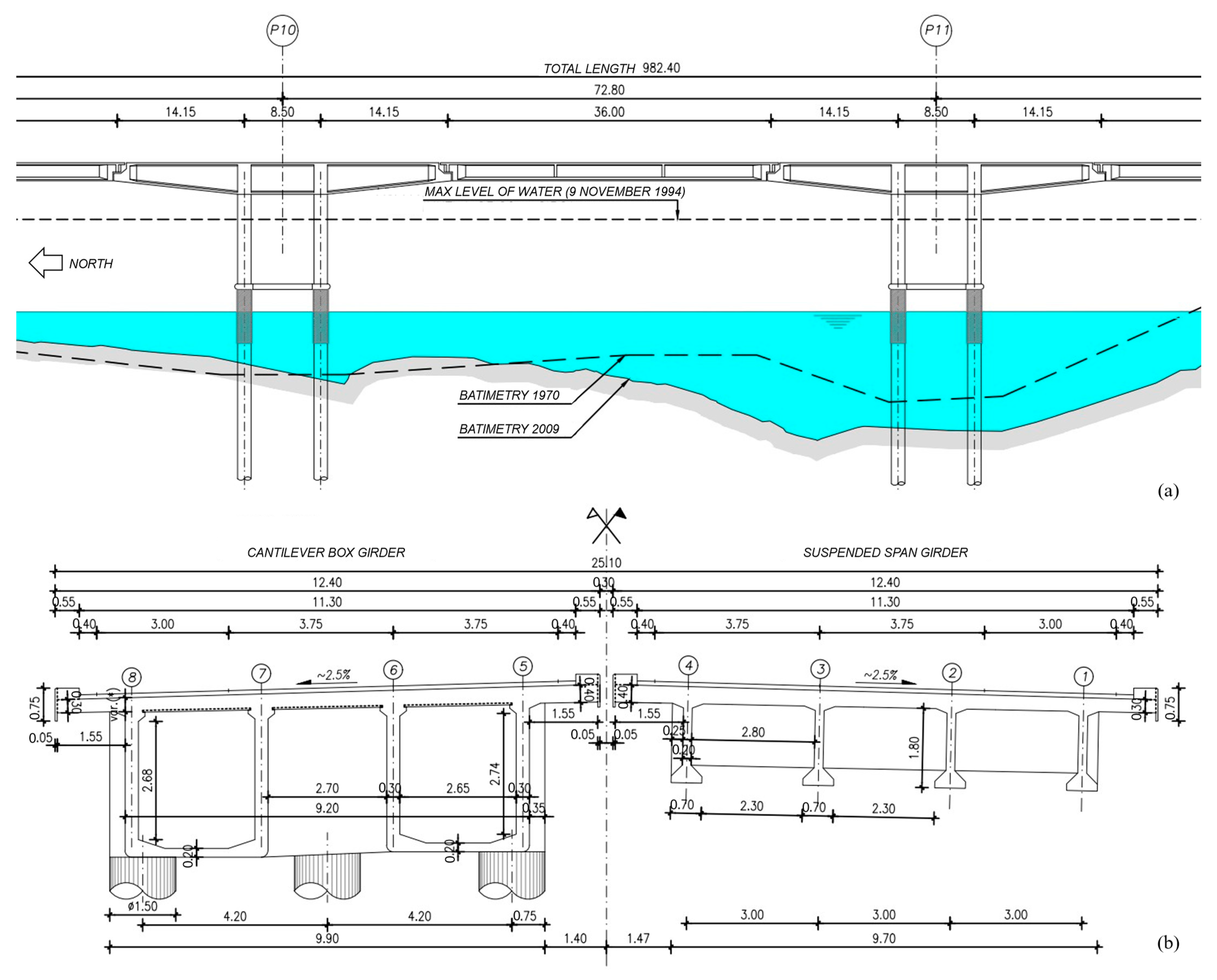
The greater periodicity was expected since these are displacements of reinforced concrete piers with a theoretical thermal expansion coefficient of around α = 15 10−6 °C−1. We can estimate the actual thermal expansion coefficient α based on the observed displacements and the measured temperatures. That would allow us to qualitatively verify whether the displacements obtained through MT-InSAR applied to our dataset are consistent with the expected displacements for a structure of this type. To do this, we perform the following procedure, whose results are reported in Table 1:
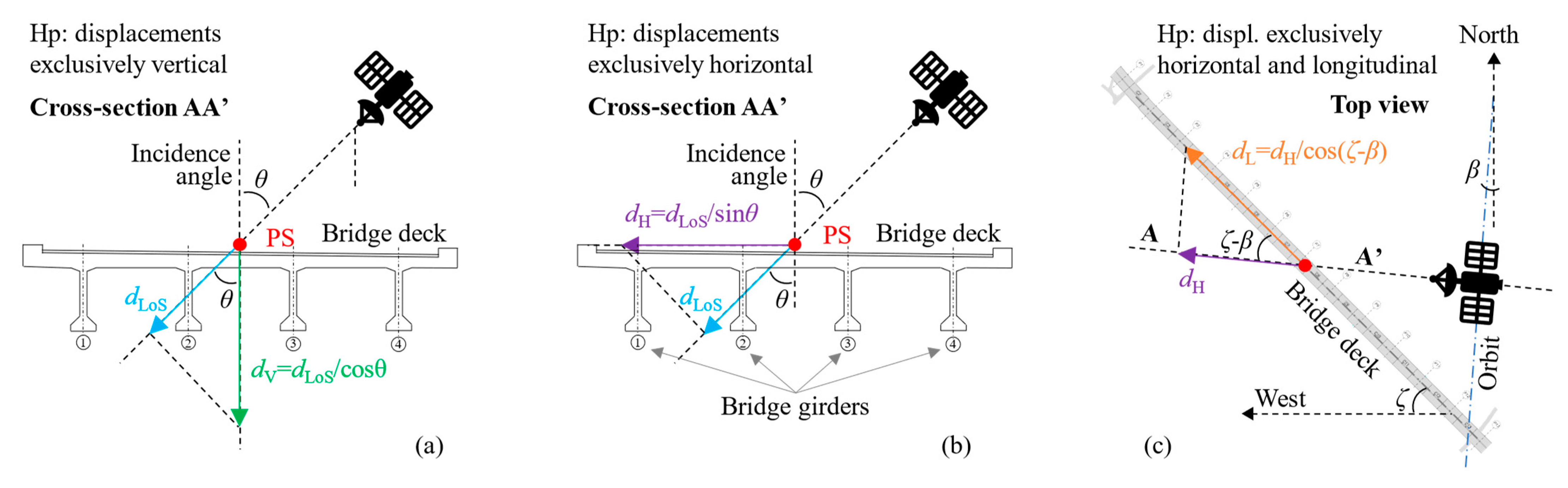
  • Assume that the piers’ displacements in response to thermal variations are mainly vertical;
  • Project the observed displacements along the LoS (dLoS) onto the vertical direction (dV) according to Equation (1), knowing the incidence angle θ = 33.9449°:
    dV = dLoS/cosθ
  • Divide the vertical displacements by the height of the piers and the girders (approximately 15 m above the river surface) to obtain the time series of vertical deformation ε of Piers 10 and 11;
  • Fit the time series of vertical displacement with Least Square Analysis (LSA) and a linear model that takes as inputs deformations ε, temperatures T, and the time t at which the measurements were taken and estimates a purely geometric offset ε0, the deformation trend v, and the thermal deformation coefficient α. The model is described in Equation (2):
    ε = ε0 + v t + α T
The velocities—v [mm/year]—are consistent with those obtained directly from the MT-InSAR analysis (see Figure 12b), and the thermal expansion coefficients α are consistent with those expected for prestressed concrete bridges. These results allow us to conclude that the magnitude of the periodic displacements observed through this technique is consistent with the expected temperature response for this bridge.
Now, let us focus on the part of the bridge characterised by green PSs in Figure 10 and Figure 11, indicating deformation velocities between −1.5 and 1.5 mm/year. Figure 13a,b show the displacements of the north and south cantilevers of Pier 4 in the floodplain, while Figure 13c,d show the displacements of the north and south cantilevers of Pier 9 in the riverbed. We can observe that all displacement time series exhibit a significant periodicity with an annual period, consistent with the periodicity of temperature variations. However, there is an opposite sign in the displacement variation between the PSs in opposite cantilevers of Pier 4: when the northern cantilever displacements increase, the southern cantilever displacements decrease, and vice versa. Regarding the observed displacements of the cantilever of the riverbed Pier 9, periodicity is present but less pronounced on the northern side than on the southern side. However, unlike Pier 4, where a deflection trend is clearly visible, displacements of Pier 9 seem to be affected by other phenomena in addition to temperature variation. We will discuss this in Section 4.4.

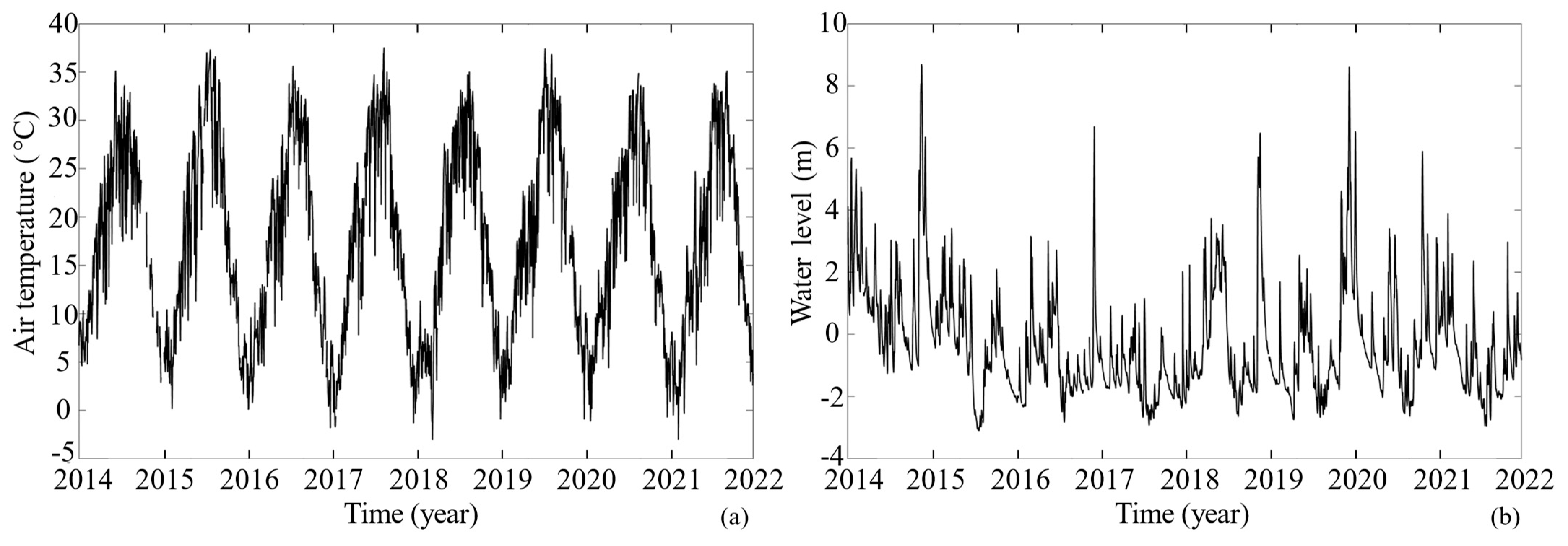
4.3. Correlation between Displacements and Temperature Variations

We start the correlation analysis by studying the linear correlation between PS displacements and temperature variations. First, we decimate the temperature dataset to one measurement per day for the days corresponding to the satellite passage over the case study area.
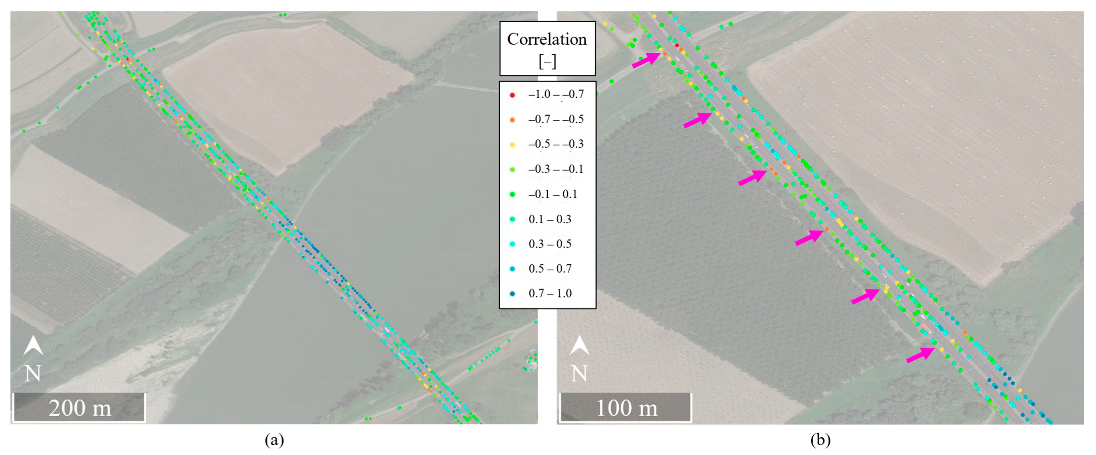
Figure 14 illustrates the map of identified PSs on the bridge, represented in a colour scale corresponding to the Pearson correlation coefficient resulting from comparing displacements time series of each PS and temperatures. In Figure 14a, we can immediately observe a clear difference in correlation values between the floodplain and the riverbed portions. Specifically, a positive correlation ranging from 1 to 0.7 is observed in the riverbed portion between Piers 8 and 11, while a positive but lower correlation—below 0.5—is seen between Pier 11 and the southern bank of the river. In contrast, in the floodplain portion, there is a periodic variation in the colours of the PSs, ranging from transverse groups of yellow–orange–red PSs (with a negative correlation between −1 and −0.3) to transverse groups of green PSs (with a correlation between −0.3 and 0.1), and finally to transverse groups of blue PSs (with a correlation between 0.1 and 0.5), followed by another yellow–red PS groups (where the correlation drops down to −1 again). Figure 14b shows a zoom on the floodplain portion of the bridge where magenta arrows highlight the yellow–red coloured PS groups.
These differences in the linear correlation are also clearly visible in 
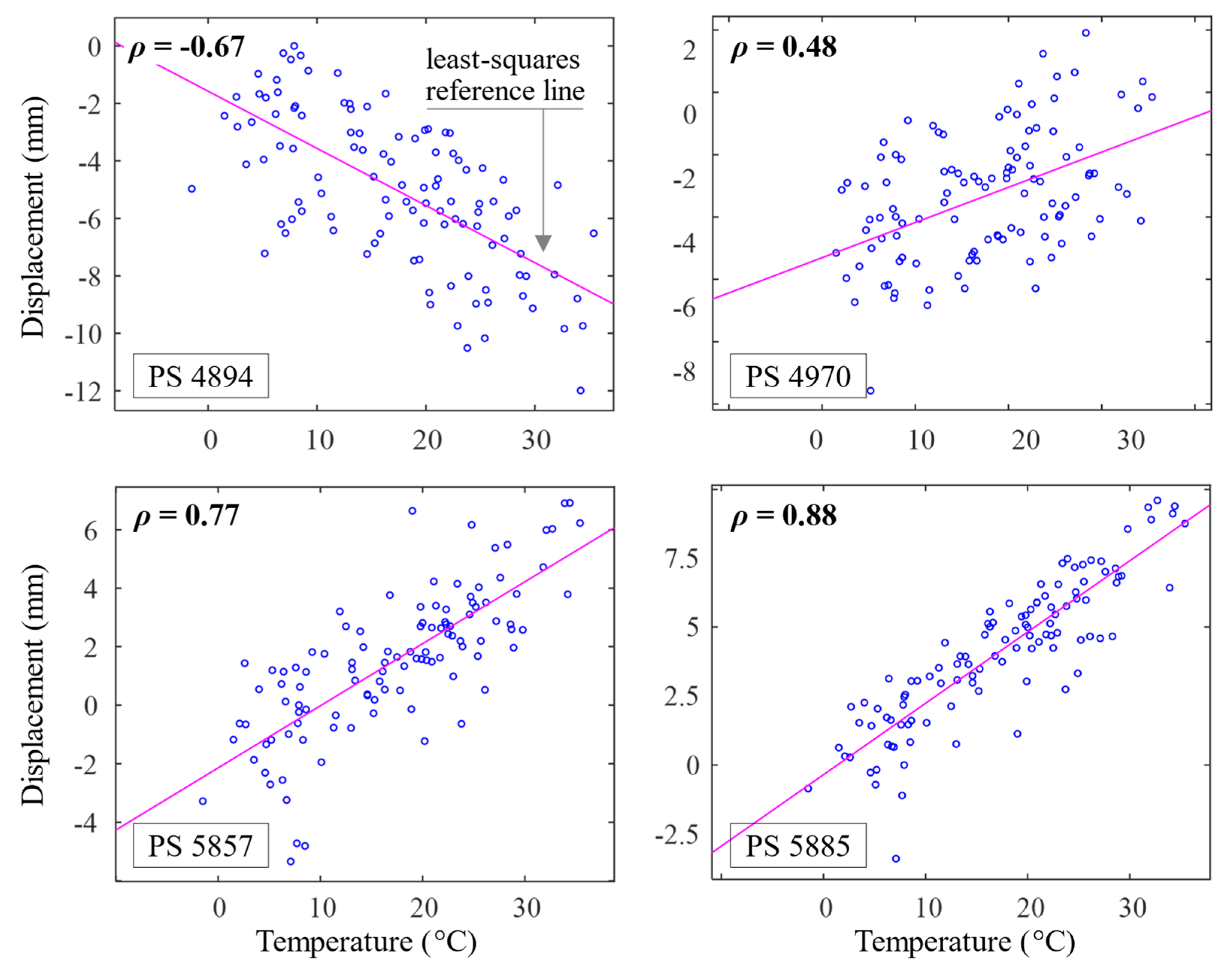
Figure 15, which shows the scatterplot of the variables Displacements (dLoS) and Temperature with the least-squares reference line—the slope of which is equal to the displayed correlation coefficient ρ—for some PSs whose displacement time series have been reported in Figure 13. In the riverbed, the displacements of the PSs located over the Pier 9 exhibit a positive correlation ranging from 0.7 to 0.9. In the floodplain, the displacements of the PSs located over the north cantilever of Pier 4 exhibit a negative correlation, while those located over its south cantilever exhibit a positive correlation.
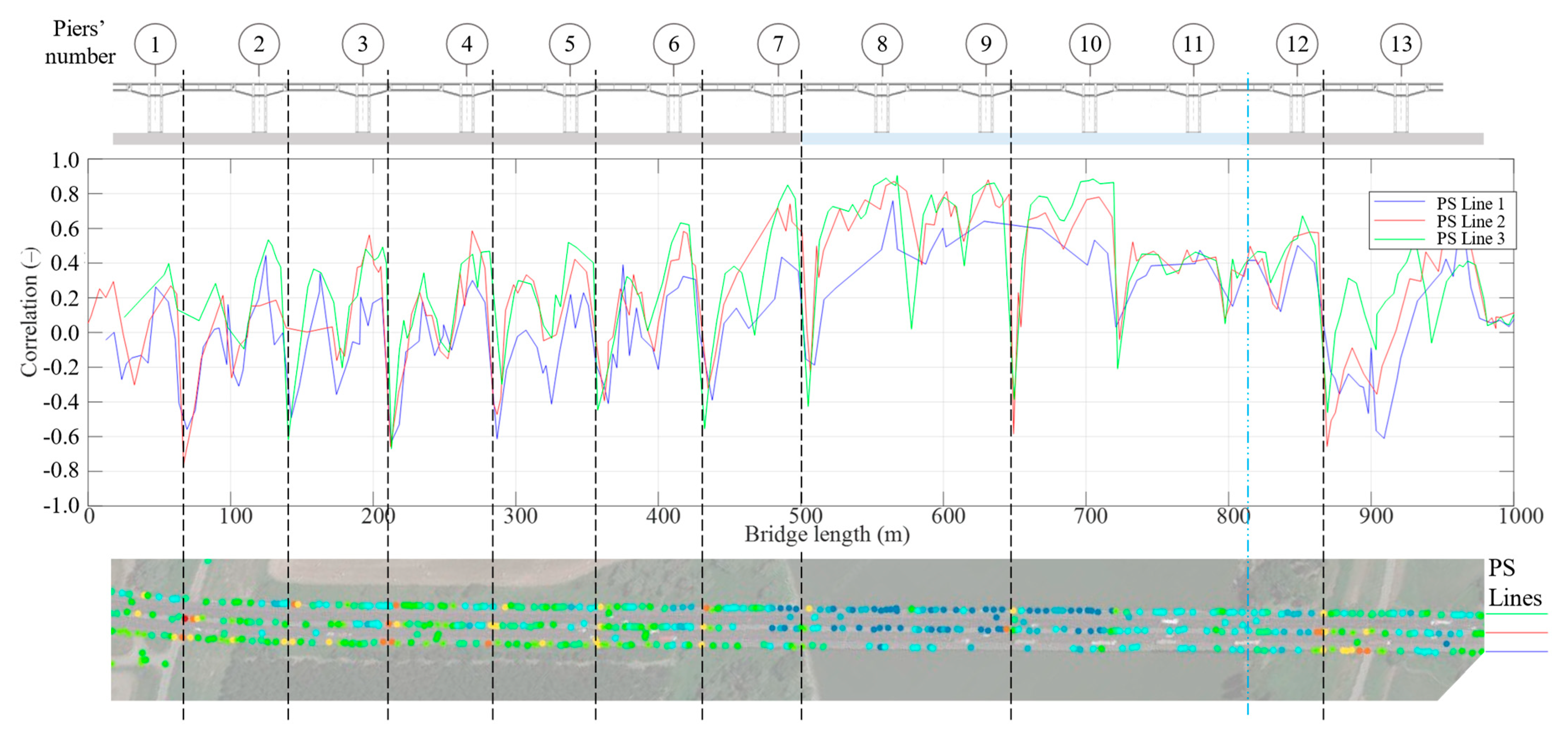
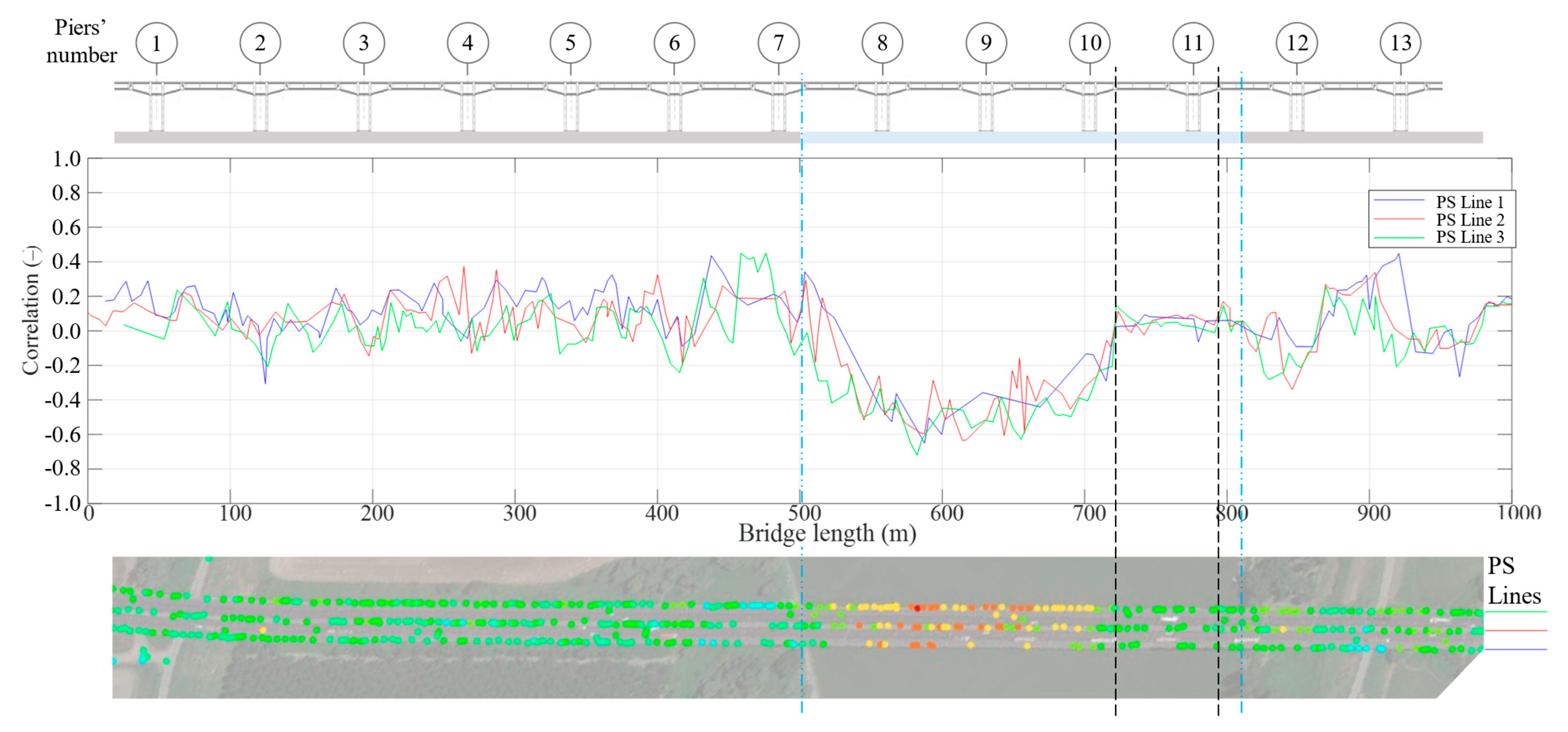
This periodic variation of the linear correlation along the bridge is clearly visible in Figure 16, where this parameter is reported for the three lines of PSs highlighted in the figure plotted against the length of the bridge. Figure 16 also shows the longitudinal section of the bridge on the same scale as the PS map and the graph. Marking the negative peaks of the correlation (see the black dashed lines in 
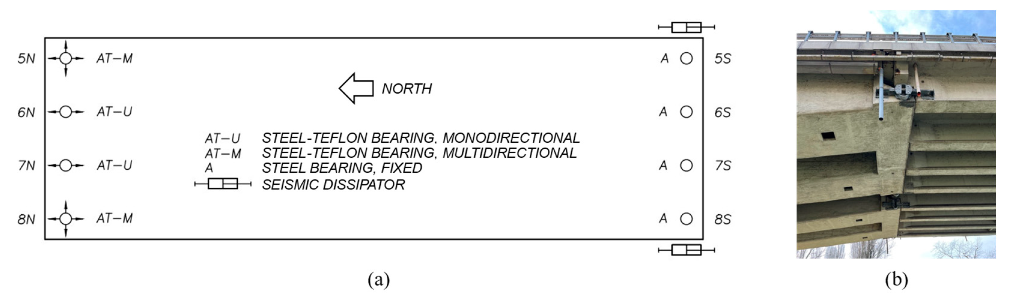
Figure 16), we can notice that they correspond to the right (northern) joint of the suspended span—the one with monodirectional and multidirectional bearing (thus, roller supports).
To confirm the periodicity in the correlation variation along the bridge length observed in Figure 14 and Figure 16, we fitted the three PS lines highlighted in Figure 16 with the sine function A·sin(ω·x + φ), where A, ω, and φ are free parameters, and x is the longitudinal coordinate along the bridge. The estimated parameters are reported in Table 2, along with the estimated periodicity T = 2π/ω. The estimated periodicity results between 72.72 m and 73.15 m, almost equal to the spacing of the spans (72.80 m, see Figure 3), and thus the distance between two consecutive roller supports.
This result is in line with the expected longitudinal response of the bridge deck to temperature variation: the longitudinal displacements are zero over the piers and increase along the cantilevers until the joints as we move away from the piers; the suspended spans move longitudinally in the direction of the cantilever which supports it with fixed bearings. The possibility of noticing it with such clarity from satellite measurements is quite sensational.
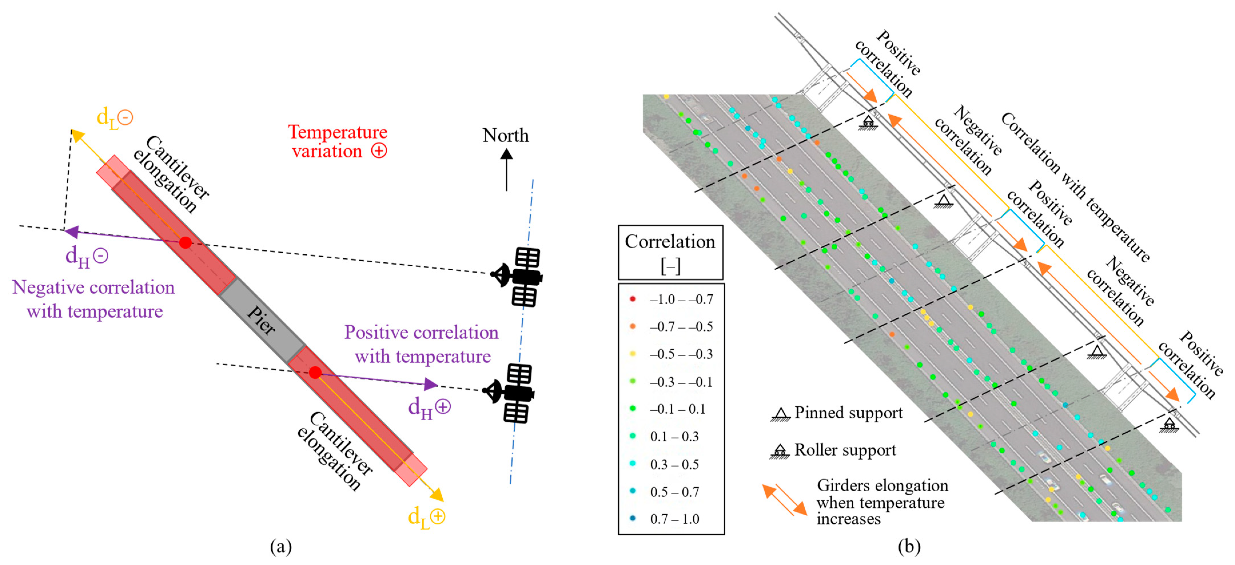
Let us discuss more in-depth why we can observe such periodic correlation. As shown in Figure 17a, the correlation is negative in the northern portion of the pier as the longitudinal displacements have an opposite sign to the temperature variation. Conversely, the correlation is positive in the southern portion of the pier as displacements and temperature variations share the same sign. Figure 17b illustrates this result with the correlations obtained for the A22 Po River Bridge. This result allows us to conclude that, for the A22 Po River Bridge, the horizontal longitudinal displacements in response to temperature variation can be clearly observed with satellite InSAR-based SHM. Moreover, and most importantly, it is possible to identify different spans of the bridge simply by studying the sign of the correlation between displacement and temperature variation and its periodicity along the length of the bridge. This finding is quite important in view of using this type of monitoring to detect anomalous bridge behaviour on a large scale automatically.
Regarding displacements in the riverbed, a certain periodicity in the colours of the PSs is maintained, suggesting that the observations made for the floodplain portion can be extended, even though in a purely qualitative manner, to the riverbed portion.

4.4. Correlation between Displacements and Water Level Variations

We proceed with the correlation analysis by studying the correlation between PS displacements and water level variations of the Po River. First, we decimate the water level dataset to one measurement per day for the days corresponding to the satellite passage over the case study area.
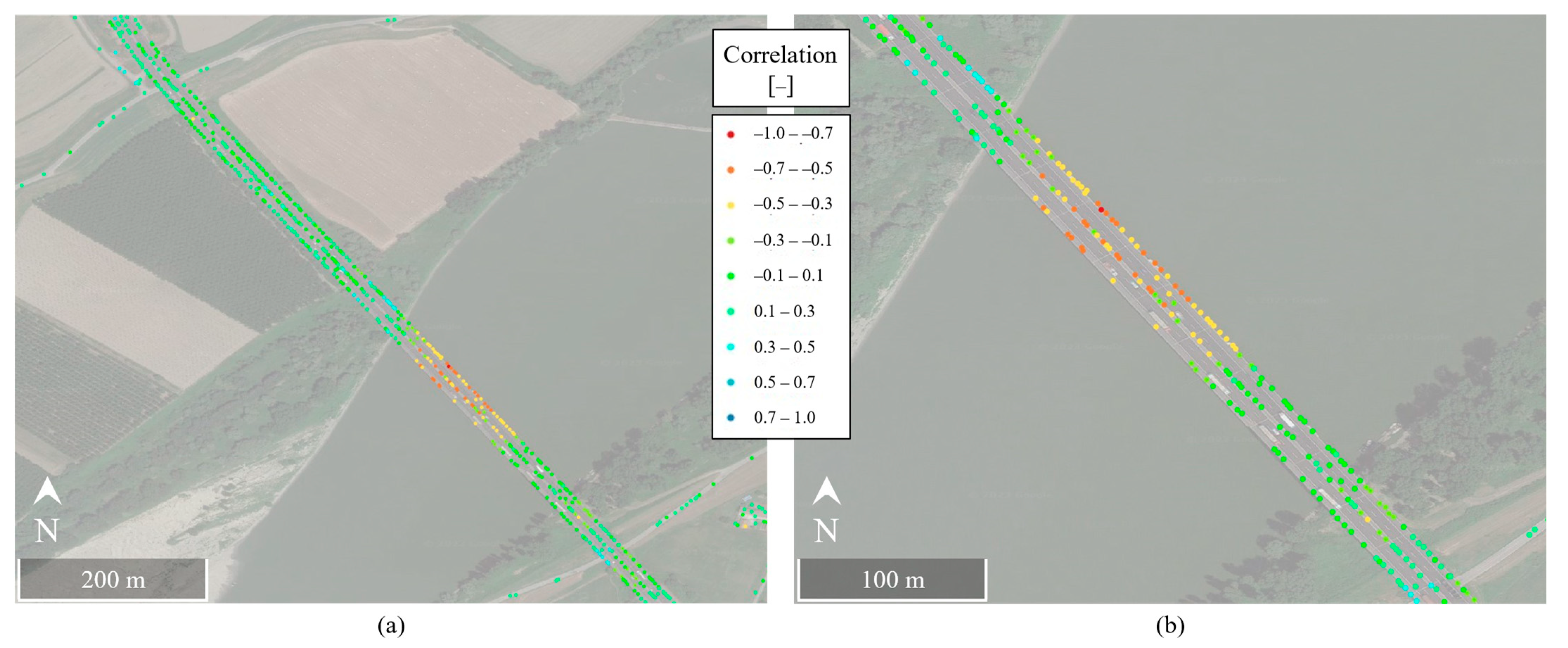
Figure 18a illustrates the map of the identified PS on the bridge, represented in a colour scale corresponding to the Pearson correlation coefficient resulting from comparing displacements and water level for each PS. Figure 18b shows a zoom on the riverbed portion of the bridge.
As in Figure 14a, we can observe in Figure 18a a clear difference in the correlation values between the floodplain and the riverbed portions. Specifically, we notice that the Pearson coefficient of most PSs in the floodplain portion of the bridge is almost zero, while it is negative and between −0.5 and −1 for the PSs over the riverbed portion. This difference in correlation along the bridge is also clearly visible in Figure 19, where this parameter is reported for the three lines of PSs highlighted in the figure plotted against the length of the bridge.
The displacement periodicity of the PSs in the floodplain does not seem correlated with the seasonal water level changes. In contrast, the displacement periodicity of the PSs in the riverbed does, with downward-westward displacements occurring when the water level rises—the Po River flows from West to East. Since the soil is highly heterogeneous, these displacements may be related to ground deformations associated with seepage through soils of different permeabilities. However, further geotechnical investigations should be carried out to evaluate the pore water pressure distribution and the physical properties of the soil both below the river and in the surrounding area.
Note that the displacements of the PSs located over Pier 11 show a lower correlation with water level variation than those of PSs on other piers in the riverbed. That is probably due to the peculiar characteristics of Pier 11: greater height above the ground level, scour effects and relative maintenance works, and higher long-term displacement trend.
Similar results on the negative correlation between the PS displacements of a bridge crossing the Po River and the Po River water level were obtained and discussed by [32], who monitored through satellite InSAR three bridges not far away from our case-study area: the San Benedetto Po Road Bridge, and both the road bridge and railway bridge connecting the villages of Ostiglia and Revere. These authors observed an inverse correlation between the displacements of the PSs identified on the bridges and the water level of the Po River. They analysed SAR images acquired in C-band by the satellite constellation Sentinel 1 from 2018 to 2020 in ascending and descending geometries. They performed the MT-InSAR analysis through the open-access software SNAP&StaMPS to extract PS displacement time series. The authors concluded that the displacements were mainly vertical and seemed correlated with the seasonal changes in the water level of the Po River, with downward displacements occurring when the river rises. They added that, since those bridges lie on deep foundation piles (as the Po River Bridge), this correlation is likely not a symptom of scour phenomena.
Similar results have also been obtained in [12], in which the authors studied the anomalous deformations and the subsequent collapse in 2015 of the Tadcaster Bridge (UK). In that case study, the authors analysed a dataset of SAR images acquired from March 2014 to December 2015 in the X-band by the satellite constellation TerraSAR-X in ascending geometry. They performed the Small BAseline Subset (SBAS) technique through the software SARscape to extract displacement time series. The authors highlighted a distinct movement in the bridge portion where the collapse occurred before the event. Those movements strongly correlated to the changing water level of the Wharfe River. However, unlike the bridges crossing the Po River, the Tadcaster Bridge lies on shallow foundations; indeed, the collapse occurred due to scour by eroding the soil at the base of the fifth pier of the bridge.
These results highlight the importance of considering environmental factors and the geotechnical characteristics of the foundation soils in bridge monitoring. Indeed, understanding the behaviour of the underlying foundation soil under fluctuations in river water levels would be crucial for accurately interpreting the structure’s displacements above the ground measured by terrestrial and satellite technologies. However, this is a challenging task due to the frequent absence of persistent on-site monitoring of the movements of the foundation soil or the displacements of the piers in the riverbed. For this reason, studying the movements of the territory around the bridge by looking at the displacements of the PSs identified in the entire case-study area can give a first idea of the problems like subsidence, differential displacements, and landslides affecting the bridge.
Finally, it is important to point out that the correlation between PS displacements and temperature expresses a correlation between the response of a man-made structure and an environmental load (i.e., the temperature variation), while the correlation between PS displacements and water level expresses a possible correlation between the soil movement and an environmental load (i.e., the water level variation).

5. Conclusions

This paper presents an application of satellite InSAR technology for the remote monitoring of a prestressed concrete bridge—the A22 Po River Bridge in Italy—and the interpretation of results from a structural standpoint. Specifically, 109 Cosmo-SkyMed X-band SAR images covering eight years have been analysed through MT-InSAR, and the displacement time series of the PSs identified on the bridge have been (i) compared to the expected response of the bridge to temperature variation and (ii) correlated to environmental loads. All of that is to verify the effectiveness of satellite InSAR in providing reliable information on the structural behaviour of bridges and the possibility of identifying different responses in different bridge components (e.g., access lanes, piers, spans, fixed and roller bearings) and unexpected behaviour.
The MT-InSAR analysis identified 8426 PSs on the almost 1 km-long bridge, with deformation velocities along the LoS ranging from −2.5 to 0.5 mm/year, velocities’ standard deviations between 0.21 and 0.56 mm/year, and temporal coherence higher than 0.7. Unexpected deformation velocities have been observed over the southern access lane, an issue the infrastructure operator is already addressing, and over the Pier 11, which underwent significant erosion at its base in the past.
Focusing on the piers, we verified that the periodicity and magnitude of the displacements observed through satellite InSAR are consistent with this bridge’s expected temperature response. Moving on to the cantilevers, we observed that their horizontal longitudinal displacements in response to temperature variation can be observed with satellite InSAR. Moreover, and most importantly, it is possible to identify different spans and piers of the bridge simply by studying the sign of the correlation between displacement and temperature variation and its periodicity along the bridge length. However, this result is strongly related to the bridge orientation. Further studies on different case studies are recommended to investigate the impact of bridge orientation on the effectiveness of satellite InSAR-based SHM performances. Finally, this study highlights the influence of river water level variations on piers displacements in the riverbed, emphasising the need to consider environmental factors and geotechnical characteristics of the foundation soils in bridge monitoring.
In conclusion, this study confirms the potential of satellite InSAR technology for the remote monitoring of road bridges and the surrounding territory without installing any sensor on site, which can foster an extensive remote SHM of civil infrastructure, potentially solve the high-cost issue of traditional contact-type sensors, and dramatically improve SHM-based bridge management. However, the performance of this remote monitoring technique should be further investigated through a direct comparison with measurements from traditional technologies.

Author Contributions

Conceptualization, D.T. and V.F.C.; data curation, A.R. and R.T.; formal analysis, D.T. and A.R.; funding acquisition, D.T. and D.Z.; investigation, D.T. and V.F.C.; methodology, D.T. and V.F.C.; project administration, D.T.; resources, D.T. and A.R.; software, A.V. (Andrea Valentini) and R.T.; supervision, A.V. (Alfonso Vitti), D.P. and D.Z.; validation, A.V. (Alfonso Vitti) and D.P.; visualization, D.T. and A.V. (Andrea Valentini); writing—original draft, D.T.; writing—review and editing, D.T. All authors have read and agreed to the published version of the manuscript.

Funding

The studies presented here were carried out as part of the activities envisaged by a research agreement between the University of Trento and Autostrada del Brennero SpA and supported by Fondazione CARITRO Cassa di Risparmio di Trento e Rovereto (grant number 2021.0224), MIUR PON RI 2014–2020 Program (Project MITIGO, ARS01_00964), the Agreement between the High Council of Public Works (CSLLPP) and the ReLUIS Consortium implementing Ministerial Decree 578/2020 and Ministerial Decree 240/2022, and the Agreement between the Italian Department of Civil Protection (DPC) and the ReLUIS Consortium. The contents of this paper represent the authors’ ideas and do not necessarily correspond to the official opinions and policies of CSLLPP and DPC.

Data Availability Statement

The data presented in this study are available on reasonable request from the corresponding author.

Acknowledgments

COSMO-SkyMed products have been provided free of charge for research purposes by the Italian Space Agency, Project Card ID: 630 “SAR SHM of bridges”.

Conflicts of Interest

The authors declare no conflict of interest. The funders had no role in the design of the study; in the collection, analyses, or interpretation of data; in the writing of the manuscript; or in the decision to publish the results.

References

  1. Giordano, P.F.; Prendergast, L.J.; Limongelli, M.P. Quantifying the Value of SHM Information for Bridges under Flood-Induced Scour. Struct. Infrastruct. Eng. 2023, 19, 1616–1632. [Google Scholar] [CrossRef]
  2. Kamariotis, A.; Chatzi, E.; Straub, D. A Framework for Quantifying the Value of Vibration-Based Structural Health Monitoring. Mech. Syst. Signal Process. 2023, 184, 109708. [Google Scholar] [CrossRef]
  3. Bado, M.F.; Casas, J.R. A Review of Recent Distributed Optical Fiber Sensors Applications for Civil Engineering Structural Health Monitoring. Sensors 2021, 21, 1818. [Google Scholar] [CrossRef] [PubMed]
  4. Scozzese, F.; Ragni, L.; Tubaldi, E.; Gara, F. Modal Properties Variation and Collapse Assessment of Masonry Arch Bridges under Scour Action. Eng. Struct. 2019, 199, 109665. [Google Scholar] [CrossRef]
  5. Iannacone, L.; Francesco Giordano, P.; Gardoni, P.; Pina Limongelli, M. Quantifying the Value of Information from Inspecting and Monitoring Engineering Systems Subject to Gradual and Shock Deterioration. Struct. Health Monit. 2022, 21, 72–89. [Google Scholar] [CrossRef]
  6. Giordano, P.F.; Quqa, S.; Limongelli, M.P. The Value of Monitoring a Structural Health Monitoring System. Struct. Saf. 2023, 100, 102280. [Google Scholar] [CrossRef]
  7. Nielsen, L.; Tølbøll Glavind, S.; Qin, J.; Faber, M.H. Faith and Fakes–Dealing with Critical Information in Decision Analysis. Civ. Eng. Environ. Syst. 2019, 36, 32–54. [Google Scholar] [CrossRef]
  8. Ferretti, A.; Prati, C.; Rocca, F. Permanent Scatterers in SAR Interferometry. IEEE Trans. Geosci. Remote Sens. 2001, 39, 8–20. [Google Scholar] [CrossRef]
  9. Berardino, P.; Fornaro, G.; Lanari, R.; Sansosti, E. A New Algorithm for Surface Deformation Monitoring Based on Small Baseline Differential SAR Interferograms. IEEE Trans. Geosci. Remote Sens. 2002, 40, 2375–2383. [Google Scholar] [CrossRef]
  10. Ferretti, A.; Fumagalli, A.; Novali, F.; Prati, C.; Rocca, F.; Rucci, A. A New Algorithm for Processing Interferometric Data-Stacks: SqueeSAR. IEEE Trans. Geosci. Remote Sens. 2011, 49, 3460–3470. [Google Scholar] [CrossRef]
  11. Perissin, D.; Wang, T. Repeat-Pass SAR Interferometry With Partially Coherent Targets. IEEE Trans. Geosci. Remote Sens. 2012, 50, 271–280. [Google Scholar] [CrossRef]
  12. Selvakumaran, S.; Plank, S.; Geiß, C.; Rossi, C.; Middleton, C. Remote Monitoring to Predict Bridge Scour Failure Using Interferometric Synthetic Aperture Radar (InSAR) Stacking Techniques. Int. J. Appl. Earth Obs. Geoinf. 2018, 73, 463–470. [Google Scholar] [CrossRef]
  13. Cusson, D.; Rossi, C.; Ozkan, I.F. Early Warning System for the Detection of Unexpected Bridge Displacements from Radar Satellite Data. J. Civ. Struct. Health Monit. 2021, 11, 189–204. [Google Scholar] [CrossRef]
  14. Della Ragione, G.; Rocca, A.; Perissin, D.; Bilotta, E. Volume Loss Assessment with MT-InSAR during Tunnel Construction in the City of Naples (Italy). Remote Sens 2023, 15, 2555. [Google Scholar] [CrossRef]
  15. Perissin, D. Interferometric SAR Multitemporal Processing: Techniques and Applications. In Multitemporal Remote Sensing Methods and Applications; Springer: Cham, Switzerland, 2016; pp. 145–176. [Google Scholar]
  16. Bianchini, S.; Pratesi, F.; Nolesini, T.; Casagli, N. Building Deformation Assessment by Means of Persistent Scatterer Interferometry Analysis on a Landslide-Affected Area: The Volterra (Italy) Case Study. Remote Sens. 2015, 7, 4678–4701. [Google Scholar] [CrossRef]
  17. Cerchiello, V.; Tessari, G.; Velterop, E.; Riccardi, P.; Defilippi, M.; Pasquali, P. Building Damage Risk by Modeling Interferometric Time Series. IEEE Geosci. Remote Sens. Lett. 2017, 14, 509–513. [Google Scholar] [CrossRef]
  18. Di Martire, D.; Iglesias, R.; Monells, D.; Centolanza, G.; Sica, S.; Ramondini, M.; Pagano, L.; Mallorquí, J.J.; Calcaterra, D. Comparison between Differential SAR Interferometry and Ground Measurements Data in the Displacement Monitoring of the Earth-Dam of Conza Della Campania (Italy). Remote Sens. Env. 2014, 148, 58–69. [Google Scholar] [CrossRef]
  19. Milillo, P.; Perissin, D.; Salzer, J.T.; Lundgren, P.; Lacava, G.; Milillo, G.; Serio, C. Monitoring Dam Structural Health from Space: Insights from Novel InSAR Techniques and Multi-Parametric Modeling Applied to the Pertusillo Dam Basilicata, Italy. Int. J. Appl. Earth Obs. Geoinf. 2016, 52, 221–229. [Google Scholar] [CrossRef]
  20. Barla, G.; Tamburini, A.; Del Conte, S.; Giannico, C. InSAR Monitoring of Tunnel Induced Ground Movements. Geomech. Tunn. 2016, 9, 15–22. [Google Scholar] [CrossRef]
  21. Chang, L.; Dollevoet, R.P.B.J.; Hanssen, R.F. Nationwide Railway Monitoring Using Satellite SAR Interferometry. IEEE J. Sel. Top. Appl Earth Obs. Remote Sens. 2017, 10, 596–604. [Google Scholar] [CrossRef]
  22. Macchiarulo, V.; Milillo, P.; Blenkinsopp, C.; Giardina, G. Monitoring Deformations of Infrastructure Networks: A Fully Automated GIS Integration and Analysis of InSAR Time-Series. Struct. Health Monit. 2022, 21, 1849–1878. [Google Scholar] [CrossRef]
  23. DePrekel, K.; Bouali, E.H.; Oommen, T. Monitoring the Impact of Groundwater Pumping on Infrastructure Using Geographic Information System (GIS) and Persistent Scatterer Interferometry (PSI). Infrastructures 2018, 3, 57. [Google Scholar] [CrossRef]
  24. Milillo, P.; Giardina, G.; Perissin, D.; Milillo, G.; Coletta, A.; Terranova, C. Pre-Collapse Space Geodetic Observations of Critical Infrastructure: The Morandi Bridge, Genoa, Italy. Remote Sens. 2019, 11, 1403. [Google Scholar] [CrossRef]
  25. Farneti, E.; Cavalagli, N.; Costantini, M.; Trillo, F.; Minati, F.; Venanzi, I.; Ubertini, F. A Method for Structural Monitoring of Multispan Bridges Using Satellite InSAR Data with Uncertainty Quantification and Its Pre-Collapse Application to the Albiano-Magra Bridge in Italy. Struct. Health Monit. 2022, 22, 353–371. [Google Scholar] [CrossRef]
  26. Copernicus Land Monitoring Service European Ground Motion Service. Available online: https://egms.land.copernicus.eu/ (accessed on 1 August 2023).
  27. Abdel-Jaber, H.; Glisic, B. Monitoring of Long-Term Prestress Losses in Prestressed Concrete Structures Using Fiber Optic Sensors. Struct. Health Monit. 2019, 18, 254–269. [Google Scholar] [CrossRef]
  28. Perissin, D. Geometric Processing: Active Sensor Modeling and Calibration (SAR). In Comprehensive Remote Sensing; Elsevier: Amsterdam, The Netherlands, 2018; pp. 61–76. [Google Scholar]
  29. Malik, K.; Kumar, D.; Perissin, D.; Pradhan, B. Estimation of Ground Subsidence of New Delhi, India Using PS-InSAR Technique and Multi-Sensor Radar Data. Adv. Space Res. 2022, 69, 1863–1882. [Google Scholar] [CrossRef]
  30. Ceravolo, R.; Coletta, G.; Miraglia, G.; Palma, F. Statistical Correlation between Environmental Time Series and Data from Long-Term Monitoring of Buildings. Mech. Syst. Signal Process. 2020, 152, 107460. [Google Scholar] [CrossRef]
  31. Murphy, K.P. Machine Learning: A Probabilistic Perspective; The MIT Press: Cambridge, MA, USA, 2012. [Google Scholar]
  32. Sartorelli, L. Use of SAR Satellite Data in Bridge Structural Health Monitoring. Master’s Thesis, Politecnico di Milano, Milan, Italy, 2020. [Google Scholar]
Figure 1. (a) Picture of the A22 Po River Bridge, Italy; (b) Top view of the case-study area.
Remotesensing 15 05242 g001
Figure 2. (a) Plant and (b) elevation of the A22 Po River Bridge. Dimensions in meters.
Remotesensing 15 05242 g002
Figure 3. (a) Longitudinal section of Piers 10 and 11 and (b) cross sections of the A22 Po River Bridge. Dimensions in meters.
Remotesensing 15 05242 g003
Figure 4. (a) Scheme of the suspended span bearings; (b) picture of the seismic dissipators.
Remotesensing 15 05242 g004
Figure 5. Time series from 1 May 2014 to 12 May 2021 of (a) temperature variation in the case study area and (b) water flow level of the Po River.
Remotesensing 15 05242 g005
Figure 6. (a) Footprint of our dataset (full frame) and (b) multi-temporal reflectivity map of the investigated area, which represents a portion of the dataset footprint cropped from the original SAR images.
Remotesensing 15 05242 g006
Figure 7. Star Graph of the dataset with red marks highlighting dates of first, master, and last images.
Remotesensing 15 05242 g007
Figure 8. Some preliminary and final results obtained during the MT-InSAR data processing of our dataset. Example of (a) coherence and (b) phase of an interferogram of two images belonging to the dataset; (c) reflectivity map; (d) DEM in SAR coordinates; (e) average spatial coherence for all the interferograms generated—the map is related to the interferograms generated by connecting the images using the Minimum Spanning Tree (MST) graph [11]; (f) amplitude stability index; (g) map of the PSs of the case-study area (not filtered by coherence threshold); (h) detail of the PSs of the A22 Po River Bridge; (i) picture of the bridge aligned as in the (h).
Remotesensing 15 05242 g008
Figure 9. (a) Projection of displacements along the LoS (dLoS) onto the vertical direction (dV) assuming exclusively vertical displacements of the bridge; (b) projection of dLoS onto the horizontal component of the LoS (dH) assuming exclusively horizontal displacements of the bridge; (c) projection of dH onto the longitudinal direction of the bridge (dL) assuming exclusively horizontal longitudinal displacements of the bridge.
Remotesensing 15 05242 g009
Figure 10. Distribution of the PSs identified in the case-study area illustrated in a colour scale representing their displacement velocity along the satellite LoS.
Remotesensing 15 05242 g010
Figure 11. (a) Velocity along the LoS and (b) temporal coherence of the PSs identified on the A22 Po River Bridge.
Remotesensing 15 05242 g011
Figure 12. Displacement time series of PSs located on (a) the access lane to the north (PS 4322, PS 4361) and south (PS 77542, PS 8202) of the bridge; (b) the top of Pier 10 (PS 6228, PS 6160) and Pier 11 (PS 6596, PS 6705).
Remotesensing 15 05242 g012
Figure 13. Displacements of (a) the north cantilever and (b) the south cantilever of Pier 4 in the floodplain; displacements of (c) the north cantilever and (d) the south cantilever of Pier 9 in the riverbed; (e) location of PSs on Pier 4, and (f) location of PSs on Pier 9.
Remotesensing 15 05242 g013
Figure 14. Linear correlation between air temperature variation and displacement time series of PSs identified on (a) the A22 Po River Bridge and (b) the portion of the bridge in the floodplain. Magenta arrows highlight the yellow–red coloured PS groups.
Remotesensing 15 05242 g014
Figure 15. Scatterplots of the variables Displacements (dLoS) and Temperature with the least-squares reference line (magenta line) and correlation coefficient (ρ) for PS 4894, PS 4970, PS 5857, PS 5885.
Remotesensing 15 05242 g015
Figure 16. Linear correlation between PS displacement time series and temperature variation plotted against the length of the bridge. PSs are divided into three lines.
Remotesensing 15 05242 g016
Figure 17. (a) Scheme explaining the negative and positive sign of the horizontal longitudinal displacements of the cantilevers obtained from satellite measurements as temperature increases; (b) application to the A22 Po River Bridge, highlighting the portions with a positive and a negative correlation between displacements time series and temperature variation.
Remotesensing 15 05242 g017
Figure 18. Linear correlation between water level variation of the Po River and displacement time series of PSs identified on (a) the A22 Po River Bridge and (b) the portion of the bridge in the riverbed.
Remotesensing 15 05242 g018
Figure 19. Linear correlation between PS displacement time series and water level variation plotted against the length of the bridge. PSs are divided into three lines.
Remotesensing 15 05242 g019
Table 1. Mean value (μ) and standard deviation (σ) of the model parameters fitting PS deformation time series estimated through LSA, including deformation trend v—both in με/year and mm/year—and the thermal deformation coefficient α. 1 με = μm/m.
PSPierε0 [με]v [με/Year]v [mm/Year]α [με/°C]
μσμσΜσμσ
62281023.3215.60−25.563.236−0.38400.048519.220.790
616010156.320.70−48.764.293−0.73150.064418.931.050
67051178.0622.91−182.24.751−2.73340.071322.541.162
68311165.1423.58−150.54.891−2.25830.073413.091.196
Table 2. Parameters A, ω, φ estimated by fitting the sine function A·sin(ω·x + φ) to the correlation variation along the PS lines highlighted in Figure 16; x is the longitudinal coordinate along the bridge; T is the estimated period T = 2π/ω.
PS LineA [−]ω [1/m]φ [−]T [m]
PS Line 10.3850.085930.273.15
PS Line 20.4350.086230.272.89
PS Line 30.4760.086430.272.72
Disclaimer/Publisher’s Note: The statements, opinions and data contained in all publications are solely those of the individual author(s) and contributor(s) and not of MDPI and/or the editor(s). MDPI and/or the editor(s) disclaim responsibility for any injury to people or property resulting from any ideas, methods, instructions or products referred to in the content.

