Assessing Spectral Band, Elevation, and Collection Date Combinations for Classifying Salt Marsh Vegetation with Unoccupied Aerial Vehicle (UAV)-Acquired Imagery

Abstract

New England salt marshes provide many services to humans and the environment, but these landscapes are threatened by drivers such as sea level rise. Mapping the distribution of salt marsh plant species can help resource managers better monitor these ecosystems. Because salt marsh species often have spatial distributions that change over horizontal distances of less than a meter, accurately mapping this type of vegetation requires the use of high-spatial-resolution data. Previous work has proven that unoccupied aerial vehicle (UAV)-acquired imagery can provide this level of spatial resolution. However, despite many advances in remote sensing mapping methods over the last few decades, limited research focuses on which spectral band, elevation layer, and acquisition date combinations produce the most accurate species classification mappings from UAV imagery within salt marsh landscapes. Thus, our work classified and assessed various combinations of these characteristics of UAV imagery for mapping the distribution of plant species within these ecosystems. The results revealed that red, green, and near-infrared camera image band composites produced more accurate image classifications than true-color camera-band composites. The addition of an elevation layer within image composites further improved classification accuracies, particularly between species with similar spectral characteristics, such as two forms of dominant salt marsh cord grasses (Spartina alterniflora) that live at different elevations from each other. Finer assessments of misclassifications between other plant species pairs provided us with additional insights into the dynamics of why classification total accuracies differed between assessed image composites. The results also suggest that seasonality can significantly affect classification accuracies. The methods and findings utilized in this study may provide resource managers with increased precision in detecting otherwise subtle changes in vegetation patterns over time that can inform future management strategies.

1. Introduction

New England salt marshes are important environments that provide many services to the surrounding landscapes and to humans [1,2,3]. Under the correct geographic, salinity regime, and tidal amplitude conditions [4,5,6], these environments are known to support strong biodiversity because they provide habitat and nurseries to many fish, crustacean, bird, and mammal species [7,8,9]. The salt marsh functions of stabilizing soils, buffering waves, and absorbing energy and flooding from storms and storm surges help to protect the local ecosystem and terrestrial coastlines [10,11,12,13]. These ecosystems are also known for their ability to trap sediments and filter pollutants, keeping coastal waters clear for plants and animals to thrive [14,15]. Furthermore, salt marshes can be sinks in the global carbon cycle because they generate peat [16].

But, these environments and the services they provide are under an ongoing threat because of many natural and anthropogenic drivers [12,17,18]. Over the past century, from 1900 to 2010, it is estimated that global mean sea levels have risen between 0.17 and 0.21 m [19] and are expected to continue to increase by 0.09–0.18 m by 2030, by 0.15–0.38 m by 2050, and from 0.3 to 1.3 m by 2100 [20]. As sea levels continue to rise, shifts from less to more flood-tolerant plant species within salt marshes are being recorded [18]. These shifts in plant species could eventually lead to the conversion of these ecosystems to mudflats [21]. Though historical measures of loss have been difficult to calculate because of changing definitions of what constitutes a salt marsh and a lack of consistent baseline data [22], some losses have been correlated to coastal county population densities [23]. Additionally, the input of excess nitrogen loads from agriculture upstream of salt marshes has been shown to create hypoxic regions downstream, called “dead zones”, where all the plant and animal species die off [17,24]. Furthermore, the creation of infrastructures, such as road crossings, dikes, dams, berms, or tidal gates, causes tidal restrictions that convert upriver salt marshes to freshwater marshes [25,26,27], allow for the invasion of common reed (Phragmites australis) monocultures [28], and bring about the subsidence of marshes due to increased oxidation rates that lead to higher decomposition rates [29]. These tidal restrictions can also acidify marsh soils, which can reduce primary production [30] and reduce the creation of peat for wetland maintenance, thus putting restricted marshes at higher risk of rises in sea level [31].

These drivers influence changes in water, soil, and light growing conditions across the marshes, affecting the competitive advantages and disadvantages of the plant species that live there. Different tolerances to variables, such as tidal flooding [32,33,34,35], saline conditions [36,37], nitrogen deprivation [38,39], oxygen deprivation [40], and light deprivation [41], create vegetation zones that support the growth of particular species while excluding others. For instance, the spatial distributions of common native marsh plant species, such as saltmarsh cordgrass (Spartina alterniflora), salt hay (Spartina patens), and blackgrass (Juncus gerardii), are influenced by their susceptibilities to tidal flooding. [42,43,44,45,46]. The ability of Spartina patens to hold less oxygen in its shoots and roots during flooding conditions contributes to why Spartina patens vs. Spartina alterniflora does not grow well in regularly flooded low-marsh areas [40]. Instead, the existence of hyper-saline conditions due to evaporation that is common to the middle of high-marsh areas favors Spartina patens over other species that are less tolerant to these conditions [37]. Additionally, the limited nitrogen environment of the high marsh makes it difficult for smooth cordgrass (Spartina alterniflora) to colonize this area unless influxes of nitrogen occur [47]. Furthermore, the introduction of the invasive species Phragmites australis within some salt marshes provides an example of how tall salt marsh plants can deprive their competition of the light needed for photosynthesis and growth [41].

Remote sensing provides a means to monitor and map vegetation species within salt marshes, but there are many options available to implement this technology [22,48,49,50,51,52,53]. The remote sensing of salt marshes has typically been completed using satellite or aerial platforms. However, low-spatial-resolution (30 m) Landsat satellite-derived imagery tends to have pixel sizes that are too large to capture the fine detail of narrow vegetation patch widths that are common in many salt marshes, leading to the misclassification of species or the need to create broad vegetation classes [54,55,56]. Medium-spatial-resolution (10 m) satellite images, such as those from the European Space Agency (ESA) Sentinel Satellite, can map salt marsh vegetation at the species granularity (a measure of the level of class resolution from individual species to groupings of species) but might need to be corrected for tidal effects that introduce spectral noise to coastal pixels [57]. High-spatial-resolution (<10 m) satellite imagery from commercial satellites, such as QuickBird, WorldView, and Ikonos, can be used to map local salt marshes, but these images are not always available and may be cost-prohibitive for some projects.

Modern aerial color-infrared photography, although of high spatial resolution (<10 m) [44,45,58,59,60], usually requires their missions to be scheduled many days in advance, leaving them susceptible to changes in weather conditions. Modern high-spatial-resolution (0.3 m) color-infrared aerial imagery has been shown to be useful for mapping salt marsh vegetation species as part of the Coastal Change Analysis Program (C-CAP) [61]. With spatial resolutions from 0.3 to 0.6 m, National Agriculture Imagery Program (NAIP) color-infrared imagery may also be useful to map salt marsh vegetation types, but this imagery is only collected once every one-to-three-year cycle [62]. Alternatively, very high-spatial-resolution (<10 cm) multispectral imagery derived from unoccupied aerial vehicles (UAVs) (also known as unmanned aerial vehicles) can be collected multiple times during a growing season at the temporal discretion of the user [63,64]. This is important in coastal environments where complex factors, such as seasonal phenology, tidal cycles, and storm events, may influence the spectra of the targets being imaged [65,66,67].

To date, multispectral UAV-derived imagery has been used to complement satellite imagery and aerial photography to characterize vegetation types in coastal salt marsh landscapes [68,69,70]. Some researchers have also utilized multispectral and hyperspectral UAV imagery independent of satellite or aerial imagery to map the distribution of salt marsh plant species [67,71,72] and other characteristics of coastal salt marshes, such as vegetation biomass [67,73], geomorphology [74], or coastal processes [53]. However, despite these recent advances in remote-sensing applications, limited research focuses on how spectral, elevation, and temporal characteristics of UAV imagery affect vegetation classification accuracies within these landscapes.

Thus, the innovative goal of our research was to test how various combinations of spectral, elevation, and temporal characteristics of UAV-derived remotely sensed imagery affect the accuracy of plant species classifications within a salt marsh. In doing so, we sought to build upon previous research to guide our work. Schmidt and Skidmore (2003) [58] and Belluco et al. (2006) [49], when assessing in-field hyperspectral measurements and a series of varying-resolution remotely sensed satellite image products, concluded that improving spatial resolution is more important than improving spectral resolution for classifying salt marsh plant species. These findings suggest the potential of UAV-derived imagery for classifying salt marsh species accurately because UAV-borne cameras can capture their data at a very high spatial resolution (<10 cm) [75,76]. Also, because Artigas and Yang (2006) [77] showed that salt marsh species are distinct in the near-infrared region of the electromagnetic spectrum by assessing in-field hyperspectral measurements, we looked to test if UAV remotely sensed imagery inclusive of a near-infrared band would improve the imagery’s classification accuracies. Additionally, as Lee and Shan (2003) [78] showed that adding an elevation data layer to 3 m spatial-resolution Ikonos satellite imagery increased the accuracy of vegetation classes that had similar spectral characteristics, we looked to test if adding an elevation layer to centimeter-level spatial-resolution UAV imagery would increase its classification accuracies as well. Because UAV imagery can be processed with a photogrammetry technique called “Structure from Motion” (SfM) to generate X-, Y-, and Z-coordinate point clouds and subsequently interpolated digital elevation models (DEMs) [74,79], we looked to complete this processing within our study to establish an elevation layer needed for testing. Furthermore, as Gilmore et al. (2010) [59] have shown evidence that the spectral reflectance of marsh plant species varies seasonally within hyperspectral in-field samples and Artigas and Yang (2006) [77] provided empirical observations that marsh plant species are most distinctive to the human eye during the fall season, we looked to assess if the classification accuracy of UAV imagery in late summer and early fall seasons will vary within our study areas as well. Previous studies have already established that UAVs can capture single- or multi-date imagery [63,64]. Accuracy assessments of classified imagery have historically been completed by first collecting observations at ground reference points and comparing those observations to spatially and temporally concurrent classifications. Plant species reference observations have historically been collected through in-person ground-truth species identification or remote air-truth species identification within high-spatial-resolution imagery [68,80].

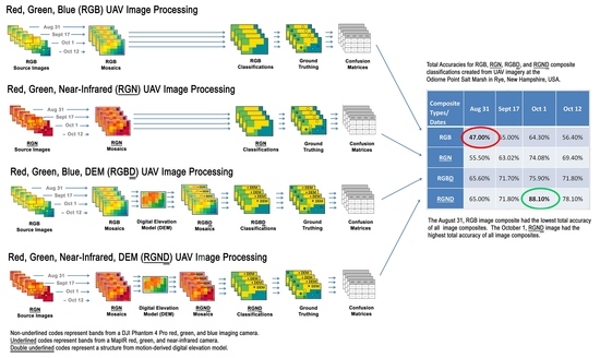
The objectives of our work were the following: First, both Red, Green, Blue (RGB) camera and Red, Green, Near-Infrared (RGN) camera salt marsh image classifications would be created and assessed to determine how their accuracies differed. Second, salt marsh image composites with and without an additional elevation layer would be created and assessed to determine if the new layer altered the accuracies of the classifications. Third, all these classifications would be created and their accuracy assessed over a time series of unique dates during late summer and early fall to determine how they differed seasonally from each other.

Thus, based on the findings of previous research literature, our project goal, and the intended objectives of this study, we hypothesized that:

• Using UAV imagery inclusive of a near-infrared band would improve vegetation classification total accuracies over those of true-color imagery alone within our study areas;
• Adding a DEM layer to UAV-derived imagery band combinations over our study areas would improve the imagery’s classification total accuracies;
• UAV-derived vegetation classification total accuracies would vary during the late summer and early fall within our study areas.

2. Materials and Methods

2.1. Study Areas

This work was conducted within a coastal salt marsh near the Odiorne Point State Park in Rye, New Hampshire, USA. Two study areas within this marsh were chosen to help to verify and compare the results between two separate locations. Study area 1 is a 1.9 hectare (4.7 acre) site with a vertical elevation range of 1.2 m (3.9 ft) located at 70°43′0.47″W by 43°2′25.93″N. The study area is flanked on the northeast and southwest by additional marsh habitat, on the northwest by mixed forests, and on the southeast by a large natural pool that separates most of the study area from the New Hampshire Route 1a state highway. This pool is regularly inundated by tidal flooding and is approximately one meter above the NAV88 tidal datum. It is hydrologically connected via a tidal creek to the southwest that extends approximately 1 km from its mouth, where it intersects the Piscataqua River. Other non-contiguous, smaller pools and pannes are also scattered across the landscape (Figure 1). Study area #2 is a 2.1 hectare (5.2 acre) site with a vertical elevation range of 1.45 m (4.8 ft) located at 70°43′31″W by 43°2′55″N. This study area directly abuts the New Hampshire Route 1a state highway to the north and west, where the road has been raised to meet a bridge crossing. The study area is also flanked to the east by an outcrop of mixed forest and other marsh habitat and to the south by the mouth of the creek that feeds the marsh. Other non-contiguous, smaller pools and pannes are also scattered across the landscape (Figure 1). Relative to study areas 1 and 2, the closest water level NOAA gauging station is at Fort Point, NH. This gauging station is approximately 5 km (3.1 mi) from study area 1 and 4 km (2.48 mi) from study area 2. The Fort Point gauging station reports a mean high water (MHW) level of 1.3 m (4.27 ft) and a mean tidal range of 2.63 m (8.62 ft) [81].

Within these study areas, low-marsh areas are dominated by smooth cordgrass (Spartina alterniflora), and high-marsh areas are dominated by a mix of salt hay (Spartina patens), spike grass (Distichlis spicata), blackgrass (Juncus gerardii), and the short form of smooth cordgrass (Spartina alterniflora short form) (

Table 1. Table of assessed plant species and abbreviations.

Plant Species	Abbreviations
Distichlis spicata	DiSp
Juncus gerardii	JuGe
Salicornia europaea (A.K.A. Salicornia depressa)	SaEu
Spartina alterniflora (tall form)	SpAl
Spartina alterniflora (short form)	SpAl-SF
Spartina patens	SpPa
Solidago sempervirens	SoSv

). In addition, two less-prevalent forb species, common glasswort (Salicornia europaea, A.K.A. Salicornia depressa) and seaside goldenrod (Solidago sempervirens), also occur within the study areas (Table 1). These seven species will be assessed within this research and will be referred heretofore by their lettered abbreviation codes, as listed in Table 1.

2.2. Methods and Materials

2.2.1. Spectral Assessment

In 2017 and 2018, multiple vegetation samples of the seven vegetation species assessed within this study were collected at a set of dispersed representative species patch locations across the marsh and then analyzed using an ASD Fieldspec 4 Hi-Res high-resolution spectroradiometer (Boulder, CO, USA) [82]. The spectroradiometer was optimized and calibrated to a standard white ceramic plate in a controlled laboratory environment under full-spectrum light conditions. Dense vegetation samples were split in half, laid crosswise over each other, and scanned with the spectroradiometer ten times each from four sides and then averaged to construct a spectral signature to smooth inconsistencies brought on by shadows and texture. This analysis was completed every two weeks to create a series of spectral vegetation data signature curves over the growing season. Reflectance measurements were calculated using the ASD to capture reflectance values from 350 µm to 2500 µm [82]. The curves were then assessed visually to review if and how the spectral characteristics of the vegetation species varied.

2.2.2. UAV Assessment

Approximately 200 UAV-derived high-resolution camera images were first captured over study areas 1 and 2 on 13 April 2018 and 1 May 2022, respectively, before any new seasonal growth occurred and when each year’s previous aboveground biomass was still matted down from the effects of the previous winter’s snowpack. Early spring was chosen for these flights to capture images that best represented bare earth elevation conditions [83,84,85,86]. The flights used a DJI Phantom 4 Pro UAV (Shenzhen, China) [87], equipped with a DJI, 20 MP normal true-color, 84° field-of-view (FOV) Red, Green, and Blue (R, G, B) camera (

Table 2. Specifications for the Phantom 4 Pro and MapIR Survey3 cameras.

Camera Specifications	Phantom 4 Pro Camera	MapIR Survey3 Camera
Sensor	1″ CMOS	Sony Exmor R IMX117
Resolution	20 MP	12 MP
Field of View	FOV 84°	FOV 87°
	Blue	Green (Centered at 550 nm)
Spectral Bands	Green	Red (Centered at 650 nm)
	Red	NIR (Centered at 850 nm)

), flying at an altitude of approximately 60 m (200 ft) and with front and side overlaps of approximately 80%. Image acquisition times on-site were limited to approximately one hour per study area per date, and images were acquired under low-tide conditions and within two hours of solar noon. The captured images were processed using Structure-from-Motion (SfM) photogrammetry techniques within Agisoft photogrammetric software, version 1.6 [88] to create a digital elevation model (DEM) for both study areas. The resulting models were then rectified to ground control points of fixed landmarks around the marsh using ArcGIS Pro software, version 2.6 [89]. Fixed landmarks included the bottom of fence posts and signposts, as well as manually placed wood stakes around the study areas. At the time of image collection, one-meter-diameter X-shaped ground targets were centered at the location of the fixed landmarks. Any surrounding vegetation was regularly cleared-back at each ground control point to allow for the acquisition of the target at ground level. All the ground control locations were chosen or placed at approximately the corners, perimeters, and centers of each study area to best aid in image rectification.

In study areas 1 and 2, sixty-four and fifty randomly sampled elevation points were collected, respectively, with a Trimble TSC3 data logger and a high-resolution, sub-centimeter vertical- and horizontal-accuracy Trimble R10 RTK GPS receiver (Westminster, CO, USA) [90]. A two-meter measuring pole equipped with a flat foot was also used for the RTK point collection to compensate for the varying spongy nature of the different marsh substrates across the study area. Accuracy checkpoints were distributed within all the vegetation classes across the whole marsh. Next, the UAV-derived DEM of study area 1 was shifted vertically to match the datum of the collected RTK points, resulting in a 4.60 cm (1.81 in) root-mean-square (RMS) accuracy for the model. In study area 2, the vertical datum shift resulted in a 10.68 cm (4.2 in) RMS accuracy between the spatially coincident points of the DEM and the sub-centimeter-accuracy RTK dataset.

In subsequent months after the spring images were acquired, approximately 200 additional UAV-derived high-resolution camera images were captured over each study area periodically during the late summer and early fall seasons (31 August, 17 September, 1 October, and 12 October 2018 for study area 1 and 14 September, 30 September, and 14 October for study area 2). These times of the year were chosen for UAV data collection because the ASD spectrometer assessments of 2017 and 2018 vegetation samples collected by us from June through October showed late summer and early fall to exhibit the largest spectral differences between vegetation species. Individual flight dates were prioritized based on an approximate two-week cycle, low-tide conditions, and local weather appropriate for staying within the operating parameters of the UAV. Note that only three flight dates were booked for study area 2 as opposed to four flights within study area 1 because of poor weather conditions and technical difficulties with the UAV when on site in late-August 2022. All the flights also carried a co-mounted MapIR, Survey3, 12 MP false-color, 87° FOV camera (San Diego, CA, USA) on the UAV [91] (Table 2). This camera is designed for vegetation mapping and captures spectral information in Red, Green, and Near Infrared (R, G, N) parts of the electromagnetic spectrum centered at 660 nm, 550 nm, and 850 nm, respectively. The images taken with this camera required an additional radiometric calibration using a calibration target with a known albedo and post-processing completed with MapIR Camera Control software, version 20221111. Heretofore, these spectral bands (layers) and the digital elevation model layer will be called “bands” and referred to by their single-letter codes, as listed in this and the previous paragraph. The DJI-derived band codes will not be underlined, the MapIR band codes will be underlined, and the digital elevation layer will be doubly underlined to distinguish them from each other (

Table 3. Project band composites and abbreviations. Composite band codes: R = red; G = green; B = blue; N = near infrared; D = digital elevation model. Non-underlined codes represent bands from a DJI Phantom 4 Pro red, green, and blue imaging camera. Underlined codes represent bands from a MapIR red, green, and near-infrared camera. Doubly underlined codes represent a structure from motion-derived digital elevation model.

Band Composite	Abbreviation
Red, Green, Blue	RGB
Red, Green, Blue, DEM	RGBD
Red, Green, Near Infrared	RGN
Red, Green, Near Infrared, DEM	RGND

). Because this work used multi-date imagery, the capture of imagery was always completed within about two hours of solar noon to maintain as much consistency as possible with regard to lighting and shadow conditions between the dates. The images were captured with approximately 80% front and side overlaps with an effective 1.67 cm ground resolution for the DJI true-color camera and at an effective 2.61 cm ground resolution for the MAPIR false-color camera. Flight planning and control was completed with Drone Deploy software, version 4.109.0.

All the collected RGB and RGN images were processed into collection-date-specific, common-spatial-resolution orthomosaics using Agisoft Metashape photogrammetry software [88] and a Universal Transverse Mercator Zone 19 projection. The mosaics were rectified to ground coordinates using ArcGIS Pro 2.6 software [89] and then clipped to a common study-area polygon. The pool, panne, and ditch water areas were masked out of the resulting mosaics so that only the vegetation areas would be assessed within this study. Additionally, the digital elevation models were clipped, masked, resampled, and rescaled to match their spectral mosaic counterparts’ spatial extents and spectral pixel value ranges. The rescaling of the elevation pixel value ranges was completed to match the overall upper and lower ranges of the spectral band values of each of the RGB and RGN composites, respectively, per study area. By completing the rescaling of the elevation pixel values this way, we provided a standardized elevation layer for a common analysis per composite type, per study area. Each RGB and RGN mosaic was then composited with their corresponding clipped digital elevation model D band to form RGBD and RGND composites for each sampling date for further assessment (Table 3).

Maximum likelihood supervised classifications were completed on each band composite using ArcGIS software, version 10.5.1 [92] for each study area. Study areas 1 and 2 used 196 and 60 training polygons, respectively, to delineate SpAl, SpAl-SF, SpPa, DiSp, JuGe, SaEu, and SoSv vegetation types. All the resulting classifications were then run through an eight-pixel neighborhood majority filter to reduce the speckling brought on by the effects of small shadows caused by inconsistent textures across the landscape.

Next, we completed an accuracy assessment on each of the resulting classifications. Within our study, over 2600 common stratified randomly sampled assessment points were created to assess the accuracy of our image classifications. A 50 point-per-class minimum was utilized where possible within this analysis based on Congalton’s (1991) [93] sampling rule of thumb. Ground truth classes were observed and recorded per point based on the air-truthing of the project’s high-resolution RGB imagery. In-person GPS-derived ground observation values collected during the 2018 and 2022 seasons and follow-up in-person verification of class patches were also used to inform further the air-truthing of the classifications.

Confusion matrices were created for each image band composite (RGB, RGN, RGBD, and RGND) and collection-date combination for the two study areas (31 August, 17 September, 1 October, and 12 October 2018 for study area 1 and 14 September, 30 September, and October 14 for study area 2. Confusion matrix tables [92] are used to compare and quantify the number of cross-class matches (Cross-Class Accuracy: CCA) and mismatches (Cross-Class Confusion: CCC) between the observed and classified data (

Table 4. Table of classification accuracy terms and abbreviations.

Term	Abbreviation
Cross Class Accuracy	CCA
Cross Class Confusion	CCC
Producer Accuracy	PA
User Accuracy	UA
Total Accuracy	TA

). The reproportioning of these quantities was then completed via a procedure called MARGFIT [94]. MARGFIT is an iterative fitting procedure that forces the sums of values from each row and column to equal 1, thus allowing for each cell value to be proportionally comparable to each other [92]. Within this work, we defined no confusion between class pairs to have a CCC of 0%, low confusion between classes to have a CCC of >0% but ≤10%, medium confusion between class pairs to have CCC of >10% but ≤20%, and high confusion between class pairs to have CCC of >20%.

Individual class and full-matrix accuracies were assessed through the calculation of user accuracies (UAs), producer accuracies (PAs), and total accuracies (TAs) (Table 4). UAs are calculated from the percentage of matches relative to all the observations within a class from a user’s perspective. PAs are calculated from the percentages of matches relative to all the observations within a class from the producer’s perspective. TAs are calculated from the percentage of all the matches relative to all the observations within the matrix. A Kappa statistic, KHAT, was also calculated as a measure of the total correspondence between observed and classified data, but this statistic does not assume independence between the classes, as does the TA measure [92,95]. Furthermore, all the classifications were tested and confirmed to be significantly different from each other using a test statistic that considers the Kappa and variance of Kappa statistics for each matrix [92].

Lastly, a salt marsh elevation profile was created for the vegetation base (ground-level) elevations at each study area (1 and 2). This was completed by calculating the zonal mean and standard deviation statistics on each digital-elevation-model layer per vegetation zone of the classification with the best TA. The results were ordered by mean elevation and vegetation class. Finally, non-parametric Welch post hoc pairwise comparison and Games–Howell test values were calculated for 350 stratified random samples (50 per class) to check the statistical difference between the base elevations for each possible pair of vegetation types. These tests were utilized because the data did not meet the equal variances assumption of an ANOVA test.

3. Results

3.1. Spectral Analysis

Visual inspection of the ASD spectroradiometer reflectance curves created over the growing season for each vegetation species assessed within this study showed that each species reached its peak distinction (separation from other curves) at different times from each other. For instance, Juncus gerardii (JuGe) begins to show strong spectral distinctions from all the other vegetation types by mid-August, with significantly less reflectance than the other species in the visual and NIR parts of the spectrum (Figure 2a). Other species’ spectral curves show that their times of most spectral distinction occur in late summer and early fall. Notably, the SpAl and SpAl-SF spectra separate from each other more in the visual and NIR parts of the spectrum for the 1 October samples than for the 14 September samples (Figure 2b). However, SpPa and DiSp separate from each other in both the visual and NIR parts of the spectrum for both the 14 September and the 1 October samples (Figure 2b,c). The SaEu curve, though spectrally distinct within the NIR part of the spectrum in August (Figure 2a), becomes spectrally distinct in both the visible and NIR parts of the spectrum for the 1 October samples (Figure 2c). The SoSv sample, though spectrally distinct within both the visual and NIR parts of the spectrum in the 14 September curve (Figure 2b), loses its distinction in the visual part of the spectrum by 1 October (Figure 2c). Also, although not specific to the spectral ranges of the cameras carried on the UAV within this study, SpAl vs. SpAl-SF, SpPa vs. DiSp, and JuGe also show strong distinctions in dryness to each other in the 1 October curve’s water absorption bands centered around 1450 and 1950 nm (Figure 2c). SoSv, however, shows the most distinction within this range of the curve for the 14 September samples (Figure 2b), but SaEu remains succulent, with low water-absorption band values through the whole of the season (Figure 2a–c). An unexplained anomaly also occurs between 1800 and 1900 nm in the 1 October curves (Figure 2c), showing a peak in this reflectance range that does not occur at any other time of the season.

3.2. UAV Analysis for Study Area 1

This research examined how band composites (RGB, RGN, RGBD, and RGND) and collection dates (31 August, 17 September, 1 October, and 12 October) affected classification accuracies within the project’s study area 1. Completing this analysis included the creation of sixteen statistically different (α = 0.05) maximum likelihood image classifications for each composite per collection date (Figure 3a–d) and sixteen corresponding MARGFIT confusion matrices (

Table A1. (a) Study Area 1—31 August 2018—RGB composite MARGFIT normalized confusion matrix. (b) Study Area 1—17 September 2018—RGB composite MARGFIT normalized confusion matrix. (c) Study Area 1—1 October 2018—RGB composite MARGFIT normalized confusion matrix. (d) Study Area 1—12 October 2018—RGB composite MARGFIT normalized confusion matrix.

(a)
Class	JuGe	SpPa	SaEu	SpAl	SoSv	DiSp	SpAl-SF	UA	Kappa C
JuGe	50.1%	2.0%	20.8%	6.7%	0.5%	11.7%	8.1%	52.9%
SpPa	0.8%	46.2%	3.1%	12.7%	16.6%	15.3%	5.4%	54.8%
SaEu	27.7%	0.9%	59.3%	4.8%	1.1%	3.9%	2.6%	37.3%
SpAl	8.1%	6.3%	13.2%	29.8%	7.8%	6.4%	28.5%	35.6%
SoSv	0.7%	28.8%	1.6%	10.6%	41.2%	14.4%	2.6%	16.4%
DiSp	8.3%	10.9%	0.8%	8.8%	21.7%	37.2%	12.3%	55.8%
SpAl-SF	4.5%	5.0%	1.2%	26.7%	11.1%	11.0%	40.6%	33.0%
PA	64.8%	53.5%	7.0%	51.5%	2.3%	54.0%	24.8%	47.0%
Kappa C.									0.3423
(b)
Class	JuGe	SpPa	SaEu	SpAl	SoSv	DiSp	SpAl-SF	UA	Kappa C
JuGe	69.4%	1.9%	10.6%	3.6%	1.0%	9.6%	4.0%	63.8%
SpPa	1.1%	60.9%	1.4%	9.1%	9.2%	14.5%	3.8%	57.5%
SaEu	9.3%	1.7%	82.0%	1.5%	2.7%	1.1%	1.8%	81.4%
SpAl	8.6%	6.9%	3.7%	38.2%	5.2%	9.6%	27.9%	40.7%
SoSv	0.9%	2.2%	1.5%	12.3%	73.7%	4.7%	4.8%	67.6%
DiSp	9.7%	17.4%	0.3%	11.5%	2.4%	51.1%	7.6%	61.6%
SpAl-SF	1.1%	9.0%	0.6%	23.8%	5.8%	9.4%	50.2%	46.4%
PA	73.9%	58.6%	31.5%	55.5%	25.0%	60.9%	33.0%	55.0%
Kappa C.									0.4419
(c)
Class	JuGe	SpPa	SaEu	SpAl	SoSv	DiSp	SpAl-SF	UA	Kappa C
JuGe	70.4%	3.3%	3.3%	3.1%	4.3%	7.3%	8.4%	63.0%
SpPa	3.1%	67.0%	1.0%	3.4%	3.0%	19.2%	3.5%	66.2%
SaEu	3.2%	0.7%	91.9%	0.1%	0.5%	0.8%	3.0%	93.8%
SpAl	9.6%	2.7%	2.7%	35.0%	24.6%	2.5%	22.9%	59.5%
SoSv	1.3%	8.8%	1.0%	47.4%	28.3%	9.8%	3.6%	6.6%
DiSp	8.8%	16.3%	0.1%	1.6%	11.6%	57.1%	4.5%	69.8%
SpAl-SF	3.7%	1.3%	0.2%	9.4%	27.8%	3.5%	54.2%	55.6%
PA	74.1%	59.3%	64.6%	67.4%	0.8%	74.2%	54.7%	64.3%
Kappa C									0.5572
(d)
Class	JuGe	SpPa	SaEu	SpAl	SoSv	DiSp	SpAl-SF	UA	Kappa C
JuGe	62.5%	5.2%	7.1%	6.8%	1.5%	9.1%	7.9%	53.5%
SpPa	5.8%	65.8%	2.3%	3.1%	0.1%	17.8%	5.0%	62.0%
SaEu	4.5%	2.8%	79.3%	3.9%	0.4%	1.5%	7.7%	74.8%
SpAl	7.8%	4.4%	9.4%	41.2%	5.9%	2.9%	28.5%	50.1%
SoSv	0.8%	1.8%	0.8%	20.6%	62.3%	9.1%	4.6%	48.6%
DiSp	13.1%	18.1%	0.4%	5.0%	3.7%	54.5%	5.2%	66.4%
SpAl-SF	5.5%	2.1%	0.8%	19.4%	26.1%	5.1%	41.1%	40.1%
PA	68.7%	58.7%	24.8%	59.6%	7.0%	68.2%	35.8%	56.4%
Kappa C									0.4585

a–d,

Table A2. (a) Study Area 1—31 August 2018—RGN composite MARGFIT normalized confusion matrix. (b) Study Area 1—17 September 2018—RGN composite MARGFIT normalized confusion matrix. (c) Study Area 1—1 October 2018—RGN composite MARGFIT normalized confusion matrix. (d) Study Area 1—12 October 2018—RGN composite MARGFIT normalized confusion matrix.

(a)
Class	JuGe	SpPa	SaEu	SpAl	SoSv	DiSp	SpAl-SF	UA	Kappa C
JuGe	59.6%	0.3%	23.1%	0.5%	0.5%	6.7%	9.4%	67.1%
SpPa	0.5%	56.5%	1.4%	7.9%	1.0%	27.4%	5.3%	54.0%
SaEu	6.2%	7.6%	3.8%	12.2%	64.0%	4.2%	1.8%	0.0%
SpAl	4.0%	4.9%	1.9%	62.7%	0.1%	8.3%	18.2%	63.0%
SoSv	5.2%	9.0%	42.0%	1.8%	27.6%	8.2%	6.2%	47.9%
DiSp	15.6%	17.9%	4.7%	6.8%	5.7%	40.3%	9.0%	55.2%
SpAl-SF	8.9%	3.8%	23.1%	8.2%	1.2%	4.8%	50.1%	44.1%
PA	60.3%	52.7%	0.0%	73.6%	28.2%	49.6%	65.4%	55.5%
Kappa C									0.4522
(b)
Class	JuGe	SpPa	SaEu	SpAl	SoSv	DiSp	SpAl-SF	UA	Kappa C
JuGe	74.5%	0.2%	5.1%	0.7%	1.1%	10.9%	7.5%	75.8%
SpPa	0.4%	60.4%	0.5%	5.8%	9.0%	19.2%	4.8%	55.6%
SaEu	4.8%	1.3%	72.9%	9.9%	8.9%	1.8%	0.6%	77.3%
SpAl	4.0%	2.7%	0.1%	71.8%	0.7%	8.7%	12.1%	73.9%
SoSv	1.1%	12.2%	14.8%	0.9%	58.2%	4.8%	8.0%	40.0%
DiSp	10.6%	17.5%	1.3%	4.1%	12.8%	49.7%	4.0%	63.7%
SpAl-SF	4.6%	5.7%	5.5%	6.8%	9.5%	4.9%	63.1%	53.4%
PA	66.3%	66.1%	23.0%	75.5%	19.0%	57.5%	76.9%	63.2%
Kappa C.									0.5478
(c)
Class	JuGe	SpPa	SaEu	SpAl	SoSv	DiSp	SpAl-SF	UA	Kappa C
JuGe	83.1%	0.8%	3.2%	2.5%	1.4%	5.0%	4.0%	80.8%
SpPa	0.2%	78.0%	1.7%	1.3%	4.7%	12.9%	1.1%	75.8%
SaEu	1.1%	3.5%	86.7%	0.5%	2.5%	0.3%	5.5%	86.0%
SpAl	4.6%	0.6%	0.1%	73.4%	1.5%	2.6%	17.4%	80.6%
SoSv	2.0%	7.4%	6.3%	7.3%	50.8%	8.1%	18.1%	28.1%
DiSp	2.5%	9.1%	0.1%	4.5%	10.0%	70.6%	3.1%	77.1%
SpAl-SF	6.4%	0.7%	2.0%	10.5%	29.1%	0.5%	50.8%	60.4%
PA	85.7%	82.9%	70.7%	67.2%	12.8%	83.4%	65.9%	74.8%
Kappa C									0.6884
(d)
Class	JuGe	SpPa	SaEu	SpAl	SoSv	DiSp	SpAl-SF	UA	Kappa C
JuGe	78.2%	0.5%	8.0%	0.8%	2.1%	7.2%	3.4%	70.2%
SpPa	1.1%	72.3%	5.4%	0.3%	1.8%	14.2%	4.8%	77.0%
SaEu	1.2%	6.2%	69.6%	0.8%	0.6%	3.9%	17.8%	51.4%
SpAl	2.3%	0.3%	0.1%	79.0%	3.3%	2.7%	12.3%	85.7%
SoSv	0.6%	5.4%	0.7%	9.7%	55.4%	7.8%	20.5%	29.7%
DiSp	10.6%	14.0%	0.2%	4.8%	4.9%	61.8%	3.8%	68.5%
SpAl-SF	6.0%	1.4%	16.1%	4.7%	31.9%	2.4%	37.5%	52.2%
PA	81.9%	64.4%	16.0%	77.7%	6.8%	78.7%	65.6%	69.4%
Kappa C									0.6190

a–d,

Table A3. (a) Study Area 1—31 August 2018—RGBD composite MARGFIT normalized confusion matrix. (b) Study Area 1—17 September 2018—RGBD composite MARGFIT normalized confusion matrix. (c) Study Area 1—1 October 2018—RGBD composite MARGFIT normalized confusion matrix. (d) Study Area 1—12 October 2018—RGBD composite MARGFIT normalized confusion matrix.

(a)
Class	JuGe	SpPa	SaEu	SpAl	SoSv	DiSp	SpAl-SF	UA	Kappa C
JuGe	57.2%	2.2%	12.4%	0.2%	3.9%	14.7%	9.4%	57.5%
SpPa	1.4%	60.3%	4.2%	1.4%	7.9%	15.5%	9.5%	61.8%
SaEu	26.5%	2.6%	62.0%	1.7%	0.2%	5.6%	1.5%	39.8%
SpAl	0.3%	0.6%	6.6%	90.4%	0.0%	1.7%	0.3%	93.0%
SoSv	0.1%	8.0%	0.2%	0.1%	85.9%	2.3%	3.5%	79.5%
DiSp	9.3%	16.9%	2.1%	4.2%	1.5%	49.8%	16.3%	63.8%
SpAl-SF	5.4%	9.5%	12.5%	2.1%	0.5%	10.5%	59.6%	52.0%
PA	75.0%	57.7%	19.4%	92.1%	63.4%	54.7%	65.3%	65.6%
Kappa C									0.5785
(b)
Class	JuGe	SpPa	SaEu	SpAl	SoSv	DiSp	SpAl-SF	UA	Kappa C
JuGe	70.8%	1.4%	8.0%	0.0%	3.4%	10.4%	6.0%	66.7%
SpPa	1.2%	66.3%	3.2%	1.4%	4.9%	16.1%	7.0%	64.6%
SaEu	11.1%	1.6%	80.5%	1.1%	0.1%	3.5%	2.1%	67.5%
SpAl	0.1%	1.1%	3.1%	92.7%	0.1%	2.2%	0.6%	94.8%
SoSv	0.6%	4.0%	0.2%	0.1%	89.2%	2.5%	3.5%	84.5%
DiSp	11.5%	16.9%	1.3%	2.7%	2.0%	55.0%	10.6%	67.3%
SpAl-SF	4.7%	8.7%	3.7%	2.0%	0.4%	10.3%	70.2%	63.6%
PA	78.5%	63.6%	57.0%	91.9%	69.8%	62.3%	71.1%	71.7%
Kappa C									0.6528
(c)
Class	JuGe	SpPa	SaEu	SpAl	SoSv	DiSp	SpAl-SF	UA	Kappa C
JuGe	73.0%	3.0%	2.6%	0.1%	6.5%	7.4%	7.6%	67.0%
SpPa	3.6%	69.9%	0.8%	1.7%	1.5%	18.7%	3.7%	68.1%
SaEu	4.8%	0.3%	92.0%	0.1%	0.2%	0.8%	1.7%	92.5%
SpAl	2.4%	0.7%	2.8%	91.5%	0.1%	1.7%	0.7%	92.5%
SoSv	1.3%	4.5%	0.1%	0.1%	88.0%	2.3%	3.9%	79.7%
DiSp	8.0%	18.6%	0.4%	3.2%	2.0%	63.6%	4.1%	72.3%
SpAl-SF	6.8%	3.1%	1.2%	3.4%	1.8%	5.5%	78.3%	77.1%
PA	80.8%	61.8%	69.4%	91.7%	69.0%	72.8%	76.4%	75.9%
Kappa C									0.7030
(d)
Class	JuGe	SpPa	SaEu	SpAl	SoSv	DiSp	SpAl-SF	UA	Kappa C
JuGe	61.5%	5.2%	8.2%	0.1%	3.4%	11.3%	10.3%	56.7%
SpPa	6.0%	66.4%	3.3%	0.8%	0.3%	17.3%	5.9%	64.3%
SaEu	11.7%	1.4%	80.2%	0.8%	0.2%	1.8%	4.0%	71.1%
SpAl	1.0%	0.9%	4.1%	91.6%	0.1%	1.8%	0.6%	93.6%
SoSv	0.9%	2.4%	0.1%	0.1%	93.4%	1.9%	1.4%	87.8%
DiSp	12.2%	18.2%	0.7%	3.0%	2.2%	59.6%	4.2%	69.8%
SpAl-SF	6.8%	5.7%	3.4%	3.7%	0.5%	6.3%	73.6%	72.6%
PA	72.3%	60.2%	50.5%	91.9%	83.2%	67.5%	69.8%	71.8%
Kappa C									0.6536

a–d and

Table A4. (a) Study Area 1—31 August 2018—RGND composite MARGFIT normalized confusion matrix. (b) Study Area 1—17 September 2018—RGND composite normalized confusion matrix. (c) Study Area 1—1 October 2018—RGND composite MARGFIT normalized confusion matrix. (d) Study Area 1—12 October 2018—RGND composite MARGFIT normalized confusion matrix.

(a)
Class	JuGe	SpPa	SaEu	SpAl	SoSv	DiSp	SpAl-SF	UA	Kappa C
JuGe	61.9%	1.3%	7.0%	0.1%	6.0%	11.0%	12.8%	66.7%
SpPa	0.6%	63.0%	0.3%	0.7%	3.2%	26.0%	6.2%	57.2%
SaEu	15.2%	0.9%	72.1%	0.9%	0.9%	4.7%	5.3%	57.9%
SpAl	0.8%	0.9%	0.8%	93.6%	0.1%	2.6%	1.2%	93.0%
SoSv	1.5%	5.7%	0.1%	0.0%	86.0%	2.8%	3.9%	67.5%
DiSp	12.4%	21.2%	3.8%	2.6%	3.8%	45.4%	10.9%	60.7%
SpAl-SF	7.7%	7.0%	15.9%	2.0%	0.1%	7.5%	59.8%	50.0%
PA	62.9%	53.9%	14.0%	93.5%	83.1%	54.0%	74.2%	65.0%
Kappa C									0.5722
(b)
Class	JuGe	SpPa	SaEu	SpAl	SoSv	DiSp	SpAl-SF	UA	Kappa C
JuGe	74.1%	0.4%	3.8%	0.0%	3.6%	11.0%	7.0%	75.7%
SpPa	0.8%	65.2%	0.3%	1.3%	6.6%	21.0%	5.0%	61.4%
SaEu	6.1%	4.3%	84.6%	1.1%	0.4%	2.2%	1.3%	78.8%
SpAl	0.7%	0.7%	0.6%	93.4%	0.1%	2.5%	2.1%	93.9%
SoSv	1.1%	4.6%	0.1%	0.0%	86.1%	3.2%	5.0%	68.8%
DiSp	12.2%	18.0%	2.8%	2.9%	2.3%	54.3%	7.6%	66.1%
SpAl-SF	5.0%	7.0%	7.8%	1.3%	1.0%	5.9%	72.1%	64.4%
PA	69.6%	63.2%	48.6%	92.8%	81.4%	63.0%	78.3%	71.8%
Kappa C									0.6545
(c)
Class	JuGe	SpPa	SaEu	SpAl	SoSv	DiSp	SpAl-SF	UA	Kappa C
JuGe	85.2%	0.4%	3.2%	0.1%	2.5%	4.2%	4.5%	85.7%
SpPa	0.1%	86.4%	2.0%	0.2%	2.1%	8.4%	0.9%	85.2%
SaEu	2.5%	0.9%	94.4%	0.8%	0.2%	0.4%	1.0%	90.6%
SpAl	4.0%	0.4%	0.1%	94.2%	0.1%	0.4%	0.8%	95.2%
SoSv	1.8%	3.0%	0.1%	0.0%	92.0%	1.1%	2.2%	81.8%
DiSp	0.9%	7.4%	0.0%	3.2%	2.2%	83.8%	2.6%	86.0%
SpAl-SF	5.6%	1.6%	0.3%	1.6%	1.1%	1.8%	88.1%	91.6%
PA	89.1%	86.6%	86.9%	92.9%	86.2%	89.6%	80.6%	88.1%
Kappa C									0.8541
(d)
Class	JuGe	SpPa	SaEu	SpAl	SoSv	DiSp	SpAl-SF	UA	Kappa C
JuGe	75.1%	0.5%	6.1%	0.1%	3.0%	10.3%	5.0%	71.8%
SpPa	0.9%	76.4%	4.9%	0.1%	0.1%	12.4%	5.2%	77.5%
SaEu	8.1%	1.5%	82.3%	1.6%	0.1%	2.5%	3.9%	68.1%
SpAl	0.5%	0.7%	0.6%	94.3%	0.1%	1.7%	2.1%	96.1%
SoSv	1.5%	1.4%	0.1%	0.1%	92.2%	1.1%	3.7%	84.8%
DiSp	7.7%	16.7%	0.3%	2.8%	1.8%	66.4%	4.4%	71.1%
SpAl-SF	6.3%	2.8%	5.7%	1.0%	2.8%	5.7%	75.8%	80.2%
PA	81.1%	65.8%	68.7%	91.9%	84.1%	78.2%	71.6%	78.1%
Kappa C									0.7295

a–d).

The confusion matrices for the four RGB composite classifications yielded TAs ranging from 47.0% to 64.3% (

Table 5. (a) Table of confusion matrix Total Accuracies for RGB, RGN, RGBD, and RGND composite classifications created from UAV imagery acquired on 31 August, 17 September, 1 October, and 12 October 2018 at the Odiorne Point Salt Marsh in Rye, New Hampshire, USA. (Composite band codes: R = red; G = green; B = blue; N = near infrared; D = digital elevation model. Non-underlined codes represent bands from a DJI Phantom 4 Pro red, green, and blue imaging camera. Underlined codes represent bands from a MapIR red, green, and near-infrared camera. Doubly underlined codes represent a structure from motion-derived digital elevation model). (b) Table of confusion matrix Kappa coefficients for RGB, RGN, RGBD, and RGND composite classifications created from UAV imagery acquired on 31 August, 17 September, 1 October, and 12 October 2018 at the Odiorne Point Salt Marsh in Rye, New Hampshire, USA. (Composite band codes: R = red; G = green; B = blue; N = near infrared; D = digital elevation model. Non-underlined codes represent bands from a DJI Phantom 4 Pro red, green, and blue imaging camera. Underlined codes represent bands from a MapIR red, green, and near-infrared camera. Doubly underlined codes represent a structure from motion-derived digital elevation model).

(a)
Composites	Aug. 31	Sep. 17	Oct. 01	Oct. 12
RGB	47.00%	55.00%	64.30%	56.40%
RGN	55.50%	63.02%	74.08%	69.40%
RGBD	65.60%	71.70%	75.90%	71.80%
RGND	65.00%	71.80%	88.10%	78.10%
(b)
Composites	Aug. 31	Sep. 17	Oct. 01	Oct. 12
RGB	0.342	0.442	0.557	0.459
RGN	0.442	0.548	0.688	0.619
RGBD	0.579	0.653	0.703	0.654
RGND	0.572	0.655	0.854	0.723

a). The confusion matrices for the four RGN composite classifications revealed higher TAs than their four RGB composite classification counterparts, with percentages ranging from 55.5% to 74.2% (Table 5a). The confusion matrices for the four RGBD composite classifications revealed higher TAs than their four RGB composite classification counterparts, ranging from 65.6% to 75.9% (Table 5a), and the confusion matrices for the four RGND composite classifications revealed higher TAs than their four RGN composite classification counterparts, ranging from 65.0% to 88.1% (Table 5a).

CCCs varied across each composite type, although some trends were observable. The most frequent occurrence of high (>20%) CCC species pairs occurred within the RGB (Table A1a–d) and RGN (Table A2a–d) composites, and the least frequent occurrences of high (>20%) CCC species pairs occurred within the RGBD (Table A3a–d) and RGND (Table A4a–d) composites. The CCCs between SpPa and DiSp vs. JuGe and SpAl-SF were noticeably higher than those within the RGB and RGBD composites relative to their RGN and RGND counterparts, with a few exceptions, mostly within the 31 August composite. Also, the RGBD composite classifications had reduced CCCs between SpAl and SpAl-SF classes relative to their RGB counterparts (Table A3a–d).

UAs and PAs also varied across each composite type, although some notable findings were discovered. The confusion matrices for the four RGN composite classifications showed increased UAs and PAs in many classes (Table A2a–d) relative to their RGB counterparts. The confusion matrices for the four RGND composite classifications revealed improvements in UAs and PAs in most vegetation classes relative to their RGN counterparts, with notably large increases in UAs and PAs for SpAl and SoSv (Table A4a–d). Furthermore, the RGBD composites (Table A3a–d) showed improved UAs and PAs for SoSv relative to their RGB counterparts (Table A1a–d) but had less success at reducing CCCs between SpPa and DiSp, JuGe and DiSp, and JuGe and SpAl-SF.

A review of the confusion matrices by the acquisition date showed TAs ranging from 47.0% to 65.6% for the 31 August composite, 55.0% to 71.8% for the 17 September composites, 64.3% to 88.1% for the 1 October composite, and 56.4% to 78.1% for the 12 October composites (Table A1a–d, Table A2a–d, Table A3a–d and Table A4a–d). In general, the 31 August composite classifications created the lowest UAs and PAs, and the 1 October composite classifications created the highest, with some slight variations created by the 17 September and 12 October composite classifications (Table A1a–d, Table A2a–d, Table A3a–d and Table A4a–d). Overall, the 1 October classifications revealed the highest TAs, with the 1 October RGND composite classification having the highest TA of all the classifications, at 88.1% (Table 5a), and a Kappa coefficient of 0.854 (Table 5b).

Structure-from-motion (SfM) photogrammetry techniques allowed for the creation of a digital elevation model (base ground level elevations) for study area 1 (Figure 4a). The data were evaluated with Welch (α = 0.05) and Games–Howell post hoc pairwise comparison tests for vegetation-type pairs. The output of this test specifies different letters that indicate significant differences in the mean ground (base) elevations among the vegetation types. Quantitative analysis showed us that the base elevation values of SpAl (A) and SaEu (B) were significantly different (α = 0.05) from those of all the other vegetation classes but the base elevation values of SpAl-SF, SpPa, DiSp, and SoSv vegetation classes (C) and DiSp, JuGe, and SoSv (D) vegetation classes did not differ significantly from each other (Figure 5). A list of p-values for the vegetation-type pairs can be found in Appendix B 

Table A9. Post hoc pairwise comparison Games–Howell tests for vegetation-type pairs (α = 0.05) measuring statistical differences of vegetation types vs. elevations in study area 1.

Level	- Level	Difference	Std. Err. Dif.	DF	LCL	UCL	p-Value
SoSv	SpAl	0.367	0.032	52.792	0.215	0.519	<0.0001
JuGe	SpAl	0.285	0.009	97.978	0.245	0.325	<0.0001
DiSp	SpAl	0.258	0.011	90.140	0.209	0.307	<0.0001
SpPa	SpAl	0.244	0.009	97.680	0.205	0.284	<0.0001
SpAl-SF	SpAl	0.235	0.008	96.434	0.197	0.274	<0.0001
SoSv	SaEu	0.230	0.032	49.265	0.080	0.380	<0.0001
JuGe	SaEu	0.149	0.006	56.010	0.119	0.178	<0.0001
SaEu	SpAl	0.136	0.006	55.806	0.106	0.167	<0.0001
SoSv	SpAl-SF	0.131	0.032	51.937	−0.020	0.283	0.0772
SoSv	SpPa	0.122	0.032	52.383	−0.030	0.274	0.1237
DiSp	SaEu	0.123	0.009	52.716	0.081	0.162	<0.0001
SoSv	DiSp	0.109	0.033	55.946	−0.046	0.263	0.2436
SpPa	SaEu	0.108	0.006	56.623	0.080	0.137	<0.0001
SpAl-SF	SaEu	0.099	0.006	57.766	0.072	0.126	<0.0001
SoSv	JuGe	0.082	0.032	52.681	−0.071	0.234	0.5629
JuGe	SpAl-SF	0.050	0.009	96.770	0.0119	0.088	0.0009
JuGe	SpPa	0.041	0.009	97.825	0.001	0.080	0.0177
JuGe	DiSp	0.027	0.011	89.466	−0.021	0.075	0.5333
DiSp	SpAl-SF	0.023	0.010	84.050	−0.024	0.069	0.6829
DiSp	SpPa	0.014	0.010	87.487	−0.034	0.061	0.9659
SpPa	SpAl-SF	0.009	0.008	97.512	−0.029	0.046	0.9837

.

3.3. UAV Analysis of Study Area 2

This analysis examined how band composites (RGB, RGN, RGBD, and RGND) and collection dates (14 September, 30 September, and 14 October) affected the classification accuracies within the project’s study area 2. Completing this analysis included the creation of three statistically different (α = 0.05) maximum likelihood image classifications for each of the four composite collection dates (Figure 6a–d) and twelve corresponding MARGFIT confusion matrices (

Table A5. (a) Study Area 2—14 September, 2022—RGB composite MARGFIT normalized confusion matrix. (b) Study Area 2—30 September, 2022—RGB composite MARGFIT normalized confusion matrix. (c) Study Area 2—14 October 2022—RGB composite MARGFIT normalized confusion matrix.

(a)
Class	JuGe	SpPa	SaEu	SpAl	SoSv	DiSp	SpAl-SF	UA	Kappa C
JuGe	49.0%	5.3%	17.7%	0.4%	0.4%	13.9%	13.4%	50.4%
SpPa	8.8%	48.1%	0.3%	3.1%	8.2%	17.6%	14.0%	63.7%
SaEu	10.6%	5.3%	33.1%	9.1%	10.4%	26.0%	5.5%	0.0%
SpAl	3.2%	9.5%	1.4%	64.1%	0.5%	3.4%	17.8%	56.7%
SoSv	1.3%	18.1%	3.9%	1.1%	69.4%	3.1%	3.2%	63.6%
DiSp	10.6%	5.3%	33.1%	9.1%	10.4%	26.0%	5.5%	0.0%
SpAl-SF	16.6%	8.4%	10.4%	13.1%	0.8%	10.1%	40.7%	58.4%
PA	46.6%	70.8%	0.0%	33.5%	33.7%	0.0%	71.7%	59.0%
Kappa C									0.4140
(b)
Class	JuGe	SpPa	SaEu	SpAl	SoSv	DiSp	SpAl-SF	UA	Kappa C
JuGe	52.2%	9.9%	11.9%	2.9%	0.1%	9.7%	13.3%	48.2%
SpPa	8.2%	49.3%	0.1%	7.4%	2.1%	22.2%	10.7%	63.8%
SaEu	6.9%	0.8%	80.7%	1.7%	3.6%	2.7%	3.7%	78.3%
SpAl	0.8%	5.2%	1.3%	60.9%	16.2%	1.6%	14.1%	49.2%
SoSv	1.0%	16.5%	1.5%	1.2%	74.3%	1.9%	3.6%	71.7%
DiSp	16.8%	7.0%	3.8%	2.9%	2.1%	61.0%	6.4%	46.2%
SpAl-SF	14.2%	11.4%	0.7%	23.1%	1.5%	1.0%	48.2%	62.1%
PA	53.9%	67.2%	36.0%	13.0%	51.8%	6.1%	75.9%	60.3%
Kappa C									0.4360
(c)
Class	JuGe	SpPa	SaEu	SpAl	SoSv	DiSp	SpAl-SF	UA	Kappa C
JuGe	52.4%	21.3%	2.8%	5.3%	0.4%	1.4%	16.4%	38.9%
SpPa	12.4%	40.4%	0.3%	5.8%	1.4%	21.2%	18.5%	58.7%
SaEu	3.8%	1.7%	80.2%	2.0%	1.5%	2.0%	9.0%	55.6%
SpAl	3.5%	15.9%	1.5%	39.8%	27.7%	0.8%	10.8%	23.1%
SoSv	0.9%	5.0%	2.6%	20.9%	65.8%	1.4%	3.3%	66.7%
DiSp	8.1%	7.6%	2.7%	1.4%	1.0%	71.8%	7.4%	55.6%
SpAl-SF	18.9%	8.1%	9.8%	24.7%	2.3%	1.5%	34.7%	52.0%
PA	22.6%	54.0%	20.0%	10.0%	38.6%	25.5%	76.5%	51.9%
Kappa C									0.3000

a–c,

Table A6. (a) Study Area 2—14 September, 2022—RGN composite MARGFIT normalized confusion matrix. (b) Study Area 2—30 September, 2022—RGN composite MARGFIT normalized confusion matrix. (c) Study Area 2—14 October 2022—RGN composite MARGFIT normalized confusion matrix.

(a)
Class	JuGe	SpPa	SaEu	SpAl	SoSv	DiSp	SpAl-SF	UA	Kappa C
JuGe	60.8%	11.2%	2.6%	1.6%	0.8%	7.0%	16.0%	62.5%
SpPa	6.0%	47.9%	0.3%	5.3%	8.9%	20.8%	10.7%	62.7%
SaEu	7.0%	5.8%	35.5%	9.2%	10.9%	25.9%	5.7%	0.0%
SpAl	6.1%	4.8%	0.8%	69.4%	0.3%	6.7%	11.9%	65.6%
SoSv	3.5%	16.5%	5.9%	1.5%	67.3%	4.3%	1.0%	66.7%
DiSp	7.0%	5.8%	35.5%	9.2%	10.9%	25.9%	5.7%	0.0%
SpAl-SF	9.6%	8.0%	19.5%	3.7%	0.9%	9.3%	49.0%	67.7%
PA	46.7%	75.6%	0.0%	66.9%	21.7%	0.0%	76.9%	65.2%
Kappa C									0.5060
(b)
Class	JuGe	SpPa	SaEu	SpAl	SoSv	DiSp	SpAl-SF	UA	Kappa C
JuGe	66.0%	5.0%	0.2%	1.1%	0.2%	23.1%	4.5%	76.7%
SpPa	7.9%	52.8%	0.1%	4.1%	7.3%	17.4%	10.4%	65.3%
SaEu	1.6%	1.3%	86.7%	2.5%	1.9%	5.0%	1.2%	100.0%
SpAl	3.3%	3.8%	0.2%	84.7%	0.2%	2.0%	5.7%	77.5%
SoSv	1.3%	2.9%	2.2%	1.9%	87.0%	3.8%	0.9%	96.8%
DiSp	13.5%	18.9%	4.7%	4.2%	3.1%	41.4%	14.3%	18.2%
SpAl-SF	6.4%	15.3%	6.0%	1.6%	0.5%	7.3%	62.9%	71.5%
PA	63.3%	67.8%	30.0%	86.6%	36.6%	2.0%	84.4%	71.1%
Kappa C									0.5930
(c)
Class	JuGe	SpPa	SaEu	SpAl	SoSv	DiSp	SpAl-SF	UA	Kappa C
JuGe	60.0%	14.5%	0.9%	9.9%	0.6%	1.1%	13.0%	51.0%
SpPa	9.0%	43.3%	0.6%	1.3%	5.9%	27.2%	12.7%	63.6%
SaEu	7.0%	3.9%	46.2%	8.0%	11.1%	19.9%	4.1%	0.0%
SpAl	8.0%	4.6%	1.2%	68.6%	4.3%	0.5%	12.7%	59.8%
SoSv	0.5%	14.1%	3.3%	6.3%	72.4%	1.4%	2.0%	57.7%
DiSp	8.1%	10.5%	18.0%	3.1%	4.3%	38.7%	17.3%	18.2%
SpAl-SF	7.4%	9.2%	29.9%	2.9%	1.4%	11.1%	38.2%	64.9%
PA	59.4%	56.4%	0.0%	70.3%	54.9%	2.0%	72.9%	61.3%
Kappa C									0.4650

a–c,

Table A7. (a) Study Area 2—14 September, 2022—RGBD composite MARGFIT normalized confusion matrix. (b) Study Area 2—30 September, 2022—RGBD composite MARGFIT normalized confusion matrix. (d) Study Area 2—14 October 2022—RGBD composite MARGFIT normalized confusion matrix.

(a)
Class	JuGe	SpPa	SaEu	SpAl	SoSv	DiSp	SpAl-SF	UA	Kappa C
JuGe	52.0%	4.6%	30.2%	1.2%	0.6%	1.8%	9.7%	55.7%
SpPa	11.9%	54.0%	0.6%	4.4%	4.7%	8.1%	16.3%	67.4%
SaEu	10.2%	4.3%	46.7%	8.4%	10.1%	15.7%	4.6%	0.0%
SpAl	4.2%	4.2%	1.5%	77.1%	0.3%	0.5%	12.1%	69.9%
SoSv	0.7%	10.9%	3.1%	0.6%	83.5%	1.0%	0.3%	76.5%
DiSp	4.3%	13.3%	2.2%	0.4%	0.5%	66.7%	12.7%	40.5%
SpAl-SF	16.8%	8.8%	15.9%	7.9%	0.2%	6.2%	44.3%	64.1%
PA	52.9%	65.7%	0.0%	60.3%	74.7%	45.9%	71.2%	63.7%
Kappa C									0.4990
(b)
Class	JuGe	SpPa	SaEu	SpAl	SoSv	DiSp	SpAl-SF	UA	Kappa C
JuGe	65.5%	11.5%	4.2%	3.2%	0.4%	3.6%	11.5%	57.1%
SpPa	11.7%	55.1%	0.2%	5.4%	4.3%	10.0%	13.2%	67.4%
SaEu	1.6%	0.9%	92.8%	0.5%	1.5%	1.4%	1.4%	91.1%
SpAl	2.1%	4.0%	0.9%	78.0%	1.2%	1.1%	12.7%	72.9%
SoSv	1.6%	6.5%	0.5%	0.6%	89.9%	0.6%	0.4%	70.3%
DiSp	2.9%	9.9%	0.5%	0.2%	0.6%	80.6%	5.3%	50.7%
SpAl-SF	14.5%	12.1%	1.0%	12.1%	2.1%	2.7%	55.5%	67.3%
PA	55.0%	61.5%	82.0%	42.7%	85.5%	70.4%	75.9%	65.9%
Kappa C									0.5310
(c)
Class	JuGe	SpPa	SaEu	SpAl	SoSv	DiSp	SpAl-SF	UA	Kappa C
JuGe	54.8%	16.6%	0.8%	7.6%	7.0%	1.6%	11.6%	47.3%
SpPa	15.7%	48.8%	0.4%	4.2%	1.9%	10.9%	18.1%	62.6%
SaEu	3.5%	0.2%	89.7%	0.5%	1.0%	1.0%	4.3%	71.7%
SpAl	4.9%	6.1%	0.9%	74.5%	0.6%	0.6%	12.3%	62.3%
SoSv	1.3%	9.3%	0.9%	1.0%	86.6%	0.7%	0.2%	64.7%
DiSp	1.2%	7.5%	0.8%	0.3%	0.6%	83.1%	6.6%	55.9%
SpAl-SF	18.6%	11.5%	6.6%	12.0%	2.3%	2.1%	47.1%	60.5%
PA	32.9%	53.7%	66.0%	49.8%	79.5%	72.4%	74.2%	60.0%
Kappa C									0.4450

a–c and

Table A8. (a) Study Area 2—14 September, 2022—RGND composite normalized confusion matrix. (b) Study Area 2—30 September, 2022—RGND composite MARGFIT normalized confusion matrix. (c) Study Area 2—14 October 2022—RGND composite MARGFIT normalized confusion matrix.

(a)
Class	JuGe	SpPa	SaEu	SpAl	SoSv	DiSp	SpAl-SF	UA	Kappa C
JuGe	64.7%	11.9%	4.5%	1.4%	0.4%	3.3%	13.7%	64.2%
SpPa	7.2%	54.7%	0.6%	8.8%	7.6%	9.7%	11.4%	66.7%
SaEu	13.4%	1.5%	53.4%	3.4%	5.0%	5.6%	17.6%	10.0%
SpAl	3.6%	3.7%	1.2%	81.7%	0.3%	1.9%	7.5%	70.6%
SoSv	1.4%	8.9%	2.5%	0.5%	85.8%	0.8%	0.2%	73.2%
DiSp	1.9%	12.6%	2.5%	0.5%	0.7%	74.1%	7.8%	47.5%
SpAl-SF	7.9%	6.7%	35.3%	3.6%	0.1%	4.7%	41.8%	71.5%
PA	52.9%	71.5%	2.0%	72.4%	72.3%	48.0%	74.7%	68.0%
Kappa C									0.5590
(b)
Class	JuGe	SpPa	SaEu	SpAl	SoSv	DiSp	SpAl-SF	UA	Kappa C
JuGe	85.7%	3.1%	0.4%	1.9%	0.3%	3.8%	4.9%	87.2%
SpPa	4.8%	79.9%	0.3%	3.2%	3.2%	1.4%	7.4%	88.3%
SaEu	0.4%	0.3%	95.7%	0.8%	0.8%	0.9%	1.2%	97.7%
SpAl	2.2%	1.6%	0.3%	90.3%	0.2%	0.7%	4.8%	83.5%
SoSv	0.4%	3.1%	0.9%	0.7%	93.9%	0.7%	0.3%	92.0%
DiSp	1.5%	5.4%	0.7%	0.5%	0.5%	90.5%	0.8%	82.1%
SpAl-SF	5.1%	6.7%	1.8%	2.7%	1.1%	2.0%	80.6%	82.2%
PA	77.1%	79.8%	86.0%	89.1%	83.1%	79.6%	91.9%	85.1%
Kappa C									0.7960
(c)
Class	JuGe	SpPa	SaEu	SpAl	SoSv	DiSp	SpAl-SF	UA	Kappa C
JuGe	65.0%	11.6%	0.3%	8.4%	2.8%	0.3%	11.8%	52.8%
SpPa	14.0%	52.5%	0.3%	3.2%	4.9%	10.1%	15.1%	68.2%
SaEu	1.3%	0.6%	87.8%	1.7%	3.0%	2.5%	3.1%	89.5%
SpAl	5.4%	3.4%	0.3%	81.1%	0.4%	0.3%	9.0%	65.7%
SoSv	1.9%	8.6%	0.5%	0.4%	87.4%	0.5%	0.9%	62.8%
DiSp	2.1%	12.4%	0.8%	0.6%	1.0%	76.3%	6.9%	47.5%
SpAl-SF	10.5%	11.0%	10.0%	4.7%	0.5%	10.1%	53.2%	69.7%
PA	63.9%	54.6%	34.0%	77.8%	85.5%	48.0%	71.7%	65.0%
Kappa C									0.5280

a–c).

The confusion matrices for the three RGB composite classifications yielded TAs ranging from 51.9% to 60.3% (

Table 6. (a) Table of confusion matrix Total Accuracies for RGB, RGN, RGBD, and RGND composite classifications created from UAV imagery acquired over study area 2 on 14 September, 30 September, and 14 October 2022 at the Odiorne Point Salt Marsh in Rye, New Hampshire, USA. (Composite band codes: R = red; G = green; B = blue; N = near infrared; D = digital elevation model. Non-underlined codes represent bands from a DJI Phantom 4 Pro red, green, and blue imaging camera. Underlined codes represent bands from a MapIR red, green, and near-infrared camera. Doubly underlined codes represent a structure from a motion-derived digital elevation model.) (b) Table of confusion matrix Kappa coefficients for RGB, RGN, RGBD, and RGND composite classifications created from UAV imagery acquired over study area 2 on 14 September, 30 September, and 14 October 2022 at the Odiorne Point Salt Marsh in Rye, New Hampshire, USA. (Composite band codes: R = red; G = green; B = blue; N = near infrared; D = digital elevation model. Non-underlined codes represent bands from a DJI Phantom 4 Pro red, green, and blue imaging camera. Underlined codes represent bands from a MapIR red, green, and near-infrared camera. Doubly underlined codes represent a structure from motion-derived digital elevation model).

(a)
Composites	Sep. 14	Sep. 30	Oct. 14
RGB	59.0%	60.3%	51.9%
RGN	65.2%	71.1%	61.3%
RGBD	63.7%	65.9%	60.0%
RGND	68.0%	85.1%	65.0%
(b)
Composites	Sep. 14	Sep. 30	Oct. 14
RGB	0.41	0.44	0.30
RGN	0.51	0.59	0.47
RGBD	0.50	0.53	0.45
RGND	0.56	0.80	0.53

a). The confusion matrices for the three RGN composite classifications revealed higher TAs than those of their three RGB composite classification counterparts, with percentages ranging from 61.3% to 71.1% (Table 6a). The confusion matrices for the three RGBD composite classifications revealed higher TAs than those of their three RGB composite classification counterparts, ranging from 60.0% to 65.9% (Table 6a), and the confusion matrices for the three RGND composite classifications revealed higher TAs than those of their three RGN composite classification counterparts, ranging from 65.0% to 85.1% (Table 6a).

CCCs varied across each composite type, although some trends were observable. The most frequent occurrence of high (>20%)-CCC species pairs occurred within the RGB (Table A5a–c) and RGN (Table A6a–c) composites, and the least frequent occurrences of high (>20%)-CCC species pairs occurred within the RGBD (Table A7a–c) and RGND (Table A8a–c) composites. All the RGBD and RGND composite classifications had reduced CCCs between the SpAl vs. SpAl-SF classes and SpAl vs. SoSv classes relative to their RGB and RGN counterparts, with only a few exceptions within the 15 October composite. (Table A7a–c). All the RGN and RGND composite classifications had reduced CCCs between the JuGe and SpAl-SF classes relative to their RGB and RGBD counterparts, except within the 14 September image (Table A7a–c). Unlike in study area 1, in study area 2 the RGN and RGND composite classifications did not show a consistent reduction in CCCs between the SpPa and DiSp classes and their RGB and RGBD counterparts (Table A7a–c). UAs and PAs also varied across each composite type, although some notable findings were discovered. The RGN and RGND composite classifications showed increased UAs and PAs (Table A6a–c) relative to their RGB and RGN counterparts, with only a few exceptions occurring mostly within the SoSv and SaEu classes.

A review of the confusion matrices by the acquisition date showed TAs ranging from 59.0% to 68.0% for the 14 September composites, 60.3% to 85.1% for the 30 September composite, and 51.9% to 65.0% for the October 14 composites (Table A5a–c, Table A6a–c, Table A7a–c and Table A8a–c). In general, the 14 September and 14 October composite classifications created the lowest UAs and PAs, and the 30 September composite classifications created the highest (Table A5a–c, Table A6a–c, Table A7a–c and Table A8a–c). Overall, the 30 September classifications revealed the highest TAs, with the 30 September RGND composite classification having the highest TA of all the classifications, at 85.1% (Table 6a), and a Kappa coefficient of 0.80 (Table 6b).

Structure-from-motion (SfM) photogrammetry techniques allowed for the creation of a digital elevation model (base-level ground elevations) for study area 2 (Figure 7a). The data were evaluated with Welch (α = 0.05) and Games–Howell post hoc pairwise comparison tests for vegetation-type pairs. The output of this test specifies different letters that indicate significant differences in the mean ground (base) elevations among the vegetation types. Quantitative analysis showed us that the base elevation values of SpAl (A) were significantly different (α = 0.05) from those of all the other vegetation classes but the the base elevation values of SaEu and SoSv (B); SpAl-SF, DiSp, and JuGe (C); and SpAl-SF, SpPa, and JuGe (D) did not differ significantly from each other(Figure 8). A list of p-values for the vegetation-type pairs can be found in Appendix B,

Table A10. Post hoc pairwise comparison Games–Howell tests for vegetation-type pairs (α = 0.05) measuring statistical differences of vegetation types vs. elevations in study area 2.

Level	- Level	Difference	Std. Err. Dif.	DF	LCL	UCL	p-Value
SoSv	SpAl	0.390	0.016	62.378	0.316	0.464	<0.0001
SaEu	SpAl	0.360	0.014	49.080	0.292	0.428	<0.0001
DiSp	SpAl	0.258	0.015	50.521	0.190	0.327	<0.0001
JuGe	SpAl	0.224	0.020	97.970	0.131	0.317	<0.0001
SoSv	SpPa	0.223	0.013	61.927	0.160	0.286	<0.0001
SpAl-SF	SpAl	0.216	0.018	89.630	0.134	0.299	<0.0001
SaEu	SpPa	0.193	0.012	47.115	0.137	0.249	<0.0001
SoSv	SpAl-SF	0.174	0.012	63.487	0.116	0.231	<0.0001
SpPa	SpAl	0.167	0.019	93.256	0.081	0.253	<0.0001
SoSv	JuGe	0.166	0.016	62.597	0.093	0.239	<0.0001
SaEu	SpAl-SF	0.144	0.0105	49.152	0.094	0.193	<0.0001
SaEu	JuGe	0.136	0.014	49.084	0.069	0.203	<0.0001
SoSv	DiSp	0.132	0.007	17.398	0.097	0.167	<0.0001
SaEu	DiSp	0.102	0.002	54.195	0.093	0.111	<0.0001
DiSp	SpPa	0.091	0.012	49.155	0.034	0.148	<0.0001
JuGe	SpPa	0.057	0.018	93.755	−0.028	0.142	0.3098
SpAl-SF	SpPa	0.049	0.016	94.121	−0.024	0.122	0.3052
DiSp	SpAl-SF	0.042	0.011	51.859	−0.008	0.092	0.0999
DiSp	JuGe	0.034	0.014	50.575	−0.033	0.101	0.6319
SoSv	SaEu	0.030	0.006	15.125	−0.004	0.064	0.0586
JuGe	SpAl-SF	0.008	0.018	90.406	−0.073	0.089	0.9999

.

4. Discussion

4.1. Classification Total Accuracies

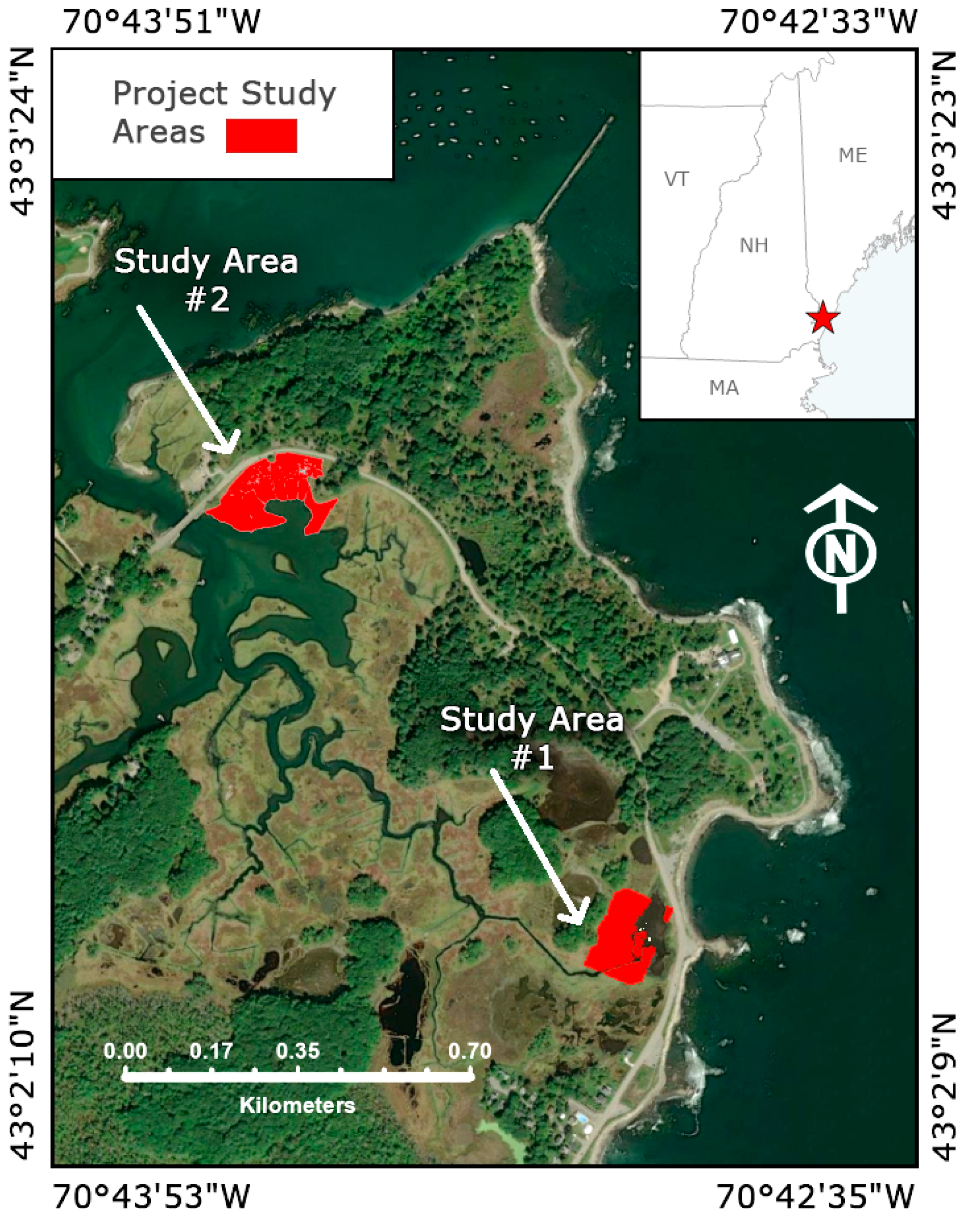
Within our research, we utilized a UAV to acquire aerial imagery for classifying and mapping the locations of plant species across a salt marsh environment. The use of <3 cm very high-spatial-resolution imagery enabled us to map the fine detail of narrow vegetation patch widths that are common within salt marshes. Our results showed that the 1 October RGND composite created from our UAV-derived imagery yielded the best total accuracy of 88.1% when classifying seven vegetation types across New Hampshire salt marsh study area 1 and 85.13% in study area 2.

4.1.1. Total Accuracies Relative to Other UAV Salt Marsh Vegetation Classification Studies

Of the identified studies where independent UAV imagery has been used for the classification of salt marsh plant species to date, our total accuracies do differ [67,71,72]. One study in Wadden Sea National Park, on Hallig Nordstrandischmoor Island, along the German coast of the North Sea [71], achieved between 92.9% and 95.0% accuracies. However, the Wadden Sea National Park study utilized object-based image analysis as opposed to pixel-based analysis, as was used within our study. The Wadden Sea National Park study also classified three vegetation and five non-vegetation classes, while our study classified seven vegetation classes. Although we did not compare object versus pixel-based analysis and various vegetation class granularities, we believe that this area of study could be fruitful within our study area. A second study that took place in the Cadiz Bay wetland in southern Spain achieved a 96% accuracy [72]. However, the Cadiz Bay wetland study used a hyperspectral camera to map four salt marsh species and one macroalga species within their study area vs. our seven vegetation species classes. Within a third study a multispectral camera and NDVI-derived layers were used for mapping the locations and seasonality of high and low salt marsh classes on Poplar Island in Maryland [67], USA. However, within the Nardin study, no confusion matrix classification accuracies were reported. Instead, the Nardin study correlated UAV-imagery-derived normalized-difference vegetation index (NDVI) measures with vegetation characteristics collected in the field [67].

4.1.2. Total Accuracies Relative to Other UAV Non-Salt Marsh Vegetation Classification Studies

Outside of salt marsh environments, UAVs have been shown to map species class granularities with total accuracies similar to those in our work. Lu and He (2017) [96] utilized UAV-acquired blue, green, and near-infrared (BGN) composite imagery to map species within temperate grasslands in Southern Ontario, Canada, to an approximately 85% accuracy using an object-based classification approach. Schiefer et al. (2020) [97] mapped forest tree species in the Southern Black Forest region of Germany with approximately 88% accuracy using UAV-acquired RGB imagery and neural networks. Neural networks rely on a training database that connects inputs to corresponding outputs that allow for the creation of complex functional relationships that are not easily envisioned by researchers [98]. Furthermore, other studies that utilized the sub-pixel analysis of lower-resolution hyperspectral imagery and hybrid-analysis-method techniques have been shown to have 85% and 93% TAs when classifying plant species at a class-level granularity [99,100]. These studies differ from our work in that they used various image processing techniques in place of a simple maximum likelihood classification technique to achieve similar classification accuracies at a species granularity level. Our technique, however, utilized the addition of near-infrared (NIR) layers, digital elevation model (DEM) layers, and classification date comparisons to achieve our highest total accuracies. We speculate that a hybrid approach for utilizing NIR and DEM layers and date comparisons in conjunction with either object-based, neural-network, or subpixel-analysis techniques could provide future methods that achieve higher classification accuracies of UAV imagery for mapping salt marsh species in New Hampshire.

4.1.3. Total Accuracies Relative to Other Non-UAV Wetland Vegetation Classification Studies

With regard to non-UAV imagery, the TAs of our research approximately align with the TAs of salt marsh and other wetland classification studies that utilized lower-spatial-resolution Landsat imagery [50,51,54]. However, in previous studies, the Landsat imagery that was used was only able to classify broad land-cover or vegetation classes [50,51,54]. For instance, Sun et al. (2018) [50] classified low-marsh, high-marsh, upper-high-marsh, and tidal-flat group classes using an NDVI time-series approach based on Landsat data within the Virginia Coast Reserve, USA, to achieve approximately 90% total accuracies. Harvey and Hill (2001) [54] classified three broad tropical wetland vegetation groups using unsupervised classifications of Landsat data for an area in northern Australia to achieve from 86% to 90% total accuracies. And, Wang et al. (2019) [51] classified eight broad land cover classes from Landsat data using random forest, support vector machine, and k-nearest neighbor machine learning algorithms for an estuary wetland in Lianyungang, China, to produce approximately 87%, 80%, and 77% total accuracies respectively. These uses of broad classifications of Landsat data speak to the findings of Belluco et al. (2006) [49] that emphasize the importance of higher-resolution imagery for the classification of salt marsh vegetation at the species granularity level. We believe that high-resolution UAV imagery, as used in our study in place of the lower-resolution Landsat imagery as utilized in previous salt marsh studies, allowed for similar classification accuracies to be achieved within our work but at a finer species class granularity in place of broad vegetation classes. The creation of these species class granularities can help to better contribute to a finer-scale understanding of where individual species live within salt marshes and how they are changing over time. The downside to the use of UAV imagery over Landsat imagery, however, is that UAV imagery has much smaller footprints relative to Landsat imagery, thus making the process for collecting UAV imagery a more time-consuming endeavor for large-area analysis.

4.2. A Finer Discussion of CCCs, UAs, and PAs

4.2.1. A Finer Discussion of RGB Composite Classifications

Although the total accuracies (TAs) between image classification types and dates can provide an overall assessment of which image classifications are best and worst to use to monitor salt marsh species, finer assessments of cross-class confusions (CCCs), user accuracies (UAs), and producer accuracies (PAs) can provide insights into the dynamics of why classification total accuracies differ from each other. The RGB composite classifications created for study area 1 and study area 2 displayed notable instances of where SpAl and SpAl-SF had relatively high CCC percentages (Table A1a–d and Table A5a–c). These high confusions might be explained by the fact that these two vegetation types are variants of the same species but are usually found in different parts of a salt marsh. SpAl usually resides within a wide tidal range in the low-marsh region below the mean high-tide line. 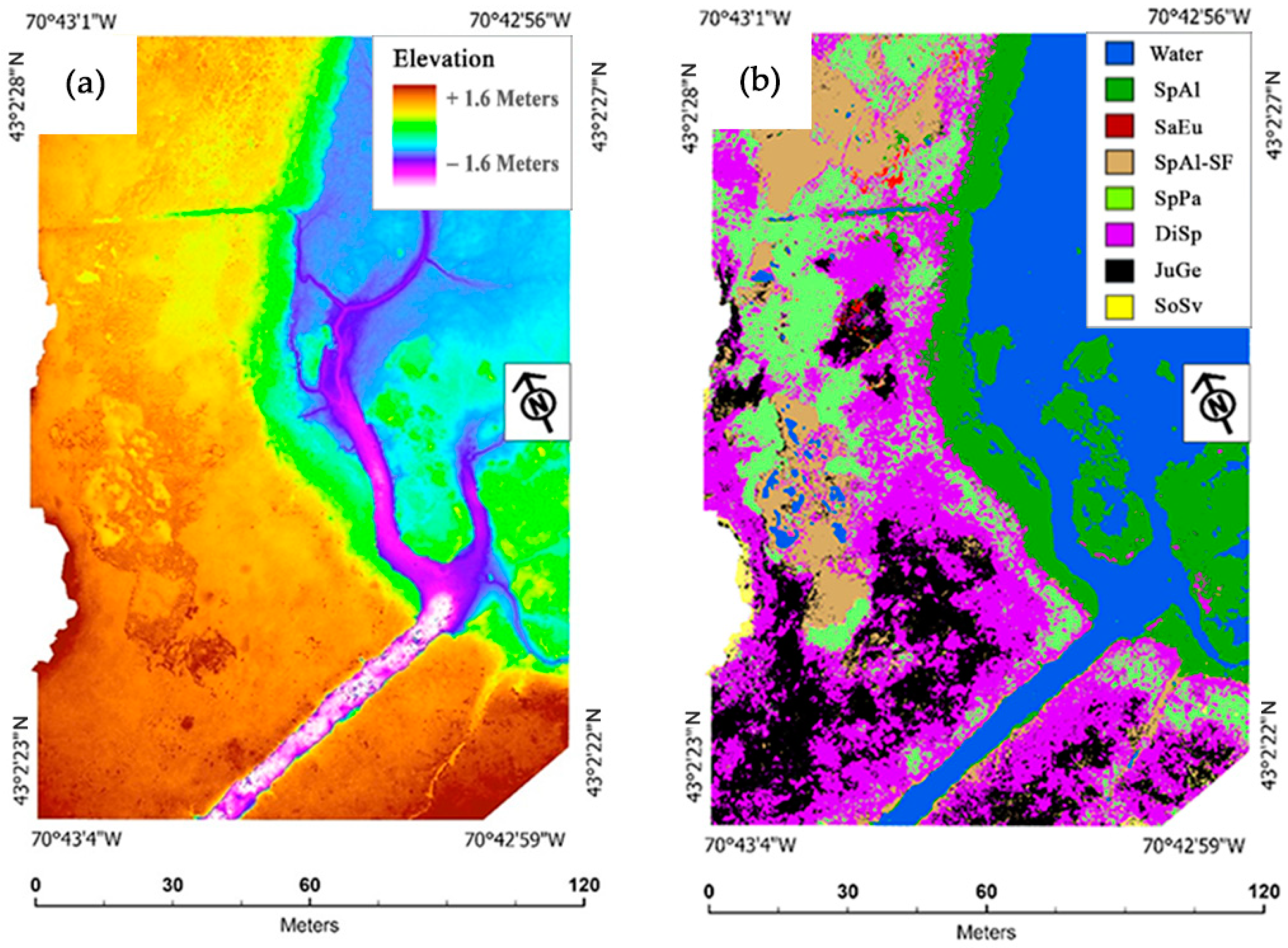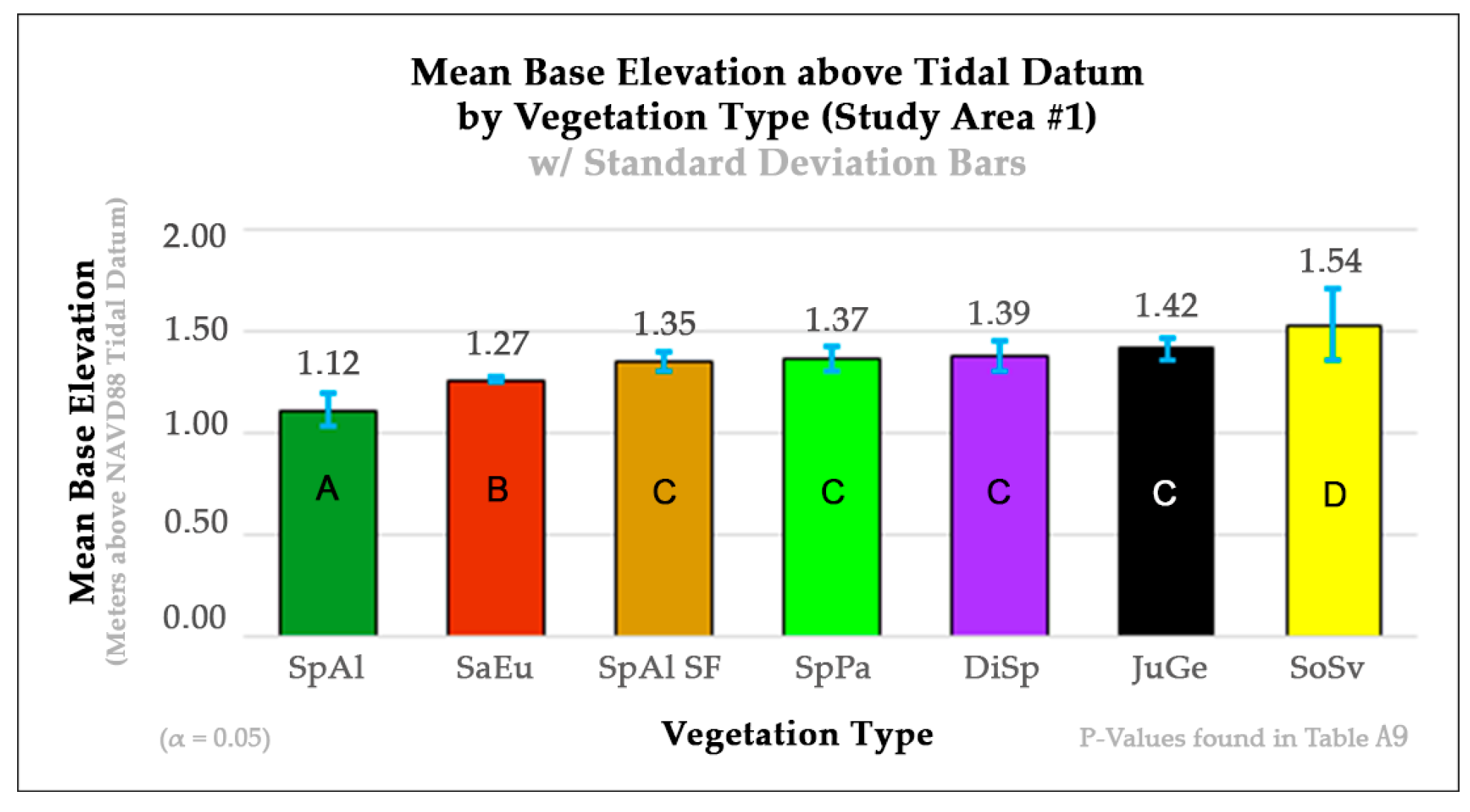Conversely, SpAl-SF resides within a shallow tidal range in low depressions across the high marsh [33]. The vegetation base elevation profiles created for each study area corroborate this explanation. 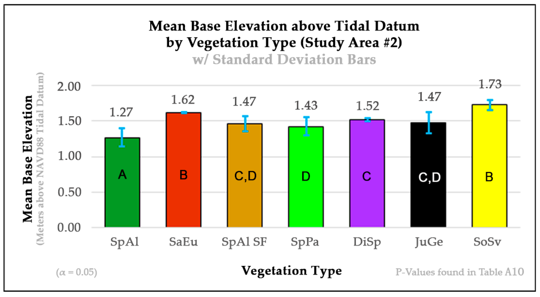In study area 1, SpAl had a mean base elevation of 1.12 m with a 0.076 m standard deviation, and SpAl-SF had a significantly different mean base elevation of 1.35 m with a 0.051 m standard deviation (Figure 5). 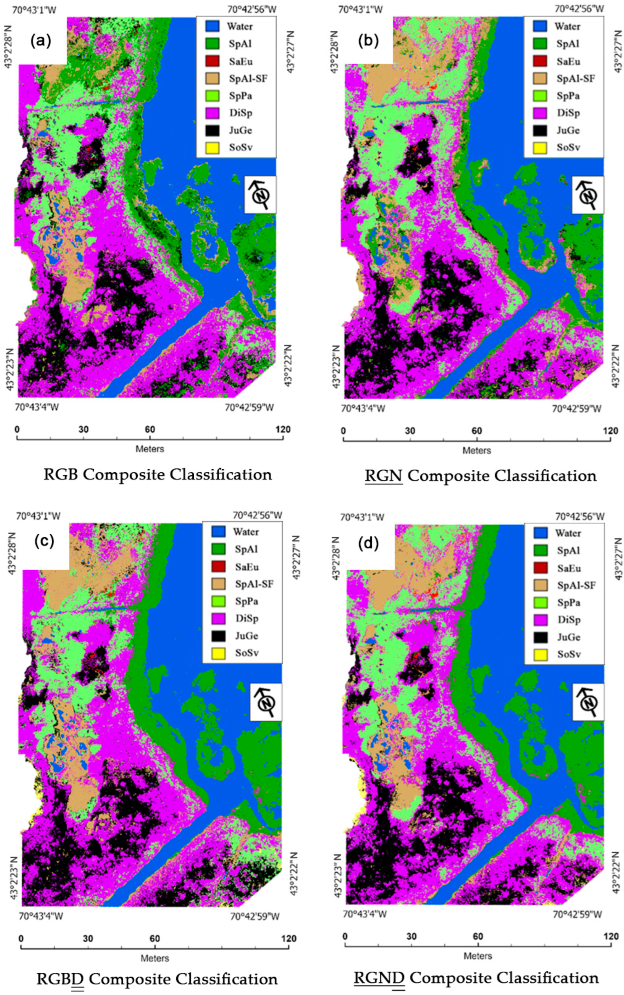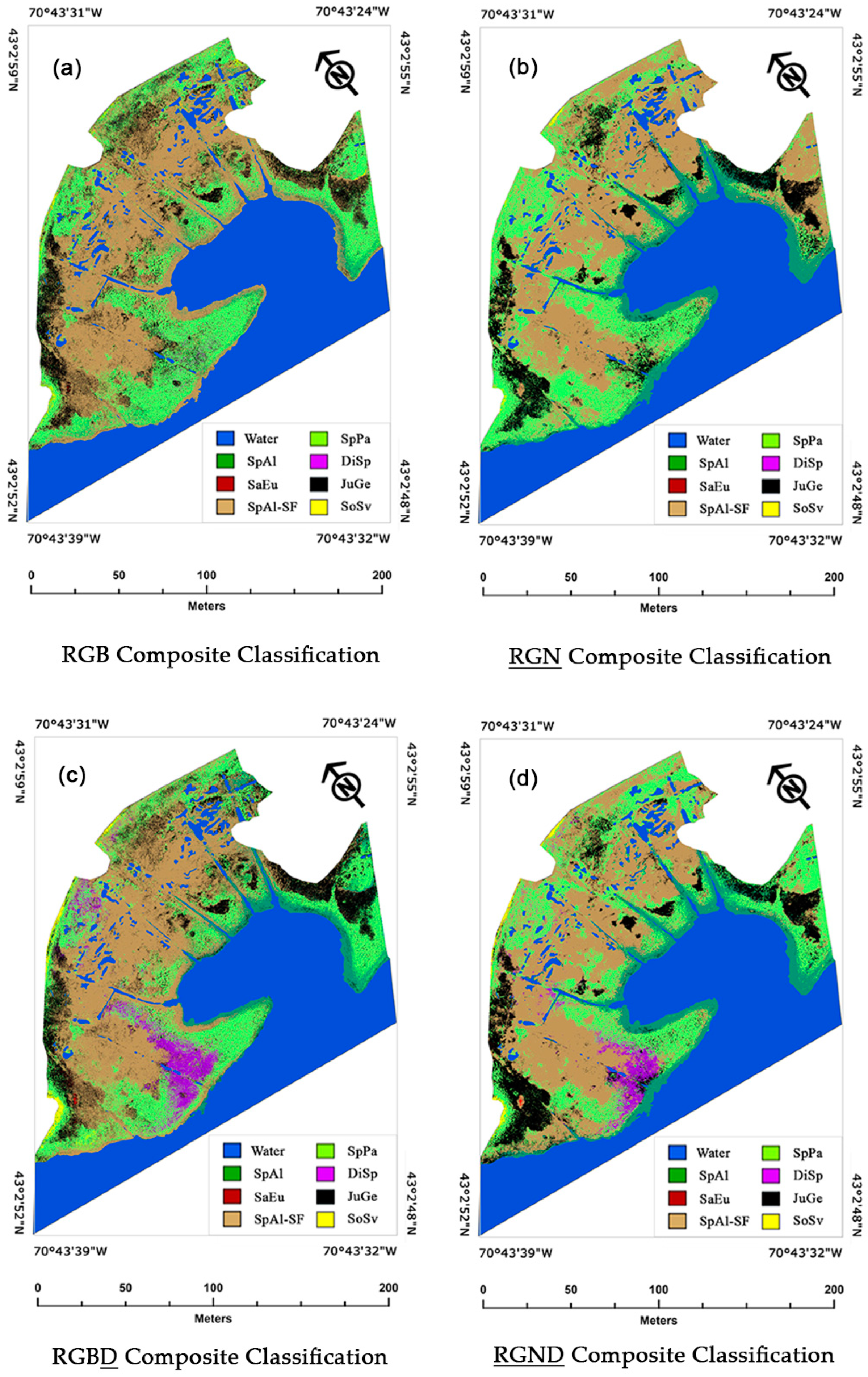In study area 2, SpAl had a mean base elevation of 1.27 m with a 0.13 m standard deviation, and SpAl-SF had a significantly different mean base elevation of 1.47 m with a 0.11 m standard deviation (Figure 8). In study area 1, the mapping of the 1 October RGB composite classification next to the 1 October RGND (the most accurate classification created for study area 1) provided a visual example of the large amounts of misclassified SpAl in the high marsh and misclassified SpAl-SF in the low marsh within the RGB classification (Figure 3a,d). Likewise, in study area 2, the mapping of the 30 September RGB composite classification next to the 30 September RGND (the most accurate classification created for study area 2) provided a visual example of the large amounts of misclassified SpAl-SF in the low marsh within the RGB classification (Figure 6a,d).

4.2.2. A Finer Discussion of RGN Composite Classifications

The RGN composite classifications created for study areas 1 and 2 yielded higher TAs than their RGB classification counterparts (Table 5a and Table 6a). This result was not unexpected because Artigas and Yang (2006) [77] showed how near-infrared segments of the electromagnetic spectrum in hyperspectral lab measurements could be useful to discriminate between prominent salt marsh species. In study area 1, the mapping of the 1 October RGB and RGN composite classifications next to the 1 October RGND (the most accurate classification created for study area 1) provided a visual example of how the RGN composite, inclusive of a near-infrared band, helped to reduce the number of misclassifications between classes, such as SpPa vs. DiSp and JuGe vs. SpAl-SF, in the high marsh relative to the RGB classification (Figure 3a,b,d). This example corresponds to a reduced CCC between the high-marsh classes, SpPa vs. DiSp and JuGe vs. SpAl-SF, within the RGN classification confusion matrices, relative to their RGB counterparts. In study area 2, the mapping of the 30 September RGB and RGN composite classifications next to the 30 September RGND (the most accurate classification created for study area 2) provided a similar visual example of how the RGN composite, inclusive of a near-infrared band, helped to reduce the number of misclassifications between classes, such as JuGe vs. SpPa and JuGe vs. SpAl-SF, in the high marsh relative to the RGB classification (Figure 6a,b,d). This example corresponds to a reduced CCC between the high-marsh classes, JuGe vs. SpPa and JuGe vs. SpAl-SF, within the 30 September and 14 October instances of the RGN classification confusion matrices, relative to their RGB counterparts. Within both study areas, the higher TAs, the visual improvements in high-marsh species accuracies, and the reduction in CCC between the high-marsh classes within the RGN composite classifications over their RGB counterparts support hypothesis 1 of this research, which states that using imagery inclusive of a near-infrared band can help to improve vegetation classification accuracies over true-color imagery alone.

This assertion of hypothesis 1 for salt marshes diverges from the findings of Lisein (2015) [101] and Grybas and Congalton (2021) [76] when they mapped tree species. Their work showed that true-color RGB camera imagery could be more effective when mapping tree species than multispectral imagery inclusive of a near-infrared band. However, these two studies differ from our study in that their work created single classifications with imagery from multiple dates, taking advantage of the changing phenology over time to classify tree species. Within our study, we have shown that imagery inclusive of a near-infrared band favored higher total accuracies than true-color imagery alone when mapping salt marsh species per individual date. We attribute the higher accuracies obtained with the MapIR RGN camera imagery over the accuracies obtained with the DJI RGB camera imagery because the former imagery tended to be more effective for classifying differences between the high-marsh species, SpPa vs. DiSp and JuGe vs. SpAl-SF, all of which comprised most of the vegetation cover across study area 1.

4.2.3. A Finer Discussion of RGBD Composite Classifications

The addition of an elevation layer, D, to the RGB composites in study areas 1 and 2 also yielded higher TAs than just their RGB composites alone (Table 5a and Table 6a). In both study areas, the creation of the RGBD composite classifications (Table A3a–d and Table A7a–c) revealed reduced CCC percentages between SpAl and SpAl-SF relative to their RGB counterparts (Table A1a–d and Table A5a–c). This reduction in CCC between these two spectrally similar classes is consistent with Lee and Shan’s (2003) [78] findings that the inclusion of a digital elevation data layer within coastal IKONOS imagery can help to increase the classification accuracies of classes with similar spectral characteristics.

In study area 1, the RGBD composites (Table A3a–d) also yielded improved UAs and PAs for SoSv relative to their RGB counterparts (Table A1a–d) but had less success at reducing CCCs between SpPa and DiSp, JuGe and DiSp, and JuGe and SpAl-SF. The addition of the digital elevation band, D, to an RGB composite did more to increase accuracies in the low-marsh and terrestrial-border species of SpAl and SoSv but was not as effective at increasing accuracies between high-marsh species, such as SpAl-SF, SpPa, DiSp, and JuGe. The assessment of the vegetation base elevation marsh profile for study area 1 reveals that this might be the case because SpAl-SF, SpPa, and JuGe all reside at similar vertical base elevation ranges across the landscape, whereas SpAl resides at the statistically lower end of the base elevation profile (Figure 5). These observations are consistent with the results of our Welch and Games–Howell test statistical analyses for study area 1 in that the base elevation of SpAl was statistically different from those of all the other vegetation types (Figure 5). Furthermore, although the base elevation of SoSv is considered as statistically similar to those of all the high-marsh vegetation types in study area 1 (SpAl-SF, SpPa, DiSp, and JuGe), it was almost statistically different from that of SpAl-SF (p-value 0.0772) (Table A9), a class that the non-elevation-added RGN classification confuses with SoSv (Figure 3b,d). In study area 1, the mapping of the 1 October RGB and RGBD composite classifications relative to the 1 October RGND (the most accurate classification created for study area 1) provided a visual example of how the inclusion of the digital elevation model (DEM) improved the classification accuracies of SpAl and SoSv at the extreme ends of the salt marsh base elevation range. However, the addition of a DEM did less to improve the classification accuracies between species within the narrow elevation range of the high marsh, except for SpAl-SF, where it was confused with the spectrally similar species of SpAl and SoSv (Figure 3a,c,d).

In study area 2, the creation of the RGBD composite classifications (Table A7a–c) also revealed some notable instances of reduced CCC percentages between SpAl vs. SoSv relative to their RGB counterparts (Table A5a–c). For study area 2, the mapping of the 30 September RGB and RGBD composite classifications relative to the 30 September RGND (the most accurate classification created for study area 2) provides a visual example of how the inclusion of the digital elevation model (DEM) improved the classification accuracies of SpAl and SoSv at the extreme ends of the salt marsh elevation range (Figure 6a,c,d). However, this mapping also provided a visual example of how the creation of the RGBD classification improved the accuracies of SpPa and DiSp within the high marsh. This finding is inconsistent with that for study area 1, where the addition of a DEM to the RGB composite improved classification accuracies more within the low and terrestrial border species than on the high marsh. However, this observation is consistent with the marsh profile that we created for study area 2. The results of the Welch and Games–Howell test statistical analyses for study area 2 showed that the base elevation of SpPa was statistically different than that of DiSp (Figure 8).

4.2.4. A Finer Discussion of RGND Composite Classifications

The RGND composite classifications created for study areas 1 and 2 revealed improvements in TAs relative to their RGN counterparts (Table 5a and Table 6a). In study area 1, the RGND composite classifications (Table A4a–d) also revealed improvements in both UAs and PAs in most vegetation classes relative to their RGN counterparts (Table A2a–d), with notably large increases in the SpAl and SoSv classes. These increases in UAs and PAs for SpAl and SoSv might also be attributed to their extreme lower and upper base elevation ranges across this project’s salt marsh elevation profile (Figure 5). In study area 2, although there were some decreases in CCCs for SpAl vs. SpAl-SF and SpAl vs. SoSv, as was observed in study area 1, there were also some CCC decreases observed in DiSp vs. SpPa between the RGN and RGND composite classifications that were less prevalent in study area 1. These observations are also consistent with the results of the Welch and Games–Howell test statistical analyses for study area 2, which showed that the base elevation of SpAl was statistically different from those of SpAl-SF and SoSv and that SpPa was statistically different than DiSp (Figure 8). The mapping of the 1 October (study area 1) and 30 September (study area 2) RGND composite classifications (the most accurate classifications created for each study area) relative to the 1 October (study area 1) and 30 September (study area 2) RGB, RGN, and RGBD classifications provided a visual example of how the inclusion of a near-infrared band and a digital elevation model improved the classification accuracy of species both at the extreme ends of the salt marsh elevation profile and within the more consistent elevation range of the high marsh (Figure 3a–d and Figure 6a–d). The higher TAs of the RGBD and RGND composite classifications over their RGB and RGN counterparts and the visual and CCC improvements in the accuracy of the specific species classes in the RGBD and RGND classifications support hypothesis 2 of this research, providing evidence that the addition of a DEM layer to UAV-derived imagery band combinations can improve the imagery’s classification accuracy.

4.2.5. A Finer Discussion of the Salt Marsh Vegetation Elevation Profile

The salt marsh vegetation base elevation profile that we created for study area 1 (Figure 5) and utilized within our RGBD and RGND classifications shows roughly the same elevation order of plant species as a base elevation profile created for salt marshes within the nearby Great Bay Estuary region of New Hampshire, approximately 24 km (15 mi) up the Piscataqua River from our sampling locations [61]. The differences between the Great Bay Estuary regional study and our study are that the Great Bay Estuary region study included low-marsh, SpAl-SF, high-marsh SpPa/DiSp, high-marsh-mix, JuGe, brackish-marsh, Phragmites australis, and terrestrial-border-species class base elevations; whereas within our study, we parsed out the differences between the base elevations of SpAl, SaEu, SpAl-SF, SpPa, DiSp, JuGe, and SoSv from each other. With regard to the mean base elevations of species, our study area 1 species types showed upwards shifts of approximately 0.8 m (2.62 ft) in the low marsh, from 0.14 (0.45 ft) to 0.18 m (0.59 ft) in the high marsh, and 0.1 m (0.32 ft) at the terrestrial border compared to those in the Great Bay Stevens study. We suspect that the large difference between the low-marsh (SpAl) species’ mean base elevations in these two studies could be owing to an approximately 0.67 m (2.2 ft) difference in the height of the mean high tides between our study area and those at the far end of Great Bay where the Stevens study took place [102].

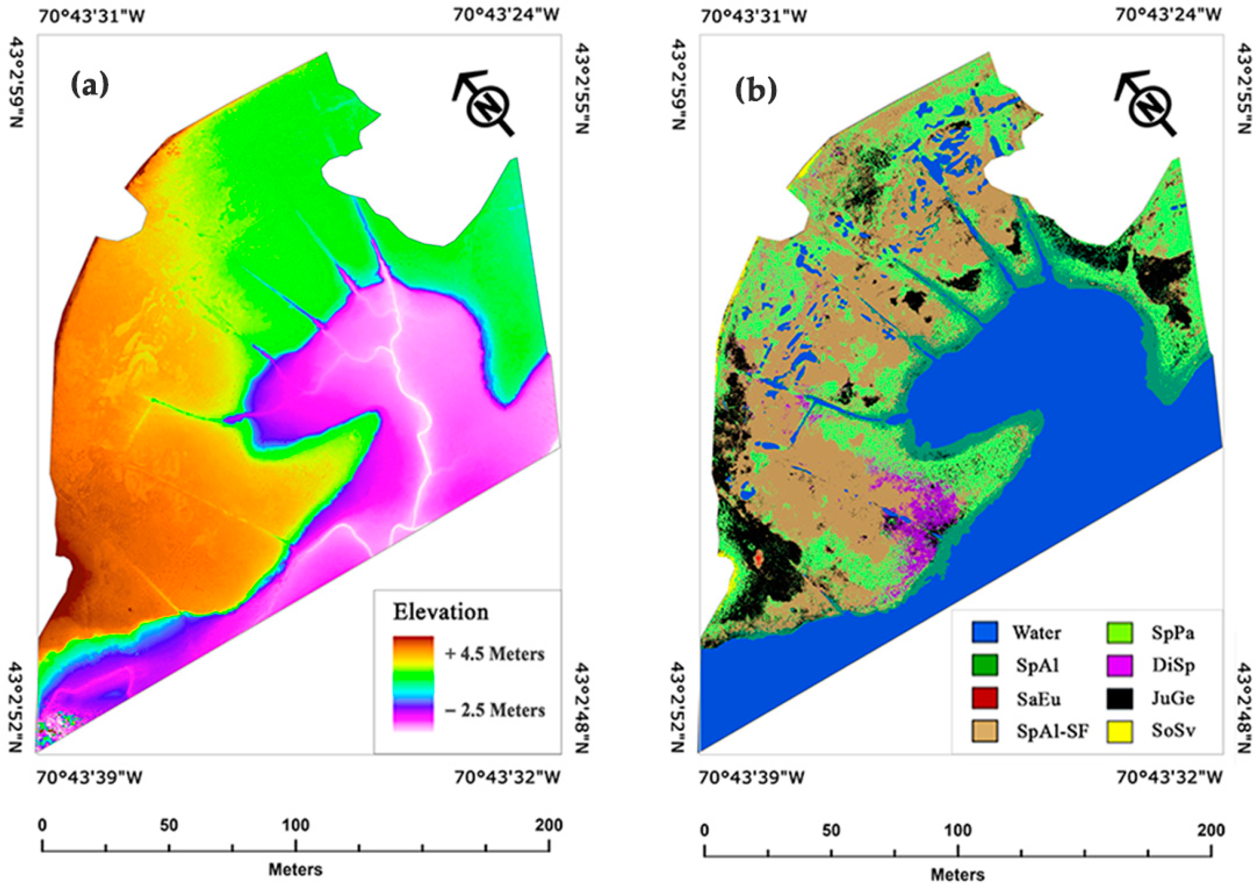
The salt marsh vegetation base elevation profile that we created for study area 2 (Figure 8) and utilized within our RGBD and RGND classifications did not fully follow the same elevation order of plant species as the base elevation profile created for study area 1 (Figure 5) or that of salt marshes study within the nearby Great Bay Estuary region of New Hampshire, approximately 24 km (15 mi) up the Piscataqua River from our sampling locations [61]. Although SpAl and SoSv were found at the extreme ends of the marsh profile as in study area 1, SaEu, SpAl-SF, SpPa, DiSp, and JuGe were ordered by mean base elevation differently from their counterparts in study area 1. We speculate that this is due to human-made changes in the elevation of the marsh caused by the creation of Rt. 1A, which contains the upper marsh border of this study area. These changes in the base elevation might have altered the freshwater inputs to the marsh, thus having effects on growing zones within the study area, but this speculation needs further study. However, alterations to fresh water inputs into coastal marsh lands have previously been shown to play a role in levels of plant stress and seed generation and growth [103], factors that can alter plant cover. We also speculate that the Rt. 1A bridge adjacent to study area 2 may be the source of a tidal restriction that forces water to build up behind it during large ebb tides. This, in turn, may be altering the normal base elevations of growing zones within this area, but this speculation also needs further study. However, our current data show that SaEu, a plant that often can live along low-lying shallow salt pans, resided at a much higher base elevation relative to its neighboring vegetation types in study area 2 than in study area 1 (Figure 8). Furthermore, the nearly double UAV SfM-derived DEM vertical RMS accuracy of 10.68 cm (4.2 in) in study area 2 vs. 4.60 cm (1.81 in) in study area 1 likely further confounded the study area 2 RGBD and RGND classifications, resulting in their lower classification accuracies (Table 5a and Table 6a). We suspect that the differing vertical RMS results of the two study areas are due to study area 2 having a more complex landscape with more varying and steeper drop-offs at the water line and more deep holes and ditches over the landscape as compared to study area 1. The more complex ground features of study area 2, as captured from our nadir-acquired imagery, were likely harder for SfM to resolve into an accurate DEM than our less complex study area 1 ground features. Previous research shows that the capture of more complex landscapes can be better resolved, with the inclusion of both nadir and off-nadir-acquired imagery, into SfM processing [104]. We also acknowledge that the use of an RTK positioning-enabled drone may also help to increase the RMS accuracies of the collection of future elevation layers [105].

Despite variations in the ordering of species’ base elevations between study areas 1 and 2, they both support the influence that regular tidal flooding and the mean-high-tide (MHT) line may have on the break line between the low-marsh growing zone, dominated nearly exclusively by the species SpAl, and the high-marsh growing zone that contains the other species we studied within our research. Study area 2 has an SpAl base elevation of 1.27 m, which is 0.03 m lower than the 1.3 m MHT line recorded 4 km away at the Fort Point NOAA gauging station [86]. Study area 1 has an SpAl base elevation of 1.12 m, which is 0.18 m lower than the 1.3 MHT line [86] recorded 5 km away at the Fort Point NOAA gauging station [86]. We speculate that the lower SpAl base elevation in study area 1 vs. study area 2 may be due to their differences in distance from the NOAA gauging station and the additional tidal damping effects that study area 1 may experience because it is 1 km deeper into the marsh than study area 2. However, further research also needs to be completed to test these speculations.

4.2.6. A Finer Discussion of Confusion Matrices by Acquisition Date

A review of the study area 1 and 2 confusion matrices by the acquisition date also revealed interesting findings (Appendix A). Though UAs and PAs varied by date, in study area 1, in general, the lowest UAs and PAs were created by the 31 August classifications (Table A1a, Table A2a, Table A3a and Table A4a), and the highest were created by the 1 October classifications (Table A1c, Table A2c, Table A3c and Table A4c), with some slight variations created in the 17 September and 12 October classifications (Table A1b,d, Table A2b,d, Table A3b,d and Table A4b,d). In study area 2, in general, the lowest UAs and PAs were created by the 14 September (Table A5a, Table A6a, Table A7a and Table A8a) and October 14 (Table A5c, Table A6c, Table A7c and Table A8c) classifications, and the highest were created by the 30 September classifications (Table A5b, Table A6b, Table A7b and Table A8b). For instance, though the UAs and PAs of SaEu varied by composite type, they peaked in study area 1 within the 1 October classification (Table A1c, Table A2c, Table A3c and Table A4c) and within the 30 September classification for study area 2 (Table A5b, Table A6b, Table A7b and Table A8b). These peaks in accuracy for SaEu correspond with visual observations of when the plants’ spectral reflectance transitions in color from green to bright red within our study areas, displaying similar color characteristics as those described by Bertness (1992) [36]. Additionally, though the UAs and PAs for SoSv were relatively poor for the RGB (Table A1a–d and Table A5a–c) and RGN (Table A2a–d and Table A6a–c) composites across all the dates, these accuracies increased within the RGBD (Table A3a–d and Table A7a–c) and RGND (Table A4a–d and Table A8a–c) classifications across all the dates. These findings were not unexpected, as the addition of the digital elevation model likely helped to better classify SoSv at its higher base elevation than other species in our study area. Furthermore, it is notable that the UAs and PAs for SpPa and DiSp peaked in the study area 1 (1 October) and study area 2 (30 September) RGND (Table A1c, Table A2c, Table A3c, Table A4c and Table A8a–c) classifications. These findings correspond with in-field observations that revealed that SpPa gained a slight orange hue and DiSp gained a slight purple hue across the landscape around the beginning of October. This phenomenon was the most evident in larger homogeneous patches of the two species. These findings help to support that the spectral reflectance of the marsh species assessed within our study varies through late summer and early fall. These are in line with the in-field hyperspectral analysis findings of Gilmore et al. (2010) [59] but vary somewhat from the findings of Nardin et al. (2021) [67], which showed seasonal color variability within low-marsh species in the fall but persistent green foliage in the high-marsh species, SpPa (also known as Sporobolus pumilus in their study), at the same time of the year in Maryland, USA. With this said, relatively high CCC percentages between our SpPa and DiSp classes for the 1 October (study area 1) and 30 September (study area 2) RGND composite (Table A4c and Table A8b) reveal the difficulty in accurately classifying these species, even at this time of the year, within our study areas. 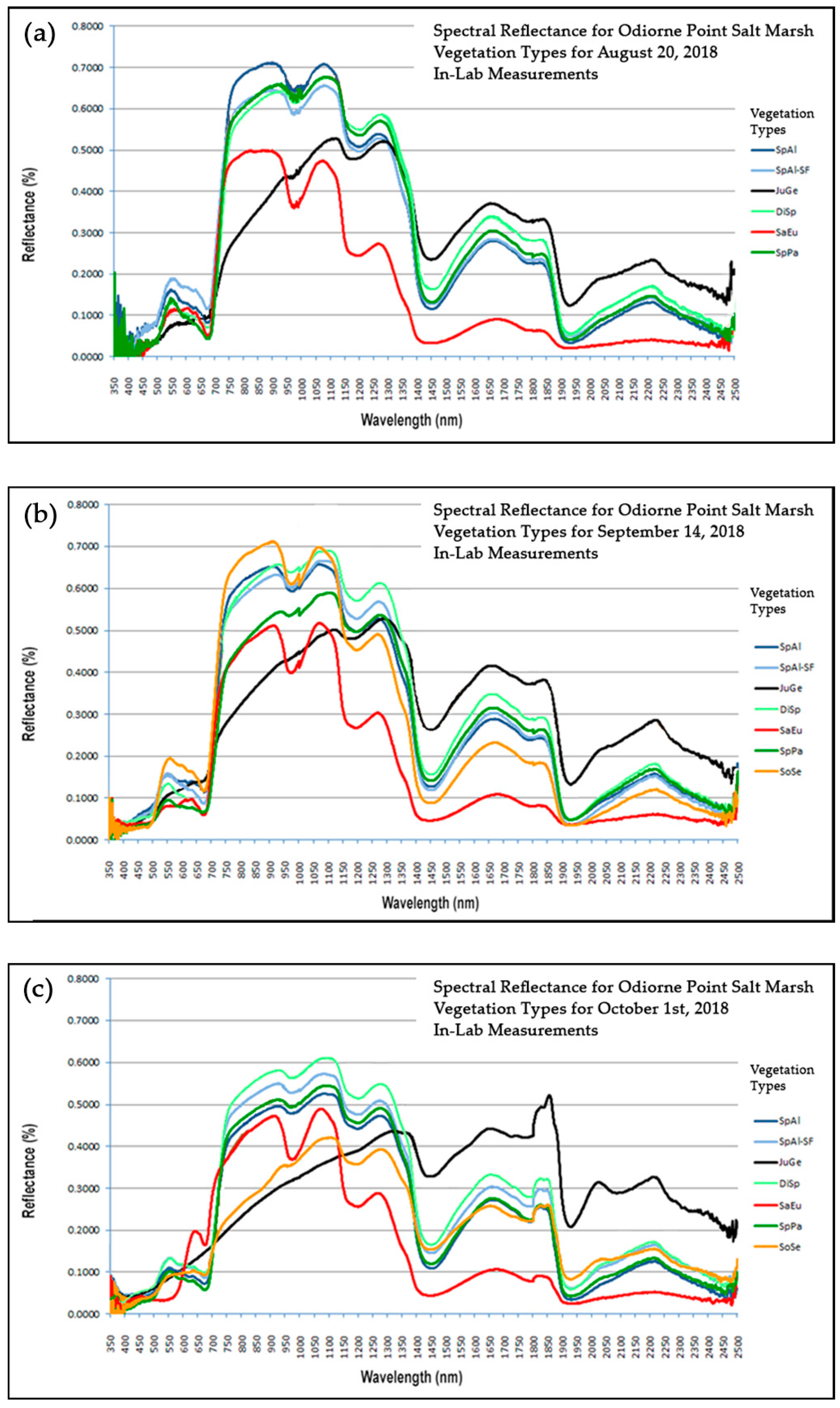Although Artigas and Yang (2006) [77] showed that hyperspectral lab measurements of SpPa and DiSp were more successfully discriminated with the use of near-infrared bands than blue and green bands, we believe that the interwoven co-habitation of these two species in parts of the study area probably confused the maximum likelihood classifier. The calculation of varying TAs, UAs, and PAs occurring across the time period of our study supports hypothesis 3 of this research that UAV-derived vegetation classification total accuracies within our study areas will vary over late summer and early fall. Closer assessments also show that there are variations in user, producer, and CCC accuracies between the classification dates. Furthermore, the variations in the separation of our species spectral curves over late summer and early fall (Figure 2a–c) imply that our project’s classifier capability to render accurate classifications will vary as well, further providing support for hypothesis 3 of this research.

4.3. Methodological Limitations and Next Steps

Within this research, our methodologies utilized a low-cost consumer-grade DJI Phantom 4 Pro UAV equipped with a fixed DJI, red, green, and blue (RGB) camera and a low-cost MapIR, red, green, and near-infrared (RGN) Survey 3 camera for imagery capture. This equipment was used to stay within our project budget and assess the potential of these low-cost sensors for producing accurate classifications. However, this methodology did introduce limitations to our study. For instance, the DJI and MapIR cameras utilized different focal lengths and, thus, produced different pixel sizes. Additionally, although the DJI camera does not have published spectral ranges for its bands, it is possible that its red and green bands do not have the same spectral range as those of the same bands of the MapIR camera. These differences in the characteristics of the two cameras may have influenced the outcomes of our classifications and our accuracy assessments. Thus, they might be a commentary on the cameras’ effectiveness and not just the broad spectral bands they measured. However, with the MapIR camera composite classifications outperforming the DJI camera composite classifications, it is clear that classification accuracies can be significantly improved for only a $400 MapIR camera upgrade. More expensive alternatives to our two-camera approach may include multispectral sensors that capture blue, green, red, and near-infrared bands within the same camera, such as MicaSense cameras ranging from ~$5000 to $12,000. These cameras also provide a downwelling light sensor to compensate for changes in light conditions during a mission, a capacity we could not take advantage of within our study. Furthermore, although not used within our assessment, spectral indices, such as the normalized difference vegetation index (NDVI), could have been created from in situ bands for further testing. However, for this study, we looked to maintain band independence between the layers within our composites so that we could compare how the use of only the basic spectral bands affected composite classification accuracies. However, we do recognize that the assessment of such indices for salt marsh classification accuracies may be fruitful for future research.

Another limitation of our work is that we only utilized two small patch areas within a single salt marsh along the New Hampshire seacoast. This begs the question of how scalable our results are relative to the larger New Hampshire salt marsh system. Although our work only assessed seven dominant plant species within our study areas, our research has demonstrated the ability of our spectral band, elevation layer, and collection date combinations to distinguish specific species from one another. For instance, the use of a DEM layer allowed SpAl vs. SpAl-SF and SpAl vs. SoSv to be more easily distinguished from each other. The use of a NIR layer also allowed for better distinctions between high-marsh species, such as SpPa, DiSp, and JuGe, vs. the low-marsh species SpAl. As these species are prominent throughout many New Hampshire seacoast salt marshes, our research provides a strong foundation for the applicability of our results to other New Hampshire salt marshes. However, varying levels of spectral separability, due to the introduction and mixture of other species within other salt marshes, may alter salt marsh vegetation classification accuracies.

Additionally, although we did not compare object- versus pixel-based analysis and various vegetation class granularities within our research, we believe that these areas of study could be fruitful within our study area and warrant future investigations. Furthermore, because tidal and precipitation effects highly influence our study areas, future work is needed to better compensate for the varying effects of moisture within these landscapes.

5. Conclusions

In conclusion, this research has built upon previous remote sensing and field method research to assess how the spectral, elevation, and temporal characteristics of the UAV-derived imagery of salt marshes can affect the accuracy of their vegetation classifications. We found that the use of a red, green, and near-infrared (RGN) UAV-derived image composite helped to improve classification accuracies over those of red, green, and blue (RGB) true-color imagery composites alone. Finer assessments of cross-class confusions (CCCs), user accuracies (UAs), and producer accuracies (PAs) provided us with additional insights into the dynamics of why classification total accuracies differed from each other. We also found that adding a digital elevation model (DEM) layer to UAV-derived imagery improved the imagery’s classification total accuracies. Closer inspection of the marsh elevations over our two study areas provided further understanding of how species distributions may be affected by variations in the base profile of a marsh. Furthermore, we found that UAV-derived vegetation classification total accuracies did vary over the late summer and early fall in our two study areas, peaking at around the beginning of October. Although these methods were assessed within our two study areas ranging over a series of dates and two growing seasons, we recognize that our findings are influenced by marsh species compositions, base elevation profiles, and seasonal phenological conditions that may vary in other study areas for other growing seasons. Owing to these facts, we attest to the classification accuracies found within our study areas for the time periods that were assessed but believe that the results provided herein can help other researchers to find the best dates and composite layers to help accurately classify plant species within other salt marsh landscapes for time periods of their choosing. These assessments may, in turn, help to provide insights and knowledge into what drivers are affecting change within these environments. Armed with this knowledge, decision-makers can be better equipped to set policy with regard to these important coastal ecosystems.

References

1. Adam, P. Saltmarsh Ecology; Cambridge University Press: New York, NY, USA, 1990. [Google Scholar]
2. Levin, L.A.; Boesch, D.F.; Covich, A.; Dahm, C.; Erseus, C.; Ewel, K.C.; Kneib, R.T.; Moldenki, A.; Palmer, M.A.; Snelgrove, P.; et al. The function of marine critical transition zones and the importance of sediment biodiversity. Ecosystems 2001, 4, 430–451. [Google Scholar] [CrossRef]
3. Gedan, K.B.; Silliman, B.R.; Bertness, M.D. Centuries of human-driven change in salt marsh ecosystems. Annu. Rev. Mar. Sci. 2009, 1, 117–141. [Google Scholar] [CrossRef]
4. Minello, T.; Able, K.; Weinstein, M.; Hays, C.; Minello, T. Salt marshes as nurseries for nekton: Testing hypotheses on density, growth, and survival through meta-analysis. Mar. Ecol. Prog. Ser. 2003, 246, 39–59. [Google Scholar] [CrossRef]
5. Turner, R. Intertidal Vegetation and Commercial Yields of Penaeid Shrimp. Trans. Am. Fish. Soc. 1977, 106, 411–416. [Google Scholar] [CrossRef]
6. Barrett, B.B. Environmental conditions relative to shrimp production in coastal Louisiana. La. Dep. Wildl. Fish. Tech. Bull. 1975, 15, 1–22. [Google Scholar]
7. Nixon, S. The Ecology of New England High Salt Marshes: A Community Profile (Spartina), U.S. Fish & Wildlife Service, Dept. of the Interior; USGS Publications Warehouse: Reston, VA, USA, 1982; Volume 16. [Google Scholar]
8. Tiner, R.W. Wetlands of the United States: Current Status and Trends; US Fish and Wildlife Service, National Wetlands Inventory: Washington, DC, USA, 1984; pp. 15–16.
9. Zimmerman, R.; Minello, T. Densities of Penaeus aztecus, Penaeus setiferus, and other natant macrofauna in a Texas salt marsh. Estuaries 1984, 7, 421–433. [Google Scholar] [CrossRef]
10. Knutson, P.; Brochu, R.; Seelig, W.; Inskeep, M. Wave damping in Spartina alterniflora marshes. Wetlands 1982, 2, 87–104. [Google Scholar] [CrossRef]
11. Miller, C.D. Predicting the impact of vegetation on storm surges. In Wetland Hydrology; Kusler, J.A., Brooks, G., Eds.; Association of State Wetland Managers Technical Report 6; Association of State Wetland Managers: New York, NY, USA, 1988; pp. 113–121. [Google Scholar]
12. Davy, A.J.; Bakker, P.; Figueroa, M.E. Human Modification of European Salt Marshes. In Human Impacts on Salt Marshes: A Global Perspective; Silliman, B.R., Grosholz, E.D., Bertness, M.D., Eds.; University of California Press: Oakland, CA, USA, 2009. [Google Scholar]
13. Lonard, J.F.W.; Stalter, R. The Biological Flora of Coastal Dunes and Wetlands: Spartina patens. J. Coast. Res. 2010, 26, 935–946. [Google Scholar] [CrossRef]
14. Valiela, I.; Teal, J.M. The nitrogen budget of a salt marsh ecosystem. Nature 1979, 280, 652–656. [Google Scholar] [CrossRef]
15. Mitsch, W.J.; Gosselink, J.G. Wetlands; Van Nostrand Reinhold: New York, NY, USA, 2008. [Google Scholar]
16. Chmura, G.; Anisfeld, S.; Cahoon, D.; Lynch, J. Global carbon sequestration in tidal, saline wetland soils. Glob. Biogeochem. Cycles 2003, 17. [Google Scholar] [CrossRef]
17. Nelson, J.; Zavaleta, E.; Cebrian, J. Salt Marsh as a Coastal Filter for the Oceans: Changes in Function with Experimental Increases in Nitrogen Loading and Sea-Level Rise. PLoS ONE 2012, 7, e38558. [Google Scholar] [CrossRef] [PubMed]
18. Burdick, D.M.; Peter, C.R.; Feurt, C.; Fischella, B.; Tyrrell, M.; Allen, J.; Goldstein, J.; Raposa, K.; Mora, J.; Crane, L. Synthesizing NERR Sentinel Site Data to Improve Coastal Wetland Management across New England; National Science Collaborative: Durham, NH, USA, 2020. [Google Scholar]
19. IPCC. IPCC Climate Change 2014: Synthesis Report. Contribution of Working Groups I, II, and III to the Fifth Assessment Report of the Intergovernmental Panel on Climate Change; Core Writing Team, Pachauri, R.K., Meyer, L.A., Eds.; IPCC: Geneva, Switzerland, 2014. [Google Scholar]
20. USGCRP. Climate Science Special Report: Fourth National Climate Assessment, Volume I; Wuebbles, D.J., Fahey, D.W., Hibbard, K.A., Dokken, D.J., Stewart, B.C., Maycock, T.K., Eds.; U.S. Global Change Research Program: Washington, DC, USA, 2017; p. 470. [Google Scholar]
21. Cahoon, D.R.; Guntenspergen, G.R. Climate Change, Sea-Level Rise, and Coastal Wetlands, National Wetlands Newsletter; Environmental Law Institute: Washington, DC, USA, 2010; Volume 32. [Google Scholar]
22. Bromberg, K.; Bertness, M. Reconstructing New England salt marsh losses using historical maps. Estuaries 2005, 28, 823–832. [Google Scholar] [CrossRef]
23. Gosselink, J.; Baumann, R. Wetland inventories: Wetland loss along the United States coast. Z. Fur Geomorphol. Suppl. 1980, 34, 173–187. [Google Scholar]
24. Deegan, L.; Johnson, D.; Warren, R.; Peterson, B.J.; Fleeger, J.B.; Fagherazzi, S.; Wollheim, W.M. Coastal eutrophication as a driver of salt marsh loss. Nature 2012, 490, 388–392. [Google Scholar] [CrossRef] [PubMed]
25. Montague, C.; Zale, A.; Percival, H. Ecological effects of coastal marsh impoundments: A review. Environ. Manag. 1987, 11, 743–756. [Google Scholar] [CrossRef]
26. Moore, G.; Konisky, R.; Burdick, D. Fresh Creek Tidal Restriction and Restoration Potential Assessment: Final Report; New Hampshire Coastal Program: Portsmouth, NH, USA, 2010. [Google Scholar]
27. Mora, J.; Burdick, D. The impact of man-made earthen barriers on the physical structure of New England tidal marshes (USA). Wetl. Ecol. Manag. 2013, 21, 387–398. [Google Scholar] [CrossRef]
28. Burdick, D.M. Evaluation of Pre-Restoration Conditions, Including Impacts from Tidal Restriction, in Little River Marsh, New Hampshire; Jackson Estuarine Laboratory, Dept. of Natural Resources University of New Hampshire: Durham, NH, USA, 2002. [Google Scholar]
29. Burdick, D.; Dionne, M.; Boumans, R.; Short, F. Ecological responses to tidal restorations of two northern New England salt marshes. Wetl. Ecol. Manag. 1997, 4, 129–144. [Google Scholar] [CrossRef]
30. Anisfeld, S.; Benoit, G. Impacts of flow restrictions on salt marshes: An instance of acidification. Environ. Sci. Technol. 1997, 31, 1650–1657. [Google Scholar] [CrossRef]
31. Boumans, R.M.J.; Burdick, D.M.; Dionne, M. Modeling Habitat Change in Salt Marshes after Tidal Restoration. Restor. Ecol. 2002, 10, 543–555. [Google Scholar] [CrossRef]
32. Eleuterius, L.; Eleuterius, C.; Getsen, M. Tide levels and salt marsh zonation. Bull. Mar. Sci. 1979, 29, 394–400. [Google Scholar]
33. Lefor, M.W.; Kennard, W.C.; Civco, D.L. Relationships of salt-marsh plant distributions to tidal levels in Connecticut, USA. Environ. Manag. 1987, 11, 61. [Google Scholar] [CrossRef]
34. McKee, K.; Patrick, W. The relationship of smooth cordgrass (Spartina alterniflora) to tidal datums: A review. Estuaries 1988, 11, 143–151. [Google Scholar] [CrossRef]
35. Hickey, D.; Bruce, E. Examining tidal inundation and salt marsh vegetation distribution patterns using spatial analysis (Botany Bay, Australia). J. Coast. Res. 2010, 26, 94–102. [Google Scholar] [CrossRef]
36. Bertness, M.D. The Ecology of a New England Salt Marsh. Am. Sci. 1992, 80, 260–268. [Google Scholar]
37. Pennings, S.; Bertness, M. Plant zonation in low-latitude salt marshes: Disentangling the roles of flooding, salinity, and competition. J. Ecol. 2005, 93, 159–167. [Google Scholar] [CrossRef]
38. Valiela, I.; Teal, J.; Valiela, I. Nutrient Limitation in Salt Marsh Vegetation. Ecology of Halophytes; Reimold, R.J., Queen, W.H., Eds.; Academic Press, Inc.: New York, NY, USA, 1975; pp. 547–563. [Google Scholar]
39. Theodose, T.; Martin, J. Microclimate and substrate quality controls on nitrogen mineralization in a New England high salt marsh. Plant Ecol. 2003, 167, 213–221. [Google Scholar] [CrossRef]
40. Gleason, M.; Zieman, J. Influence of tidal inundation on internal oxygen supply of Spartina alterniflora and Spartina patens. Estuar. Coast. Shelf Sci. 1981, 13, 47–57. [Google Scholar] [CrossRef]
41. Minchinton, T.; Simpson, J.; Bertness, M. Mechanisms of exclusion of native coastal marsh plants by an invasive grass. J. Ecol. 2006, 94, 342–354. [Google Scholar] [CrossRef]
42. Warren, R.S.; Niering, W.A. Vegetation change on a northeast tidal marsh: Interaction of sea-level rise and marsh accretion. Ecology 1993, 74, 96–103. [Google Scholar] [CrossRef]
43. Donnelly, J.P.; Bertness, M.D. Rapid shoreward encroachment of salt marsh cordgrass in response to accelerated sea-level rise. Proc. Natl. Acad. Sci. USA 2001, 98, 14218–14223. [Google Scholar] [CrossRef]
44. Smith, S.M. Multi-decadal Changes in Salt Marshes of Cape Cod, MA: Photographic Analyses of Vegetation Loss, Species Shifts, and Geomorphic Change. Northeast. Nat. 2009, 16, 183–208. [Google Scholar] [CrossRef]
45. Smith, S.M. Vegetation Change in Salt Marshes in Cape Cod National Seashore (Massachusetts, USA) Between 1984 and 2013. Wetlands 2015, 35, 127–136. [Google Scholar] [CrossRef]
46. Watson, E.; Szura, K.; Wigand, C.; Raposa, K.; Blount, K.; Cencer, M. Sea level rise, drought and the decline of Spartina patens in New England marshes. Biol. Conserv. 2016, 196, 173–181. [Google Scholar] [CrossRef]
47. Bertness, M.D. Zonation of Spartina patens and Spartina alterniflora in a New England salt marsh. Ecology 1991, 72, 138–148. [Google Scholar] [CrossRef]
48. Civco, D.L.; Kennard, W.C.; Lefor, M.W. Changes in Connecticut salt-marsh vegetation as revealed by historical aerial photographs and computer-assisted cartographics. Environ. Manag. 1986, 1, 229. [Google Scholar] [CrossRef]
49. Belluco, E.; Camuffo, M.; Ferrari, S.; Modenese, L.; Silvestri, S.; Marani, A.; Marani, M. Mapping salt-marsh vegetation by multispectral and hyperspectral remote sensing. Remote Sens. Environ. 2006, 105, 54–67. [Google Scholar] [CrossRef]
50. Sun, C.; Fagherazzi, S.; Liu, Y. Classification mapping of salt marsh vegetation by flexible monthly NDVI time-series using Landsat imagery. Estuar. Coast. Shelf Sci. 2018, 213, 61–80. [Google Scholar] [CrossRef]
51. Wang, X.; Gao, X.; Zhang, Y.; Fei, X.; Chen, Z.; Wang, J.; Zhang, Y.; Lu, X.; Zhao, H. Land-Cover Classification of Coastal Wetlands Using the RF Algorithm for Worldview-2 and Landsat 8 Images. Remote Sens. 2019, 11, 1927. [Google Scholar] [CrossRef]
52. McKown, J.G.; Moore, G.E.; Payne, A.R.; White, N.A.; Gibson, J.L. Successional dynamics of a 35-year-old freshwater mitigation wetland in southeastern New Hampshire. PLoS ONE 2021, 16, e0251748. [Google Scholar] [CrossRef]
53. Moore, G.E.; Burdick, D.M.; Routhier, M.R.; Novak, A.B.; Payne, A.R. Effects of a large-scale, natural sediment deposition event on plant cover in a Massachusetts salt marsh. PLoS ONE 2021, 16, e0245564. [Google Scholar] [CrossRef]
54. Harvey, K.R.; Hill, J.E. Vegetation mapping of a tropical freshwater swamp in the Northern Territory, Australia: A comparison of aerial photography, Landsat TM and SPOT satellite imagery. Remote Sens. Environ. 2001, 22, 2911–2925. [Google Scholar] [CrossRef]
55. McCarthy, J.; Gumbricht, T.; McCarthy, T.S. Ecoregion classification in the Okavango Delta, Botswana from multitemporal remote sensing. Int. J. Remote Sens. 2005, 26, 4339–4357. [Google Scholar] [CrossRef]
56. Elhadi, A.; Mutanga, O.; Rugege, D. Multispectral and hyperspectral remote sensing for identification and mapping of wetland vegetation: A review. Wetl. Ecol Manag. 2010, 18, 281–296. [Google Scholar]
57. Sun, C.; Li, J.; Liu, Y.; Liu, Y.; Liu, R. Plant species classification in salt marshes using phenological parameters derived from Sentinel-2 pixel-differential time-series. Remote Sens. Environ. 2021, 256, 112320. [Google Scholar] [CrossRef]
58. Schmidt, K.S.; Skidmore, A.K. Spectral discrimination of vegetation types in a coastal wetland. Remote Sens. Environ. 2003, 85, 92–108. [Google Scholar] [CrossRef]
59. Gilmore, M.; Civco, D.; Wilson, E.; Barrett, N.; Prisloe, S.; Hurd, J.; Chadwick, C. Remote Sensing and In Situ Measurements for Delineation and Assessment of Coastal Marshes and Their Constituent Species. In Remote Sensing of Coastal Environments; Taylor & Francis Group: Boca Raton, FL, USA, 2010; pp. 261–280. [Google Scholar]
60. Correll, M.D.; Hantson, W.; Hodgman, T.P.; Cline, B.B.; Elphick, C.S.; Shriver, W.G.; Tymkiw, E.L.; Olsen, B.J. Fine-Scale Mapping of Coastal Plant Communities in the Northeastern USA. Wetlands 2019, 39, 17–28. [Google Scholar] [CrossRef]
61. Stevens, R.A.; Carter, H.J.; Peter, C.R. An Ecological Approach to Designing Salt Marshes. Tidal Wetland Vegetation Elevation and Ecotone Boundaries in Great Bay, New Hampshire. Great Bay National Estuarine Research Reserve Technical Report; Great Bay National Estuarine Research Reserve: Greenland, NH, USA, 2022; Volume 24. [Google Scholar]
62. USGS, USGS EROS Archive—Aerial Photography—National Agriculture Imagery Program (NAIP), Earth Observation and Science (EROS) Center. 2018. Available online: https://www.usgs.gov/centers/eros/science/usgs-eros-archive-aerial-photography-national-agriculture-imagery-program-naip#overview (accessed on 1 April 2023).
63. Anderson, K.; Gaston, K.J. Lightweight unmanned aerial vehicles will revolutionize spatial ecology. Front. Ecol. Environ. 2013, 11, 138–146. [Google Scholar] [CrossRef]
64. Manfreda, S.; McCabe, M.F.; Miller, P.E.; Lucas, R.; Pajuelo Madrigal, V.; Mallinis, G.; Ben-Dor, E.; Helman, D.; Estes, L.; Ciraolo, G.; et al. On the Use of Unmanned Aerial Systems for Environmental Monitoring. Remote Sens. 2018, 10, 641. [Google Scholar] [CrossRef]
65. Ierodiaconou, D.; Schimel, A.C.G.; Kennedy, D.M. A new perspective of storm bite on sandy beaches using unmanned aerial vehicles. Z. Für Geomorphol. 2016, 60, 123–137. [Google Scholar] [CrossRef]
66. Casella, E.; Collin, A.; Harris, D.; Ferse, S.; Bejarano, S.; Parravicini, V.; Hench, J.L.; Rovere, A. Mapping coral reefs using consumer-grade drones and structure from motion photogrammetry techniques. Coral Reefs 2017, 36, 269–275. [Google Scholar] [CrossRef]
67. Nardin, W.; Taddia, Y.; Quitadamo, M.; Vona, I.; Corbau, C.; Franchi, G.; Staver, L.W.; Pellegrinelli, A. Seasonality and Characterization Mapping of Restored Tidal Marsh by NDVI Imageries Coupling UAVs and Multispectral Camera. Remote Sens. 2021, 13, 4207. [Google Scholar] [CrossRef]
68. Collin, A.; Lambert, N.; Etienne, S. Satellite-based salt marsh elevation, vegetation height, and species composition mapping using the superspectral WorldView-3 imagery. Int. J. Remote Sens. 2018, 39, 5619–5637. [Google Scholar] [CrossRef]
69. Zhou, Z.; Yang, Y.; Chen, B. Estimating Spartina alterniflora fractional vegetation cover and aboveground biomass in a coastal wetland using SPOT6 satellite and UAV data. Aquat. Bot. 2018, 114, 38–45. [Google Scholar] [CrossRef]
70. Zhu, X.; Meng, L.; Zhang, Y.; Weng, Q.; Morris, J. Tidal and Meteorological Influences on the Growth of Invasive Spartina alterniflora: Evidence from UAV Remote Sensing. Remote Sens. 2019, 11, 1208. [Google Scholar] [CrossRef]
71. Oldeland, J.; Revermann, R.; Luther-Mosebach, J.; Buttschardt, T.; Lehmann, J.R.K. New tools for old problems—Comparing drone- and field-based assessments of a problematic plant species. Environ. Monit. Assess. 2021, 193, 90. [Google Scholar] [CrossRef]
72. Curcio, A.C.; Barbero, L.; Peralta, G. UAV-Hyperspectral Imaging to Estimate Species Distribution in Salt Marshes: A Case Study in the Cadiz Bay (SW Spain). Remote Sens. 2023, 15, 1419. [Google Scholar] [CrossRef]
73. Doughty, C.; Cavanaugh, K. Mapping Coastal Wetland Biomass from High-Resolution Unmanned Aerial Vehicle (UAV) Imagery. Remote Sens. 2019, 11, 540. [Google Scholar] [CrossRef]
74. Kalacska, M.; Chmura, G.L.; Lucanus, O.; Bérubé, D.; Arroyo-Mora, J.P. Structure from motion will revolutionize analyses of tidal wetland landscapes. Remote Sens. Environ. 2017, 199, 14–24. [Google Scholar] [CrossRef]
75. Baena, S.; Moat, J.; Whaley, O.; Boyd, D. Identifying species from the air: UAVs and the very high-resolution challenge for plant conservation. PLoS ONE 2017, 12, e0188714. [Google Scholar] [CrossRef]
76. Grybas, H.; Congalton, R.G. Comparison of Multi-Temporal RGB and Multispectral UAS Imagery for Tree Species Classification in Heterogeneous New Hampshire Forests. Remote Sens. 2021, 13, 2631. [Google Scholar] [CrossRef]
77. Artigas, F.J.; Yang, J. Spectral Discrimination of Marsh Vegetation Types in the New Jersey Meadowlands, USA. Wetlands 2006, 26, 271–277. [Google Scholar] [CrossRef]
78. Lee, D.; Shan, J. Combining Lidar Elevation Data and IKONOS Multispectral Imagery for Coastal Classification Mapping. Mar. Geod. 2003, 26, 117–127. [Google Scholar] [CrossRef]
79. Fraser, B.; Congalton, R. Issues in Unmanned Aerial Systems (UAS) Data Collection of Complex Forest Environments. Remote Sens. 2018, 10, 908. [Google Scholar] [CrossRef]
80. Suir, G.M.; Saltus, C.L.; Sasser, C.E.; Harris, J.M.; Reif, M.K.; Diaz, R.; Giffin, B. Evaluating Drone Truthing as an Alternative to Ground Truthing: An Example with Wetland Plant Identification; ERDC/TN APCRP-MI-9; Environmental Laboratory (U.S.): Vicksburg, MS, USA, 2021. [Google Scholar]
81. NOAA, Tides and Currents, Datums for 8423898, Fort Point NH. 2023. Available online: https://tidesandcurrents.noaa.gov/datums.html?datum=MSL&units=1&epoch=0&id=8423898&name=Fort+Point&state=NH (accessed on 10 January 2023).
82. Malvern Panalytics, 2018, ASD FieldSpec 4 Hi-Res: High Resolution Spectroradiometer Specifications, Malvern Panalytics. Available online: https://www.malvernpanalytical.com/en/products/product-range/asd-range/fieldspec-range/fieldspec4-hi-res-high-resolution-spectroradiometer#specs (accessed on 12 October 2023).
83. Montana, J.M.; Torres, R. Accuracy assessment of lidar saltmarsh topographic data using RTK GPS. Photogramm. Eng. Remote Sens. 2006, 72, 961–967. [Google Scholar] [CrossRef]
84. Morris, J.T.; Porter, D.; Neet, M.; Noble, P.A.; Schmidt, L.; Lapine, L.A.; Jensen, J.R. Integrating LIDAR elevation data, multispectral imagery and neural network modeling for marsh characterization. Int. J. Remote Sens. 2005, 26, 5221–5234. [Google Scholar] [CrossRef]
85. Schmid, K.A.; Hadley, B.C.; Wijekoon, N. Vertical Accuracy and Use of Topographic LIDAR Data in Coastal Marshes. J. Coast. Res. 2011, 27, 116–132. [Google Scholar] [CrossRef]
86. Rogers, J.N.; Parrish, C.E.; Ward, L.G.; Burdick, D.M. Assessment of Elevation Uncertainty in Salt Marsh Environments using Discrete-Return and Full-Waveform Lidar. J. Coast. Res. 2016, 76, 107–122. [Google Scholar] [CrossRef]
87. DJI. Phantom 4 Pro/Pro+ User Manual, version 1.0; DJI: Shenzhen, China, 2016.
88. Agisoft. Agisoft Metashape User Manual Professional Edition, version 1.6; Agisoft LLC: St. Petersburg, Russia, 2020.
89. ESRI. About ArcGIS Pro; ESRI: Redland, CA, USA, 2021; Available online: https://pro.arcgis.com/en/pro-app/2.6/get-started/get-started.htm (accessed on 12 October 2023).
90. Trimble, Inc. Trimble R10 GNSS RECEIVER, version 1.10; Revision C: Sunnyvale, CA, USA, 2015.
91. MAPIR, Inc. Survey3 Camera Datasheet, version 3.0; MAPIR, Inc.: San Diego, CA, USA, 2018.
92. Congalton, R.G.; Green, K. Assessing the Accuracy of Remotely Sensed Data: Principles and Practices; CRC Press: Boca Raton, FL, USA, 2009; Volume 3. [Google Scholar]
93. Congalton, R.G. A Review of Assessing the Accuracy of Classifications of Remotely Sensed Data. Remote Sens. Environ. 1991, 37, 35–46. [Google Scholar] [CrossRef]
94. NHView. User’s Guide for the Visual Basic (VB6) Version of the MARGFIT and KAPPA Analysis Programs. 2012. Available online: http://www.nhview.unh.edu/pdf/Kappa_Margift_Guides.pdf (accessed on 12 October 2023).
95. Congalton, R.G.; Oderwald, R.G.; Mead, R.A. Assessing Landsat classification accuracy using discrete multivariate analysis statistical techniques. Photogramm. Eng. Remote Sens. 1983, 49, 1671–1678. [Google Scholar]
96. Lu, B.; He, Y. Species classification using Unmanned Aerial Vehicle (UAV)-acquired high spatial resolution imagery in a heterogeneous grassland. ISPRS J. Photogramm. Remote Sens. 2017, 128, 73–85. [Google Scholar] [CrossRef]
97. Schiefer, F.; Kattenborn, T.; Frick, A.; Frey, J.; Schall, P.; Koch, B.; Schmidtlein, S. Mapping forest tree species in high-resolution UAV-based RGB-imagery by means of convolutional neural networks. ISPRS J. Photogramm. Remote Sens. 2020, 170, 205–215. [Google Scholar] [CrossRef]
98. Kimes, D.S.; Nelson, R.F.; Manry, M.T.; Fung, A.K. Review article: Attributes of neural networks for extracting continuous vegetation variables from optical and radar measurements. Int. J. Remote Sens. 1998, 19, 2639–2663. [Google Scholar] [CrossRef]
99. Chaeli, J.; Steinberg, S.; Shaughnessy, F.; Crawford, G. Mapping Salt Marsh Vegetation using Aerial Hyperspectral Imagery and Linear Unmixing in Humboldt Bay, California. Wetlands 2007, 27, 1144–1152. [Google Scholar]
100. Zhang, Y.; Lu, D.; Yang, B.; Sun, C.; Sun, M. Coastal wetland vegetation classification with a Landsat Thematic Mapper image. Int. J. Remote Sens. 2011, 32, 545–561. [Google Scholar] [CrossRef]
101. Lisein, J.; Michez, A.; Claessens, H.; Lejeune, P. Discrimination of Deciduous Tree Species from Time Series of Unmanned Aerial System Imagery. PLoS ONE 2015, 10, e0141006. [Google Scholar] [CrossRef]
102. WillyWeather. Tide Times and Heights, Berrys Brook and Squamscott River—Railroad Bridge, United States/NH/Rockingham County. 2023. Available online: https://tides.willyweather.com/nh/rockingham-county/squamscott-river--railroad-bridge.html. (accessed on 1 April 2023).
103. Alexander, H.D.; Dunton, K.H. Freshwater Inundation Effects on Emergent Vegetation of a Hypersaline Salt Marsh. Estuaries 2002, 25, 1426–1435. [Google Scholar] [CrossRef]
104. Nesbit, P.; Hugenholtz, C. Enhancing UAV–SfM 3D Model Accuracy in High-Relief Landscapes by Incorporating Oblique Images. Remote Sens. 2019, 11, 239. [Google Scholar] [CrossRef]
105. Chen, C.; Tian, B.; Wu, W.; Duan, Y.; Zhou, Y.; Zhang, C. UAV photogrammetry in intertidal mudflats: Accuracy, efficiency, and potential for integration with satellite imagery. Remote Sens. 2023, 15, 1814. [Google Scholar] [CrossRef]
Figure 1. Map of the project’s two study areas (demarcated in red) at the Odiorne Point Salt Marsh in Rye, New Hampshire, USA. The red star on the locus map represents the location of the project study areas in Rye, New Hampshire.
Remotesensing 15 05076 g001
Figure 2. (ac) Example spectral signature curves for New Hampshire salt marsh vegetation species for the dates of 20 August (a), 14 September (b), and 1 October 2018 (c). (Abbreviations: SpAl: Spartina alterniflora; SpAl-SF: Short form Spartina alterniflora; JuGe: Juncus gerardii; DiSp: Distichlis spicata; SaEu: Salicornia europaea; SpPa: Spartina patens; SoSv: Solidago sempervirens). Note that no SoSv: Solidago sempervirens data was recorded for 20 August 2018.
Remotesensing 15 05076 g002
Figure 3. (ad) Example maps of 1 October 2018 UAV image RGB (a), RGN (b), RGBD (c), and RGND (d) composite classifications for study area 1 at the Odiorne Point Salt Marsh in Rye, New Hampshire, USA. (Composite band codes: R = red; G = green; B = blue; N = near infrared; D = digital elevation model. Non-underlined codes represent bands from a DJI Phantom 4 Pro red, green, and blue imaging camera. Underlined codes represent bands from a MapIR Survey3 red, green, and near-infrared camera. Doubly underlined codes represent a structure from a motion-derived digital elevation model.) (Abbreviations: JuGe = Juncus gerardii, SpPa = Spartina patens, SaEu = Salicornia europaea, SpAl = Spartina alterniflora, SoSv = Solidago sempervirens, DiSp = Distichlis spicata, and SpAl-SF = Spartina alterniflora—short form).
Remotesensing 15 05076 g003
Figure 4. (a,b) Maps of the digital elevation model (ground-level elevation) (a) and the 1 October 2018 RGND (red, green, near infrared, and digital elevation model) composite classification (b) for study area 1. (Abbreviations: JuGe = Juncus gerardii, SpPa = Spartina patens, SaEu = Salicornia europaea, SpAl = Spartina alterniflora, SoSv = Solidago sempervirens, DiSp = Distichlis spicata, and SpAl-SF = Spartina alterniflora—short form).
Remotesensing 15 05076 g004
Figure 5. Chart of vegetation types vs. mean base-level elevations above tidal datum (with standard deviation bars) within study area 1 at the Odiorne Point Salt Marsh study area in Rye, New Hampshire, USA. Data were evaluated with Welch (α = 0.05) and Games–Howell post hoc pairwise comparison tests for vegetation-type pairs. Different letters indicate significant differences in mean ground elevations among vegetation types. (List of p-values for vegetation-type pairs can be found in Appendix B, Table A9). Abbreviations: JuGe = Juncus gerardii, SpPa = Spartina patens, SaEu = Salicornia europaea, SpAl = Spartina alterniflora, SoSv = Solidago sempervirens, DiSp = Distichlis spicata, and SpAl-SF = Spartina alterniflora—short form).
Remotesensing 15 05076 g005
Figure 6. (ad) Example maps of 30 September 2022 UAV image RGB (a), RGN (b), RGBD (c), and RGND (d) composite classifications for study area 2 at the Odiorne Point Salt Marsh in Rye, New Hampshire, USA. (Composite band codes: R = red; G = green; B = blue; N = near infrared; D = digital elevation model. Non-underlined codes represent bands from a DJI Phantom 4 Pro red, green, and blue imaging camera. Underlined codes represent bands from a MapIR Survey3 red, green, and near-infrared camera. Doubly underlined codes represent a structure from motion-derived digital elevation model.) (Abbreviations: JuGe = Juncus gerardii, SpPa = Spartina patens, SaEu = Salicornia europaea, SpAl = Spartina alterniflora, SoSv = Solidago sempervirens, DiSp = Distichlis spicata, and SpAl-SF = Spartina alterniflora—short form).
Remotesensing 15 05076 g006
Figure 7. (a,b) Maps of the digital elevation model (base ground-level elevations) (a) and the 30 September 2022 RGND (red, green, near infrared, and digital elevation model) composite classification (b) for study area 2 (Abbreviations: JuGe = Juncus gerardii, SpPa = Spartina patens, SaEu = Salicornia europaea, SpAl = Spartina alterniflora, SoSv = Solidago sempervirens, DiSp = Distichlis spicata, and SpAl-SF = Spartina alterniflora—short form).
Remotesensing 15 05076 g007
Figure 8. Chart of vegetation types vs. mean elevations (base-level ground elevations) above tidal datum (with standard deviation bars) within study area 2 at the Odiorne Point Salt Marsh study area in Rye, New Hampshire, USA. Data were evaluated with Welch (α = 0.05) and Games–Howell post hoc pairwise comparison tests for vegetation-type pairs. Different letters indicate significant differences in mean base-level ground elevations among the vegetation types. (A list of p-values for vegetation-type pairs can be found in Appendix B, Table A10). (Abbreviations: JuGe = Juncus gerardii, SpPa = Spartina patens, SaEu = Salicornia europaea, SpAl = Spartina alterniflora, SoSv = Solidago sempervirens, DiSp = Distichlis spicata, and SpAl-SF = Spartina alterniflora—short form).
Remotesensing 15 05076 g008