Article

Vegetation Trend Detection Using Time Series Satellite Data as Ecosystem Condition Indicators for Analysis in the Northwestern Highlands of Ethiopia

by
Bireda Alemayehu
1,2,*,
Juan Suarez-Minguez
3,
Jacqueline Rosette
4 and
Saeed A. Khan
5
1
Space Science and Geospatial Institute, Addis Ababa P.O. Box 33679, Ethiopia
2
Department of Geography and Environmental Studies, Debre Markos University, Debre Markos P.O. Box 269, Ethiopia
3
Forest Research Agency of the Forestry Commission, Northern Research Station, Midlothian EH25 9SY, UK
4
Department of Geography, Swansea University, Swansea SA2 8PP, UK
5
Department of Geography, University of Bayreuth, D-95447 Bayreuth, Germany
*
Author to whom correspondence should be addressed.
Remote Sens. 2023, 15(20), 5032; https://doi.org/10.3390/rs15205032
Submission received: 12 August 2023 / Revised: 20 September 2023 / Accepted: 22 September 2023 / Published: 20 October 2023
(This article belongs to the Section Ecological Remote Sensing)

Abstract

:
Vegetation is an essential component of the terrestrial ecosystem and has changed significantly over the last two decades in the Northwestern Highlands of Ethiopia. However, previous studies have focused on the detection of bitemporal change and lacked the incorporation of entire vegetation time series changes, which are considered significant indicators of ecosystem conditions. The Normalized Difference Vegetation Index (NDVI) time series dataset from the Moderate-Resolution Imaging Spectroradiometer (MODIS) is an efficient method for analyzing the dynamics of vegetation change over a lengthy period using remote sensing techniques. This study aimed to utilize time series satellite data to detect vegetation changes from 2000 to 2020 and investigate their links with ecosystem conditions. The time-series satellite processing package (TIMESAT) was used to estimate the seasonal parameter values of NDVI and their correlation across the seasons during the study period. Break Detection for Additive Season and Trend (BFAST) was applied to identify the year of breakpoints, the direction of magnitude, and the number of breakpoints. The results were reported, analyzed, and linked to ecosystem conditions. The overall trend in the study area increased from 0.58 (2000–2004) to 0.65 (2015–2020). As a result, ecosystem condition indicators such as peak value (PV), base value (BV), amplitude (Amp), and large integral (LI) exhibited significant positive trends, particularly for Acacia decurrens plantations, Eucalyptus plantations, and grasslands, but phenology indicator parameters such as start of season (SOS), end of season (EOS), and length of season (LOS) did not show significant trends for almost any vegetation type. The most abrupt changes were recorded in 2015 (24.7%), 2012 (18.6%), and 2014 (9.8%). Approximately 30% of the vegetation changes were positive in magnitude. The results of this study imply that there was an improvement in the ecosystem’s condition following the establishment of the Acacia decurrens plantation. The findings are considered relevant inputs for policymakers and serve as an initial stage for the assessment of the other environmental and climatic implications of Acacia decurrens plantations at the local scale.

1. Introduction

Vegetation is one of the main elements in terrestrial ecosystems [1], and is directly connected to a variety of ecosystem services, such as soil retention, water infiltration, and carbon sequestration [2]. Through the process of photosynthesis, vegetation regulates the exchange of energy and water vapor, influencing their interaction between the Earth’s surface and the atmosphere [3], and it plays an essential role in ecological conservation and restoration [1].
Vegetation cover changes over time due to various anthropogenic or environmental drivers, such as increased agricultural activities, residential development, livestock husbandry, and climate change [4]. Changes in vegetation trends reflect environmental changes at different temporal and spatial scales [5].
These changes influence the structure and services, and it is important to monitor them to inform decision makers about the design of strategies for sustainable resource management [6,7]. The acquisition of time series imagery from Earth observation satellites with frequent worldwide coverage makes it possible to monitor vegetation trends by recognizing and interpreting changes within these datasets [5].
Earth observation science has developed a set of tools that are widely applicable for monitoring the temporal and spatial trends in vegetation status [8]. Medium-resolution optical satellite imagery, which is abundant and widely available, is a valuable tool for monitoring ecosystem changes and disturbances over time [7]. For example, Landsat and the Moderate-Resolution Imaging Spectroradiometer (MODIS) are widely used in ecosystem studies owing to their free availability [9]. Landsat data have been utilized to acquire ecological information, such as ecosystem services modeling and land-cover change detection, over the last few decades [10]. However, the 16-day revisit cycle and cloud contamination limit its applicability for monitoring biophysical processes and surface changes [11]. Since the beginning of 2000, MODIS has provided improved temporal resolution and intermediate-spatial-resolution (250 m) data resources, covering the globe with scientifically reliable spatial data sources [12]. It has undergone rigorous validation with enhanced satellite products [13] and assists in the extraction of essential information for time series ecosystem condition research [12].
Sensor capabilities in terms of temporal, spatial, and spectral resolutions have considerably improved in recent years and deliver more information with better precision [14]. Consequently, more complex analysis employing novel algorithms to detect changes in vegetation cover using time series data is becoming more prominent [15].
Vegetation indices (VIs) are the most commonly applied data transformation techniques for assessing and monitoring vegetation changes [16], wherein the vegetation signal is enhanced across certain parts of the spectrum, and the data are more valuable when at least two bands are combined into a VI [17]. Likewise, when VI time series are generated, they provide information on the dynamic patterns of vegetation [18]. At this point, the time series can be used to extract useful metrics, such as trends, seasonal variations [19], and abrupt breakpoints [20]. Decomposing time series data into their components allows us to recognize each element of the series independently.
Seasonal changes, which define the vegetative state and seasonal development, form the basis of phenological studies [21], determining interannual vegetation changes in terrestrial ecosystems [22]. They also serve as indicators of vegetation productivity changes [23] and play a crucial role in assessing climate–vegetation interactions [24]. Interannual changes can be used to track multi-year land surface modifications and conversion processes [21]. They are widely accepted as leading indicators of ecological response to climate variation [25]. Changes in the trend component also suggest the existence of human activities (afforestation or deforestation) and disturbances (e.g., fires).
The Normalized Difference Vegetation Index (NDVI) is one of the most prevalent metrics that provides a good indication of vegetation change in seasonal and interannual variations in vegetation and the environment [17] and is the most used VIs in phenological studies [23]. The time-series NDVI has been used to extract numerical observations related to vegetation dynamics [26] and to depict the growth status of vegetation, along with its dynamic interactions and changes in land use [27].
In Fagita Lekoma District, the primary threat was land degradation caused by soil erosion, particularly gully erosion due to water runoff. This was evident from the presence of numerous gullies in various areas. To alleviate this problem, adopting land-use practices that can provide economic benefits for farmers and contribute to environmental sustainability, such as planting selected commercial trees, could significantly improve the sustainable use of natural resources. From this perspective, plantation forests can generate additional income for farmers [28], reduce poverty [29], provide firewood [30], improve soil fertility and health [31], improve degraded ecosystems [32], and contribute to curbing global warming by sequestering more carbon from the atmosphere [33].
In this district, Acacia decurrens plantations have been developed for the last two decades. As a result, forest cover has expanded at the expense of other types of land use/land cover, such as croplands and grasslands [34,35,36,37,38]. However, previous studies in the district were based on a bitemporal approach that focused on comparing images at two different times. This approach is commonly used in change detection methods because of its advantages of simple mathematics and low storage consumption, but it lacks comprehensive information on the dynamics of the Earth’s surface [15]. The time series change detection approach provides more information in a single analysis, such as the type and consistency of the changes [39]. Moreover, considering the entire time series enables the characterization of the temporal vegetation dynamics of clear cuts and restorations by detecting both abrupt and gradual changes [40]. Positive and negative changes in vegetation growth are indicators of the ecosystem status [41]. The underlying process of change can be obtained from the temporal trajectory of a given pixel with different curve shapes, which can be interpreted as an ecological response [42]. Therefore, this study aimed to utilize satellite time series data to detect seasonal and interannual vegetation changes and investigate their linkage with ecosystem conditions.
The vegetation cycles reveal significant short- and long-term ecological processes [21]. The results of this study are important to demonstrate the role of plantation forests in determining vegetation trends and their implications for ecosystem conditions at the local scale. Furthermore, it can be utilized to demonstrate the contribution of the local community to vegetation regeneration and ecosystem improvement.

2. Materials and Method

2.1. Study Area

This study was conducted in the Northwestern Highlands of Ethiopia, specifically in Fagita Lekoma District. The total area of the district is 65,579 ha [34], and it is located at 10°56′–11°12′N and 36°40′–37°06′E (Figure 1). The landscape is characterized by rugged and undulating topography, with elevations ranging from 1879 to 2922 m above sea level. Climatic conditions include humid subtropical (Weynadega) and moist subtropical (Dega) agroecological zones, which cover 84% and 16% of the study area, respectively [34]. The mean annual precipitation of the area is 2454 mm yr−1, and the peak rainfall occurs between June and September, with a unimodal rainfall pattern. The mean daily temperature ranges from 15 °C to 24 °C [43]. In 2015, the main types of land use/land cover in the district were cultivated land (56%), grasslands (23%), forests (19%), and urban areas (2%) [34]. In the last two decades, plantation forests have become among the dominant land-use types due to the expansion of Acacia decurrens plantation forests. Acacia decurrens is a fast-growing exotic tree species that is extensively grown in the district by small-scale farmers [44]. Acrisols are the dominant soil type in the district and are characterized as severely weathered, acidic soils [45]. Most of the steep slope areas of the district are covered with Leptosols, which are thin, degraded soils. The district is drained by various streams flowing westward and northeastward to join the Tinbil and Abay Rivers, respectively (Figure 1).

2.2. Data

Moderate-Resolution Imaging Spectroradiometer (MODIS) Terra satellite vegetation index products (MOD13Q1, h21v07) with 250 m spatial resolution were retrieved from the National Aeronautics and Space Agency (NASA) using Google Earth Engine (GEE). MODIS imagery is preferred as a data source over Landsat imagery because of the availability of a sufficient number of images at regular intervals of time, its strong correlation with changes in vegetation biomass because of higher temporal resolution, and its relatively cloud-free temporal signal [46].
The MODIS NDVI product employs a maximum NDVI value compositing technique, which selects the most representative value for each pixel during a 16-day period [47]. This approach offers a significant advantage in reducing the effect of clouds on the NDVI product, particularly during summer season in the study area. MODIS data are effective for monitoring human-driven vegetation changes aimed at ensuring sustainable land management that requires the localized implementation of best-management practices [48]. The time series spans from February 2000 to December 2020 with a 16-day interval, resulting in twenty-three images for each year except 2000 because of data inaccessibility for the first three acquisition time intervals.
Data quality flags from MOD13Q1 were used to identify and remove low-quality pixels from the data, interpolate data gaps, and smooth the images using an adaptive Savitzky–Golay filter series [49]. All images were reprojected to the WGS 84/UTM zone 37 N and spatially fitted to the extent of the study area shapefile using ArcGIS 10.8.
The NDVI time series was extracted from the MOD13Q1 Vegetation Index product. MOD13Q1 product provides an NDVI layer calculated from the reflectance values of the red (R) and near-infrared (NIR) spectral bands [50] and is correlated with the photosynthetic activity of green vegetation [51].
NDVI = NIR R NIR + R
The NDVI value ranges from −1 to 1, where higher values indicate healthier and denser vegetation. Values lower than 0.1 represent bare areas of soil, rock, or snow [52]. This vegetation index has the advantage of minimizing noise in the imagery from the difference in solar illumination and cloud shadows [53]. Nevertheless, in regions characterized by high biomass, such as the Amazon, the NDVI may approach saturation asymptotically [54].

2.3. Seasonal Change Detection

Seasonal changes in vegetation have been monitored using various methods [23]. TIMESAT 3.3 is a widely used program designed primarily to the process products of satellite spectral measurements, such as vegetation index time series [49]. This algorithm boasts the ability to rectify errors and enhance data quality using the Savitzky–Golay (SG) adaptive filtering method [55], which effectively eliminates spikes, noise, and irregularities stemming from factors like clouds and weather conditions. Moreover, TIMESAT enables the exploration and extraction of seasonality parameters from NDVI time series data and then characterizes the vegetation responses. Compared to the other two curve-fitting algorithms in TIMESAT (double logistic and asymmetric Gaussian), the SG algorithm has a high fitting accuracy [56] because it maintains the width and shape of the original signal while filtering the noise [57] and providing more accurate seasonal parameters [18]. It is effective for NDVI data and can manage complex behaviors, such as a rapid increase followed by a decreasing plateau [55]. The SG filtering calculation formula is shown in Equation (2) [58]:
Y j = i = n i = n c i Y j + i N
where Y j is the reconstructed NDVI value, Y j + i is the original NDVI value, c i is the coefficient obtained via SG filtering, and N is the smoothing window size.
The seasonal parameters of the vegetation from the NDVI time series were calculated using linear regression Equation (3), as follows [58]:
S l o p e = n × i = 1 n i × P i i = 1 n i i = 1 n P i n × i = 1 n i 2 ( i = 1 n i ) 2
where S l o p e represents the trend change, P i is the seasonal parameter value for the i th year, and n is the length of the time series. If the S l o p e > 0, the seasonal parameter is increasing; if the S l o p e < 0, the seasonal parameter is decreasing; and if the S l o p e = 0, the seasonal parameter remains unchanged.
TIMESAT employs a computationally simple and robust threshold method to identify the beginning and end of growing seasons [59]. A threshold value of 25% seasonal amplitude is defined for both the start and end dates of the season, which are the threshold distances from the left minima and right maxima of the seasonal curve, respectively. The threshold value was chosen from the TIMESAT graphical user interface in MATLAB after inspecting the seasonality parameter values and graphs of the time series curves for different thresholds in different vegetation covers of the study area. To sample the study area, known locations were identified for each vegetation type, avoiding mixed or heterogeneous representations. The seasonal parameters extracted from TIMESAT are the start of the season (SOS), signifying an upward trend at a 25% threshold in the NDVI time series due to photosynthesis activities in the vegetation; the end of the season (EOS), denoting a downward trend at a 25% threshold in the NDVI time series; and the length of the season (LOS), representing the duration between the SOS and EOS. Collectively, these parameters are referred to as phenological indicators.
The seasonal changes in vegetation were also described using the following ecosystem condition indicators: peak value (PV), the maximum value of the NDVI during the season; base value (BV), the average between the left and right minima values; seasonal amplitude (Amp), the difference between PV and BV; large seasonal integral (LI), the integral of the fitted function describing the season and the zero level from the SOS to EOS, which is an estimate of the annual vegetation productivity; and small seasonal integral (SI), the integral of the difference between the fitted function describing the season and the BV from the SOS to EOS (Figure 2). LI has the biological significance of expressing the relative amount of vegetation biomass within a given season, while SI holds biological significance by expressing the relative amount of vegetation biomass within a given season above the base level [60].
The correlation between the seasons of the study period detected by TIMESAT and the above parameters was calculated to explore the trajectories of each parameter and to link them with ecosystem conditions in response to vegetation changes. The total number of seasons detected by TIMESAT based on the supplied NDVI was twenty (n − 1, where n is the number of years) [49].

2.4. Interannual Trend Changes

The interannual NDVI trends with the number of breakpoints in the time series, magnitude, and direction of changes were extracted using the Break Detection For Additive Season and Trend (BFAST) algorithm. BFAST is an iterative algorithm that decomposes time series data into three components: trend (frequency variation in pixels), seasonal (variation in seasonal frequency), and remainder (the remaining variation from the sensing environment) [20]. The decomposition algorithm is as follows:
Y t = T t + S t + e t       ( t = 1 , , p )
where Y t is the observed data at time t . T t , S t , and e t are the trend, seasonal, and remainder components at time t . p represents the number of observations. T t is fitted with linear piecewise models with specific intercepts α i and slopes β i on different m + 1 segments, as in Equation (5):
T t = α i + β i t         ( t i 1 < t t i , i = 1 , , m )
where t i is the time at breakpoint i and m is the number of breakpoints in the trend component.
The BFAST breakpoints refer to an abrupt change in the NDVI, while the NDVI time series trend is different on opposite sides of the breakpoint [41]. The magnitude and direction of abrupt changes are derived using the intercept ( α i ) and slope ( β i ) of consecutive linear models. Magnitude is the difference, T t , between t i 1 and t i , and is calculated as follows:
M a g n i t u d e = ( α i 1 α i ) + ( β i 1 β i ) t
The BFAST algorithm was applied for all pixels in the study area through the bfast package [62] using R program version 4.2.2. The irregular time series were extracted, transformed into daily time series, and finally to monthly time series [63]. BFAST was run using the dummy model that focuses on trend change detection rather than temporal shifts in land surface phenology. The seasonal component was derived using this model to track the variations in the trend component [64]. For parameter h, we used 1/20 evaluating several values, considering that plantation activities in the study area commenced affecting the vegetation status during the second half of the study period. Additionally, we considered the primary tasks undertaken by the community related to plantation, including activities, such as establishment and harvesting. The interannual changes in direction and magnitude of breakpoints before and after plantation practice were used to analyze the ecosystem condition.
Moreover, the NDVI time series were decomposed using the STL package in R, and the trend component was used to show the rate and direction of the average change in vegetation for the period 2000–2020 and the possible implications for the condition of the ecosystem. The general methodological workflow is depicted in Figure 3 below.

3. Results

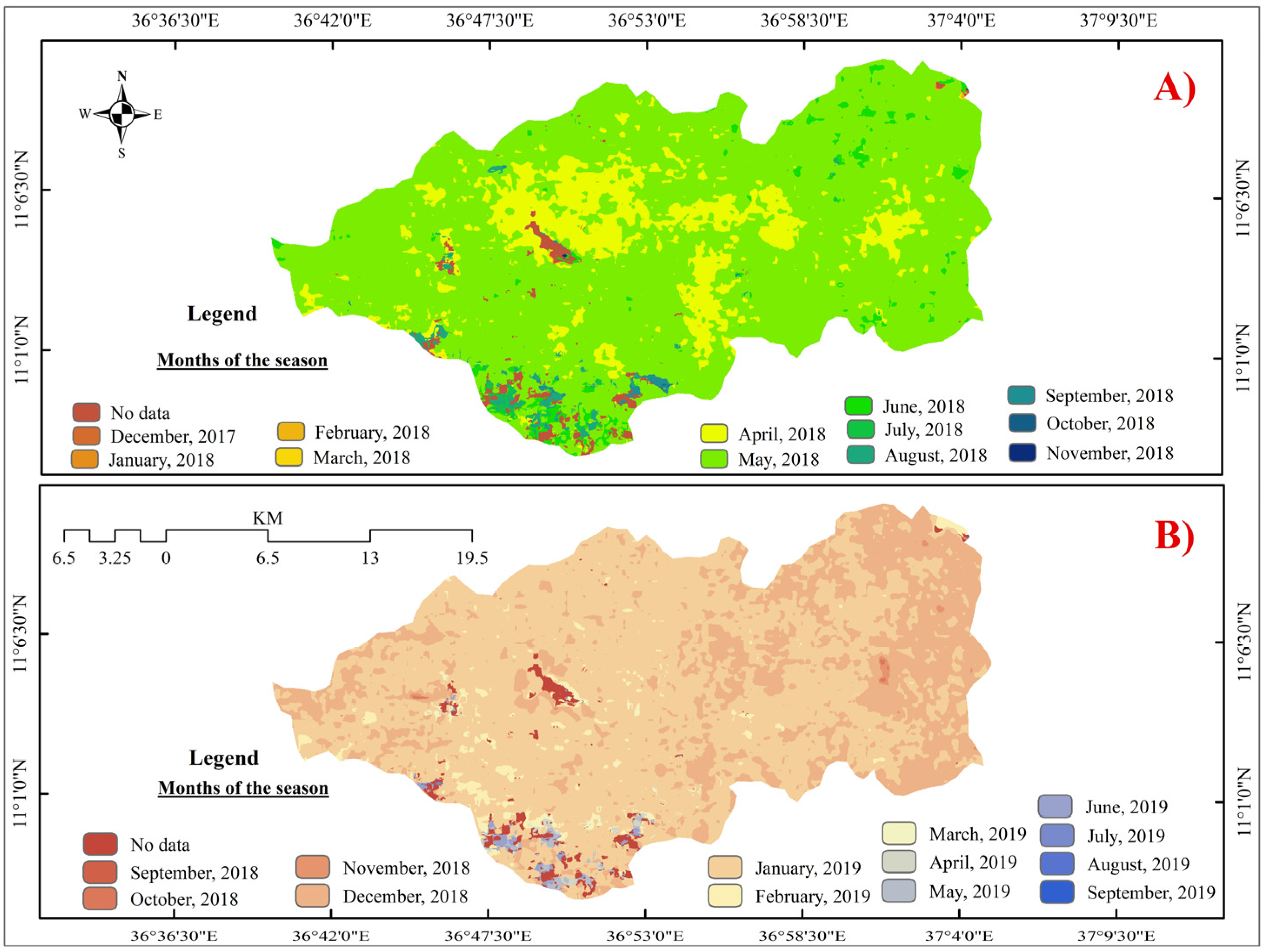
3.1. Seasonal Changes

Indicators of seasonal changes in the annual cycle of the NDVI were extracted for the identified vegetation types using TIMESAT. In vegetated areas with similar vegetation types and homogeneous compositions, monitoring indicators of seasonal change using satellite NDVI can prevent the effects of various ground-based observation noises [65]. For each vegetation type, the average value of all identified parameters was calculated from 2000 to 2020. The NDVI value of the study area showed an increase throughout the study period, with variation from season to season observed for most types of vegetation. In Figure 4, the sample pixel (latitude: 11.0453°N, longitude: 36.8631°E) representing an Acacia decurrens plantation in the central part of the study area shows the harmonic model fitted to the NDVI raw values and SG smoothed data across the study period. The trend decomposition of the NDVI shows that there was a remarkable increase, especially starting around 2010 (Figure 4).
Seasonal parameter values were extracted for the phenology indicators SOS, EOS, and LOS and the ecosystem condition indicators PV, BV, Amp, LI, and SI for distinct types of vegetation: natural forest, Acacia decurrens plantation forest, Eucalyptus plantation forest, grassland, and croplands. The results reveal specific variations in the patterns of the vegetation type responses across the study period. Cropland and plantation forests showed a relatively similar pattern for SOS and EOS. Grasslands showed slight variation throughout the study period for all phenological indicators. The earliest and latest growing events were recorded in natural forests, but the changes from year to year were relatively gradual (Figure 5A). Croplands were the first to be identified by EOS across the entire study period (Figure 5B).
The phenology indicator parameters are shown in Figure 6 using error bar plots, sorted based on the mean values from the largest number of days to fewest.
For most of the vegetation in the study area, the SOS occurs in April, May and June, while the EOS is observed from November to February (Figure 7).
The ecosystem status indicator parameters showed that the natural forest had the highest values of PV and BV and the lowest values of Amp and SI across the entire period (Figure 8). The patterns of Acacia decurrens and Eucalyptus plantation forests were relatively similar for most parameters. For example, the PV, BV, and LI of Acacia decurrens and Eucalyptus plantation forests increased during the study period, while the Amp and SI values decreased (Figure 8). The grassland pattern remained without noticeable variations in Amp and SI, similar to the phenology indicator parameters (Figure 8C,E).
The ecosystem condition indicator parameters are displayed in Figure 9 using error bar plots, sorted based on the mean values from the highest value to smallest.
The correlation values of SOS were below 0.2 for all vegetation types. EOS and LOS did not show significant changes for any vegetation type during the study period either. Acacia decurrens (0.97), Eucalyptus (0.95), and grassland (0.91) showed a higher correlation than the other vegetation types based on PV. Croplands and natural forests exhibited relatively low changes across the study seasons in terms of BV, Amp, and LI (Table 1).

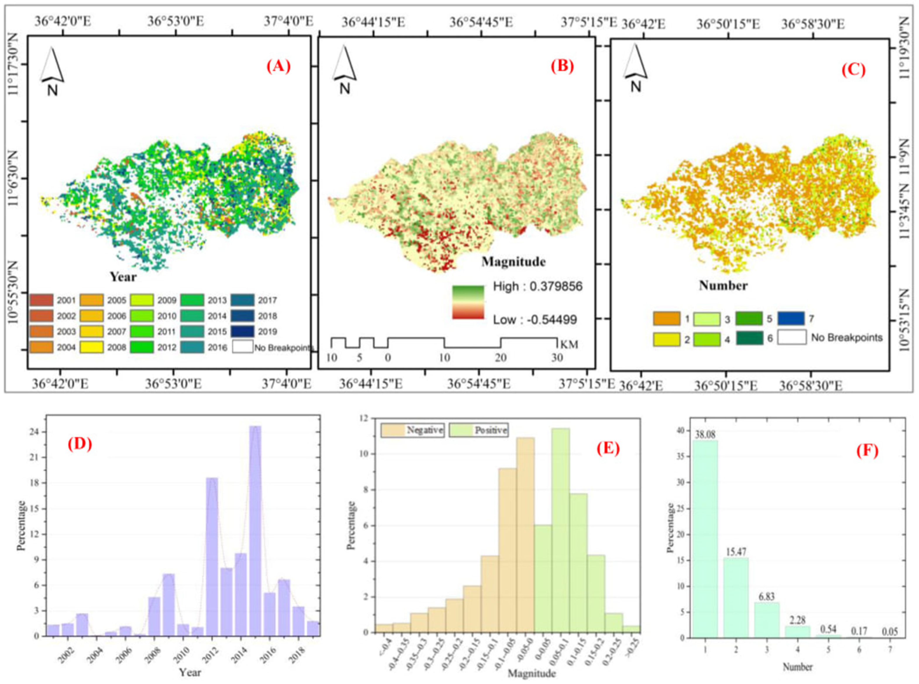
3.2. Interannual Changes

The BFAST algorithm was run for all NDVI pixels for the entire period to extract the year of the largest breakpoint, the magnitude of change for the largest breakpoint, and the number of breakpoints in each pixel. The magnitude and number of breakpoints in vegetation indicate the ecosystem condition and stability status, respectively. Most of the study areas (63.32% of the total) experienced breakpoints. The spatial distribution and area percentage of the largest breakpoints in all pixels for each year are shown in Figure 10A,D, respectively. The results show that the highest percentage of breakpoints occurred in 2015 (24.7%), 2012 (18.6%), and 2014 (9.8%). By contrast, the lowest percentage of breakpoints was observed in 2004 (0.1%), 2007 (0.2%), and 2005 (0.5%).
The magnitude and direction (positive changes or increasing NDVI trends and negative changes or decreasing NDVI trends) of the breakpoints for the time series data are shown in Figure 10B,E. The magnitude of the annual change varied from −0.54 to 0.38. The observed changes between −0.2 and 0.2 accounted for 93% of the area. The frequencies of magnitudes with values near zero were relatively high.
The number of largest breakpoints detected in the NDVI for each pixel varied from one to seven. Approximately 38.08% of the districts had one breakpoint, 15.47% had two breakpoints, 6.83% had three breakpoints, and 2.28% had four breakpoints. Areas with five, six, and seven breakpoints represented only 0.76% of the study area (Figure 10C,F).

4. Discussion

This study investigated the potential of using NDVI time series data to track and interpret local-level vegetation trends following plantation practices in the Northwestern Highlands of Ethiopia. The NDVI value of the study area exhibited a typical increase, which was characterized by seasonal and interannual vegetation changes. Our findings demonstrate that these changes can be exploited using satellite time series images to analyze vegetation trends and their implications for ecosystem conditions. These techniques can be used to monitor vegetation trends across decades, depending on the availability of satellite data and plantation types. The findings presented here hold promise for their use in identifying different parameter trajectories for vegetation types and their implications for ecosystem conditions. The ability of forest managers to assess ecosystem conditions following plantation practices can inform and optimize restoration strategies.

4.1. Seasonal Changes

The SG algorithm in TIMESAT revealed that the SOS for most vegetation in the study area was May and June. This is when most of the highlands of the country, including the study area, start receiving rainfall [35]. Throughout the study period, the order of growth initiation was as follows: grasslands followed by Eucalyptus plantation forests, croplands, and Acacia decurrens plantations. Grasslands begin to grow early and are relatively sensitive to weather conditions. Natural forests begin growing late, mostly in mid-June, and some of them did not show growth within the specified threshold, which may have been due to the maturity stage of vegetation (Figure 5A). This might be the reason that remotely sensed NDVI time series have difficulty detecting phenological changes in evergreen forests, because the NDVI tends to be saturated in areas with large amounts of biomass, such evergreen forests [54].
The average EOS for croplands and grasslands was December, which is the start of the winter (dry) season. Among the identified vegetation types, EOS starts early on croplands, and this is due to most of the crops in the study area being annual crops that are harvested mostly in the months of December and January. In contrast, January was the EOS time for Acacia decurrens and Eucalyptus plantations during the study period. Natural forests stopped growing around February, which is relatively late compared to other vegetation types. The eastern part of the study area began the EOS earlier (Figure 6B). Some natural forests in the southwestern part of the study area had an EOS that continued to the next season, extending the growing period for more than one natural year. Evergreen forests lack a distinct seasonal cycle in the NDVI [66]. The average LOS in the last two decades was highest for Eucalyptus plantations (8.85 months) followed by Acacia decurrens plantations, grasslands, natural forests, and croplands (8.65, 8.45, 8.29, and 7.56 months), respectively. Between the first half (2000–2009) and the second half (2010–2020) of the study period, there was a significant increase in LOS for Acacia decurrens and Eucalyptus plantations from 8.03 months to 9.27 months, and 8.85 to 9.36 months, respectively. The LOS in the first half for both plantations was relatively similar to that of grasslands and croplands, which implies that before the practice of plantations, the land was covered by grasslands and croplands (Appendix A Figure A1). This result complements the findings of previous studies conducted in the study area [34], which found that, before the establishment of plantation forests, the district was predominantly covered with croplands and grasslands. The LOS of natural forests showed a slight decrease between the two decades from 8.78 to 7.8 months. Unlike for the other vegetation types, for natural forests, a seasonal cycle takes a relatively prolonged time, which might be related to the maturity level of the forests and their year of establishment (Figure 5). Most vegetation types did not show significant differences in the values of phenology indicators before and after the plantation developed, and this result is in line with the findings of Sharma [67], which showed that there was no significant difference in phenology parameters between protected and unprotected areas.
As shown in Figure 8A,B, there was a marked increase in PV and BV starting around 2010 for the Acacia decurrens plantation, Eucalyptus plantation, and grasslands. However, the PV and BV of croplands and natural forests remained relatively stable, with almost the same values (Figure 8). On the other hand, the Amp and SI of both plantations declined due to a positive change in BV, which implies an increase in green vegetation. The SI of evergreen vegetation may be small even if the total productivity of the vegetation is high [68]. The LI showed a relatively higher increase in the second half of the study period for the Acacia decurrens and Eucalyptus plantations. A relatively slight increase was also observed in grasslands and croplands, and a slight decline was recorded in natural forests. The LI value of plantations in recent years has been increasing, and the SI value has decreased, indicating that the ecosystem is highly productive with dense evergreen vegetation [69]. The presence of a homogenous and young canopy with a fast-growing nature and high stand density indicates a higher biomass expansion [69].

4.1.1. Seasonal Parameter Value Distribution for Vegetation Types

The phenology indicators are shown in Figure 6, using error bar plots, which were sorted according to the mean values, from a larger number of days to fewer. The mean value of SOS was earliest in grasslands, and this proves that grasses were highly responsive to spring rains. In other ways, natural forests require a relatively long time to show growth following the change in season. The EOS of cropland appears earlier, and the EOS of natural forest appears the latest. The observed range of EOS was between 322 and 536. Eucalyptus plantation forests have the largest mean value, which indicates the quality of the species’ ability to continue growing, even in dry months, by extracting underground water using its deep roots. This can be attributed to the fact that the roots of Eucalyptus are long, can grow up to 20–30 feet, and extract more water from the deepest parts of the soil [70]. Cropland exhibited the lowest mean LOS value because the crops were harvested approximately five months after planting. The LOS range for all vegetation types was 8.96 and 24.57, both recorded for natural forests in the 14th and 3rd seasons of the time series, respectively.
Natural forests had the highest mean PV because dense forests in the study area are green almost all days of the year and have higher NDVI values. The mean PV value of the croplands was the lowest (Figure 9A), suggesting that the crops remained green for some months of the year and that after harvest, the area could be bare land. The order of vegetation types based on PV and BV was the same (Figure 9A,B), which shows the existence of a strong relationship between the parameters. PV and BV values were high, especially in the last few years of the study period, for most of the vegetation types. These parameters are best for distinguishing the productivity level of vegetation classes, where higher NDVI values correspond to vegetation in ecosystems under recovery [71]. Unlike the PV values, croplands and natural forests had the highest and lowest mean Amp, respectively (Figure 9C). Grasslands and natural forests had the narrowest and widest Amp ranges, with values between 0.365 and 0.389 and 0.103 and 0.351, respectively. A narrow Amp is characteristic of mature forests [72]. Generally, increasing trends in PV and BV and decreasing trends in Amp values were observed for most vegetation types. These results are consistent with the findings of Leeuwen [73], who assessed the vegetation condition in a restored forest at risk of wildfire.
Natural forests had the highest mean LI, followed by Eucalyptus and Acacia decurrens plantations (Figure 9D). In terms of the mean SI value, Acacia decurrens had the highest and natural forests had the lowest. The range of SI values for both plantations was relatively wider than that for other vegetation types, which shows the significant effect of plantation practices on NDVI values (Figure 9E). According to the ecosystem condition indicator parameters, the order of vegetation types is the same for PV, BV, and LI. Likewise, Amp and SI also had a relatively similar order of vegetation types. The Amp and SI of grasslands did not show significant differences, indicating consistency for most of the parameters.

4.1.2. Correlation between Seasons and Seasonality Parameters

For phenology indicators, the correlation coefficient of SOS was higher than that of EOS in natural forests, grasslands, and croplands. The EOS correlation was higher than that of SOS and LOS for the Acacia decurrens plantation. This might be because the greenness of the plantation forests in the study area was relatively less affected by the beginning of the rainfall.
The correlation of PV was higher than that of Amp for all vegetation types. Amp decreased for all vegetation types, which correlated with an increase in the minimum seasonal NDVI rather than a decrease in the maximum NDVI. A reduction in Amp is an indicator of improved vegetation growth [59]. The Acacia decurrens plantation has the highest correlation of Amp, followed by the Eucalyptus plantation and grassland. In contrast, the lowest growth rate was observed in natural forests. The PV was higher than the BV for all vegetation types, except for natural forests. Among the other indicators of ecosystem conditions, the correlation of LI was higher than that of SI in vegetation types. This indicates that there were differences in these two ecosystem condition indicators before and after the plantation was established because of the difference in aboveground primary productivity. Land-use activities, such as conservation measures, have significant positive effects on LI and SI values [67].

4.2. Interannual Changes Analysis

Breakpoints provide evidence of the statistical significance of variations in NDVI values. Thus, when a breakpoint emerges, it indicates a substantial shift in NDVI values that cannot be statistically attributed to preceding periodic or linear trends [74]. This may be related to disruptions in anthropogenic or environmental factors [75]. For instance, negative breakpoints correspond to periods associated with drought, flooding, and fire events [76]. Most of the breakpoints occurred during the early years of the study period and corresponded with natural forests and wetlands, which implies the existence of deforestation activities at the time and the drying out of water-logged areas. The percentage of wetland cover in the area also shrank from 18.58% in 1973 to 0.2% in 2015 [34]. During the first half of the study period, the forest cover in the study area decreased, mainly due to population growth and related effects, such as increased demand for arable land, fuelwood, and construction wood [35]. The magnitude map (Figure 10B) also confirms that the southern parts of the study area, where natural forests are found, exhibited relatively extreme negative values. The largest area percentage of breakpoints was detected during 2015, and this value agrees with the TIMESAT result. The highest abrupt change in vegetation during 2015 caused a decrease in LI in plantations in 2016 (Figure 8D), which was highly correlated with plantation activities. Plantation practices may result in the detection of two breakpoints from a single pixel: during the greening period and after harvest. The effect seen in 2015 (BFAST) and 2016 (TIMESAT) might have been due to the harvest of more plantations for charcoal production. Farmers usually harvest plantations after four years and above to generate income [77].
Alternatively, positive peaks in the breakpoints are related to the practices of afforestation, ecological restoration, and policy-driven land-use conversions [75]. The breakpoints that happened in the second half of the study period were more intense, and this attributed to the expansion of plantation forests in the area. The results are consistent with the findings of Wondie and Mekuria [35], who demonstrated that the forest cover of Fagita Lekoma District increased by 5.2% between 2010 and 2015, from 11,397 ha to 17,330 ha. The area coverage of Acacia decurrens plantations has progressively increased since 2006 in the Guder watershed, which is one of the watersheds found in the district. The study by Birhan et al. [78] in the same watershed showed that between 2006 and 2017, a remarkable amount of land use/land cover was converted to plantation forests from cropland and grazing land, so the forest cover of the watershed increased by more than 400%. The forest cover of Fagita Lekoma District expanded by 1.2% per year between 1995 and 2015, mainly due to the planting of Acacia decurrens at the expense of cultivated land, which decreased by 1% per year [35]. The soil in Fagita Lekoma District is highly acidic [45], which is attributed to heavy rain and results in low crop productivity. This was one of the main driving factors that promoted the expansion of Acacia decurrens plantations in the district over the past few decades because this species has a leguminous character, which enables it to reduce soil acidity [79].
The spatial distribution of breakpoints that occurred in the natural forest during the early years of the study period shifted to other types of vegetation in the later years in various parts of the study area (Figure 10A). The findings of Belayneh et al. [37] also confirmed that the expansion of Acacia decurrens plantation forests in the study area reduced human and livestock pressure on natural forests by prioritizing firewood and reducing free grazing. Acacia decurrens plantation forest cover progressively increased across the district by 16% between 2000 and 2017 [38]. These changes in land use have enhanced vegetation regeneration and significantly altered the dynamics of vegetation status in the area. This might be related to the potential of Acacia decurrens in terms of soil erosion reduction and the recovery of soil fertility [79]. Moreover, Acacia decurrens serves a dual purpose by alleviating pressure on the natural forest, which has been suffering from a high rate of forest degradation due to the collection of fuelwoods and the production of charcoal, and by serving as an alternative land use that is more economically lucrative [80].
In the study area, apart from protected natural forests and some irrigated croplands, most of the land experienced at least one abrupt change in the NDVI between 2000 and 2020. The number of breakpoints was mostly linked to the establishment and harvesting of Acacia decurrens plantations. The spatial distribution map of the number of changes detected in the NDVI is shown in Figure 10C, where more than half of the district (53.55%) had one or two breakpoints. Most of the areas with frequent breakpoints were unevenly distributed in various parts of the study area and characterized by the early adoption of Acacia decurrens plantations.

4.3. Implications for the Ecosystem Condition

Fagita Lekoma District has degraded soils due to its large population density and higher rainfall distribution [81], in addition to continuous cultivation of the land for longer periods [43], as well as extensive deforestation that resulted in acidic soils of low fertility [82]. Programs implemented by the local and national government focused on the regeneration of the ecosystem may have produced a positive change in the condition of the vegetation [75]. The Acacia decurrens plantation has been promoted by both government and nongovernmental organizations because this species thrives on degraded lands, including gullies.
The trend component of the NDVI in the study area increased from year to year during the study period (Figure 11). The mean NDVI of the entire study area at the beginning and in the final years of the study period differed, which confirms how the high vegetation cover of the district has expanded. The five-years mean NDVI, which was 0.58 for the years 2000–2004, rose to 0.65 during 2015 and 2020. Such a positive change in the NDVI has shown implications for the productivity of the land and indicates the existence of changes in the overall ecological pattern [83]. A study by Mola and Linger [84] reported that there has been an improvement in soil fertility on land parcels covered by Acacia decurrens plantation forests. These results are consistent with another study conducted in the study area that also confirms that the expansion of Acacia decurrens plantations has affected the soil’s physical and chemical properties. For instance, the total nitrogen of the soil under Acacia decurrens plantations is 43.5% higher than that under cropland [78]. Likewise, the pH value of the soil under an Acacia decurrens plantation is 2% lower than the soil under cropland, whereas the availability of phosphorus in Acacia decurrens plantation soil is 1.25 mg kg−1 lower than that in cropland soil [78]. The degraded soils of the district have been considerably improved, mainly through the planting of Acacia decurrens and enhanced natural capital [82], and the ecosystem service value increased by 54% from 2006 to 2017 [36]. Acacia decurrens plantations are typical biological measures for the restoration of highly degraded land and improving resilience to climate shocks [85].
The TIMESAT results for ecosystem condition indicators (Figure 8) show that there was a significant change in most parameters within the identified study period. For example, the PV, BV, and LI increased, especially for Acacia decurrens plantations, Eucalyptus plantations, and grassland. These indicators account for the most substantial variations and exhibit strong correlations with the presence of vegetation cover [86].
The Amp and SI for most of the vegetation types were characterized by negative changes due to the increase in the BV, which is an indicator of stable vegetation condition and the restoration of the ecosystem. Lower values of SI and higher values of LI imply that the vegetation under consideration is a highly productive ecosystem with dense canopy cover [69]. The growth of the relative amount of vegetation biomass is an indicator of gradual ecosystem restoration [41].
The BFAST results also confirm that there was a change in the ecosystem in terms of the magnitude and number of breakpoints during the study period. The study area exhibited breakpoints for the identified years at different percentages (Figure 10A,D). Changes at the beginning of the study period were mostly characterized by a negative magnitude. Before the start of the plantation practice, the forest cover was diminishing in the district [78] due to population growth and related effects, such as increased demand for arable land, fuelwood, and construction wood [35]. However, around 2010, positive changes dominated, and around half of the area with abrupt changes was characterized by positive changes. This finding is in line with that of Wondie and Mekuria [35], who reported that forest cover has increased since 2010 because of the expansion of Acacia decurrens plantations. The forest cover of the district has shown an upward trend over the last two decades because of Acacia decurrens plantations and the regeneration of previously degraded natural forests because of a reduction in the normal pressure on natural forests achieved through the replacement of fuelwood and construction materials [37]. The expansion of Acacia decurrens plantation forest plays a vital role in biophysical environment rehabilitation and conservation [38]. As a result, more than 30% of the study area exhibited a positive breakpoint magnitude during the study period, and approximately 36% remained without abrupt changes. The negative changes experienced in recent years are related to the harvesting of plantations that the community replants immediately after.
In general, the analysis in this study shows that seasonal and interannual changes enable the inference of changes in the ecosystem. Both the TIMESAT and BFAST outputs, along with the increasing trend of the average NDVI, indicate significant vegetation regeneration, serving as significant indicators of ecosystem restoration.

5. Conclusions

Changes in seasonal and interannual vegetation trends play a significant role in determining the condition of an ecosystem. Plantation-mediated shifts in seasonal and interannual vegetation changes underscore the importance of identifying parameters and methods for analyzing ecosystem conditions. In line with our objectives, we conducted a study in the Northwestern Highlands of Ethiopia focused on utilizing NDVI time series data to monitor and interpret local-level vegetation trends, especially following plantation practices. The findings and implications of this research provide valuable insights into the dynamics of vegetation and ecosystem conditions in the area.
The spatiotemporal behavior of most types of vegetation showed that in the study area, vegetation changes in the last two decades have had a more pronounced effect on ecosystem condition indicators than on phenology indicators. Breakpoints in NDVI data highlighted significant shifts in vegetation cover. Negative breakpoints during the early years of the study period were associated with deforestation. Most of the largest breakpoints were detected during the second half of the study period and were linked to afforestation and land-use conversions, primarily due to the expansion of Acacia decurrens plantation practices. Positive changes in NDVI trends suggest an improvement in ecosystem condition, particularly in vegetation cover and productivity. The findings of applied data decomposition algorithms have significant implications for ecosystem restoration and conservation efforts in the study area. The promotion of plantation practices, particularly Acacia decurrens, has positively impacted vegetation regeneration, contributing to improved ecosystem health.
Overall, the study demonstrates that the adoption of afforestation practices, such as the cultivation of Acacia decurrens plantation forests, has led to positive changes in ecosystem conditions in Fagita Lekoma District. These findings provide valuable guidance for land-use planning, conservation, and sustainable ecosystem management in regions facing challenges like soil degradation and deforestation. The study highlights the potential of leveraging remote sensing data to monitor and manage ecosystems effectively over time, contributing to ecological resilience and improved environmental conditions in the study area.

Author Contributions

Conceptualization, B.A., J.S.-M. and J.R.; methodology, B.A., J.S.-M. and J.R.; software, B.A., J.S.-M. and S.A.K.; validation, B.A. and J.S.-M.; formal analysis, B.A.; investigation, B.A. and J.S.-M.; resources, B.A. and J.S.-M.; data curation; B.A. and S.A.K.; writing—original draft preparation, B.A.; writing—review and editing, B.A. and J.S.-M.; visualization, B.A.; supervision, J.S.-M. and J.R. All authors have read and agreed to the published version of the manuscript.

Funding

This research received no external funding.

Data Availability Statement

The data from the current study are available from corresponding author upon request.

Conflicts of Interest

The authors declare no conflict of interest.

Appendix A

Figure A1. NDVI data decomposed results using TIMESAT for the identified vegetation types in the study area: (A) Eucalyptus plantation forest, (B) natural forest, (C) grassland, and (D) cropland.
Remotesensing 15 05032 g0a1
Figure A2. Vegetation types considered for TIMESAT in the study area (Google Earth image).
Remotesensing 15 05032 g0a2
Table A1. Definition of seasonal parameters.
Phenology IndicatorsEcosystem Condition Indicators
1.
SOS: time for which the left edge has increased to 25% seasonal amplitude as measured from the left minima of the curve.
1.
PV: maximum NDVI value for the fitted function during the season.
2.
BV: average between left and right minima curve. NDVI value during dormancy.
2.
EOS: time for which the right edge has decreased to 25% seasonal amplitude from the right minima of the curve.
3.
Amp: the difference between PV and BV.
4.
LI: integral of the fitted function describing the season and the zero level from the SOS to EOS.
3.
LOS: time from the SOS to EOS.
5.
SI: integral of the difference between the fitted function describing the season and the BV from the SOS to EOS. Vegetation production between dormancy and peak growth.
Table A2. NDVI time series data processing input setting in TIMESAT used for this study.
ParameterValueDescription
Spike method1Spike method: 0 = no spike filtering, 1 = method based on median filtering, 2 = weights from STL, 3 = weights from STL multiplied with original weights.
Spike value2Determines the degree of removal and a low value will remove more spikes.
STL stiffness value2STL trend stiffness parameter. Its value is between 1 and 10 with a default of 3.
Seasonal parameter1A value close to 0 will attempt to fit two seasons per year and a value near 1 attempt to fit one season.
Number of envelope iterations1Number of iterations for upper envelope adaptation (3,2,1).
Adaptation strength2Envelope adaptation strength. The maximum strength is 10.
SG window size4The half window for SG filtering. Large values will give a high degree of smoothing.
Start/end of season1Season start method for determining the start/end of the season based on the intersection of the fitted curve: 1 = Seasonal amplitude, at the point where the curve intersects a proportion of the seasonal amplitude; 2 = absolute value, at the point where the curve intersects an absolute value in units of the data; 3 = relative amplitude, at the point where the curve intersects a proportion of a relative seasonal amplitude; 4 = STL trend, at the intersection with the trend line from STL.
Season start/end0.25Values for determining season start/end. If the start method is 1 or 3, the value must be between 0 and 1.

References

  1. Cai, B.; Yu, R. Advance and evaluation in the long time series vegetation trends research based on remote sensing. J. Remote Sens. 2009, 4619, 1170–1186. [Google Scholar]
  2. Wei, F.; Wang, S.; Fu, B.; Pan, N.; Feng, X.; Zhao, W.; Wang, C. Vegetation dynamic trends and the main drivers detected using the ensemble empirical mode decomposition method in East Africa. Land. Degrad. Dev. 2018, 29, 2542–2553. [Google Scholar] [CrossRef]
  3. Wang, X.; Piao, S.; Ciais, P.; Li, J.; Friedlingstein, P.; Koven, C.; Chen, A. Spring temperature change and its implication in the change of vegetation growth in North America from 1982 to 2006. Proc. Natl. Acad. Sci. USA 2011, 108, 1240–1245. [Google Scholar] [CrossRef]
  4. Ohana-Levi, N.; Paz-Kagan, T.; Panov, N.; Peeters, A.; Tsoar, A.; Karnieli, A. Time series analysis of vegetation-cover response to environmental factors and residential development in a dryland region. GIsci Remote Sens. 2019, 56, 362–387. [Google Scholar] [CrossRef]
  5. De Jong, R.; De Bruin, S. Linear trends in seasonal vegetation time series and the modifiable temporal unit problem. Biogeosciences 2012, 9, 71–77. [Google Scholar] [CrossRef]
  6. Brandon, T.; Ellison, A.M.; Fraser, W.R.; Gorman, K.B.; Holbrook, S.J.; Laney, C.M.; Ohman, M.D.; Peters, D.P.C.; Pillsbury, F.C.; Rassweiler, A.; et al. Analysis of Abrupt Transitions in Ecological Systems; Harvard University: Cambridge, MA, USA, 2011. [Google Scholar] [CrossRef]
  7. Browning, D.M.; Maynard, J.J.; Karl, J.W.; Peters, D.C. Breaks in MODIS time series portend vegetation change: Verification using long-term data in an arid grassland ecosystem: Verification. Ecol. Appl. 2017, 27, 1677–1693. [Google Scholar] [CrossRef]
  8. Mondal, S.; Jeganathan, C.; Amarnath, G.; Pani, P. Time-series cloud noise mapping and reduction algorithm for improved vegetation and drought monitoring. GIsci Remote Sens. 2017, 54, 202–229. [Google Scholar] [CrossRef]
  9. Guan, X.; Huang, C.; Zhang, R. Article integrating modis and landsat data for land cover classification by multilevel decision rule. Land 2021, 10, 208. [Google Scholar] [CrossRef]
  10. Cohen, W.B.; Goward, S.N. Landsat’s role in ecological applications of remote sensing. Bioscience 2004, 54, 535–545. [Google Scholar] [CrossRef]
  11. Yang, D.; Su, H.; Yong, Y. MODIS-Landsat Data Fusion for Estimating Vegetation Dynamics—A Case Study for Two Ranches in Southwestern Texas; Conference Proceedings Paper—Remote Sensing. In Proceedings of the 1st International Electronic Conference on Remote Sensing, Online, 22 June–5 July 2015; p. d016. [Google Scholar] [CrossRef]
  12. Justice, C.O.; Vermote, E.; Townshend, J.R.G.; Defries, R.; Roy, D.P. The moderate resolution imaging spectroradiometer (MODIS): Land remote sensing for global change research. IEEE Trans. Geosci. Remote Sens. 1998, 36, 1228–1249. [Google Scholar] [CrossRef]
  13. Hilker, T.; Anderson, M.C.; Masek, J.G.; Wang, P. Fusing Landsat and MODIS Data for Vegetation Monitoring. IEEE Geosci. Remote Sens. Mag. 2015, 3, 47–60. [Google Scholar]
  14. Camps-Valls, G.; Tuia, D.; Bruzzone, L.; Benediktsson, J.A. Advances in hyperspectral image classification: Earth monitoring with statistical learning methods. IEEE Signal Process Mag. 2014, 31, 45–54. [Google Scholar] [CrossRef]
  15. Zhu, Z. Change detection using landsat time series: A review of frequencies, preprocessing, algorithms, and applications. ISPRS J. Photogramm. Remote Sens. 2017, 130, 370–384. [Google Scholar] [CrossRef]
  16. Omuto, C.T. A new approach for using time-series remote-sensing images to detect changes in vegetation cover and composition in drylands: A case study of eastern Kenya. Int. J. Remote Sens. 2011, 32, 6025–6045. [Google Scholar] [CrossRef]
  17. Ramachandra, T.V.; Kumar, U.; Dasgupta, A. Analysis of Land Surface Temperature and Rainfall with Landscape Dynamics in Western Ghats, India; Indian Institute of Science: Bangalore, India, 2016. [Google Scholar]
  18. Eklundh, L.; Jöhnsson, P. TIMESAT 3.3 Software Manual. 2017, pp. 1–92. Available online: https://web.nateko.lu.se/timesat/docs/TIMESAT33_SoftwareManual.pdf (accessed on 25 March 2022).
  19. Rodrigues, A.S. Analysis of Vegetation Dynamics Using Time-Series Vegetation Index Data from Earth Observation Satellites. Ph.D. Thesis, University of Porto, Porto, Portugal, 2014; pp. 1–156. [Google Scholar]
  20. Verbesselt, J.; Zeileis, A.; Herold, M. Near real-time disturbance detection using satellite image time series. Remote Sens. Environ. 2012, 123, 98–108. [Google Scholar] [CrossRef]
  21. Colditz, R.R.; Gessner, U.; Conrad, C.; van Zyl, D.; van Zyl, D.; Malherbe, J.; Landmann, T.; Schmidt, M.; Dech, S. Dynamics of MODIS time series for ecological applications in Southern Africa. In Proceedings of the MultiTemp 2007–2007 International Workshop on the Analysis of Multi-Temporal Remote Sensing Images, Leuven, Belgium, 18–20 July 2007. [Google Scholar] [CrossRef]
  22. De Beurs, K.M.; Henebry, G.M. Spatio-temporal statistical methods for modelling land surface phenology. In Phenological Research: Methods for Environmental and Climate Change Analysis; Springer: Berlin/Heidelberg, Germany, 2010; pp. 177–208. [Google Scholar] [CrossRef]
  23. Zeng, L.; Wardlow, B.D.; Xiang, D.; Hu, S.; Li, D. A review of vegetation phenological metrics extraction using time-series, multispectral satellite data. Remote Sens. Environ. 2020, 237, 111511. [Google Scholar] [CrossRef]
  24. Shen, M.; Tang, Y.; Chen, J.; Zhu, X.; Zheng, Y. Influences of temperature and precipitation before the growing season on spring phenology in grasslands of the central and eastern Qinghai-Tibetan Plateau. Agric. For. Meteorol. 2011, 151, 1711–1722. [Google Scholar] [CrossRef]
  25. Chen, X.; Wang, W.; Chen, J.; Zhu, X.; Shen, M.; Gan, L.; Gao, X. Does any phenological event defined by remote sensing deserve particular attention? An examination of spring phenology of winter wheat in Northern China. Ecol. Indic. 2020, 116, 106456. [Google Scholar] [CrossRef]
  26. Palareti, G.; Legnani, C.; Cosmi, B.; Antonucci, E.; Erba, N.; Poli, D.; Testa, S.; Tosetto, A. Comparison between different D-Dimer cutoff values to assess the individual risk of recurrent venous thromboembolism: Analysis of results obtained in the DULCIS study. Int. J. Lab. Hematol. 2016, 38, 42–49. [Google Scholar] [CrossRef]
  27. Djebou, D.C.S.; Singh, V.P.; Frauenfeld, O.W. Vegetation response to precipitation across the aridity gradient of the southwestern United states. J. Arid. Environ. 2015, 115, 35–43. [Google Scholar] [CrossRef]
  28. Nigussie, Z.; Tsunekawa, A.; Haregeweyn, N.; Adgo, E.; Tsubo, M.; Ayalew, Z.; Abele, S. Economic and financial sustainability of an Acacia decurrens-based Taungya system for farmers in the Upper Blue Nile Basin, Ethiopia. Land Use Policy 2020, 90, 104331. [Google Scholar] [CrossRef]
  29. Garrity, D.P. Agroforestry and the achievement of the Millennium Development Goals. Agrofor. Syst. 2004, 61, 5–17. [Google Scholar]
  30. Negelle, A.; Central, S. Expansion of Eucalypt Farm Forestry and Its Determinants in Arsi Negelle District, South Central Ethiopia. Small-Scale For. 2012, 11, 389–405. [Google Scholar] [CrossRef]
  31. Bazie, Z.; Feyssa, S.; Amare, T. Effects of Acacia decurrens Willd. tree-based farming system on soil quality in Guder watershed, North Western highlands of Ethiopia. Cogent Food Agric. 2020, 6, 1743622. [Google Scholar] [CrossRef]
  32. Orchard, S.; Smith, E. Managing the Environmental Effects of Plantation Forestry: A Case Study in the Ngunguru Catchment, Northland, New Zealand. 2013. Available online: https://www.researchgate.net/publication/298679188_Managing_the_environmental_effects_of_plantation_forestry_a_case_study_in_the_Ngunguru_catchment_Northland_New_Zealan (accessed on 4 July 2022).
  33. Inge, I.; Walle, V. Carbon Sequestration in Short-Rotation Forestry Plantations and in Belgian Forest Ecosystems. Ph.D. Thesis, Ghent University, Ghent, Belgium, 2007; pp. 1–244. [Google Scholar]
  34. Alemayehu, B. GIS and Remote Sensing Based Land Use/Land Cover Change Detection and Prediction in Fagita Lekoma Woreda, Awi Zone, Northwestern Ethiopia. Master’s Thesis, Addis Ababa University, Addis Ababa, Ethiopia, 2015; pp. 1–85. [Google Scholar]
  35. Wondie, M.; Mekuria, W. Planting of acacia decurrens and dynamics of land cover change in fagita lekoma district in the Northwestern Highlands of Ethiopia. Mt. Res. Dev. 2018, 38, 230–239. [Google Scholar] [CrossRef]
  36. Berihun, M.L.; Tsunekawa, A.; Haregeweyn, N.; Tsubo, M.; Fenta, A.A. Changes in ecosystem service values strongly influenced by human activities in contrasting agro-ecological environments. Ecol. Process 2021, 10, 1–18. [Google Scholar] [CrossRef]
  37. Belayneh, Y.; Ru, G.; Guadie, A.; Teffera, Z.L. Forest cover change and its driving forces in Fagita Lekoma. J. For. Res. 2020, 31, 1567–1582. [Google Scholar] [CrossRef]
  38. Worku, T.; Mekonnen, M.; Yitaferu, B.; Cerdà, A. Conversion of crop land use to plantation land use, northwest Ethiopia. Trees For. People 2021, 3, 100044. [Google Scholar] [CrossRef]
  39. Abbes, A.B.; Bounouh, O.; Farah, I.R.; de Jong, R.; Martínez, B. Comparative study of three satellite image time-series decomposition methods for vegetation change detection. Eur. J. Remote Sens. 2018, 51, 607–615. [Google Scholar] [CrossRef]
  40. Bonannella, C.; Chirici, G.; Travaglini, D.; Pecchi, M.; Vangi, E.; D’Amico, G.; Giannetti, F. Characterization of Wildfires and Harvesting Forest Disturbances and Recovery Using Landsat Time Series: A Case Study in Mediterranean Forests in Central Italy. Fire 2022, 5, 68. [Google Scholar] [CrossRef]
  41. Ma, J.; Zhang, C.; Guo, H.; Chen, W.; Yun, W.; Gao, L.; Wang, H. Analyzing ecological vulnerability and vegetation phenology response using NDVI time series data and the BFAST algorithm. Remote Sens. 2020, 12, 3371. [Google Scholar] [CrossRef]
  42. Chirici, G.; Giannetti, F.; Mazza, E.; Francini, S.; Travaglini, D.; Pegna, R. Monitoring clearcutting and subsequent rapid recovery in Mediterranean coppice forests with Landsat time series. Ann. For. Sci. 2020, 77, 40. [Google Scholar] [CrossRef]
  43. Yibeltal, M.; Tsunekawa, A.; Haregeweyn, N.; Adgo, E.; Meshesha, D.T.; Aklog, D.; Masunaga, T.; Tsubo, M.; Billi, P.; Vanmaercke, M.; et al. Analysis of long-term gully dynamics in different agro-ecology settings. Catena 2019, 179, 160–174. [Google Scholar] [CrossRef]
  44. Alemu, G.T.; Tsunekawa, A.; Haregeweyn, N.; Nigussie, Z.; Tsubo, M.; Elias, A.; Ayalew, Z.; Berihun, D.; Adgo, E.; Meshesha, D.T.; et al. Smallholder farmers’ willingness to pay for sustainable land management practices in the Upper Blue Nile basin, Ethiopia. Environ. Dev. Sustain. 2021, 23, 5640–5665. [Google Scholar] [CrossRef]
  45. Ebabu, K.; Atsushi, T.; Nigussie, H.; Enyew, A.; Tsegaye, M.D.; Dagnachew, A.; Tsugiyuki, M.; Mitsuru, T.; Dagnenet, S.; Almaw, F.A.; et al. Analyzing the variability of sediment yield: A case study from paired watersheds in the Upper Blue Nile basin, Ethiopia. Geomorphology 2018, 303, 446–455. [Google Scholar] [CrossRef]
  46. Maynard, J.J.; Karl, J.W.; Browning, D.M. Effect of spatial image support in detecting long-term vegetation change from satellite time-series. Landsc. Ecol. 2016, 31, 2045–2062. [Google Scholar] [CrossRef]
  47. Viña, A.; Liu, W.; Zhou, S.; Huang, J.; Liu, J. Land surface phenology as an indicator of biodiversity patterns. Ecol. Indic. 2016, 64, 281–288. [Google Scholar] [CrossRef]
  48. Teferi, E.; Uhlenbrook, S.; Bewket, W. Inter-annual and seasonal trends of vegetation condition in the Upper Blue Nile (Abay) Basin: Dual-scale time series analysis. Earth Syst. Dyn. 2015, 6, 617–636. [Google Scholar] [CrossRef]
  49. Eklundh, L.; Per, J. Chapter 7 TIMESAT: A Software Package for Time-Series Processing and Assessment of Vegetation Dynamics. In Remote Sensing Time Series; Springer: Berlin/Heidelberg, Germany, 2015. [Google Scholar] [CrossRef]
  50. Huete, A.R. Modis Vegetation Index Algorithm Theoretical Basis v3. 1999. Available online: https://modis.gsfc.nasa.gov/data/atbd/atbd_mod13.pdf (accessed on 17 January 2022).
  51. Jamali, S.; Jönsson, P.; Eklundh, L.; Ardö, J.; Seaquist, J. Detecting changes in vegetation trends using time series segmentation. Remote Sens. Environ. 2015, 156, 182–195. [Google Scholar] [CrossRef]
  52. Gross, D. Monitoring Agricultural Biomass Using NDVI Time Series; Food and Agriculture Organization of the United Nations (FAO): Rome, Italy, 2005; pp. 1–17. [Google Scholar]
  53. Tomov, H.D. Automated Temporal NDVI Analysis over the Middle East for the Period. Master’s Thesis, Lund University, Lund, Sweden, 2016; pp. 1–129. [Google Scholar]
  54. Huete, A.; Didan, K.; Miura, T.; Rodriguez, E.P.; Gao, X.; Ferreira, L.G. Overview of the Radiometric and Biophysical Performance of the MODIS Vegetation Indices. 2002. Available online: www.elsevier.com/locate/rse (accessed on 23 March 2022).
  55. Jönsson, P.; Eklundh, L. TIMESAT—A program for analyzing time-series of satellite sensor data. Comput. Geosci. 2004, 30, 833–845. [Google Scholar] [CrossRef]
  56. Stanimirova, R.; Cai, Z.; Melaas, E.K.; Gray, J.M.; Lars, E.; Per, J.; Friedl, M.A. An empirical assessment of the MODIS land cover dynamics and TIMESAT land surface phenology algorithms. Remote Sens. 2019, 11, 2201. [Google Scholar] [CrossRef]
  57. Cai, Y.; Liu, S.; Lin, H. Monitoring the vegetation dynamics in the dongting lake wetland from 2000 to 2019 using the BEAST algorithm based on dense landsat time series. Appl. Sci. 2020, 10, 4209. [Google Scholar] [CrossRef]
  58. Li, Y.; Qin, Y.; Ma, L.; Pan, Z. Climate change: Vegetation and phenological phase dynamics. Int. J. Clim. Chang. Strateg. Manag. 2020, 12, 495–509. [Google Scholar] [CrossRef]
  59. Heumann, B.W.; Seaquist, J.W.; Eklundh, L.; Jönsson, P. AVHRR derived phenological change in the Sahel and Soudan, Africa, 1982–2005. Remote Sens. Environ. 2007, 108, 385–392. [Google Scholar] [CrossRef]
  60. Pockrandt, B.R. A Multi-Year Comparison of Vegetation Phenology Between Military Training Lands and Native Tallgrass Prairie Using TIMESAT and Moderate-Resolution Satellite Imagery. Implement. Sci. 2012, 39, 1–24. Available online: https://krex.k-state.edu/bitstream/handle/2097/17320/BryannaPockrandt2014.pdf?sequence=1&isAllowed=y (accessed on 15 February 2022).
  61. Lebrini, Y.; Boudhar, A.; Htitiou, A.; Hadria, R.; Lionboui, H.; Bounoua, L.; Benabdelouahab, T. Remote monitoring of agricultural systems using NDVI time series and machine learning methods: A tool for an adaptive agricultural policy. Arab. J. Geosci. 2020, 13, 796. [Google Scholar] [CrossRef]
  62. Verbesselt, J.; Hyndman, R.; Newnham, G.; Culvenor, D. Detecting trend and seasonal changes in satellite image time series. Remote Sens. Environ. 2010, 114, 106–115. [Google Scholar] [CrossRef]
  63. Khan, S.A.; Vanselow, K.A.; Sass, O.; Samimi, C. Detecting abrupt change in land cover in the eastern Hindu Kush region using Landsat time series (1988–2020). J. Mt. Sci. 2022, 19, 1699–1716. [Google Scholar] [CrossRef]
  64. Watts, L.M.; Laffan, S.W. Effectiveness of the BFAST algorithm for detecting vegetation response patterns in a semi-arid region. Remote Sens. Environ. 2014, 154, 234–245. [Google Scholar] [CrossRef]
  65. Zhou, Y.Z.; Jia, G.S. Precipitation as a control of vegetation phenology for temperate steppes in China. Atmos. Ocean. Sci. Lett. 2016, 9, 162–168. [Google Scholar] [CrossRef]
  66. Shi, S.; Yang, P.; van der Tol, C. Spatial-temporal dynamics of land surface phenology over Africa for the period of 1982–2015. Heliyon 2023, 9, e16413. [Google Scholar] [CrossRef]
  67. Sharma, G. Land Surface Phenology as an Indicator of Conservation Policies like Natura2000; Lund: Göteborg, Sweden, 2016. [Google Scholar]
  68. Chamberlain, D.A.; Phinn, S.R.; Possingham, H.P. Mangrove Forest cover and phenology with landsat dense time series in central queensland, australia. Remote Sens. 2021, 13, 3032. [Google Scholar] [CrossRef]
  69. Deka, J.; Kalita, S.; Khan, M.L. Vegetation Phenological Characterization of Alluvial Plain Shorea robusta-dominated Tropical Moist Deciduous Forest of Northeast India Using MODIS NDVI Time Series Data. J. Indian. Soc. Remote Sens. 2019, 47, 1287–1293. [Google Scholar] [CrossRef]
  70. Hayet, S.; Sujan, K.M.; Mustari, A.; Miah, M.A. Hemato-biochemical profile of turkey birds selected from Sherpur district of Bangladesh. Int. J. Adv. Res. Biol. Sci. 2021, 8, 1–5. [Google Scholar] [CrossRef]
  71. Martínez, J.J.R.; Gao, Y. Forest Disturbance Analysis by Phenology of Forest Covers in Mexico Using Time Series NDVI Data for the Period of 2014–2016. 2020. Available online: http://www.inegi.org.mx/geo/contenidos/recnat/usosuelo/ (accessed on 11 August 2023).
  72. Walker, J.J.; Soulard, C.E. Phenology patterns indicate recovery trajectories of ponderosa pine forests after high-severity fires. Remote Sens. 2019, 11, 2782. [Google Scholar] [CrossRef]
  73. Van Leeuwen, W.J.D. Monitoring the Effects of Forest Restoration Treatments on Post-Fire Vegetation Recovery with MODIS Multitemporal Data. Sensors 2008, 8, 2017–2042. [Google Scholar] [CrossRef]
  74. Nghiem, J.; Potter, C.; Baiman, R. Detection of vegetation cover change in renewable energy development zones of southern California using MODIS NDVI time series analysis, 2000 to 2018. Environments 2019, 6, 40. [Google Scholar] [CrossRef]
  75. Geng, L.; Che, T.; Wang, X. Detecting Spatiotemporal Changes in Vegetation with the BFAST Model in the Qilian Mountain Region during 2000–2017. Remote Sens. 2019, 11, 103. [Google Scholar] [CrossRef]
  76. Chen, L.; Michishita, R.; Xu, B. ISPRS Journal of Photogrammetry and Remote Sensing Abrupt spatiotemporal land and water changes and their potential drivers in Poyang Lake, 2000–2012. Isprs J. Photogramm. Remote Sens. 2014, 98, 85–93. [Google Scholar] [CrossRef]
  77. Nigussie, Z.; Tsunekawa, A.; Haregeweyn, N.; Adgo, E.; Nohmi, M.; Tsubo, M.; Aklog, D.; Meshesha, D.T. Factors Affecting Small-Scale Farmers’ Land Allocation and Tree Density Decisions in an Acacia decurrens-Based taungya System in Fagita Lekoma District, North-Western Ethiopia. Small-Scale For. 2017, 16, 219–233. [Google Scholar] [CrossRef]
  78. Berihun, M.L.; Tsunekawa, A.; Haregeweyn, N.; Meshesha, D.T.; Adgo, E.; Tsubo, M.; Masunaga, T.; Fenta, A.A.; Sultan, D.; Yibeltal, M. Exploring land use/land cover changes, drivers and their implications in contrasting agro-ecological environments of Ethiopia. Land Use Policy 2019, 87, 104052. [Google Scholar] [CrossRef]
  79. Yismaw, H. Smallholder Adaptation through Agroforestry: Agent-Based Simulation of Climate and Price Variability in Ethiopia; University of Hohenheim: Stuttgart, Germany, 2021. [Google Scholar]
  80. Tefera, Y. Drivers and Economic Implications of Shifting Crop based Economy to Charcoal based Economy among Smallholder Farmers in Awi Zone of Amhara Regional State, Ethiopia. Master’s Thesis, Hawassa University, Awasa, Ethiopia, 2020. [Google Scholar]
  81. Nigussie, Z.; Tsunekawa, A.; Haregeweyn, N.; Adgo, E.; Nohmi, M.; Tsubo, M.; Aklog, D.; Meshesha, D.T.; Abele, S. Farmers’ Perception about Soil Erosion in Ethiopia. Land. Degrad. Dev. 2017, 28, 401–411. [Google Scholar] [CrossRef]
  82. Nigussie, Z.; Atsushi, T.; Nigussie, H.; Mitsuru, T.; Enyew, A.; Zemen, A.; Steffen, A. The impacts of Acacia decurrens plantations on livelihoods in rural Ethiopia. Land Use Policy 2021, 100, 104928. [Google Scholar] [CrossRef]
  83. Prăvălie, R.; Sîrodoev, I.; Nita, I.-A.; Patriche, C.V.; Dumitraşcu, M.; Roşca, B.; Tişcovschi, A.; Bandoc, G.; Săvulescu, I.; Manoiu, V.-M.; et al. NDVI-based ecological dynamics of forest vegetation and its relationship to climate change in Romania during 1987–2018. Ecol. Indic. 2022, 136, 108629. [Google Scholar] [CrossRef]
  84. Mola, A.; Linger, E. Effects of Acacia decurrens (Green wattle) Tree on selected Soil Physico-chemical properties North- western Ethiopia. Res. J. Agric. Environ. Manag. 2017, 6, 95–103. [Google Scholar]
  85. Bank, W. Ethiopia-Sustainable Land Management Project I and II. Independent Evaluation Group, Project Performance Assessment Report 153559. Washington DC, 2020. Available online: www.worldbank.org (accessed on 11 August 2023).
  86. Davison, J.E.; Breshears, D.D.; Van Leeuwen, W.J.D.; Casady, G.M. Remotely sensed vegetation phenology and productivity along a climatic gradient: On the value of incorporating the dimension of woody plant cover. Glob. Ecol. Biogeogr. 2011, 20, 101–113. [Google Scholar] [CrossRef]
Figure 1. Location map of Fagita Lekoma District.
Remotesensing 15 05032 g001
Figure 2. All seasonal parameters can be extracted using the TIMESAT algorithm [61].
Remotesensing 15 05032 g002
Figure 3. The general workflow of vegetation seasonal and interannual change detection for ecosystem condition analysis.
Remotesensing 15 05032 g003
Figure 4. NDVI raw, SG smoothed, and STL decomposed data for Acacia decurrens plantation forest.
Remotesensing 15 05032 g004
Figure 5. The phenology indicators extracted from TIMESAT: (A) the start of the season (SOS); (B) the end of season (EOS); (C) the length of season (LOS). SOS and EOS are expressed in days of the year (DOY), and LOS in 16 days.
Remotesensing 15 05032 g005
Figure 6. Error bar plot for phenology indicators: (A) SOS, (B) EOS, and (C) LOS. Vegetation types were sorted based on the mean values of each parameter, from highest to lowest.
Remotesensing 15 05032 g006
Figure 7. SOS (A) and EOS (B) months in Fagita Lekoma District in 2018.
Remotesensing 15 05032 g007
Figure 8. Ecosystem condition indicators extracted from TIMESAT: (A) peak value (PV), (B) base value (BV), (C) amplitude (Amp), (D) large integral (LI), and (E) small integral (SI).
Remotesensing 15 05032 g008
Figure 9. Error bar plot of ecosystem condition indicators: (A) PV, (B) BV, (C) Amp, (D) LI, and (E) SI.
Remotesensing 15 05032 g009
Figure 10. Interannual changes detected using the BFAST algorithm from the NDVI time series data: (A) spatial distribution of the year of largest change; (B) spatial distribution of the magnitude of change; (C) spatial distribution of the number of changes; (D) area percentage of the year of largest change; (E) area percentage of the magnitude of change; and (F) area percentage of the number of changes.
Remotesensing 15 05032 g010
Figure 11. The decomposed NDVI time series of the entire study area during 2000−2020 (the red line from the graph indicates the relative time when the NDVI trend started to rise).
Remotesensing 15 05032 g011
Table 1. Correlation coefficients of seasons during the study period and seasonality parameter values.
Vegetation TypesPhenology IndicatorsEcosystem Condition Indicators
SOSEOSLOSPVBVAmpLISI
Acacia decurrens Plantation0.0160.320.2563820.9713380.927024−0.92980.674328−0.49035
Eucalyptus Plantation0.0340.120.3696480.9510770.554967−0.731720.621987−0.3359
Natural Forest0.178−0.14−0.223370.143240.363887−0.02876−0.23459−0.50731
Grassland0.0710.03−0.381950.9175570.902911−0.737470.907974−0.69206
Cropland−0.15−0.030.1814150.3619840.116899−0.078650.2330170.123548
Disclaimer/Publisher’s Note: The statements, opinions and data contained in all publications are solely those of the individual author(s) and contributor(s) and not of MDPI and/or the editor(s). MDPI and/or the editor(s) disclaim responsibility for any injury to people or property resulting from any ideas, methods, instructions or products referred to in the content.

