


A New Framework for the Reconstruction of Daily 1 km Land Surface Temperatures from 2000 to 2022

1
Institute of Applied Remote Sensing and Information Technology, Zhejiang University, Hangzhou 310058, China
2
Key Laboratory of Agricultural Remote Sensing and Information Systems, Hangzhou 310058, China
3
School of Automation, Hangzhou Dianzi University, Xiasha Higher Education Zone, Hangzhou 310018, China
*
Author to whom correspondence should be addressed.
Remote Sens. 2023, 15(20), 4982; https://doi.org/10.3390/rs15204982
Submission received: 7 August 2023
/
Revised: 23 September 2023
/
Accepted: 14 October 2023
/
Published: 16 October 2023
(This article belongs to the Special Issue Satellite-Based Climate Change and Sustainability Studies)
Abstract
:Accurate, seamless, and long-term land surface temperature (LST) data sets are crucial for investigating climate change and agriculture production. However, factors like cloud contamination have led to invalid values in the LST product, which has restricted the application of the LST dataset. Therefore, the reconstruction of LST products is challenging, and it is attracting widespread attention. This study compared the performance of different algorithms (XGBoost, GBDT, RF, POLY, MLR) and different training sets (using only good-quality pixels or using both good-quality and other-quality pixels) in the estimation of missing pixels in the LST data, obtaining a seamless daily 1 km LST dataset of MODIS Terra-day, Aqua-day, Terra-night, and Aqua-night data for Zhejiang Province and its surrounding areas from 2000 to 2022. The results demonstrated that the performance of machine-learning models is significantly better than that of linear models, and among the five models, XGBoost performed the best, with an RMSE of less than 1 °C. The Wilcoxon test between the reconstructed LST and the true LST values revealed that including both good-quality and other-quality pixels for reconstruction resulted in a 33% increase in the number of days with non-significant differences compared with using only good-quality pixels. Moreover, the reconstructed nighttime LST has a lower RMSE compared with the reconstructed daytime LST, and the RMSE of the reconstructed LST on the Terra satellite is lower than the RMSE of the reconstructed LST on the Aqua satellite. The RMSEs for the reconstructed LSTs are 0.50 °C, 0.61 °C, 0.36 °C, and 0.39 °C, corresponding to Terra-day, Aqua-day, Terra-night, and Aqua-night for images with coverage reaching 70%, 0.65 °C, 0.83 °C, 0.49 °C, respectively, and 0.52 °C for images with coverage less than 70%. The accuracy of the reconstructed LSTs using our proposed framework outperforms the existing reconstruction methods. The 1 km daily seamless LST products can be applied in various fields, such as air temperature estimation, climate change, urban heat island, and crop temperature stress monitoring.
1. Introduction
Land surface temperature (LST) is an important parameter in the study of land–atmosphere energy exchange [1]. It is also one of the key indicators for revealing climate change, playing an extremely important role in research on agricultural production [2], urban heat islands [3], and ecological protection [4]. Traditional land surface temperature data is mainly obtained through ground station observations. The data quality is high and has a high temporal resolution. However, the data are very costly, inefficient, and unevenly distributed, and they are point-scale data, which greatly limit the application of LST data at the area level. Although area-level LST datasets can be obtained through some interpolation functions, the uncertainty is high in mountainous and in poorly sampled areas [5]. The emergence of remote-sensing technology has proven to be an effective solution, giving researchers a chance to obtain area-level LSTs through satellites and to apply these in various research fields [6].
Currently, there are two main approaches for obtaining LSTs through remote sensing: TIR-based and PMW-based. PMW (Passive Microwave) is not considered in this study due to its low spatial resolution, low accuracy [7], instability caused by the interference of water vapor [8], and swath gap [9]. In contrast, the LST retrieved using TIR (Thermal Infrared) has a higher resolution and accuracy based on different algorithms (single-window [10,11], split-window [12], multi-channel [13]. For example, the MODIS LST products have a resolution of 1 km with an accuracy of 1 K [14]. However, due to factors such as atmosphere and clouds, the data have serious temporal and spatial gaps, limiting the widespread use of LST datasets. Especially in the southeastern part of China, where the average missing rate of data exceeds 60%. 2. Moreover, most researchers often perform quality control before using the data, resulting in fewer valid data values. Therefore, there is an urgent need for the reconstruction of LST datasets.
Fortunately, many researchers have proposed their own approaches for reconstructing the LST dataset (Table 1). There are primarily three methods for reconstructing LSTs: geostatistical interpolation, physical models, and models incorporating spatiotemporal information. Pedes et al. employed six geostatistical interpolation methods to reconstruct LSTs and compared their performance. They found that the Spline method performed best in low-cloud conditions, the Weiss method performed better in greater cloud coverage, the spatial method often performed poorly in complex terrain areas, and the temporal method performed better in warmer climates [15]. NourEldeen et al. used the IDW interpolation method to reconstruct LST data for Africa from 2003 to 2017 [16]. Fu et al. combined the WRF/UCM system with random forest to retrieve under-cloud LSTs in the Baltimore–Washington metropolitan region from April 28, 2011, to May 20, 2011 [17]. Zhang et al. used the RTM to integrate high-quality MODIS LSTs and reanalysis data (GLDAS/CLDAS) to reconstruct 1 km all-weather LSTs in the Tibetan Plateau and surrounding areas [18]. Yao et al. employed the ETD method to reconstruct global seamless MODIS 8-day LST data from 2001 to 2020 [19]. Sun et al. proposed the RSDAST model and reconstructed the LST of northwest China [20]. Fan et al. used linear regression, regression tree analysis, and artificial neural networks to reconstruct LSTs in the Yellow River Delta and found that the regression tree method had the highest reconstruction accuracy [21]. Consistently, other researchers using regression tree methods, such as random-forest-based [22], XGBoost-based [23], and LightGBM-based methods [24], achieved favorable reconstruction performances. In addition, different researchers used different subsets of MODIS LST data. Most studies only used good-quality pixels for reconstructing the LST dataset. Some studies, like Yu et al., filtered out pixels with an average emissivity error larger than 0.04 or an average LST error larger than 2 K [25]. Tan et al. filtered out pixels with an average LST error larger than 2 K [23], while Metz et al. filtered out pixels with an average LST error larger than 3 K [26]. Whether it is necessary to filter out some pixels based on the quality-control files is still unclear.
The above research has yielded many beneficial conclusions, but there are still some remaining issues to be solved. Firstly, some studies have explored interpolation methods to reconstruct the LST dataset, but they only reconstructed partial missing pixels and did not obtain seamless LST images. Secondly, some studies have limitations in terms of the small study area and short time span, which have brought challenges to producing nationwide or global LST datasets. Thirdly, some researchers did not fully utilize the temporal information of existing LST datasets, resulting in a higher RMSE of reconstruction. In addition, most studies only used good-quality pixels for LST reconstruction, filtering out other-quality pixels that have not been proven to be interfering and that may contribute to the reconstruction of LST.
The main objective of this study is to develop a framework for the reconstruction of MODIS LSTs using machine algorithms. Specifically, this study includes the following aims: (i) to determine the optimal model for the LST reconstruction by comparing the performance of multiple linear regression (MLR), polynomial regression (POLY), Random forest (RF), Gradient-boosting decision tree (GBDT), and Extreme Gradient-Boosting (XGBoost) algorithms; (ii) to select the optimal dataset for LST reconstruction from the dataset using only good-quality pixels and the dataset using both good-quality and other-quality pixels; (iii) to generate a daily 1 km LST dataset for Zhejiang Province and its surrounding areas from 2000 to 2022.
2. Materials and Methods
2.1. Study Area
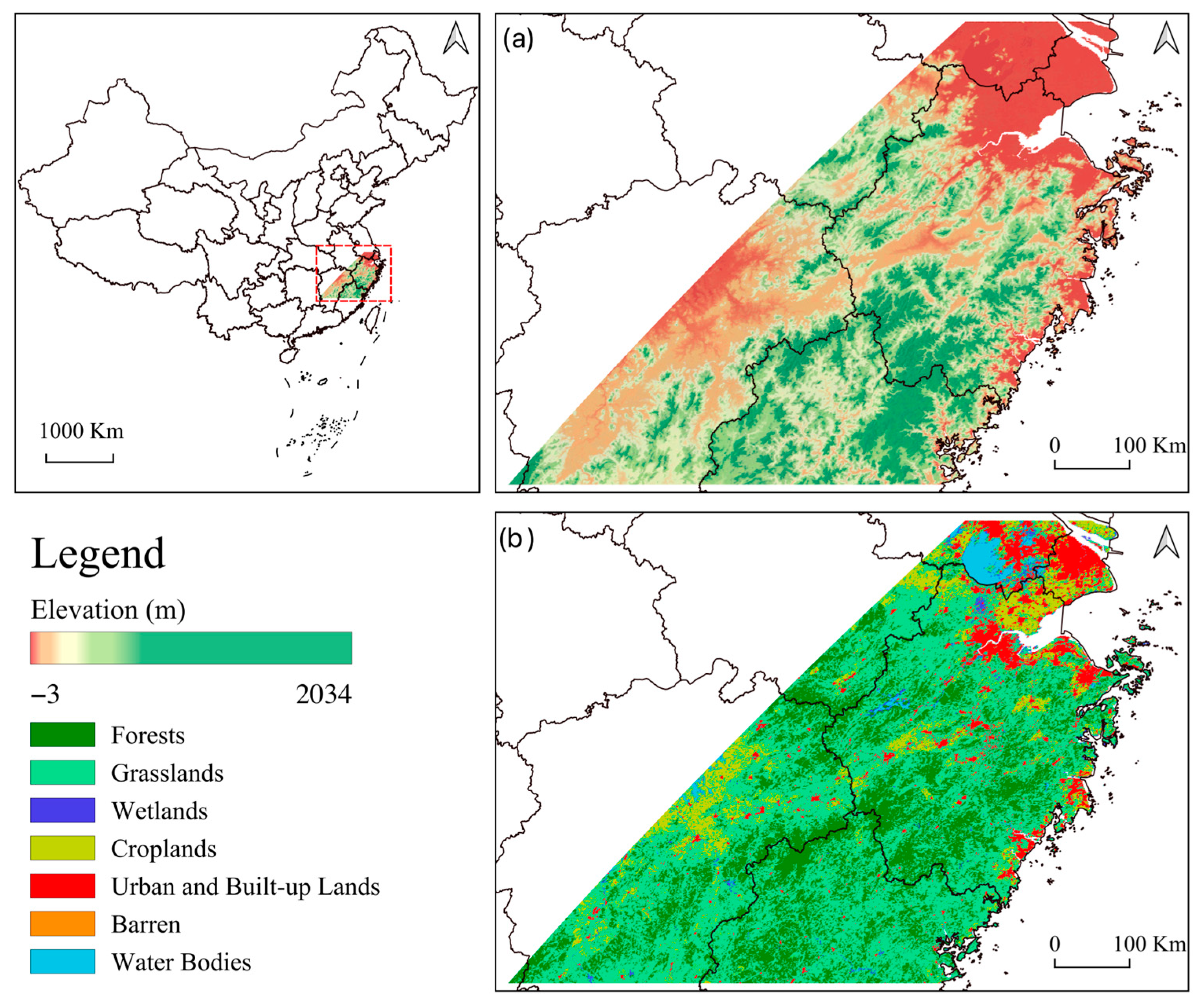
Figure 1 shows the study area (26.25°N–31.66°N, 113.83°E–122.82°E), which is located in southeastern China, including the entire range of Zhejiang province and its surrounding areas, with an area of approximately 261,200 km2. The landcover types in the study area are complex, including mountains, urban buildings, forests, orchards, farmland, lakes and rivers, with a large undulating terrain ranging from an altitude of −3 m to 2034 m. The climate type is subtropical monsoon, and it is located in a humid area, with an average annual temperature ranging from 15 °C to 18 °C and an average annual precipitation of 1000–2000 mm. The four seasons are distinct, with an average temperature of about 15–20 °C in spring and autumn and a maximum temperature above 35 °C in summer, while the lowest temperature drops to 0 °C in winter [31]. In mid-April, there may be a cold wave with sudden temperature drops accompanied by precipitation. If the rainy season lasts from May to July, it may cause more than two consecutive months of satellite image cloud cover, bringing difficulties to the reconstruction of LSTs.
2.2. Satellite Data and Preprocessing
The daily 1 km LST dataset used in this study is the sixth version product released by the Level-1 and Atmosphere Archive & Distribution System Distributed Active Archive Center (LAADS DAAC) and includes MOD11A1 and MYD11A1, which are retrieved from the Moderate Resolution Imaging Spectroradiometer (MODIS) carried on the Terra and Aqua satellites, respectively [32,33]. The Terra satellite was launched in 1999, with observations conducted twice a day at 10:30 a.m. and 10:30 p.m., while the Aqua satellite was launched in 2002, with observations conducted twice a day at 1:30 a.m. and 1:30 p.m. Previous research has demonstrated that the above products are reliable, with errors within 1 K [14]. Two MODIS tiles (h28v05, h28v06) covering the entire study area were obtained from the Earthdata website (https://ladsweb.modaps.eosdis.nasa.gov/search/, accessed on 28 January 2023), with a time range from 25 February 2000 to 15 November 2022 for Terra and from 4 July 2002 to 31 December 2022 for Aqua. The original sinusoidal coordinate system was maintained throughout the data processing, with mosaicking and cropping performed to extract the study area, resulting in 650 rows and 650 columns with approximately 300,000 study area pixels. Then, we converted the units to Celsius. Both MOD11A1 and MYD11A1 products have quality-control (QC) layers that record image quality information. In the preprocessing step, two sets of LST data were generated, named LST images of good-quality pixels (GQ-pixel LST images) and LST images of both good-quality and other-quality pixels (GQ+OQ-pixel LST images). GQ-pixel LST images were obtained by filtering out other-quality pixels, leaving only images containing good-quality pixels. GQ+OQ-pixel LST images were images that include both good-quality pixels and other-quality pixels. The model established using GQ-pixel LST images is called ModelGQ and the model established using GQ+OQ-pixel LST images is called ModelGQ+OQ.
Figure 2 shows the proportions and distribution patterns of the valid data during the study period. The average proportion of valid data for Terra-day, Aqua-day, Terra-night, and Aqua-night in GQ-pixel LST images are 16%, 13%, 17%, and 17%, respectively. The average proportion of valid data for Terra-day, Aqua-day, Terra-night, and Aqua-night in GQ+OQ-pixel LST images are 27%, 26%, 27%, and 28%, respectively. In the picture, the areas with a redder color indicate a lower proportion of valid data, reaching a minimum of 0%, meaning that there is no valid data available throughout the entire study period. On the other hand, the areas with a greener color indicate a higher proportion of valid data, reaching a maximum of 41%. Figure 3 shows the proportion of valid data in LST images across different years. It is evident that the proportion of valid data in GQ+OQ-pixel LST images is significantly higher than that in GQ-pixel LST images. Although there are slight differences across different years, the proportion of valid data in GQ-pixel LST images is generally below 20%, and the proportion of valid data in GQ+OQ-pixel LST images is generally below 40%, indicating that the data has a serious issue with missing values.
The SRTM3 DEM data used in this study were generated from surface elevation data obtained by radar equipment carried on board space shuttles by the National Aeronautics and Space Administration (NASA) and the National Imagery and Mapping Agency (NIMA). These data covered a total area of over 119 million square kilometers between the latitudes of 60 degrees North and 60 degrees South, covering more than 80% of the earth’s land surface with a spatial resolution of 90 m [34]. We downloaded the complete coverage of the study area SRTM3 products from Earthdata (https://lpdaac.usgs.gov/products/srtmimgmv003/, access on 21 July 2022), then carried out mosaicking, resampling, reprojection, clipping, and calculated the slope to obtain the elevation and slope images of the study area with the same resolution as the LST images. Next, we calculated the latitude and longitude coordinates of each pixel using ARCGIS. These data provide important information for LST reconstruction.
2.3. Methods
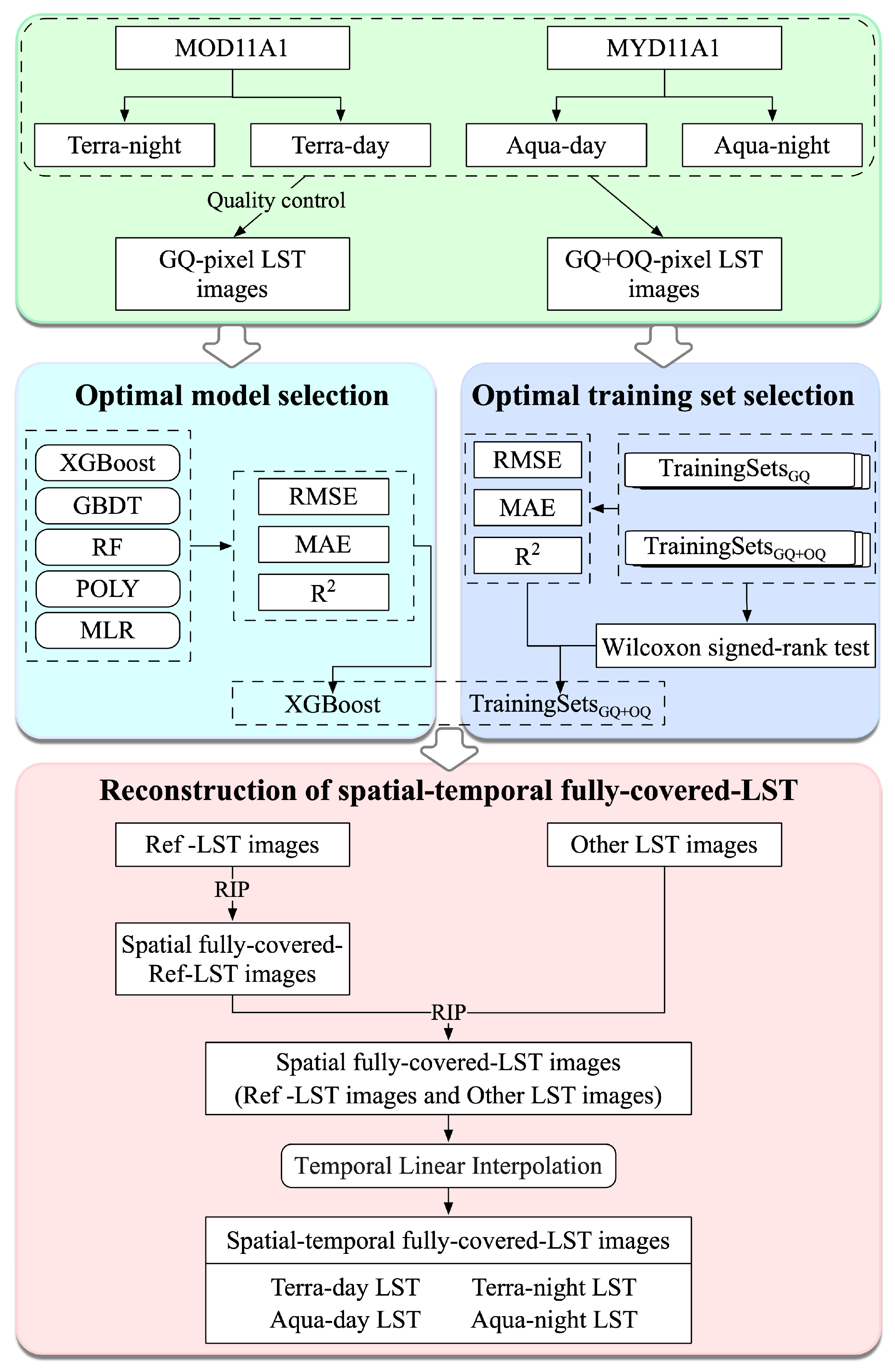
We used five variables for the LST reconstruction, which are the LSTs of the nearest date, longitude, latitude, elevation, and slope. According to the research results of Sun et al., there is a correlation between LSTs with dates that are close to each other [20]. The shorter the time interval between two days, the stronger the correlation between the LST of the two days. Therefore, LSTs from the nearest dates were selected as variables for reconstructing the LST. Longitude and latitude were selected for LST reconstruction because they provide location information. This is based on the Tobler’s First Law of Geography that everything is related to everything else, but neighboring things are more related to each other [35]. Furthermore, elevation and slope are also considered important variables in LST reconstruction due to their strong correlation with LST. Figure 4 shows the flow chart of the LST spatiotemporal reconstruction, which mainly consists of two parts. The first part is the reconstruction of the reference LST image. Firstly, the reference LST images that meet the conditions are selected, and then they are interpolated to achieve full spatial coverage. In this process, the two sets of datasets are modeled on five models respectively. Their performances are compared, and the optimal dataset and model are used to estimate the missing LST values. The second part is the reconstruction of other LST images, which is achieved using the latest dated reference LST image that has already been reconstructed. Finally, the dataset of LSTs that covers both the time and space entirely is obtained using the time interpolation algorithm.
2.3.1. Reference LST Images
The selection of reference LST images has a significant impact on the final reconstruction results because they will be used for the reconstruction of other LST images in later steps. When selecting reference LST images, two factors need to be considered comprehensively: (i) the coverage rates of the reference LST image should be as high as possible; (ii) the date of the reference LST images taken by other images should be as close as possible. If a higher coverage is required for the reference LST images, fewer reference LST images will be selected, resulting in longer date intervals between the reference LST images taken for other LST images. The longer the interval between two days, the lower the correlation of LST between the two days, leading to poor reconstruction accuracy. If the coverage of reference LST images is not required to be higher, it will lead to difficulties in reconstructing the reference LST images and introduce a large amount of error in earlier steps. Therefore, taking into account the above reasons, LST images with a coverage rate no less than 70% were selected as the reference LST imagery, and all other images were considered as other LST images. There were a total of 1841 reference LST images in the GQ-pixel LST images dataset, including 450 LST images in Terra-day, 590 LST images in Terra-night, 339 LST images in Aqua-day, and 462 LST images in Aqua-night. In the GQ+OQ-pixel LST images dataset, there were 4326 reference LST images, including 1125 LST images in Terra-day, 1203 LST images in Terra-night, 899 images in Aqua-day, and 1099 LST images in Aqua-night.
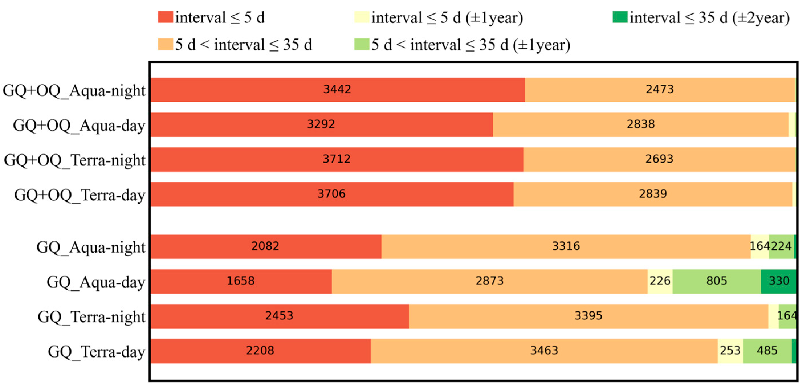
The number of reference LST images in GQ+OQ-pixel LST images is much higher than that in GQ+OQ-pixel LST images. Additionally, the number of GQ-pixel LST reference images at night are 33% more than during the day, and the number of GQ+OQ-pixel LST reference images at night is 14% more than during the day, indicating that there is less cloud cover at night and that the LST retrieved at night is more stable. A 70% coverage threshold not only ensures high coverage of the reference LST image, but also ensures that the date distance between other LST images and their corresponding reference LST images is close enough. Figure 5 shows the date interval between the other LST images and their nearest reference LST images. For the 24,320 other LST images in the GQ-pixel LST images dataset, approximately one-third of them selected reference LST images with an interval of no more than 5 days, and over two-thirds of them selected reference LST images with an interval of no more than 35 days. For the 25,172 other LST images in the GQ+OQ-pixel LST images dataset, approximately one-third of them selected reference LST images with an interval of no more than 5 days, and over 95% of them selected reference LST images with an interval of no more than 35 days. It is not difficult to see that in the GQ+OQ-pixel images, the date interval between other LST images and their corresponding reference LST images is shorter, which may be more favorable for the reconstruction of the LST dataset.
2.3.2. Training Sets and Testing Sets
We split all valid pixels in each image (including reference LST images and other LST images) into training and testing sets with an 8:2 ratio to ensure accurate testing accuracy. Specifically, for each daily LST image, 80% of the GQ pixels are randomly selected as the training sets (TrainingSetsGQ) for ModelGQ, and the remaining 20% are used as the testing set (TestingSetsGQ). 80% of the OQ pixels are randomly selected and combined with the TrainingSetsGQ to form training sets (TrainingSetsGQ+OQ) for ModelGQ+OQ, and the remaining 20% of the OQ pixels are used as the test sets (TestingSetsOQ). TestingSetsGQ+OQ is obtained by merging TestingSetsOQ with TestingSetsGQ. In the end, two training sets were obtained, namely TrainingSetsGQ and TrainingSetsGQ+OQ, along with three testing sets, namely TestingSetsGQ, TestingSetsOQ, and TestingSetsGQ+OQ.
2.3.3. Reconstruction Models and Hyperparameter Optimization
In addition to the impact brought by different training sets, the choice of different interpolation models can also lead to different results. Many studies have employed machine-learning models to accomplish LST reconstruction tasks, which have had high performance, gradually replacing traditional linear models [22,23,24]. In this study, the performance and results of the XGBoost, GBDT, RF, POLY, and MLR models were compared with regard to their reconstruction of LSTs.
Multiple linear regression (MLR) is a common statistical method used to establish a linear relationship model between a dependent variable and multiple independent variables in order to estimate the target. Specifically, the dependent variable can be represented as a linear combination of independent variables, where each independent variable has a corresponding coefficient. These coefficients represent the degree of influence of each independent variable on the dependent variable, also known as regression coefficients. By performing regression analysis on known data, we can obtain the degree of influence of each feature on the LST and use this information to estimate the missing LST values.
Polynomial regression (POLY) is a common regression analysis method that elevates the dimensionality by performing polynomial transformations on the independent variables, enabling linear models to fit non-linear data. By transforming the independent variables into polynomial terms, we can convert the data from its original low-dimensional space to a higher dimensional space. This dimensionality elevation allows the linear model to better fit non-linear data. An important issue in polynomial regression is how to select the degree of the polynomial. If the degree is too low, the model will be too simple to fit the data well. If the degree is too high, the model may overfit the data, leading to poor generalization performance.
As a powerful machine-learning technique, ensemble learning has been increasingly proven to have stronger learning ability and better performance. Its main branches include the Bagging algorithm and the Boosting algorithm. Random forest (RF), as the representative of the bagging algorithm, has been widely used in various fields including remote sensing. RF is designed and proposed based on the decision-tree algorithm, which improves the problem of model overfitting by simultaneously constructing multiple decision trees and introducing randomness [36]. The randomness of random forests is reflected in two aspects: one is to randomly sample with replacement, and the other is to randomly sample without replacement features. This makes random forests highly robust and able to effectively mitigate overfitting problems.
Different from the RF, boosting algorithms construct a series of weak estimators one after another and combine the results of all weak estimators to obtain the final prediction. The basic process is as follows: based on the result of the previous weak estimator f(x)t−1, calculate the loss function L(x, y) and use L(x, y) to adaptively affect the construction of the next weak estimator f(x)t [37]. The integrated model output results are affected by all weak estimators f(x)0~f(x)T. Compared with earlier boosting algorithms (such as Adaboost), the Gradient-boosting decision tree (GBDT) has the following characteristics: no matter whether the GBDT performs classification or regression tasks, the weak estimator must be a regression tree; the loss function can be extended to any differentiable function; and the GBDT affects the structure of subsequent weak estimators by fitting pseudo-residuals (the difference between the current integrated output result and the true label), which can make the loss function reduce the fastest [38].
The Extreme Gradient-Boosting (XGBoost) algorithm has made significant improvements based on the basic modeling process of the Boosting algorithm. These improvements include adding structural risk to the loss function, making them part of the objective function, pursuing the minimum value of the objective function instead of the minimum value of the loss function in the process of building evaluators, achieving a balance between empirical and structural risks, and using information gain as the splitting indicator [39]. These improvements enable the model to have a strong learning ability and overfitting resistance, ensuring accuracy while controlling model complexity and improving computational efficiency.
The performance of an algorithm is greatly influenced by hyperparameters, especially for machine-learning algorithms. To achieve optimal model performance and to reconstruct more accurate LSTs, the selection of hyperparameters is necessary. However, as hyperparameters affect each other, selecting hyperparameters one by one often leads to poor results. Therefore, this study uses a method based on Tree-structured Parzen Estimator (TPE) to select the best hyperparameters. TPE is a probabilistic model-based optimization method that optimizes hyperparameters by constructing a tree-structured probabilistic model [40]. In each iteration, the TPE calculates new hyperparameter values based on the evaluated model performance and the distribution of hyperparameter values and uses them to train new models. Through repeated iterations, the TPE can find the best combination of hyperparameters to improve model performance. The entire process of modeling and hyperparameter optimization is implemented using the Python language’s “scikit-learn” library, “xgboost” library, and “hyperopt” library. Note that since the MLR algorithm has no hyperparameters, it has not been optimized with hyperparameters. Table 2 shows the hyperparameter combinations of each model selected by the TPE algorithm.
2.3.4. Spatial Reconstruction of LSTs
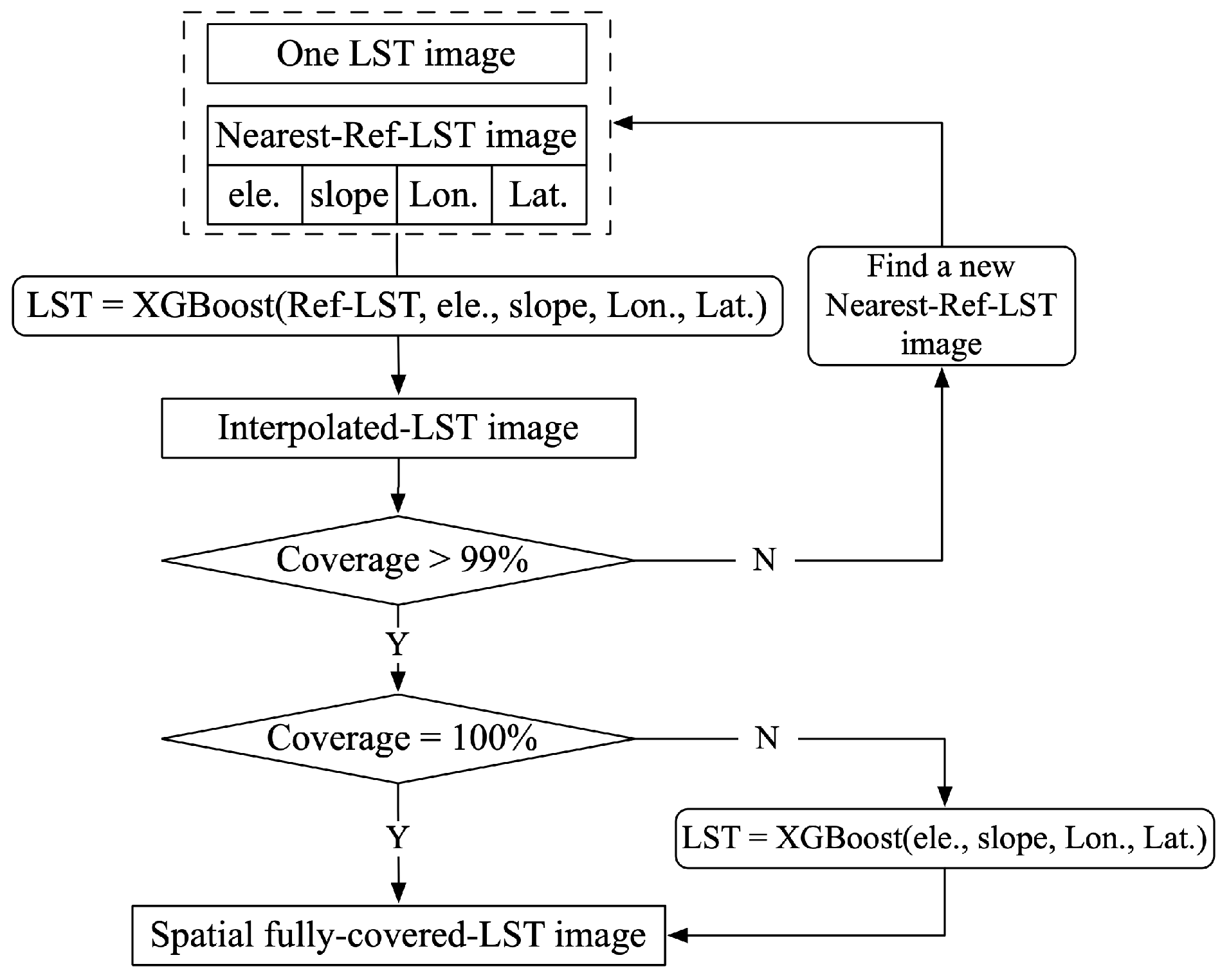
It is insufficient for a single interpolation step to complete the reconstruction of LST. As shown in Figure 6, a Recurrent Interpolate (RIP) method is proposed to achieve full spatial coverage of the LST images. After dividing the reference LST image and other LST images, RIP is used to interpolate the reference LST image and other LST images to achieve the full spatial coverage of both. As shown in Figure 4, the steps of RIP are as follows: for any LST image to be interpolated, select the nearest reference LST image as one of the features, combine this with altitude, slope, longitude, and latitude to establish a model and perform the interpolation once. The result obtained is called the interpolated-LST image. If the coverage of the interpolated LST image is still below 99%, then another Ref-LST image is selected, and a model is established again to carry out another interpolation based on the interpolated-LST image. This process is repeated until the coverage of the obtained interpolated-LST image reaches 99%. Then, only the four features of altitude, slope, longitude, and latitude are used to establish the model to ensure full spatial coverage of this image. Note that if the coverage reaches 100% during any interpolation process, the results are output directly.
In the interpolation process of reference LST images, due to the presence of gaps in the selected reference LST image, after one interpolation, it is impossible to raise the coverage of the interpolated-LST image to 100%. Therefore, multiple interpolations are needed to increase the coverage. In addition, a very small portion of pixels (<1%) cannot be reconstructed during the interpolation process. Consequently, after the coverage is raised to 99%, only seamless terrain and position features are used for interpolation to achieve complete spatial coverage. For other LST images, however, since the full spatial coverage of all reference LST images has been completed, the coverage of the selected reference LST image must be 100%. By combining the five features of reference LST, altitude, slope, longitude, and latitude, only one interpolation is needed to achieve complete spatial coverage.
2.3.5. Accuracy Evaluation
In this study, the clear-sky LSTs in cloudy areas were obtained through an interpolation model, ignoring the influence of clouds on the LST. Therefore, it is inappropriate to compare the reconstructed LSTs with ground observation data, which is affected by clouds. It is more appropriate to select a portion of true values from the image as the test set before training the model. These pixels are not involved in model construction, and the estimated values of the model are compared with the true values to evaluate the performance of the model. TestingSetsGQ, TestingSetsOQ, and TestingSetsGQ+OQ mentioned in Section 2.3.2 will be used to evaluate the accuracy of each LST image. The Root Mean Square Error (RMSE), Mean Absolute Error (MAE), and R2 indicators were calculated, and their calculation formulas are shown below:
where is the number of reconstructed pixels of the current LST image, represents the true LST of pixel i, and represents the LST estimated by the model for pixel i. The lower RMSE and MAE values of the test set indicate higher model accuracy, while a higher R2 represents a stronger model-fitting ability. RMSE, MAE, and R2 were calculated using the metrics “module” of the “sklearn” library.
The Wilcoxon signed-rank test was used to evaluate the difference between reconstructed LSTs and true LSTs on the TestingSetsGQ, TestingSetsOQ, and TestingSetsGQ+OQ datasets. This is a non-parametric test method for comparing two paired samples to determine whether two populations have the same median. Its greatest advantage is that it does not require data to follow normal distribution or homogeneity of variance, which may occur in LST data, in which case the t-test is not suitable. The Wilcoxon signed-rank test helps to select better training sets for LST reconstruction, and this test is implemented through “scipy” library.
3. Results
3.1. Optimal Model for LST Reconstruction
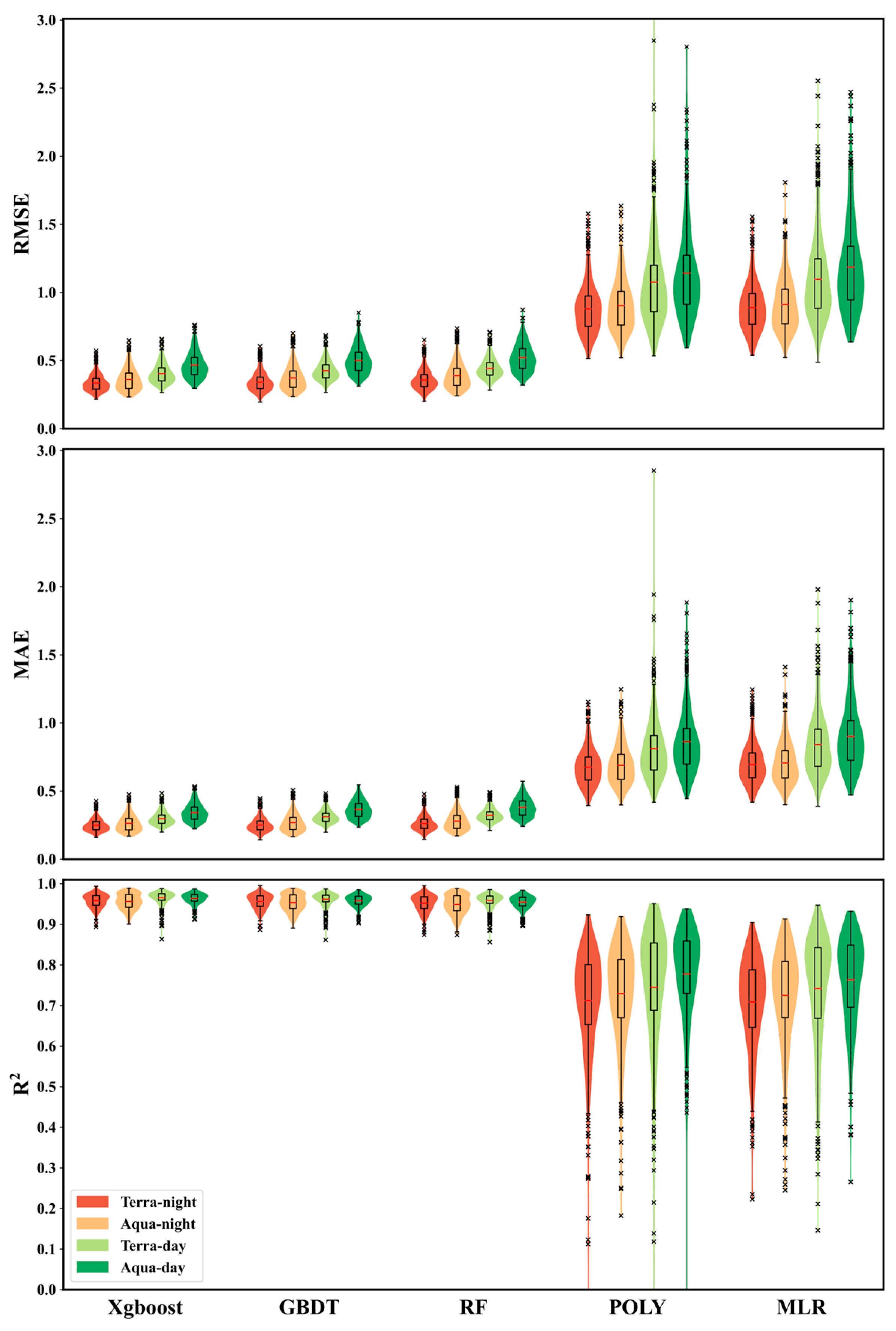
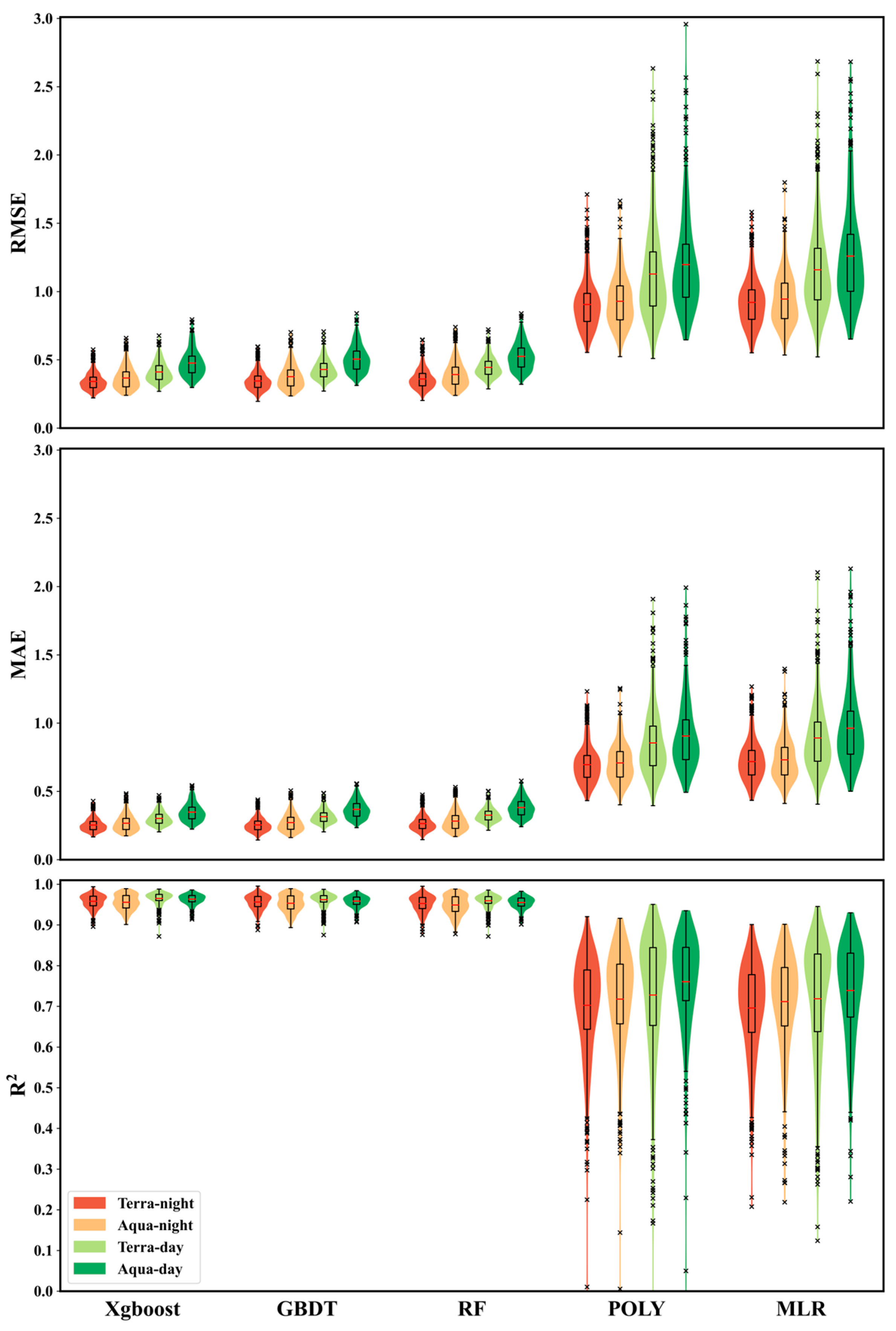
We built the XGBoost, GBDT, RF, POLY, and MLR models using TrainingSetsGQ and TrainingSetsGQ+OQ, respectively, and compared their performance. Figure 7 and Figure 8 show that machine-learning models have better performance compared with traditional regression models. In ModelGQ, the average RMSE of the reconstructed LST obtained by traditional linear regression model is 1.02 °C, the average MAE is 0.78 °C, and the average R2 is 0.73. In contrast, the RMSE of machine-learning models decreased by 60%, the MAE decreased by 62%, and the R2 increased by 32%. Among the three machine learning models, XGBoost performs the best. The model established using the TrainingSetsGQ has an average RMSE of 0.39 °C, an average MAE of 0.29 °C, and an average R2 of 0.96. The model established using the TrainingSetsGQ+OQ has an average RMSE of 0.40 °C, an average MAE of 0.29 °C, and an average R2 of 0.96. Based on these three indicators, there was no significant difference between the models established using TrainingSetsGQ and TrainingSetsGQ+OQ. To sum up, the XGBoost model will be used for subsequent reconstruction processes.
During the reconstruction process of the reference LST image, due to gaps in the reference LST image, which is one of the modeling variables, it is impossible to use reference LST as a feature to achieve full spatial coverage. Therefore, for the small percentage of pixels that have never been interpolated (less than 1%), only four variables, including altitude, slope, longitude, and latitude, are used to build the model, in order to achieve full spatial coverage of the reference LST images. Figure 9 shows that when the coverage is high enough (greater than 70%), whether using TrainingSetsGQ or TrainingSetsGQ+OQ to build the models, removing the reference LST variable results in a slight decrease in model performance, but it is still acceptable.
3.2. Optimal Datasets for LST Reconstruction
As shown in Figure 6 and Figure 7, there is almost no difference in the RMSE, MAE, and R2 between ModelGQ and ModelGQ+OQ. Therefore, it is difficult to decide which dataset performs better. We conducted a Wilcoxon signed-rank test by comparing the number of days with significant differences between the true LST values and the predicted LST values by ModelGQ and ModelGQ+OQ to determine which dataset performs better. Table 3 shows that on whichever test set, ModelGQ+OQ has fewer dates with significant differences between the reconstructed LSTs and true LSTs compared with ModelGQ. This is especially the case for TestingSetsGQ and TestingSetsGQ+OQ, which means that the LST reconstructed by ModelGQ+OQ is closer to the true LST. In subsequent reconstruction steps, TrainingSetsGQ+OQ was chosen as the training sets for LST reconstruction.
3.3. Reconstruction of LST Images
The above results indicated that using TrainingSetsGQ+OQ as the training dataset to establish the XGBoost model can achieve better reconstruction results. Therefore, 4326 reference LST images were reconstructed using TrainingSetsGQ+OQ as the training dataset on the XGBoost model, and the accuracy was evaluated on TestingSetsGQ. Table 4 shows the reconstruction performance at Terra-day, Aqua-day, Terra-night, Aqua-night. The model that used reference LSTs as a feature demonstrated better accuracy compared to the model that did not include reference LST as a feature, as evidenced by a lower RMSE and MAE and a higher R2. The model without reference LST as a feature has slightly lower accuracy, but due to only a small number of missing pixels (less than 1%) being reconstructed by this model, the overall RMSE, MAE, and R2 values are almost identical to those of the model using reference LST as a feature. The reconstruction accuracy at night was better than during the day, and the accuracy of the Terra satellite was superior to that of Aqua. In addition, the study found that the Terra-night LST has the highest accuracy with an RMSE of 0.36 °C, an MAE of 0.26 °C, and an R2 of 0.95, while the Aqua-day LST has the lowest accuracy with an RMSE of 0.61 °C, an MAE of 0.43 °C, and an R2 of 0.95.
After completing the spatial coverage of reference LST images, the RIP was used to reconstruct 22,033 other LST images, including 5743 Terra-day, 5613 Terra-night, 5371 Aqua-day, and 5306 Aqua-night. Table 5 shows the reconstruction accuracy on the other LST images. Consistent with the reconstruction results of the reference LST image, the interpolation accuracy is higher at night than during the day, and Terra satellite has higher interpolation accuracy than Aqua satellite. The accuracy of Terra-night LST has the highest accuracy with an RMSE of 0.49 °C, MAE of 0.32 °C, and R2 of 0.95, while the accuracy of the Aqua-day LST is the lowest, with an RMSE of 0.83 °C, MAE of 0.57 °C, and R2 of 0.92.
After completing the steps mentioned above, the proportion of valid data had increased to approximately 80% (Figure 10), but some of the LST images were still incomplete, including 1260 LST images in Terra-day, 1096 LST images in Aqua-day, 1306 LST images in Terra-night, and 957 LST images in Aqua-night. This is because (i) the LST products of some dates were not produced for various reasons, making it impossible to obtain them from the official website. (ii) Although some dates have LST products available from the official website, the number of good-quality and other-quality pixels in the image is 0, which makes it impossible to build an XGBoost model to reconstruct LSTs; iii) in the images of other dates, the number of good-quality and other-quality pixels is too low (less than 0.25% [41]) to build a model, and the LST data for these dates have therefore not been reconstructed. Therefore, a weighted averaging algorithm based on the distance between dates is used to reconstruct the LST missing over time, with the specific formula as follows:
where represents the reconstructed LST of pixel i on the current date. is the LST of pixel i on the latest date before the current date. is the LST of pixel i on the latest date after the current date. is the number of days between and , and is the number of days between and .
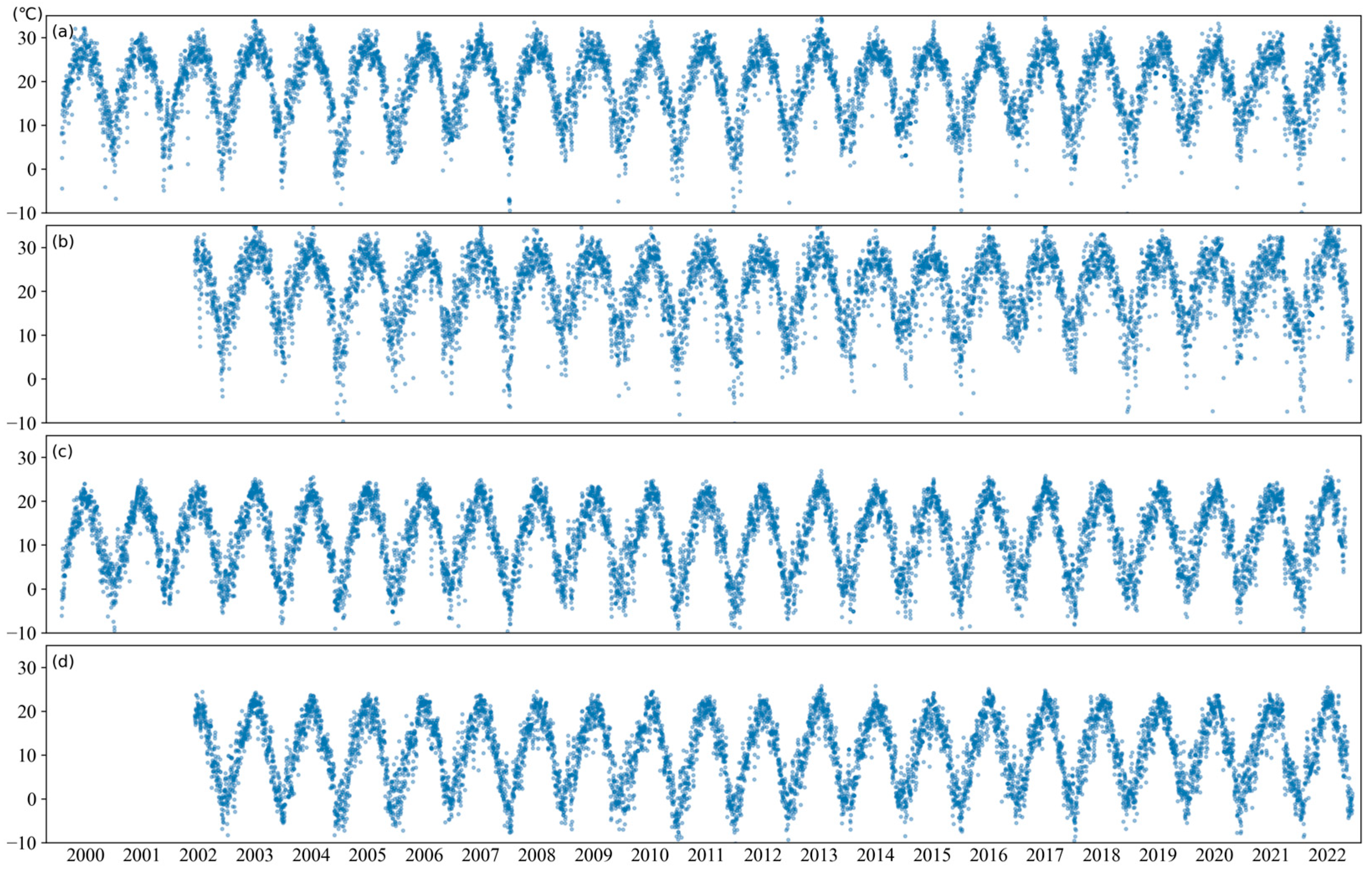
After completing all the reconstruction steps, a seamless 1 km LST dataset in Zhejiang and its surrounding area from 2000 to 2022 was obtained, which included 8300 LST images in Terra-day, 7485 LST images in Aqua-day, 8300 LST images in Terra-night, and 7485 LST images in Aqua-night. Then, we calculated the average LST within the study area for each image and observed the variations in LSTs at daily, monthly, and yearly scales. The fluctuations observed were consistent with expectations and aligned with common patterns (Figure 11, Figure 12 and Figure 13).
4. Discussion
4.1. Machine Learning in LST Reconstruction
The development of machine learning is now evident and is increasingly being applied in remote-sensing research, such as in the reconstruction of LST. Traditional linear regression models, such as multiple linear regression models, are simple and time saving but lack the ability to learn from data and to capture complex deep relationships between the LST and related variables, which may be nonlinear. With the development of tree models, ensemble models such as RF, GBDT, XGBoost and others have outperformed traditional models with their strong learning ability, high resistance to overfitting, and other advantages. Fan et al. reconstructed LSTs using a linear regression model with an RMSE of 1.85 K; they also reconstructed LSTs using a regression decision-tree model with an RMSE of 1.32 K, and they utilized an artificial neural network to reconstruct LST with an RMSE of 1.66 K [21]. Xiao et al. used an RF-based method to reconstruct LST with an RMSE of 2.63 K [22]. Cho et al. employed a LightGBM-based method, achieving an RMSE of 0.6 °C at nighttime and 1.1–1.4 °C at daytime for the LST reconstruction [24]. In this study, the LST was reconstructed using the XGBoost model, resulting in an RMSE of 0.36–0.83 °C. This performance was found to be superior to that of other studies. In addition to the modeling performance brought by machine-learning models themselves, selecting appropriate features is also an indispensable part of LST reconstruction work. Tan et al. selected CLDAS data and other surface attribute factors to reconstruct LST through XGBoost with an RMSE of 4 K [23]. In this study, a reference LST was added as one of features for reconstructing LSTs, resulting in an average RMSE reduction of less than 1 K after reconstruction. Furthermore, unlike traditional regression models, the selection of hyperparameters is crucial when using XGBoost to reconstruct the LST, and optimizing hyperparameters can significantly improve the model’s performance. Compared with the XGBoost default parameters, the average RMSE decreased by about 50% after hyperparameter optimization. In summary, selecting suitable models for LST reconstruction, stronger features related to LST, and appropriate hyperparameters can greatly improve the accuracy of LST reconstruction and enhance the robustness of reconstruction work.
4.2. Dataset for Model Training
Many studies in LST reconstruction have only used good-quality pixels, resulting in a reconstructed LST dataset with an RMSE greater than 1 K [17,18,20,28,30]. In contrast, our reconstructed LST dataset has an RMSE controlled within 1 K. Therefore, solely excluding the so-called “low-quality pixels” through QC layers is not conducive to LST reconstruction. This may be attributed to the following reasons. On the one hand, some cities such as Shanghai have no good-quality pixels from 2000–2022, and the pixel values in those locations are classified as “other-quality”, with an average emissivity error ≤ 0.02 in quality-control layers. This means that the reconstructed LST in these areas comes from models that remove reference LSTs using four terrain and location features, resulting in lower accuracy and potentially less reliability compared with LST images with other-quality pixels. On the other hand, using only GQ pixels results in more dates with completely missing LST images, which rely on time-weighted averages. The accuracy of these results is uncertain and difficult to validate. In contrast, using both good-quality and other-quality pixels increases the daily coverage, reduces the number of completely missing pixels, and provides more reference LST images. It also decreases the time interval between other LST images and the reference LST, improving model performance. Furthermore, using all the valid pixels increases the sample size during model building, which can enhance the robustness of the model.
4.3. Spatial–Temporal Pattern of LST
Figure 14 displays the spatial patterns of the average values of LST for different pixels during the study period. Due to solar radiation and the complexity of the underlying surface, the LST in built-up areas is higher and spatially heterogeneous during the daytime. In contrast, the LST in water bodies, such as Tai Lake, is lower and spatially homogeneous. In mountainous areas, LST is primarily influenced by elevation, with higher altitudes corresponding to lower LST values. Among the four observation times, Aqua-day has the highest LST, with an average LST of 21.2 °C in the study area and average LSTs of different pixels ranging from 15 °C to 26 °C. Terra-day comes next, with an average LST of 19.7 °C in the study area and average LSTs of different pixels ranging from 15 °C to 23 °C. Terra-night ranks third, with an average LST of 11.6 °C in the study area and average LSTs of different pixels ranging from 8 °C to 14 °C. Aqua-night has the lowest LST, with an average LST of 11.0 °C in the study area and average LSTs of different pixels ranging from 7 °C to 13 °C, which is consistent with the temperature diurnal cycle.
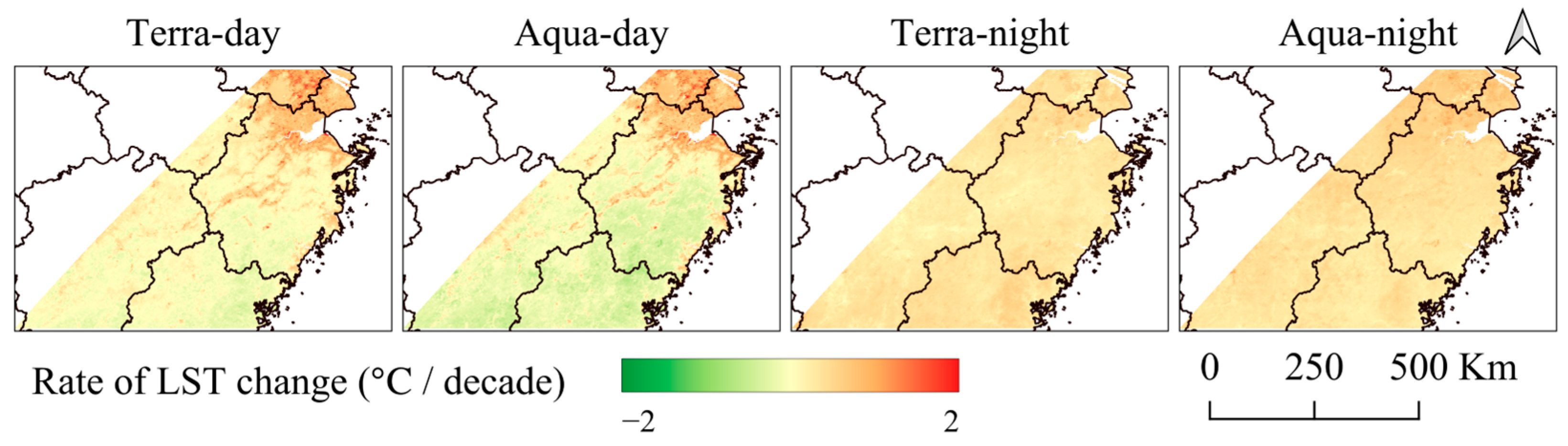
Calculating the slopes of different pixels during the study period, we obtained the temporal trends of LST. As shown in Figure 15, LST shows a gradual upward trend from 2000 to 2022, especially in urban and built-up areas during the daytime, which is attributed to recent urban expansion. An increase in LST leads to changes in precipitation patterns, resulting in a noticeable increase in the frequency and intensity of extreme weather and climate events such as heatwaves, extreme droughts, and flooding [42]. This could have a potential impact on the entire ecosystem.
4.4. Application of Reconstructed LSTs in High-Temperature Monitoring
The Aqua satellite observes during the daytime at 1:30 pm, which can be considered the approximate time when the highest temperature of the day occurs. Therefore, it is often used for high-temperature monitoring. We used the reconstructed Aqua-day LST data to calculate the number of days during each summer (June to September) of every year with the highest LST exceeding 35 °C. Figure 16 displays the results for the years 2013, 2020, 2021, and 2022. From the figure, we can see that the summer temperatures in 2020 and 2021 were lower compared with other years due to fewer hot regions and shorter high-temperature periods. In contrast, the summers of 2013 and 2022 were significantly hotter, with some areas experiencing more than 70 days with LSTs exceeding 35 °C. These findings are consistent with news reports and the results of other researchers. A study shows that 2022 was the hottest summer on record in China, which was due to the extremely strong and westwardly-expanded Western Pacific subtropical high [43]. In conclusion, LST datasets like this are highly suitable for high-temperature monitoring, enabling timely detection of areas most severely affected by heat, and providing guidance for government decision-making.
5. Conclusions
Thermal infrared remote sensing enables the creation of high-precision, high-spatiotemporal-resolution, and large-coverage LST dataset products. However, the gaps caused by cloud contamination in the images limit the application of such products. In this study, we found that modeling using both good-quality and other-quality pixels in MODIS LST data exhibits better reconstruction performance than using only good-quality pixels. This is because there is still a significant amount of useful information in these pixels, and it is inappropriate to discard them. Additionally, the XGBoost model demonstrated stronger learning capabilities and was adept at fitting more complex relationships compared with the other four models. Therefore, the TrainingSetsGQ+OQ and XGBoost models were chosen to reconstruct daily 1 km LSTs for Zhejiang Province and its surrounding areas from 2000 to 2022, which provided four daily observations at 10:30 a.m., 1:30 p.m., 10:30 p.m., and 1:30 a.m. with an average RMSE < 1 °C, MAE < 1 °C, and R2 > 0.9.
This study provides an effective method for solving the problem of missing LST data, which is helpful for the reconstruction of LSTs in larger areas and has positive significance for crop monitoring and climate change research.
Author Contributions
Conceptualization, Y.X. and R.H.; methodology, Y.X., S.L., J.H. and R.H.; software, S.L.; validation, Y.X. and S.L.; formal analysis, R.H.; investigation, Y.X.; resources, Y.X. and S.L.; data curation, S.L. and C.Z.; writing—original draft preparation, Y.X. and S.L.; writing—review and editing, Y.X., R.H. and J.H.; visualization, Y.X. and C.Z.; supervision, J.H.; funding acquisition, R.H. and J.H. All authors have read and agreed to the published version of the manuscript.
Funding
This research was funded by the National Natural Science Foundation of China (Grant No. 42101364), the Zhejiang Provincial Natural Science Foundation (Grant No. LQ21D010006), and the Project Supported by the Key R&D Program of Zhejiang Province (Grant No. 2021C02036).
Data Availability Statement
Data are available from the corresponding authors upon request.
Conflicts of Interest
The authors declare that they have no known competing financial interest or personal relationships that could have appeared to influence the work reported in this paper.
References
- Friedl, M.A. Forward and Inverse Modeling of Land Surface Energy Balance Using Surface Temperature Measurements. Remote Sens. Environ. 2002, 79, 344–354. [Google Scholar] [CrossRef]
- Pede, T.; Mountrakis, G.; Shaw, S.B. Improving Corn Yield Prediction across the US Corn Belt by Replacing Air Temperature with Daily MODIS Land Surface Temperature. Agric. For. Meteorol. 2019, 276, 107615. [Google Scholar] [CrossRef]
- Zhou, D.; Xiao, J.; Bonafoni, S.; Berger, C.; Deilami, K.; Zhou, Y.; Frolking, S.; Yao, R.; Qiao, Z.; Sobrino, J.A. Satellite Remote Sensing of Surface Urban Heat Islands: Progress, Challenges, and Perspectives. Remote Sens. 2019, 11, 48. [Google Scholar] [CrossRef]
- Islam, S.; Ma, M. Geospatial Monitoring of Land Surface Temperature Effects on Vegetation Dynamics in the Southeastern Region of Bangladesh from 2001 to 2016. ISPRS Int. J. Geo-Inf. 2018, 7, 486. [Google Scholar] [CrossRef]
- Hijmans, R.J.; Cameron, S.E.; Parra, J.L.; Jones, P.G.; Jarvis, A. Very High Resolution Interpolated Climate Surfaces for Global Land Areas. Int. J. Climatol. 2005, 25, 1965–1978. [Google Scholar] [CrossRef]
- Li, Z.-L.; Tang, B.-H.; Wu, H.; Ren, H.; Yan, G.; Wan, Z.; Trigo, I.F.; Sobrino, J.A. Satellite-Derived Land Surface Temperature: Current Status and Perspectives. Remote Sens. Environ. 2013, 131, 14–37. [Google Scholar] [CrossRef]
- Gao, H.; Fu, R.; Dickinson, R.E.; Juarez, R.I.N. A Practical Method for Retrieving Land Surface Temperature from AMSR-E over the Amazon Forest. IEEE Trans. Geosci. Remote Sens. 2008, 46, 193–199. [Google Scholar] [CrossRef]
- Yang, H.; Weng, F. Error Sources in Remote Sensing of Microwave Land Surface Emissivity. IEEE Trans. Geosci. Remote Sens. 2011, 49, 3437–3442. [Google Scholar] [CrossRef]
- Lian, Y.; Duan, S.-B.; Huang, C.; Han, W.; Liu, M. Generation of Spatial-Seamless AMSR2 Land Surface Temperature in China During 2012–2020 Using a Deep Neural Network. IEEE Trans. Geosci. Remote Sens. 2023, 61, 5300618. [Google Scholar] [CrossRef]
- Qin, Z.; Karnieli, A.; Berliner, P. A Mono-Window Algorithm for Retrieving Land Surface Temperature from Landsat TM Data and Its Application to the Israel-Egypt Border Region. Int. J. Remote Sens. 2001, 22, 3719–3746. [Google Scholar] [CrossRef]
- Jimenez-Munoz, J.C.; Sobrino, J.A. A Generalized Single-Channel Method for Retrieving Land Surface Temperature from Remote Sensing Data. J. Geophys. Res.-Atmos. 2003, 108, 4688. [Google Scholar] [CrossRef]
- Wan, Z.M.; Dozier, J. A Generalized Split-Window Algorithm for Retrieving Land-Surface Temperature from Space. IEEE Trans. Geosci. Remote Sens. 1996, 34, 892–905. [Google Scholar] [CrossRef]
- Sobrino, J.A.; Li, Z.L.; Stoll, M.P.; Becker, F. Multi-Channel and Multi-Angle Algorithms for Estimating Sea and Land Surface Temperature with ATSR Data. Int. J. Remote Sens. 1996, 17, 2089–2114. [Google Scholar] [CrossRef]
- Wan, Z. New Refinements and Validation of the Collection-6 MODIS Land-Surface Temperature/Emissivity Product. Remote Sens. Environ. 2014, 140, 36–45. [Google Scholar] [CrossRef]
- Pede, T.; Mountrakis, G. An Empirical Comparison of Interpolation Methods for MODIS 8-Day Land Surface Temperature Composites across the Conterminous Unites States. Isprs J. Photogramm. Remote Sens. 2018, 142, 137–150. [Google Scholar] [CrossRef]
- NourEldeen, N.; Mao, K.; Yuan, Z.; Shen, X.; Xu, T.; Qin, Z. Analysis of the Spatiotemporal Change in Land Surface Temperature for a Long-Term Sequence in Africa (2003–2017). Remote Sens. 2020, 12, 488. [Google Scholar] [CrossRef]
- Fu, P.; Xie, Y.; Weng, Q.; Myint, S.; Meacham-Hensold, K.; Bernacchi, C. A Physical Model-Based Method for Retrieving Urban Land Surface Temperatures under Cloudy Conditions. Remote Sens. Environ. 2019, 230, 111191. [Google Scholar] [CrossRef]
- Zhang, X.; Zhou, J.; Liang, S.; Wang, D. A Practical Reanalysis Data and Thermal Infrared Remote Sensing Data Merging (RTM) Method for Reconstruction of a 1-Km All-Weather Land Surface Temperature. Remote Sens. Environ. 2021, 260, 112437. [Google Scholar] [CrossRef]
- Yao, R.; Wang, L.; Huang, X.; Cao, Q.; Wei, J.; He, P.; Wang, S.; Wang, L. Global Seamless and High-Resolution Temperature Dataset (GSHTD), 2001–2020. Remote Sens. Environ. 2023, 286, 113422. [Google Scholar] [CrossRef]
- Sun, L.; Chen, Z.; Gao, F.; Anderson, M.; Song, L.; Wang, L.; Hu, B.; Yang, Y. Reconstructing Daily Clear-Sky Land Surface Temperature for Cloudy Regions from MODIS Data. Comput. Geosci. 2017, 105, 10–20. [Google Scholar] [CrossRef]
- Fan, X.-M.; Liu, H.-G.; Liu, G.-H.; Li, S.-B. Reconstruction of MODIS Land-Surface Temperature in a Flat Terrain and Fragmented Landscape. Int. J. Remote Sens. 2014, 35, 7857–7877. [Google Scholar] [CrossRef]
- Xiao, Y.; Zhao, W.; Ma, M.; He, K. Gap-Free LST Generation for MODIS/Terra LST Product Using a Random Forest-Based Reconstruction Method. Remote Sens. 2021, 13, 2828. [Google Scholar] [CrossRef]
- Tan, W.; Wei, C.; Lu, Y.; Xue, D. Reconstruction of All-Weather Daytime and Nighttime MODIS Aqua-Terra Land Surface Temperature Products Using an XGBoost Approach. Remote Sens. 2021, 13, 4723. [Google Scholar] [CrossRef]
- Cho, D.; Bae, D.; Yoo, C.; Im, J.; Lee, Y.; Lee, S. All-Sky 1 Km MODIS Land Surface Temperature Reconstruction Considering Cloud Effects Based on Machine Learning. Remote Sens. 2022, 14, 1815. [Google Scholar] [CrossRef]
- Yu, W.; Tan, J.; Ma, M.; Li, X.; She, X.; Song, Z. An Effective Similar-Pixel Reconstruction of the High-Frequency Cloud-Covered Areas of Southwest China. Remote Sens. 2019, 11, 336. [Google Scholar] [CrossRef]
- Metz, M.; Andreo, V.; Neteler, M. A New Fully Gap-Free Time Series of Land Surface Temperature from MODIS LST Data. Remote Sens. 2017, 9, 1333. [Google Scholar] [CrossRef]
- Zeng, C.; Long, D.; Shen, H.; Wu, P.; Cui, Y.; Hong, Y. A Two-Step Framework for Reconstructing Remotely Sensed Land Surface Temperatures Contaminated by Cloud. Isprs J. Photogramm. Remote Sens. 2018, 141, 30–45. [Google Scholar] [CrossRef]
- Pham, H.T.; Kim, S.; Marshall, L.; Johnson, F. Using 3D Robust Smoothing to Fill Land Surface Temperature Gaps at the Continental Scale. Int. J. Appl. Earth Obs. Geoinf. 2019, 82, 101879. [Google Scholar] [CrossRef]
- Gong, Y.; Li, H.; Shen, H.; Meng, C.; Wu, P. Cloud-Covered MODIS LST Reconstruction by Combining Assimilation Data and Remote Sensing Data through a Nonlocality-Reinforced Network. Int. J. Appl. Earth Obs. Geoinf. 2023, 117, 103195. [Google Scholar] [CrossRef]
- Zhao, X.; Xia, H.; Pan, L.; Song, H.; Niu, W.; Wang, R.; Li, R.; Bian, X.; Guo, Y.; Qin, Y. Drought Monitoring over Yellow River Basin from 2003–2019 Using Reconstructed MODIS Land Surface Temperature in Google Earth Engine. Remote Sens. 2021, 13, 3748. [Google Scholar] [CrossRef]
- Lou, W.; Wu, L.; Mao, Y.; Sun, K. Precipitation and Temperature Trends and Dryness/Wetness Pattern during 1971–2015 in Zhejiang Province, Southeastern China. Theor. Appl. Climatol. 2018, 133, 47–57. [Google Scholar] [CrossRef]
- Wan, Z.; Hook, S.; Hulley, G. MOD11A1 MODIS/Terra Land Surface Temperature/Emissivity Daily L3 Global 1km SIN Grid V006; NASA EOSDIS LP DAAC: Sioux Falls, SD, USA, 2015.
- Wan, Z.; Hook, S.; Hulley, G. MYD11A1 MODIS/Aqua Land Surface Temperature/Emissivity Daily L3 Global 1km SIN Grid V006; NASA EOSDIS LP DAAC: Sioux Falls, SD, USA, 2015.
- NASA JPL. NASA Shuttle Radar Topography Mission Combined Image Data Set; NASA JPL: Pasadena, CA, USA, 2014.
- Tobler, W.R. A Computer Movie Simulating Urban Growth in the Detroit Region. Econ. Geogr. 1970, 46, 234–240. [Google Scholar] [CrossRef]
- Breiman, L. Random Forests. Mach. Learn. 2001, 45, 5–32. [Google Scholar] [CrossRef]
- Freund, Y.; Schapire, R.E. Experiments with a New Boosting Algorithm. In Proceedings of the Thirteenth International Conference on International Conference on Machine Learning, Bari, Italy, 3–6 July 1996; pp. 148–156. [Google Scholar]
- Friedman, J.H. Stochastic Gradient Boosting. Comput. Stat. Data Anal. 2002, 38, 367–378. [Google Scholar] [CrossRef]
- Chen, T.; Guestrin, C. XGBoost: A Scalable Tree Boosting System. In Proceedings of the KDD’16: 22nd Acm Sigkdd International Conference on Knowledge Discovery and Data Mining, San Francisco, CA, USA, 13–17 August 2016; pp. 785–794. [Google Scholar]
- James, B.; Remi, B.; Yoshua, B.; Balazs, K. Algorithms for Hyper-Parameter Optimization; Neural Information Processing Systems: Granada, Spain, 2011. [Google Scholar]
- Colditz, R. An Evaluation of Different Training Sample Allocation Schemes for Discrete and Continuous Land Cover Classification Using Decision Tree-Based Algorithms. Remote Sens. 2015, 7, 9655–9681. [Google Scholar] [CrossRef]
- Utsumi, N.; Seto, S.; Kanae, S.; Maeda, E.E.; Oki, T. Does Higher Surface Temperature Intensify Extreme Precipitation? Geophys. Res. Lett. 2011, 38, L16708. [Google Scholar] [CrossRef]
- Li, X.; Hu, Z.-Z.; Liu, Y.; Liang, P.; Jha, B. Causes and Predictions of 2022 Extremely Hot Summer in East Asia. J. Geophys. Res.-Atmos. 2023, 128, e2022JD038442. [Google Scholar] [CrossRef]
Figure 1.
Map of the study area. (a) Digital elevation model (DEM) of the study area. (b) Land cover map of the study area.
Figure 1.
Map of the study area. (a) Digital elevation model (DEM) of the study area. (b) Land cover map of the study area.

Figure 2.
Proportion and distribution graph of valid values in different datasets. (a–d) correspond to the Terra-day, Aqua-day, Terra-night, and Aqua-night GQ-pixel LST images, respectively. (e–h) correspond to the Terra-day, Aqua-day, Terra-night, and Aqua-night GQ+OQ-pixel LST images, respectively. GQ+OQ-pixel images coverage is more than 10% higher than GQ-pixel images. Some areas in GQ-pixel images (marked in red in the image) do not have any pixels available from 2000 to 2022. The pixel with the highest coverage in GQ+OQ-pixel images has about 41% coverage.

Figure 3.
Polar bar chart of the proportion of valid data in LST images across different years. (a–d) correspond to the Terra-day, Aqua-day, Terra-night, and Aqua-night GQ-pixel LST images, respectively. (e–h) correspond to the Terra-day, Aqua-day, Terra-night, and Aqua-night GQ+OQ-pixel LST images, respectively.

Figure 4.
Flowchart of the reconstruction of the LST dataset.

Figure 5.
The date interval between the other LST image and the nearest reference LST image under different quality control conditions. In GQ+OQ-pixel images, the time interval between the other LST image and its corresponding reference LST image is closer than in GQ-pixel images. Furthermore, most of the other LST images have a date interval with their corresponding reference LST images that does not exceed 35 days (over half of the other-LST images have a date interval of no more than 5 days with their corresponding reference LST images).

Figure 6.
Framework of the Recurrent Interpolate (RIP) method.

Figure 7.
Comparison of the RMSE, MAE, and R2 of the five models built on TrainingSetsGQ. The symbol “x” represents outlier.
Figure 7.
Comparison of the RMSE, MAE, and R2 of the five models built on TrainingSetsGQ. The symbol “x” represents outlier.

Figure 8.
Comparison of RMSE, MAE, and R2 of the five models built on TrainingSetsGQ+OQ. The symbol “x” represents outlier.
Figure 8.
Comparison of RMSE, MAE, and R2 of the five models built on TrainingSetsGQ+OQ. The symbol “x” represents outlier.

Figure 9.
Comparison of the RMSE, MAE, and R2 between the model LST = XGBoost (Ref-LST, ele., slope, Lon., Lat.) and the model LST = XGBoost (ele., slope, Lon., Lat.). When the coverage is high enough, removing the reference LST and modeling using only the other four features results in both ModelGQ and ModelGQ+OQ showing a slight decrease, but this regression is acceptable. The symbol “x” represents outlier.

Figure 10.
Polar bar chart of the proportion of valid data in reconstructed LST images across different years. (a–d) correspond to the Terra-day, Aqua-day, Terra-night, and Aqua-night reconstructed LST images, respectively.
Figure 10.
Polar bar chart of the proportion of valid data in reconstructed LST images across different years. (a–d) correspond to the Terra-day, Aqua-day, Terra-night, and Aqua-night reconstructed LST images, respectively.

Figure 11.
The temporal variation of the reconstructed average LST within the study area over the research period on a daily scale. (a) Terra-day; (b) Aqua-day; (c) Terra-night; (d) Aqua-night.
Figure 11.
The temporal variation of the reconstructed average LST within the study area over the research period on a daily scale. (a) Terra-day; (b) Aqua-day; (c) Terra-night; (d) Aqua-night.

Figure 12.
The temporal variation of the reconstructed average LST within the study area over the research period on a monthly scale.
Figure 12.
The temporal variation of the reconstructed average LST within the study area over the research period on a monthly scale.

Figure 13.
The temporal variation of the reconstructed average LST within the study area over the research period on a yearly scale.
Figure 13.
The temporal variation of the reconstructed average LST within the study area over the research period on a yearly scale.

Figure 14.
The spatial pattern of LST for four observation times.

Figure 15.
The temporal pattern of LST for four observation times.

Figure 16.
The number of days with Aqua-day LSTs exceeding 35 °C in the years 2013, 2020, 2021, and 2022.
Figure 16.
The number of days with Aqua-day LSTs exceeding 35 °C in the years 2013, 2020, 2021, and 2022.


Table 1.
Some research on LST reconstruction.
| Sensors | Time Period Temporal Resolution | Method | Variables | Quality Control | RMSE | References |
|---|---|---|---|---|---|---|
| Terra | 2011–2016 8-day | six interpolation methods | LST, elevation | good quality | 0.2–1.2 °C | [15] |
| Terra/Aqua | 2003–2017 daily | IDW interpolation | LST, elevation | good quality | 0.84 °C | [16] |
| Terra/Aqua | 28 April 2011–20 May 2011 daily | WRFF | LST | good quality | ~2.0 K | [17] |
| Terra/Aqua | 2003 and 2014 daily | RTM | LST, reanalysis data | good quality | 2–4 K | [18] |
| Terra | 2001–2020 8-day | ETD | LST, reanalysis data | not mentioned | 1 K | [19] |
| Terra | 2000–2002 daily | RSDAST | LST | good quality | 1 K | [20] |
| Terra | May, 2005 daily | MLR, RT, ANN | Landcover, NDVI, MODIS band 7 | not mentioned | 1.85 °C, 1.32 °C, 1.66 °C | [21] |
| Terra | 2018 daily | RF-based method | NDVI, EVI, NDWI, elevation, slope, latitude, solar radiation factor | good quality | 2.6 K | [22] |
| Terra/Aqua | Summer of 2017 and 2018 daily | XGBoost-based method | NDVI, EVI, NDWI, elevation, slope, albedo, reanalysis data | error < 2 K | 3.9–5.5 K | [23] |
| Terra/Aqua | 2013–2020 daily | LightGBM-based method | Reanalysis data, elevation, slope, impervious area ratio, wind speed, day of the year, longitude, latitude | good quality | 0.6–1.4 °C | [24] |
| Terra | 2012 daily | energy balance and similar pixels | NDVI, radiation, elevation, slope, aspect | emissivity < 0.04 error < 2 K | 1.9–3.2 K | [25] |
| Terra/Aqua | 2003–2016 daily | temporal and spatial interpolation | LST, elevation, emissivity | error < 3 K | 0.5 K | [26] |
| Terra | 2010 daily | two-step framework | LST, NDVI, radiation | not mentioned | 3–6 K | [27] |
| Aqua | 2002–2011 daily | 3-D gap-filling method | LST | good quality | 2 K | [28] |
| Terra/Aqua | 2019 daily | Nonlocality-reinforced network | LST, NDVI, elevation, reanalysis data | not mentioned | 0.8 K | [29] |
| Aqua | 2003–2019 daily | ATC model | LST, day of the year | good quality | 3 K | [30] |
Table 2.
The optimal combination of hyperparameters for the five models.
| Models | Optimal Hyperparameters |
|---|---|
| MLR | — |
| POLY | degree = 4 |
| RF | n_estimators = 200 max_features = 4 max_depth = 40 criterion = ‘squared_error’ |
| GBDT | n_estimators = 200 learning_rate = 0.06 loss = ‘squared_error’ max_features = 3 subsample = 0.6 max_depth = 18 |
| XGBoost | num_boost_round = 200 eta = 0.1 colsample_bytree = 5/6 lambda = 0.7 max_depth = 18 subsample = 0.9 |
Table 3.
The Wilcoxon signed-rank test results for the LST estimate values of ModelGQ and ModelGQ+OQ on three test sets (TestingSetsGQ, TestingSetsOQ, TestingSetsGQ+OQ). “SD” refers to the proportion of images with a significant difference, at the 5% significance level, between the reconstructed LST values and the true LST values in the test sets. “Greater” and “Less” respectively refer to the proportion of images, at the 2.5% significance level, where the reconstructed LST values are significantly higher or lower than the true LST values in the test set.
| TestingSetsGQ+OQ | TestingSetsGQ | TestingSetsOQ | |||||||
|---|---|---|---|---|---|---|---|---|---|
| SD | Greater | Less | SD | Greater | Less | SD | Greater | Less | |
| ModelGQ | 74.74% | 29.88% | 44.87% | 53.45% | 51.39% | 2.06% | 91.09% | 26.51% | 64.58% |
| ModelGQ+OQ | 49.76% | 43.07% | 6.68% | 51.11% | 42.64% | 8.47% | 54.43% | 23.52% | 30.91% |
Table 4.
Accuracy evaluation results of Reference LST images reconstructed using the XGBoost model.
| Model of LST Reconstruction | Accuracy Index | Terra-Day | Aqua-Day | Terra-Night | Aqua-Night |
|---|---|---|---|---|---|
| LST = XGBoost (Ref-LST, ele., slope, Lon., Lat.) | RMSE (°C) | 0.50 ± 0.14 | 0.61 ± 0.2 | 0.36 ± 0.07 | 0.39 ± 0.08 |
| MAE (°C) | 0.35 ± 0.08 | 0.43 ± 0.13 | 0.26 ± 0.05 | 0.27 ± 0.06 | |
| R2 | 0.95 ± 0.02 | 0.95 ± 0.02 | 0.95 ± 0.02 | 0.95 ± 0.02 | |
| LST = XGBoost (ele., slope, Lon., Lat.) | RMSE (°C) | 0.80 ± 0.48 | 0.97 ± 0.55 | 0.59 ± 0.36 | 0.65 ± 0.41 |
| MAE (°C) | 0.58 ± 0.35 | 0.70 ± 0.42 | 0.43 ± 0.27 | 0.46 ± 0.3 | |
| R2 | 0.74 ± 2.15 | 0.79 ± 0.57 | 0.08 ± 12.12 | 0.71 ± 2.04 | |
| Overall | RMSE (°C) | 0.50 ± 0.14 | 0.61 ± 0.2 | 0.36 ± 0.07 | 0.39 ± 0.08 |
| MAE (°C) | 0.35 ± 0.08 | 0.43 ± 0.13 | 0.26 ± 0.05 | 0.28 ± 0.06 | |
| R2 | 0.95 ± 0.02 | 0.95 ± 0.02 | 0.95 ± 0.02 | 0.95 ± 0.02 |
Table 5.
Accuracy evaluation results of other LST images reconstructed using the XGBoost model.
| Terra-Day | Terra-Night | Aqua-Day | Aqua-Night | |
|---|---|---|---|---|
| RMSE (°C) | 0.65 ± 0.22 | 0.49 ± 0.16 | 0.83 ± 0.27 | 0.52 ± 0.18 |
| MAE (°C) | 0.45 ± 0.14 | 0.32 ± 0.1 | 0.57 ± 0.18 | 0.33 ± 0.11 |
| R2 | 0.93 ± 0.04 | 0.95 ± 0.03 | 0.92 ± 0.05 | 0.94 ± 0.03 |
Disclaimer/Publisher’s Note: The statements, opinions and data contained in all publications are solely those of the individual author(s) and contributor(s) and not of MDPI and/or the editor(s). MDPI and/or the editor(s) disclaim responsibility for any injury to people or property resulting from any ideas, methods, instructions or products referred to in the content. |
© 2023 by the authors. Licensee MDPI, Basel, Switzerland. This article is an open access article distributed under the terms and conditions of the Creative Commons Attribution (CC BY) license (https://creativecommons.org/licenses/by/4.0/).
Share and Cite
MDPI and ACS Style
Xiao, Y.; Li, S.; Huang, J.; Huang, R.; Zhou, C. A New Framework for the Reconstruction of Daily 1 km Land Surface Temperatures from 2000 to 2022. Remote Sens. 2023, 15, 4982. https://doi.org/10.3390/rs15204982
AMA Style
Xiao Y, Li S, Huang J, Huang R, Zhou C. A New Framework for the Reconstruction of Daily 1 km Land Surface Temperatures from 2000 to 2022. Remote Sensing. 2023; 15(20):4982. https://doi.org/10.3390/rs15204982
Chicago/Turabian StyleXiao, Yuanjun, Shengcheng Li, Jingfeng Huang, Ran Huang, and Chang Zhou. 2023. "A New Framework for the Reconstruction of Daily 1 km Land Surface Temperatures from 2000 to 2022" Remote Sensing 15, no. 20: 4982. https://doi.org/10.3390/rs15204982
Note that from the first issue of 2016, this journal uses article numbers instead of page numbers. See further details here.