Bridging the Data Gap: Enhancing the Spatiotemporal Accuracy of Hourly PM_2.5 Concentration through the Fusion of Satellite-Derived Estimations and Station Observations

Abstract

Satellite-derived aerosol optical depth (AOD) has been extensively utilized for retrieving ground-level PM_2.5 distributions. However, the presence of non-random missing data gaps in AOD poses a challenge to directly obtaining the gap-free AOD-derived PM_2.5, thereby impeding accurate exposure risk assessment. Here, this study presents a novel and flexible framework that couples stacking and flexible spatiotemporal data fusion (FSDAF) approaches. By integrating multiple models and data sources, this framework aims to generate hourly (24-h) gap-free PM_2.5 estimates for the Beijing–Tianjin–Hebei (BTH) region in 2018. This study effectively reconstructed data at least three times more effectively than the original AOD-derived PM_2.5, achieving the Pearson coefficient (r), the coefficient determination (R²), root mean squared error (RMSE), and mean absolute error (MAE) values of 0.91, 0.84, 19.38 µg/m³, and 12.17 µg/m³, respectively, based on entire samples. Such strong predictive performance was also exhibited in spatial-based (r: 0.92–0.93, R²: 0.85–0.87, RMSE: 18.13 µg/m³–20.18 µg/m³, and MAE: 11.21 µg/m³–12.52 µg/m³) and temporal-based (r: 0.91–0.98, R²: 0.82–0.96, RMSE: 3.8 µg/m³–21.89 µg/m³, and MAE: 2.71 µg/m³–14.00 µg/m³) validations, indicating the robustness of this framework. Additionally, this framework enables the assessment of annual and seasonal PM_2.5 concentrations and distributions, revealing that higher levels are experienced in the southern region, while lower levels prevail in the northern part. Winter exhibits the most severe levels, followed by spring and autumn, with comparatively lower levels in summer. Notably, the proposed framework effectively mitigates bias in calculating population-weighted exposure risk by filling data gaps with calculated values of 51.04 µg/m³, 54.17 µg/m³, 56.24 µg/m³, and 55.00 µg/m³ in Beijing, Tianjin, Hebei, and the BTH region, respectively.

1. Introduction

Air pollution is one of the global challenges that poses a threat to human health, with almost the entire world’s population (99%) breathing air that exceeds the air quality limits set by the World Health Organization (WHO) [1]. Fine particulate matter with a diameter of less than 2.5 μm (PM_2.5) is one of the primary air pollutants that is of great concern due to its adverse effects on human blood vessels, lungs, and the heart [2,3,4]. With the well-being of individuals in mind, the Chinese government introduced ground stations in January 2013 to monitor air pollution. Although ground sites can provide high-precision measurements, the sparsity and unevenness of the sites limit spatiotemporal analysis at the regional scale [5]. Meanwhile, satellite-derived aerosol optical depth (AOD), which has the capability of wide-coverage imaging, has been widely used to retrieve PM_2.5, especially in monitoring severe air pollution events such as winter haze episodes [6].

Satellite-derived AOD products have been utilized to map ground-level PM_2.5 distributions at varying temporal resolutions (e.g., the annual, monthly, daily, and hourly datasets). Previous studies have typically relied on moderate-resolution imaging spectroradiometer (MODIS) AOD data, including the MODIS Terra and Aqua Collection and the MODIS multi-angle implementation of atmospheric correction (MAIAC) AOD, to generate daily PM_2.5 distributions [7,8,9,10]. Furthermore, hourly concentrations of PM_2.5 were calculated using the hourly AOD products derived from various sources, such as the 8th Himawari geostationary weather satellites (Himawari-8), the geostationary ocean color imager (GOCI), and Fengyun (FY-4A) AOD data [11,12,13]. Although these studies have significantly assisted in assessing PM_2.5 exposure risk, some technical and data limitations may have led to omitting data gaps in AOD data.

The mapping of full-coverage PM_2.5 distributions is hindered by non-random missing values, which are influenced by high surface reflectance areas such as snow cover and cloud clover, presenting a significant challenge for a detailed assessment of air pollution exposure risk [14,15]. Additionally, considering the more frequent imaging of hourly AOD, filling data gaps in hourly PM_2.5 concentrations requires more significant considerations than daily products. For example, in the case of MODIS AOD, missing values occur only when the Aqua (crossover at 10:30 a.m. local time) and Terra (crossover China at 1:30 p.m. local time) satellites image over a specific region [16,17]. However, in the case of geostationary satellites, it becomes imperative to account not only for data gaps in imaged AOD during daylight hours but also for nighttime gaps arising from non-operational optical instruments during the night [18,19]. Therefore, it is crucial to fill all these data gaps, especially for hourly data, and to evaluate the differences in air pollution exposure risk based on the filled and unfilled PM_2.5 concentrations.

In order to address the issue of data gaps, researchers have employed various two-stage models, wherein the data gaps in AOD are filled first, followed by the estimation of PM_2.5 concentrations using various inversion models. Approaches such as the fusion of diverse AOD products, interpolation techniques, multiple imputation methods, and machine-learning algorithms have been implemented to provide spatially full-coverage AOD products [20,21,22,23] and have demonstrated robust performance. For instance, Ref. [16] adopted the multiple imputation method to establish the relationship between AOD and related factors in a five-day window. Ref. [24] employed the optimal interpolation method to fuse multiple AOD products. However, limitations still exist for these studies; for instance, the first two approaches are dependent on the quality and number of available AOD samples, and they cannot obtain gap-free AOD due to the poor coverage of the precursor AOD [9,19,25]. Moreover, these studies generated lower accuracy AOD with AERONET ground-level measurements and introduced additional bias into PM_2.5 retrieval [23,26,27]. Therefore, these limitations prompt the question of whether a suitable method exists to reconstruct high-quality and full-coverage hourly PM_2.5 distributions.

To effectively overcome the challenge of data gaps and generate gap-free PM_2.5 data, as well as to understand the differences in air pollution exposure risk between gap-filled and unfilled data, this paper presents a flexible framework that utilizes multi-source datasets to obtain 24-h PM_2.5 distributions in the Beijing–Tianjin–Hebei (BTH) region during 2018. Specifically, using a proposed machine-learning method, this study generated spatially full-coverage PM_2.5 concentrations (8:00 a.m.–6:00 p.m., local time). To fill the gaps during the night (7:00 p.m.–7:00 a.m., local time), the flexible spatiotemporal data fusion (FSDAF) method was introduced. The remainder of this paper is organized as follows. Section 2 introduces the study area and materials, and Section 3 details the proposed framework. Section 4 shows the performance of the derived PM_2.5 in the BTH region during 2018. The paper concludes with a discussion of the results and conclusions.

2. Study Region and Materials

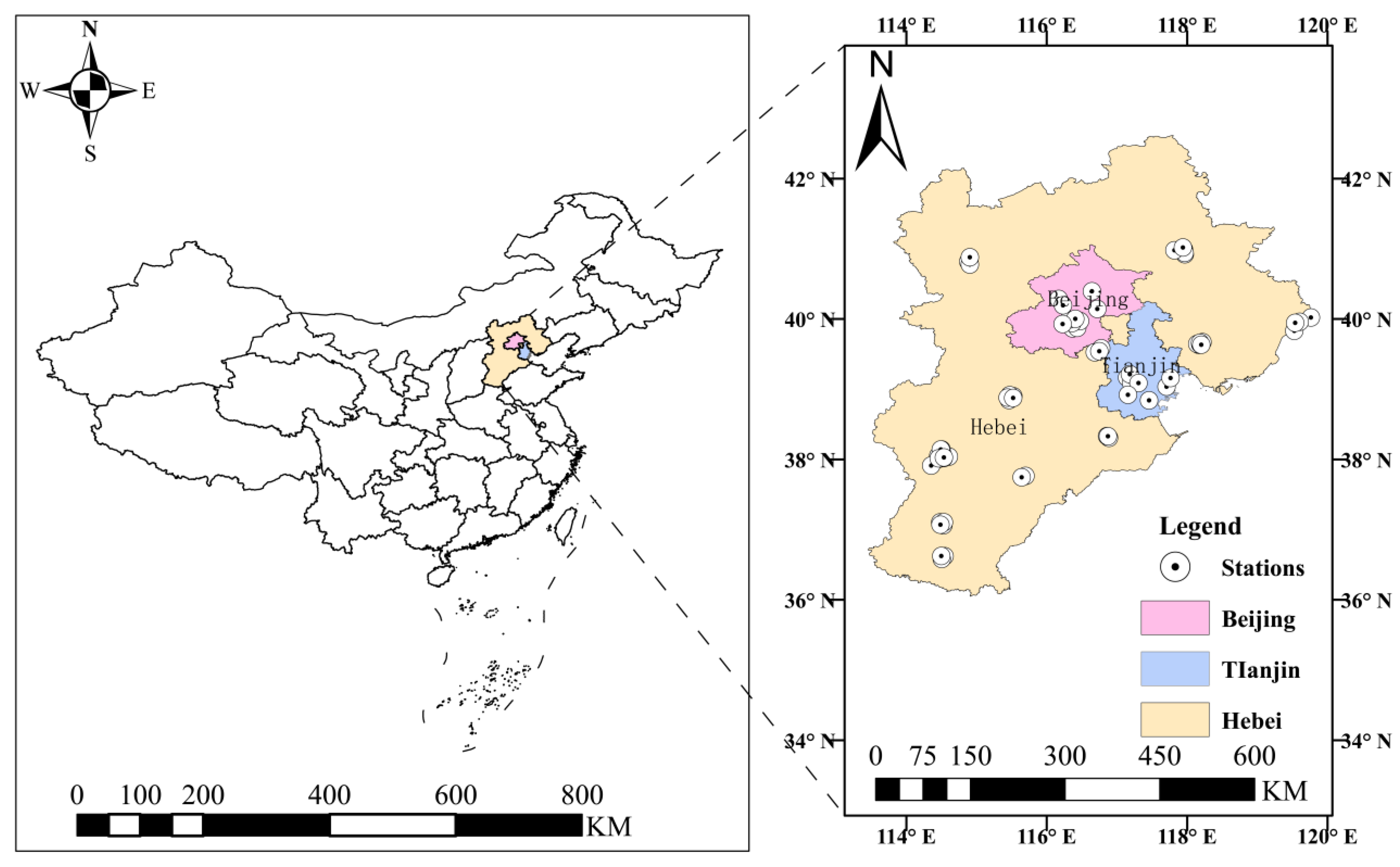
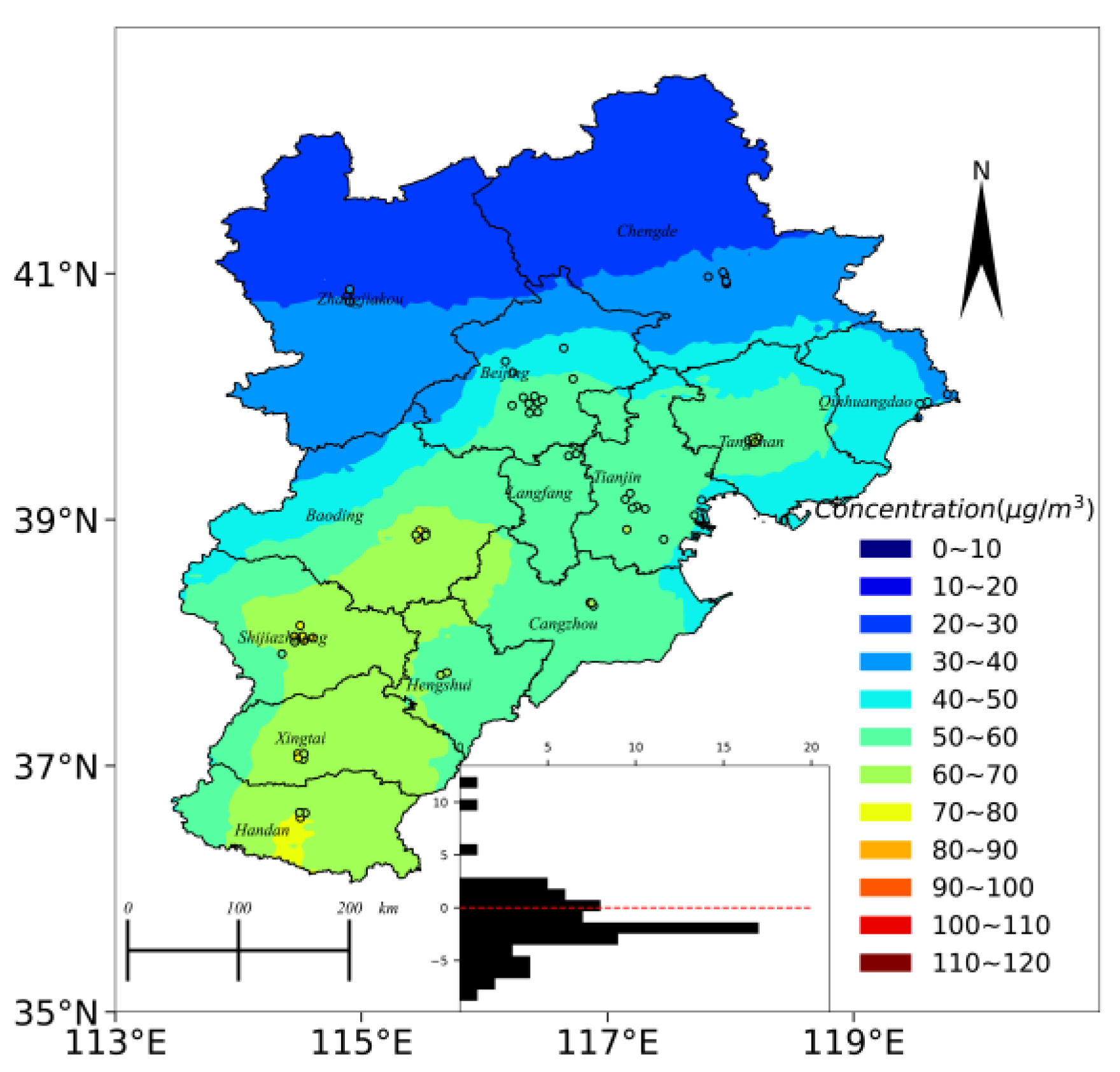
2.1. Study Region

The BTH region in northern China serves as a prominent economic hub. However, the presence of advanced industries and unfavorable environmental conditions, including rising relative humidity, has resulted in consistently poor air quality, posing a severe threat to public health, especially among the region’s 30 million elderly and young populations (please refer to Table S1). Given its economic importance and the affluence of its inhabitants, there is a pressing need to monitor hourly concentrations of PM_2.5 in this region. The location of the BTH region and the distributions of stations in the area are shown in Figure 1.

2.2. Materials

This study collected multi-source data containing meteorological conditions, emission factors, satellite-retrieved products, and additional auxiliary data. To prepare the data for analysis, all selected datasets were pre-processed by resampling (0.05° × 0.05°), clipping, and reprojection (WGS-84, EPSG: 4326). The present study also filtered out any observations with NaN values resulting from a lack of measurements. Furthermore, we investigated the spatiotemporal features of the data, such as latitude, longitude, day of the week, and day of the year, to facilitate our study. Details of all the selected variables that PM_2.5 is dependent on are summarized in Table S2.

2.2.1. Ground-Level Observations

This study acquired hourly air quality data from the China National Environmental Monitoring Center (CNEMC) (https://quotsoft.net/air/, accessed on 13 September 2023) and performed data cleaning procedures, such as removing NaN and continuous repeated values. For this study, we utilized data from 178 monitoring stations spanning a geographic range from 35.0°N to 43.0°N and 112.0°E to 120.0°E, with 12 in Beijing, 9 in Tianjin, 51 in Hebei, and 106 others.

2.2.2. Satellite-Derived PM_2.5 Data

The China High Air Pollutant (CHAP) dataset is a publicly available dataset that provides long-term time series data with high accuracy in China (https://weijing-rs.github.io/product.html, accessed on 10 October 2023). This dataset comprises various contents at daily and hourly levels, including PM₁, PM_2.5, PM₁₀, O₃, NO₂, SO₂, and CO. For this study, we specifically selected Himawari-8-derived PM_2.5 in the BTH region in 2018. Note that these PM_2.5 data still have gaps as no AOD gap-filling method is performed. The hourly data was verified against in-situ observations from CNEMC in China, resulting in a cross-validation coefficient of determination (CV-R²) of 0.85, with a root mean squared error and mean absolute error of 13.62 and 8.49 µg/m³, respectively [28].

2.2.3. Auxiliary Factors

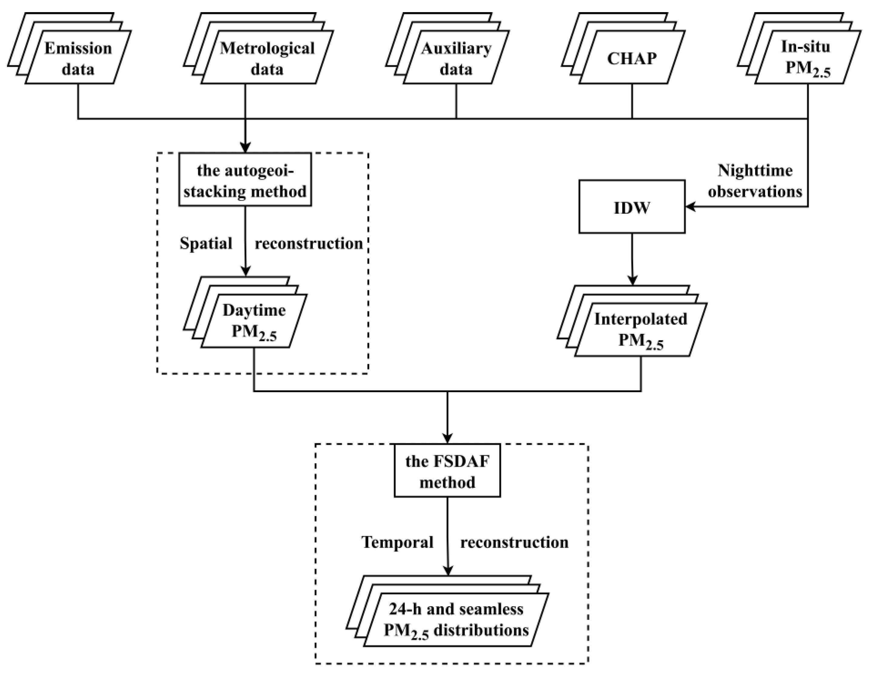
The European Center for Medium Weather Forecasting (ECMWF) Reanalysis v5 (ERA5) dataset is a global atmospheric reanalysis produced by ECMWF. This dataset has been extensively verified in China and found to have the best performance in China against other reanalysis datasets, including the second Modern-Era Retrospective analysis for Research and Applications (MERRA-2), the Japanese 55-year Reanalysis (JRA55), and the NCEP/DOE Reanalysis 2 (NCEP-2)) [29,30,31,32]. Meteorological conditions affecting the accumulation and diffusion of PM_2.5 were selected from the ERA5 dataset, such as boundary-layer height (BLH), total precipitation (TP), and 10 m u/v-component of wind. Details of the selected meteorological factors are provided in Table S2. Using the bilinear interpolation method, the selected independent variables have been resampled to 0.05° × 0.05° (the CHAP’s spatial resolution).

As the manual source affecting air pollution, emissions are essential for PM_2.5 retrieval. In this study, we used the high-resolution air quality reanalysis dataset over China (abbreviated as CAQRA) dataset, which contains emissions data, such as SO₂, NO₂, and CO. This dataset is produced by the chemical data assimilation system (ChemDAS) based on the ensemble Kalman filter and the Nested Air Quality Prediction Modeling System [33]. Emission factors, such as CO and O₃, were added according to the Spearman coefficient.

The chemical composition and other substances that make up PM_2.5 are essential to the atmospheric chemical reactions that can aggravate ambient air pollution [34,35]. For this study, we selected the chemical compositions of the MERRA-2 dataset at the hourly level. MERRA-2 is a comprehensive dataset that integrates multisource data, including ground-based observations, model simulations, and satellite observations. The surface black carbon (BC), organic carbon (OC), dust, sulfate (SO₄), and sea salt (SS) concentrations data were chosen. The PM_2.5 concentrations of MERRA-2 in the BTH region are synthesized by the formula below:

$$\mathrm{P}{\mathrm{M}}_{2.5}={\mathrm{DUST}}_{2.5}+\mathrm{S}{\mathrm{S}}_{2.5}+\mathrm{BC}+1.6\times \mathrm{OC}+1.375\times \mathrm{S}{\mathrm{O}}_4$$

(1)

Arranged from left to right, the symbols in Equation (1) represent the PM_2.5, dust, sea salt, black carbon, organic carbon, and sulfate aerosols data of MERRA-2, all with diameters less or equal to 2.5 µm. The coefficients 1.6 and 1.375 represent China’s representative values, as determined by previous literature [36,37,38,39]. Notably, the nitrate particulate matter predominantly emitted by anthropogenic activities, such as vehicle exhaust and industrial production, is not included in Equation (1) or the MERRA-2 data. This exclusion may lead to biases compared to ground-level observations [40,41].

The Shuttle Radar Topography Mission (SRTM) product is used in this section as it can reflect the fluctuations of the surface. These data are resampled to 0.05° × 0.05°, employing the bilinear interpolation method. Additionally, the spatiotemporal information of datasets (i.e., day of the year, day of the week, longitude, and latitude) is also included as independent variables.

3. Methodology

The main procedure of the proposed framework contains two parts, including a stage called spatial reconstruction that generates spatially full-coverage PM_2.5 during the day based on machine-learning approaches and another stage called temporal reconstruction, which utilizes the FSDAF method to obtain the PM_2.5 distributions of the BTH region. It should be noted that the first stage is replaceable with other machine-learning methods or models to suit specific research needs (i.e., for more robust predictions). The details of both parts are provided in the following sections and the Supplementary Material. The schematic diagram of the proposed framework is illustrated in Figure 2.

3.1. Spatial Reconstruction

For the first stage, the present study employs a previously proposed autogeoi-stacking method [42] as it outperformed single tree-based models such as Random Forest, Gradient Boosting Decision Tree (GBDT), and Extremely Randomized Tree. Due to the advantages of sub-models comprised by the stacking method, model performances are significantly improved. Additionally, the present study utilized an automated feature engineering method that constructs meaningful non-linear features based on multiple mathematic operations, such as logarithmic, sine, and multiplication. Using the autogeoi-stacking approach, the gaps in the CHAP dataset are filled, and spatially seamless PM_2.5 distributions of the BTH region during the day are obtained. However, the proposed method’s complexity may be a limitation for some researchers. In such cases, other robust machine-learning models capable of generating spatially full-coverage PM_2.5 distributions, such as the Light Gradient Boosting Machine (LightGBM) and Extreme Gradient Boosting (Xgboost), may be more suitable. For more detailed descriptions, please refer to Section S1, Refs. [42,43]. The structure of the autogeoi-stacking method can be represented by:

$$\mathrm{P}{\mathrm{M}}_{2.5}=\mathrm{f}\left({\mathrm{f}}_{\mathrm{m}1}(\mathrm{BLH},\mathrm{TP}\dots ,\mathrm{OC},\mathrm{S}{\mathrm{O}}_4,\mathrm{SS}),{\mathrm{f}}_{\mathrm{m}2},\dots {\mathrm{f}}_{\mathrm{m}7}\right)$$

(2)

Equation (2) describes the autogeoi-stacking method, which synthesizes the final estimations of the spatial reconstruction process via stacking through all the predictions of the seven sub-models. The symbol f_m1 represents the process of a well-trained machine-learning method that integrates all the potential factors (e.g., BLH, organic carbon) and estimates the PM_2.5 concentration at each point.

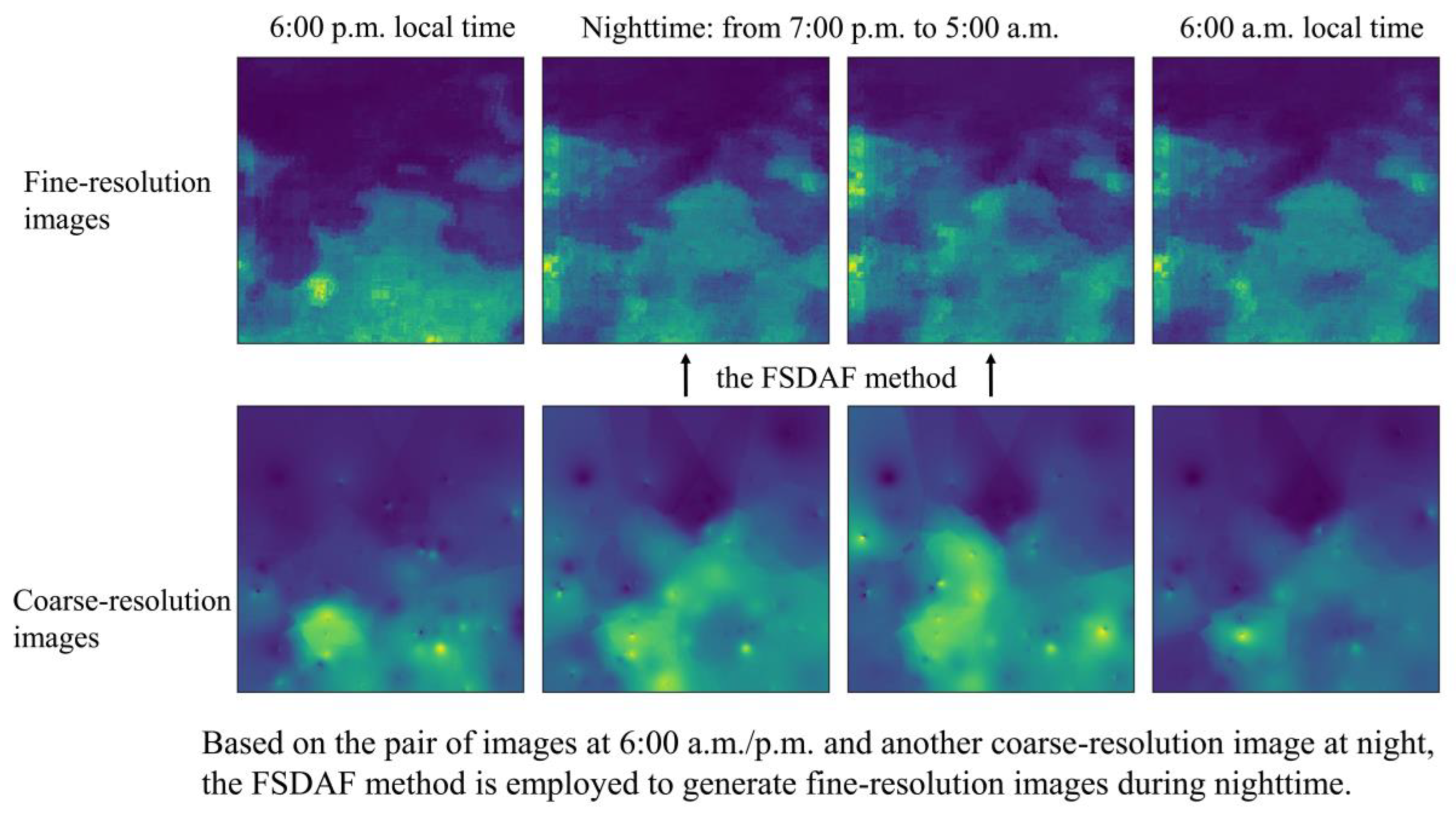
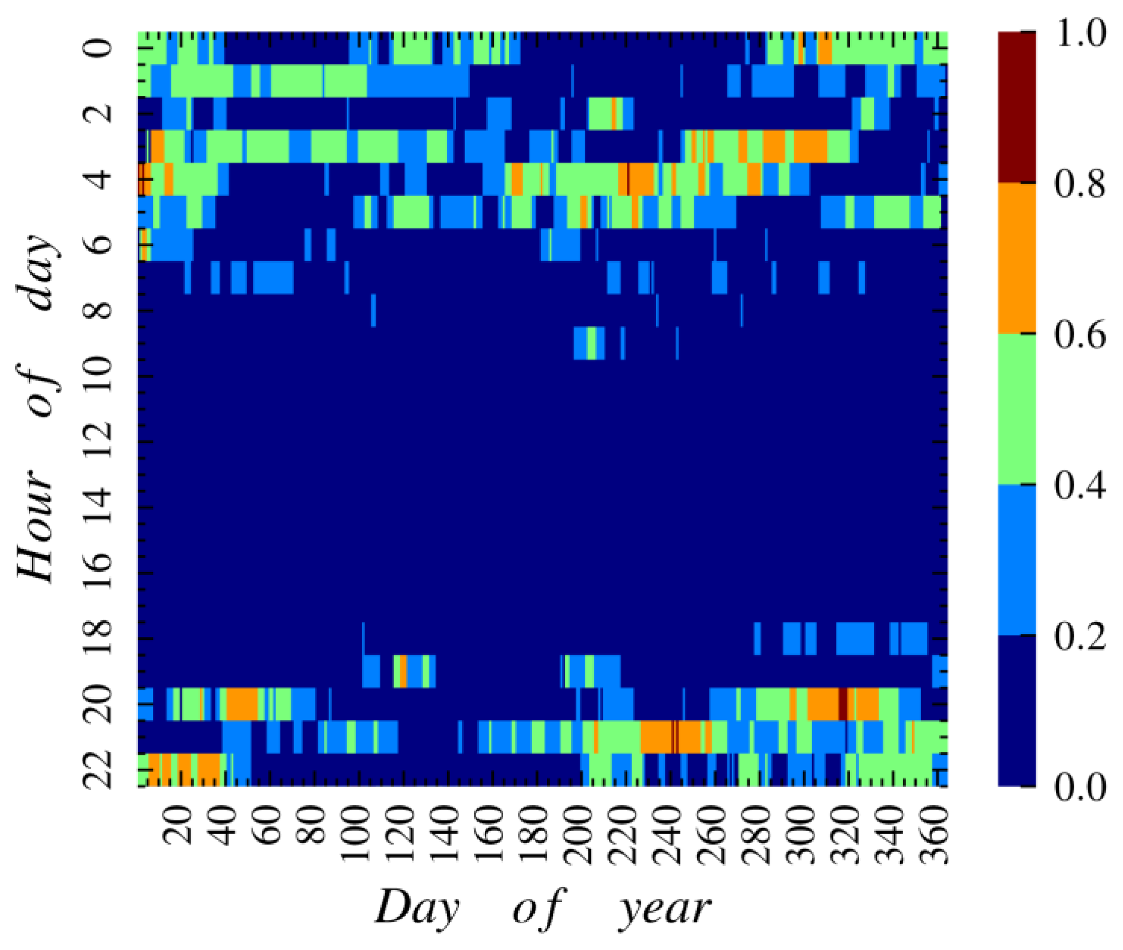
3.2. Temporal Reconstruction

To address the absence of available AOD-derived PM_2.5 products at night, this study employed a robust and efficient data fusion method known as the FSDAF during the second stage. This method, proposed by Ref. [44], has demonstrated its effectiveness in various areas, including the fusion of multiple satellite images and the reconstruction of time series for land surface temperature (LST) and normalized difference vegetation index (NDVI) time series [45,46,47] and was therefore selected for filling the gaps in nighttime PM_2.5 data.

To acquire PM_2.5 distributions during nighttime, a pair of PM_2.5 images (i.e., one fine-resolution and coarse-resolution image) and another coarse-resolution image are necessary. In this study, the coarse-resolution images were interpolated using inverse distance weighted (IDW) interpolation based on ground-level observations during the night (between 19:00 and 7:00, local time). Additionally, this study used images generated in the first stage at 8:00 or 18:00 as the fine-resolution images. Based on the pair of images at 18:00 or 8:00 (depending on the temporal adjacency of the nighttime), FSDAF estimated PM_2.5 distributions using the interpolated images at night. The primary process of temporal reconstruction is illustrated in Figure 3. The main procedures of the FSDAF method are described below: (1) classifying the fine-resolution image at t1 via the K-means method; for a given parameter k, the pixels are divided into k classes; (2) the temporal changes for every class are estimated for the coarse-resolution from t1 to t2; (3) predict the fine-resolution image at t2 using the temporal change at class-level and calculate residuals at each coarse pixels; (4) adopting Thin Plate Spline (TPS) interpolation to predict the fine-resolution image from the coarse-resolution image at t2; (5) distributing the residuals based on TPS prediction; (6) using the information in the neighborhood via the moving window method to obtain the final prediction of the fine-resolution image. The FSDAF method used in the present study can be formulated as:

$$\mathrm{P}{\mathrm{M}}_{\mathrm{t}2}\left({\mathrm{x}}_{\mathrm{ij}},{\mathrm{y}}_{\mathrm{ij}}\right)={\mathrm{PM}}_{\mathrm{t}1}\left({\mathrm{x}}_{\mathrm{ij}},{\mathrm{y}}_{\mathrm{ij}}\right)+\sum _{\mathrm{k}-1}^{\mathrm{n}}{\mathrm{W}}_{\mathrm{k}}\times \mathsf{\Delta }\mathrm{PM}\left({\mathrm{x}}_{\mathrm{k}},{\mathrm{y}}_{\mathrm{k}}\right),$$

(3)

$$\mathsf{\Delta }\mathrm{PM}\left({\mathrm{x}}_{\mathrm{ij}},{\mathrm{y}}_{\mathrm{ij}}\right)={\mathrm{R}}_{\mathrm{high} }\left({\mathrm{x}}_{\mathrm{ij}},{\mathrm{y}}_{\mathrm{ij}}\right)+\mathsf{\Delta }\mathrm{PM}\left(\mathrm{c}\right),$$

(4)

where PM_t2 and PM_t1 represent the PM_2.5 concentrations at t2 and t1 of one point (x_ij,y_ij) with a high resolution, respectively. W_k indicates the calculated weight of points (kth class). $\mathsf{\Delta }\mathrm{PM}$ is the calculated temporal change of points from t1 to t2 of the high-resolution image. In Equation (4), R_high is the residual of points between the high-resolution and coarse-resolution images. $\mathsf{\Delta }\mathrm{PM}\left(\mathrm{c}\right)$ indicates the temporal changes of each classified class via the K-means method.

3.3. Validation

A dataset encompassing all available station data from the BTH region during 2018 was used to validate the proposed framework’s performance. The 10-fold cross-validation method was employed using the sklearn library in Python [48]. Firstly, the dataset was randomly and equally divided into ten chunks. Then, nine of these chunks were utilized to train machine-learning models, while the remaining chunk was reserved for measuring the accuracy and performance of the estimations. After ten repeated aforementioned procedures, the results of three commonly employed evaluation indicators, namely the coefficient of Pearson coefficient (r), determination (R²), root mean squared error (RMSE), and mean absolute error (MAE), were obtained. The formulations for these three indicators are as follows:

$$\begin{gathered} \mathrm{r}=\frac{{\sum }_{i=1}^n\left(X_i-\overline{X}\right)\left(Y_i-\overline{Y}\right)}{\sqrt{{\sum }_{i=1}^n{\left(X_i-\overline{X}\right)}^2}\sqrt{{\sum }_{i=1}^n{\left(Y_i-\overline{Y}\right)}^2}}. \\ {\mathrm{R}}^2=1-\frac{{\sum }_i{\left(X_i-Y_i\right)}^2}{{\sum }_i{\left(X_i-\overline{X}\right)}^2}, \end{gathered}$$

(5)

$$\mathrm{MAE}=\frac{1}{\mathrm{m}}{\sum }_{i=1}^{\mathrm{m}}\left|\left(X_i-Y_i\right)\right|$$

(6)

$$\mathrm{and}\mathrm{RMSE}=\sqrt{\frac{1}{\mathrm{m}}{\sum }_{i=1}^{\mathrm{m}}{\left(X_i-Y_i\right)}^2}$$

(7)

where m is the total number of samples engaging the validation, and $\overline{X} \mathrm{and} \overline{Y} \mathrm{are}$ the mean values of observations and estimations of PM_2.5 concentrations, respectively. $X_i$ and $Y_i$ represent the i-th value of ground-based PM_2.5 observations and estimated PM_2.5 concentrations, respectively.

4. Results

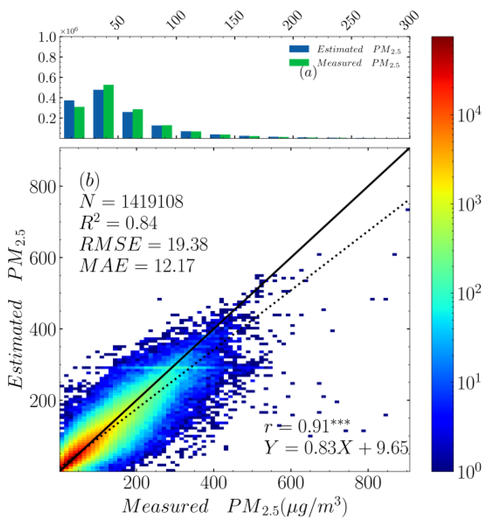
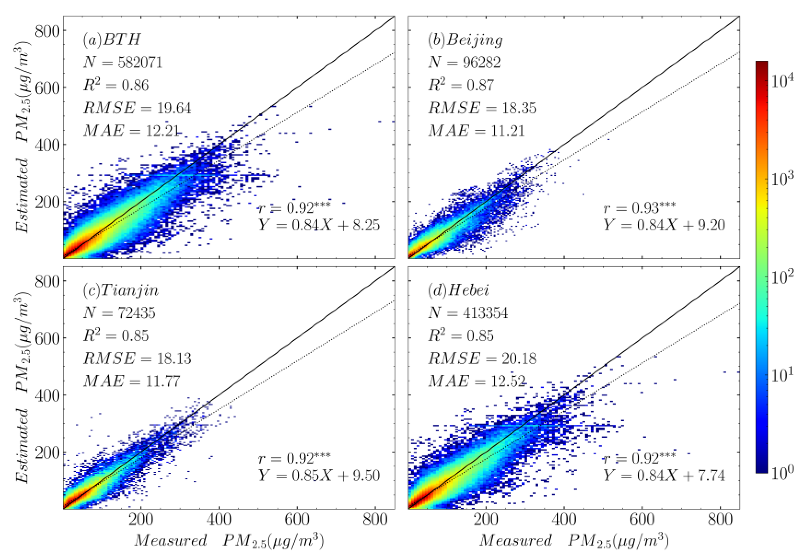
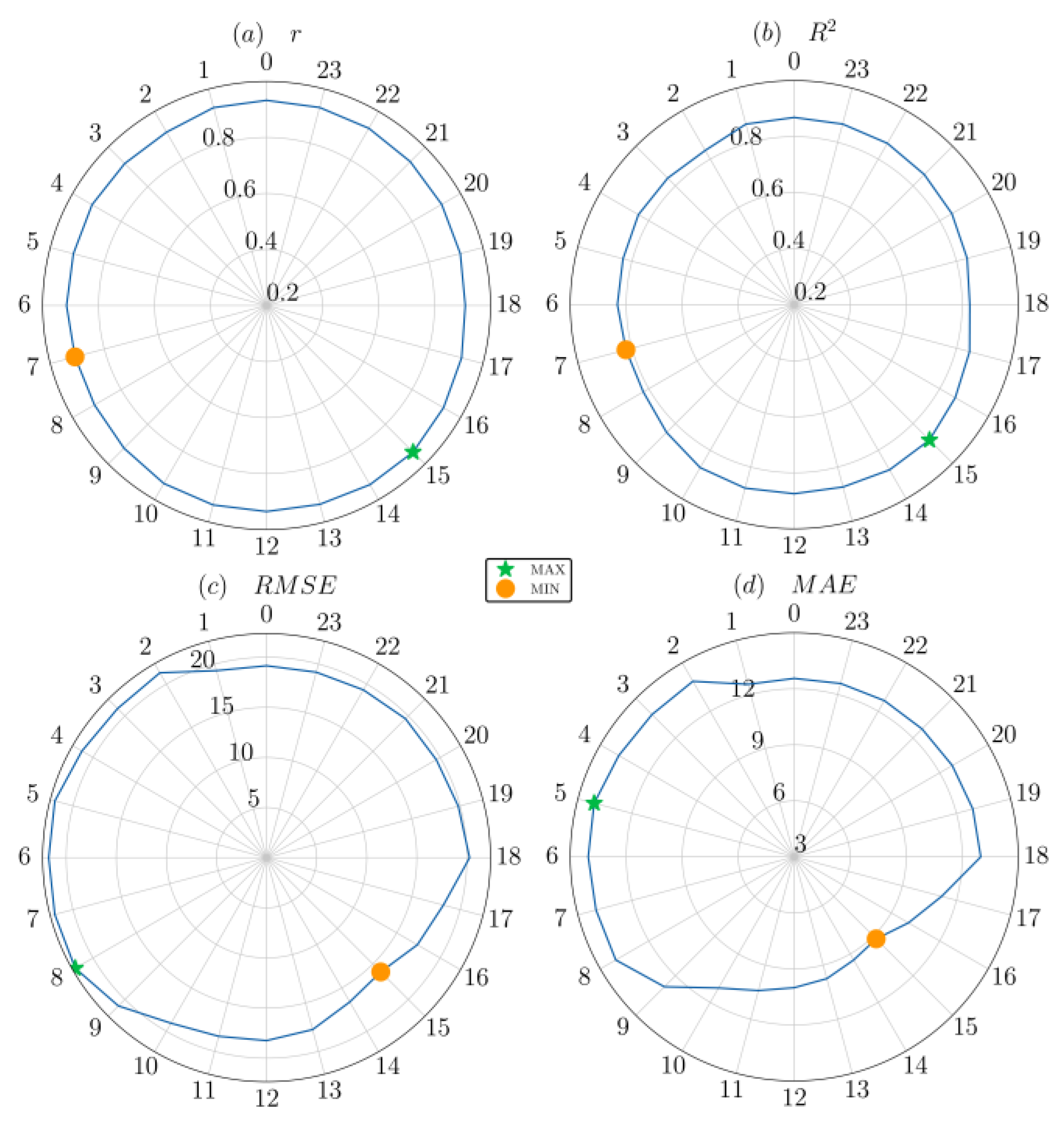
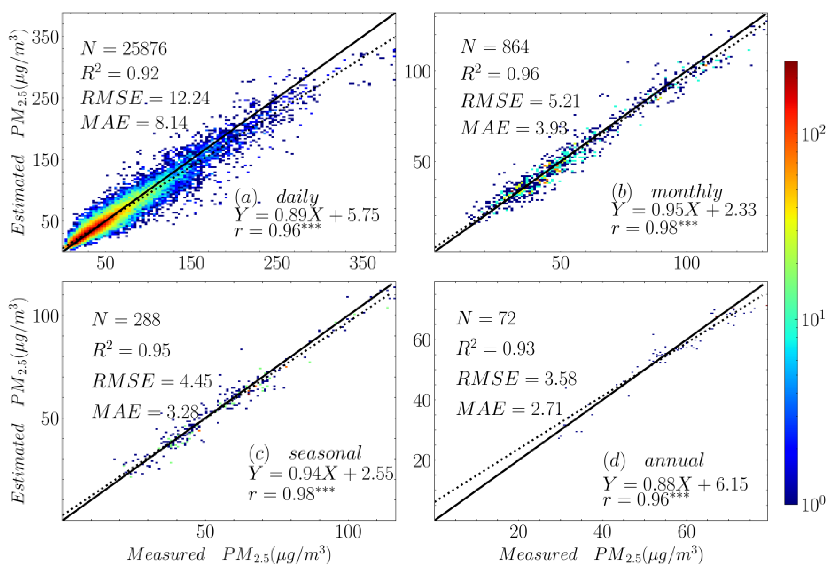
4.1. Model Performances

To validate the performance of the estimated PM_2.5 concentrations, this study employed the 10-fold cross-validation method from the perspectives of all samples, spatial and temporal. The results of all samples were analyzed, and Figure 4a presents a histogram of the estimated and observed PM_2.5, while Figure 4b displays a density scatterplot and performance metrics (r, R², RMSE, and MAE). The estimated and observed PM_2.5 values in Figure 4a were mostly between 0 and 300 µg/m³, with a high density between 0 and 70 µg/m³, accounting for approximately 78.25% and 79.14% for estimated and measured PM_2.5, respectively. These results demonstrate a high level of consistency between the estimations and observations. The robustness of the proposed framework is shown in Figure 4b, with an r of 0.91, an R² of 0.84, an RMSE of 19.38 µg/m³, an MAE of 12.17 µg/m³, and a slope of 0.83.

Spatial-based validation was performed across each sub-region of the BTH region, as shown in Figure 5. The proposed framework demonstrated robust performance within the BTH region, with an r of 0.92, an R² value of 0.86, an RMSE value of 19.64 µg/m³, and an MAE value of 12.21 µg/m³. Furthermore, the framework achieved high accuracy in Beijing (R² = 0.87), Tianjin (R² = 0.85), and Hebei (R² = 0.85). While there are more available samples in Hebei compared to the other two regions, the proposed framework did not perform as effectively in Hebei as it did in the other two areas. This phenomenon may be attributed to the lack of representativeness in the samples, failing to capture the region’s intricate geography characterized by more mountains and terrain fluctuations, along with its poorer air quality. It should be noted that the proposed framework occasionally underestimated high values (i.e., larger than 500 µg/m³), possibly due to a lack of representative data from high-value areas. In such cases, over-sampling and under-sampling techniques could be considered [14,49,50]. Overall, these findings demonstrate the robustness of the proposed framework in the BTH region, with the potential for further improvements in its performance.

Through the seamless dataset in spatial and temporal dimensions, evaluation is made every hour (please refer to Figure 6). The subgraphs have demonstrated the robustness of the proposed framework, with r results consistently exceeding 0.90, R² values consistently surpassing 0.80, RMSE values consistently falling below 22.06 µg/m³, and MAE values consistently remaining under 14.10 µg/m³. Additionally, the range of R² results spans from 0.82 to 0.88, with the highest R² being 0.88 recorded at 3 p.m. (accompanied by RMSE = 16.12 µg/m³ and MAE = 9.21 µg/m³), while the lowest R², at 0.82, was observed at 7 a.m. (associated with RMSE = 21.89 µg/m³ and MAE = 14.00 µg/m³). The range of R² results during the daytime (8:00–18:00, local time) is between 0.82 and 0.88, and the values during the night are between 0.82 and 0.87 (19:00–7:00) (R² values of day and night are 0.83 and 0.82, as depicted in Figure S1). Finally, the results show that the seamless dataset of PM_2.5 documents the spatiotemporal variations well. The proposed framework works robustly, whether during the daytime or the night.

The cross-validation performances of PM_2.5 estimations at different temporal scales are presented in Figure 7. At the daily level (Figure 7a), the proposed framework exhibits robust performance in estimating PM_2.5 concentrations in the BTH region during 2018. The obtained r value of 0.96, R² value of 0.92, and low RMSE and MAE values (12.24 µg/m³ and 8.14 µg/m³, respectively) demonstrate the ability of the framework to capture the daily fluctuations of PM_2.5 concentrations accurately. Notably, the daily synthetic PM_2.5 data frequency is higher than that derived from ground-level observations. At the monthly level (Figure 7b), the estimations of the proposed framework are well-matched with the observed values, as indicated by a slope of 0.95. Overall, the results of the proposed framework consistently demonstrate favorable performance across various temporal scales, ranging from daily to yearly levels, with r values of 0.96–0.98, R² values of 0.92–0.96, RMSE values of 3.58–12.24 µg/m³, MAE values of 2.71–8.14 µg/m³, and slope values of 0.88–0.95, indicating reliable and accurate results. These outcomes support an effective application of the proposed framework in capturing the temporal variations of PM_2.5 concentrations.

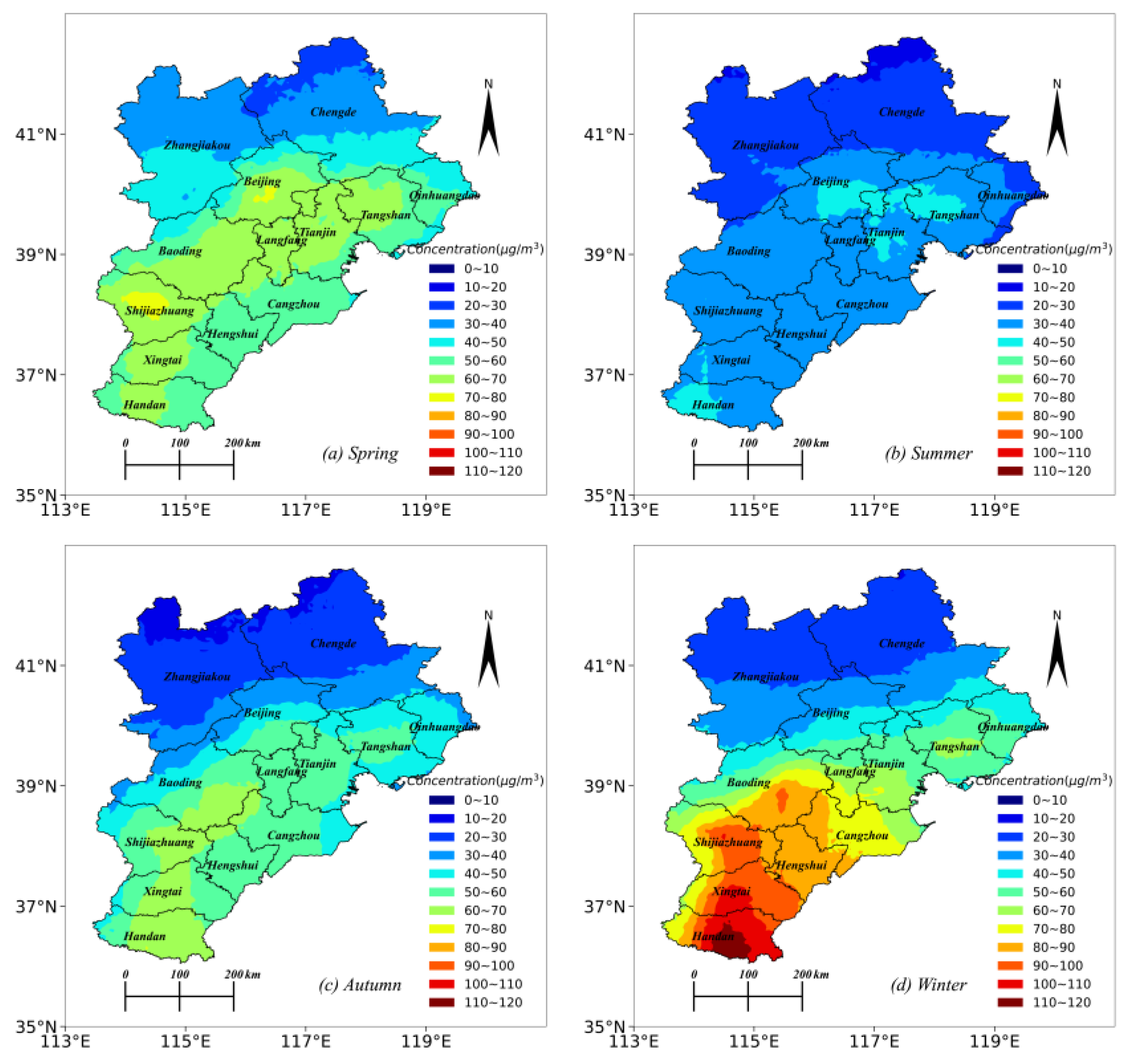
4.2. Spatial Distributions

In this section, this study presents the spatial distributions of the generated data from our study for both seasonal and annual levels, as depicted in Figure 8 and Figure 9. This study compared annual distributions of our data with the two included datasets in this study (MERRA-2, CHAP) and another open gap-free dataset, namely the Long-term Gap-free High-resolution Air Pollutant dataset (LGHAP; details of this dataset are depicted in Section S2) [28,51,52]. Firstly, in Figure 8, this study shows the mean PM_2.5 values for each season in the BTH region. Notably, there is a consistent pattern of higher PM_2.5 levels in the southern areas and lower levels in the northern areas across all seasons. In the spring season, 82.15% of the PM_2.5 values are over 35 µg/m³, with a negligible 0.19% of areas classified as slightly polluted and 17.66% of the region enjoying excellent air quality (as per the national ambient air quality standard for annual PM_2.5 concentration stated in GB 3095-2012; please refer to Table S3). During summer, the mean PM_2.5 values range from 17.57 µg/m³ to 45.02 µg/m³, indicating the lowest pollution level compared to the other seasons. In autumn, the PM_2.5 pollution is severe, ranging from 18.39 µg/m³ to 70.61 µg/m³, and it worsens in winter, with over 26.37% of the southern areas exceeding the 75 µg/m³ threshold and 68.42% of the region’s mean PM_2.5 values being over 35 µg/m³. The seasonal variations in PM_2.5 concentrations are influenced by several factors, including increased BLH and higher water vapor content during the summer and straw-burning activities in autumn, as well as the prevalence of coal heating, reduced airflow, and lower BLH in winter [53,54,55]. The average PM_2.5 concentrations for each season in the BTH region are 51.10 ± 12.34 µg/m³ (mean value ± standard deviation value), 32.36 ± 6.64 µg/m³, 42.32 ± 14.90 µg/m³, and 54.29 ± 25.62 µg/m³, respectively, which slightly differ from the seasonal mean values corresponding to the stations (62.45 ± 11.86 µg/m³, 38.88 ± 7.37 µg/m³, 54.28 ± 13.71 µg/m³, and 68.63 ± 27.65 µg/m³, respectively). In summary, residents living in the southern areas of the BTH region are exposed to higher PM_2.5 levels than those residing in the north. While the pollution is the most severe in winter, followed by spring and autumn, it is relatively lower in summer.

As shown in Figure 9, this study investigated the annual PM_2.5 distributions in both stations and the study area, as well as the residual errors between the estimations and observations. The annual mean concentrations of PM_2.5 in the stations and the BTH region were found to be 56.14 ± 13.18 µg/m³ and 44.97 ± 14.19 µg/m³, respectively, exhibiting a consistent pattern in their distributions. The annual PM_2.5 distributions in the BTH region displayed a similar pattern, which is also apparent in Figure 8. Lower concentrations were observed in the northern areas such as Zhangjiakou (28.91 ± 4.35 µg/m³) and Chengde (28.72 ± 5.89 µg/m³), while higher concentrations were observed in the southern regions such as Shijiazhuang (59.82 ± 5.57 µg/m³), Handan (64.60 ± 5.16 µg/m³), and Xingtai (62.16 ± 3.63 µg/m³). These findings are consistent with previous studies [53,56]. Furthermore, the subgraph reveals that the residual errors are primarily concentrated in the range of −10 µg/m³ to 4 µg/m³, with errors falling within the narrower range of −5 µg/m³ to 5 µg/m³, constituting 85.5% of the total. While the narrower range also demonstrates the robustness of the proposed framework, the distributions of residual errors reveal the underestimations, as indicated by the slope values lower than 1 in Figure 4, Figure 5 and Figure 7.

This study compared our seamless hourly dataset with MERRA-2, CHAP, and LGHAP. Note that LGHAP is a daily and gap-filled dataset with a resolution of 1 km, whereas the other three datasets are resampled to a resolution of 0.05° (comparisons of all datasets are provided in Table S4). The consistency of PM_2.5 distributions (see Figure S2) among all datasets is observable, with a pattern of lower concentrations in the south and higher concentrations in the north. The annual mean values of CHAP (43.91 ± 12.94 µg/m³) and LGHAP (43.67 ± 16.59 µg/m³) and the estimated PM_2.5 (44.97 ± 14.19 µg/m³) in this study were similar. However, MERRA-2 significantly underestimated PM_2.5 (33.19 ± 12.30 µg/m³) due to the lack of nitrate particulate matter. It should be noted that the data presented in Figure 9 and Figure S2d may be over-smoothed, eliminating details in the northern regions, which could be considered the main limitation of the proposed methodology. This could be due to the fact that FSDAF needs to calculate weights based on neighborhood pixels [47,57], or the coarse resolution data generated by IDW does not obtain abundant information of details, which needs further experiments to determine specific reasons.

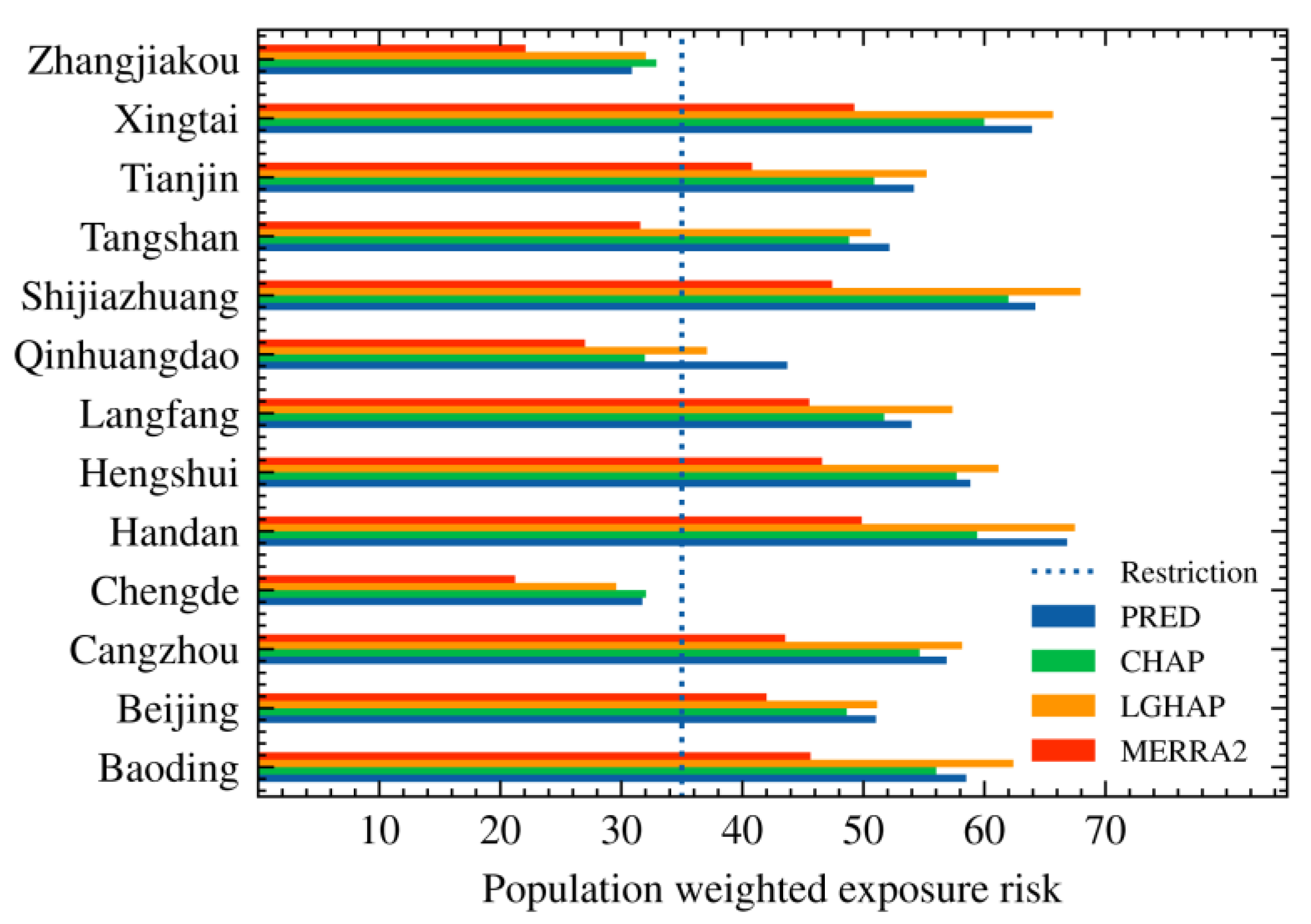
4.3. Particle Exposure Analysis

The adverse effects of PM_2.5 on public health have gained increasing attention, leading to a growing demand for long-term (annual mean) and short-term (24-h) exposure risk assessment [1]. To address this, our study employed the seamless data generated and Landscan as air pollution and demographic data to evaluate annual mean exposure risk using the commonly used population exposure (PWE) metric [58,59]. MERRA-2, CHAP, and the generated data in this study have been resampled to the exact resolution (1 km) of LGHAP and Landscan data. Additionally, we analyzed region exposure risk (RER) at a daily (24-h) level [60]. Details of Landscan, PWE, and RER can be found in Sections S3–S5.

The results show that the PWE metric varied among cities (please refer to

Table 1. PWE, population, and annual mean PM_2.5 of subregions in the BTH region.

	This Study	CHAP	LGHAP	MERRA-2	Population	PM2.5
Beijing	51.04	48.62	51.13	42.00	20,376,165	43.49
Tianjin	54.17	50.88	55.22	40.80	13,480,710	52.83
Hebei	56.24	53.08	57.64	41.78	74,207,325	44.64
BTH	55.00	51.96	56.11	41.69	108,064,754	45.00

, Figure 10 and Figures S3–S7). However, there was high consistency in the distribution of PWE across all datasets, except for MERRA-2, which still underestimated PWE due to the lack of nitrate particulate matter. However, almost all subregions failed to comply with the restriction (the annual values of each city can be seen in Table S5), except for Zhangjiakou (the values of PWE and annual mean are 30.88 µg/m³ and 29.06 µg/m³) and Chengde (31.74 µg/m³ and 29.06 µg/m³), which have excellent air quality attributed to their industrial structural differences led by tourism and more mountains and greenery [61,62]. The generated data were compared with CHAP and LGHAP, and a slight but noticeable difference in PWE was observed, with gap-filled data being more relevant. For instance, the generated data had a better correlation with LGHAP (r = 0.97, R² = 0.91) than with CHAP (r= 0.96, R² = 0.7) (please refer to Figures S8 and S9), possibly due to the poor coverage (32.62%; see Table S4) during the day caused by data gaps and the worsened air pollution during the night than the day (mean values of the night and day are 55.51 µg/m³ and 32.62 µg/m³, respectively; see Figures S10 and S11), which CHAP ignored. These findings suggest that the proposed framework effectively filled the data gaps of PM_2.5, reducing the bias of exposure risk caused by data gaps.

The ambient 24-h exposure risk was evaluated by assessing the RER of the BTH region based on the 24-h restriction (75 µg/m³) of GB3095-2012 (refer to Table S3). As shown in Figure 11, RER fluctuated regularly between 0 and 0.6, with a low frequency of severe RER (i.e., larger than 0.6). During the day, RER constantly varied from 0 to 0.4, while worsening at night, with values ranging from 0 to 0.8. These observations align with the patterns seen in the 24-h distribution of estimated PM_2.5, as illustrated in Figure S12. From midnight to 8 a.m., there was an accumulation of high concentrations (70 µg/m³–80 µg/m³) in the southern area, attributed to the low activity of BLH and other adverse meteorological factors. As the day progressed until noon, despite increased vehicle emissions, the rising BLH led to a reduction in concentrations. Moreover, BLH activity continued to mitigate the concentrations until 5 p.m. However, commencing with the evening peak at 6 p.m. and the subsequent decrease in BLH, PM_2.5 began to accumulate [55,63,64]. Moreover, the occurrence of RER between 0.8 and 1.0 was rare in 2018, indicating that severe pollution sweeping across the BTH region is infrequent. Seasonal variations in RER are observed in Figure S13, with the worst situation occurring in winter, followed by autumn and spring, and the mildest in summer. In summary, RER displays volatility at both hourly and seasonal scales.

5. Discussion

5.1. Overall Evaluation Results

The present study employed a flexible framework to address data gaps in PM_2.5, incorporating the autogeoi-stacking and FSDAF methods. Based on this framework, we filled data gaps in CHAP, which had poor coverage (32.96%) during the day, by reconstructing data during the day and night, resulting in at least three times improved coverage. As a result, this study obtained gap-free data at the hourly level (24-h) based on independent variables. The PM_2.5 estimations in this study were evaluated through sample-based (Figure 4), spatial-based (Figure 5), and temporal-based (Figure 6, Figure 7 and Figure S1) validations. According to the validation of all samples, Figure 4 illustrates a similar pattern in the histogram distributions between the in-situ observations and estimations, demonstrating robust performance with r (0.91), R² (0.84), RMSE (19.38 µg/m³), and MAE (12.17 µg/m³). Figure 5 also demonstrates the robustness of the proposed framework in the BTH region, with r results ranging from 0.92 to 0.93, R² values ranging from 0.85 to 0.87, RMSE values ranging from 18.13 µg/m³ to 20.18 µg/m³, and MAE values ranging from 11.21 µg/m³ to 12.52 µg/m³. The results of temporal-based validation consistently perform well from hourly to annual levels, with r values ranging from 0.91 to 0.98, R² values ranging from 0.82 to 0.96, RMSE values ranging from 3.58 µg/m³ to 21.89 µg/m³, and MAE values ranging from 2.71 µg/m³ to 14.00 µg/m³. However, the density scatterplots (Figure 4, Figure 5, Figure 7 and Figure S1) and the range of slopes of the best-fit lines (0.83–0.94) indicate an increasing underestimation of high-value areas. This underestimation can be attributed to the limited number of representative samples available in areas with values larger than 500 µg/m³, resulting in insufficient information. Therefore, it is crucial to consider under-sampling and over-sampling techniques that maintain a balance between majority (less than 500 µg/m³) and minority (larger than 500 µg/m³) classes [14,49,50].

5.2. Comparison with Related Studies

An essential comparison with relevant studies that have attempted to address data gaps using machine-learning algorithms and interpolation techniques has been conducted [14,24,52]. Firstly, two-stage models, where gap-free AOD is reconstructed and then inverse PM_2.5 is obtained, are compared. For instance, Ref. [16] utilized the multiple imputation method, Ref. [65] employed the inversed variance weights technique, and Ref. [66] adopted the ordinary least square approach. These studies achieved R² values of 0.71 and 0.82 for 2013 and 2014, 0.63–0.86 for 2013–2016 and 0.92 for 2018, respectively. Other gap-filling methods of PM_2.5 are also compared. For example, Ref. [14] fitted the residuals between chemical transport model simulations and ground-level observations and achieved R² values of 0.80–0.88 from 2014 to 2021. Refs. [25,67] utilized multiple sub-models to reconstruct gap-free PM_2.5 with and without AOD, achieving R² values ranging from 0.55 to 0.77 from daily to annual levels and from 0.84 to 0.90 from hourly to daily levels. A summary of all these comparisons is presented in Table S6.

In comparison to these studies, our study demonstrated robust performance, achieving R² values of 0.92, 0.96, and 0.93 at the daily, monthly, and annual levels, respectively (r: 0.91–0.98, RMSE: 3.58 µg/m³–12.24 µg/m³, MAE: 2.71 µg/m³–8.14 µg/m³). Moreover, this study obtained gap-free PM_2.5, whereas some of the aforementioned studies may have been limited by the quality and quantity of available AOD samples [19,23,68]. However, these studies retained the interpretability of AOD and PM_2.5 imputation, whereas our study could not maintain the ability of PM_2.5 imputation. Interpretability can assist other researchers in better understanding black-box modeling and the relationships between selected variables and targets (i.e., PM_2.5 in this study). Therefore, the lack of interpretability in the proposed framework represents a significant drawback. For future work, attention-based, tree-based, and Bayesian-based approaches that can provide variable importance should be taken into consideration [69,70,71,72].

5.3. Uncertainty of the Framework

Based on the analysis of model performance and the comparison with previous literature, the proposed framework exhibited robust performance and significantly reduced the bias in estimated PM_2.5. This could be attributed to several factors. Firstly, by reconstructing 24-h PM_2.5 concentrations in the BTH region for 2018 and improving the coverage at least three times, we mitigated the sampling bias resulting from data gaps to a certain extent. This reduction in bias was achieved by addressing the incomplete data and enhancing the representativeness of the dataset. Secondly, the stacking method employed in the first sub-model of our framework played a crucial role in reducing the uncertainty associated with PM_2.5 estimation. By combining the estimated values from multiple sub-models, the stacking method helped to enhance the accuracy and reliability of the PM_2.5 estimates. This approach has been supported by previous studies [7,69,73]. Further, our framework incorporated prior knowledge from in-situ observations to fill data gaps during the night, which assisted in improving the completeness and accuracy of the PM_2.5 estimates. Given the significant reliance on in-situ observations, particularly at night, future research should take into account the utilization of available coarse-resolution imagery, such as synthetic AOD or PM_2.5 using machine-learning techniques. However, it is also essential to note that due to the low frequency of severe air pollution events in 2018 (as shown in Figure 11), sampling bias emerged, resulting in fewer representative values of high-value areas. Consequently, the proposed framework exhibited underestimation in these areas. This observation aligns with findings from previous studies [24,53,54], highlighting the challenges associated with accurately estimating high PM_2.5 concentration with limited data on air pollution events.

5.4. Differences in Filled and Unfilled Data

To understand the difference between filled and unfilled PM_2.5 data, we conducted a comparison between them, considering annual mean values, distributions, and RER. Overall, consistency was observed among all datasets in terms of these measures. However, the present study calculated PWE and obtained more accurate values than unfilled data for the BTH region (55.00 µg/m³), Beijing (51.04 µg/m³), Tianjin (54.17 µg/m³), and Hebei (56.24 µg/m³). It is worth noting that the calculated PWE in our study differed from CHAP’s estimate, which exhibited a certain degree of underestimation compared to the gap-free data. This underestimation can be attributed to omitting data gaps during the day and night. Our findings regarding PWE suggest that data gaps not only affect the accuracy and coverage of retrieved PM_2.5 data but also introduce additional bias in assessing exposure risk based on these data [14,52]. However, due to the differences in the spatial resolution of LGHAP (1-km), CHAP (0.05°), and this study (0.05°), it is also essential to consider the spatial-resolution-related bias of exposure risk [74,75]. For instance, Ref. [74] investigated the difference between 100-km and 1-km data from 2010 to 2020. They found a 7% underestimation of the long-trend of national PWE and a 1.75% underestimation of the national attributable mortality trend.

Our comparison analysis revealed that filling data gaps in PM_2.5 retrieval led to more accurate PWE values than unfilled data. This underscores the importance of addressing data gaps to improve the accuracy of exposure risk assessments. However, it is also crucial to consider spatial-resolution-related bias when interpreting the results and assessing long-term trends.

5.5. Limitations

Although the proposed framework demonstrated robust performance and effectively highlighted the differences between gap-filled and non-gap-filled data, our study still has several limitations. These limitations include the high dependency of in-situ observations, the lack of interpretability in PM_2.5 imputation, underestimation caused by sampling bias, and spatial-resolution-related bias of exposure risk.

Given the substantial reliance on in-situ observations, at least two approaches should be considered. First, it is imperative to assess the model’s performance when a portion of the site data is intentionally omitted, employing repeated out-of-station verification to evaluate the model’s generalization capabilities. Second, it is crucial to investigate alternative data sources, such as synthetic AOD or PM_2.5 generated through machine-learning techniques, to complement available coarse-resolution imagery.

To address the second limitation, exploring alternative interpretability models such as attention-based, tree-based, and Bayesian-based approaches is recommended. These models can provide insights into the relationships between selected and target variables, enhancing understanding of the underlying mechanisms and improving interpretability.

To mitigate the underestimation caused by sampling bias, future work should consider the application of under-sampling and over-sampling techniques. Techniques such as the Synthetic Minority Over-sampling Technique (SMOTE) can be utilized to balance the representation of different classes and ensure more accurate estimations in high-value areas. By addressing the imbalanced nature of the data, the bias in estimating extreme pollution events can be reduced.

Regarding the spatial-resolution-related bias of exposure risk, incorporating high-resolution data, such as MAIAC AOD, should be considered. Utilizing high-resolution data can provide more detailed and precise information on the spatial distribution of PM_2.5, thereby reducing the bias associated with coarser spatial resolutions.

6. Conclusions

This study employed a flexible framework incorporating the autogeoi-stacking and FSDAF methods to address data gaps in 24-h PM_2.5 based on independent variables. The performance of the proposed framework was robust across sample-based (R²: 0.84), spatial-based (R²: 0.85–0.87), and temporal-based (R²: 0.82–0.96) validations. Analysis of RER and seasonal distributions revealed that estimated PM_2.5 is the most severe in winter, followed by spring and autumn, while it is relatively lower in summer. The same pattern of distributions of PM_2.5 concentrations showed higher levels in the south and lower levels in the north. Furthermore, the comparison between unfilled and gap-free data in this study demonstrated that gap-free data reduced the bias of PWE caused by data gaps and acquired more accurate results (51.04 µg/m³) in the BTH region. Future studies should explore alternative interpretability models, utilize sampling techniques to address bias, and consider incorporating high-resolution data. These steps can improve the accuracy, interpretability, and spatial resolution of PM_2.5 estimation and enhance the assessment of exposure risks.

References

1. World Health Organization. WHO Global Air Quality Guidelines: Particulate Matter (PM2.5 and PM10), Ozone, Nitrogen Dioxide, Sulfur Dioxide and Carbon Monoxide; WHO: Geneva, Switzerland, 2021. [Google Scholar]
2. Badyda, A.J.; Grellier, J.; Dąbrowiecki, P. Ambient PM2.5 Exposure and Mortality Due to Lung Cancer and Cardiopulmonary Diseases in Polish Cities. In Respiratory Treatment and Prevention; Advances in Experimental Medicine and Biology; Pokorski, M., Ed.; Springer International Publishing: Cham, Switzerland, 2016; Volume 944, pp. 9–17. ISBN 978-3-319-44487-1. [Google Scholar]
3. Wang, J.; Yi, X.; Zhang, J.; Wang, Z.; Li, T.; Zheng, Y.; Huang, B.; Zhang, H.; Rajagopalan, S.; Al-Kindi, S.G.; et al. Air Pollution and Cardiovascular Disease. J. Am. Coll. Cardiol. 2018, 72, 2054–2070. [Google Scholar] [CrossRef]
4. Wu, X.; Zhu, B.; Zhou, J.; Bi, Y.; Xu, S.; Zhou, B. The Epidemiological Trends in the Burden of Lung Cancer Attributable to PM2.5 Exposure in China. BMC Public Health 2021, 21, 737. [Google Scholar] [CrossRef]
5. Fang, X.; Zou, B.; Liu, X.; Sternberg, T.; Zhai, L. Satellite-Based Ground PM2.5 Estimation Using Timely Structure Adaptive Modeling. Remote Sens. Environ. 2016, 186, 152–163. [Google Scholar] [CrossRef]
6. She, Q.; Choi, M.; Belle, J.H.; Xiao, Q.; Bi, J.; Huang, K.; Meng, X.; Geng, G.; Kim, J.; He, K.; et al. Satellite-Based Estimation of Hourly PM2.5 Levels during Heavy Winter Pollution Episodes in the Yangtze River Delta, China. Chemosphere 2020, 239, 124678. [Google Scholar] [CrossRef]
7. Li, L. A Robust Deep Learning Approach for Spatiotemporal Estimation of Satellite AOD and PM2.5. Remote Sens. 2020, 12, 264. [Google Scholar] [CrossRef]
8. Li, L.; Girguis, M.; Lurmann, F.; Pavlovic, N.; McClure, C.; Franklin, M.; Wu, J.; Oman, L.D.; Breton, C.; Gilliland, F.; et al. Ensemble-Based Deep Learning for Estimating PM2.5 over California with Multisource Big Data Including Wildfire Smoke. Environ. Int. 2020, 145, 106143. [Google Scholar] [CrossRef]
9. Shin, M.; Kang, Y.; Park, S.; Im, J.; Yoo, C.; Quackenbush, L.J.; Wei, J.; Huang, W.; Li, Z.; Xue, W.; et al. Estimating 1-Km-Resolution PM2.5 Concentrations across China Using the Space-Time Random Forest Approach. Remote Sens. Environ. 2019, 231, 111221. [Google Scholar] [CrossRef]
10. Zhang, Y.; Li, Z.; Wei, Y.; Peng, Z. A Satellite-Derived, Ground-Measurement-Independent Monthly PM2.5 Mass Concentration Dataset over China during 2000–2015. Big Earth Data 2022, 6, 633–649. [Google Scholar] [CrossRef]
11. Lee, C.; Lee, K.; Kim, S.; Yu, J.; Jeong, S.; Yeom, J. Hourly Ground-Level PM2.5 Estimation Using Geostationary Satellite and Reanalysis Data via Deep Learning. Remote Sens. 2021, 13, 2121. [Google Scholar] [CrossRef]
12. Sun, Y.; Xue, Y.; Jiang, X.; Jin, C.; Wu, S.; Zhou, X. Estimation of the PM2.5 and PM10 Mass Concentration over Land from FY-4A Aerosol Optical Depth Data. Water Resour. Res. 2019, 13, 4276. [Google Scholar] [CrossRef]
13. Yan, X.; Zang, Z.; Luo, N.; Jiang, Y.; Li, Z. New Interpretable Deep Learning Model to Monitor Real-Time PM2.5 Concentrations from Satellite Data. Remote Sens. Environ. 2020, 144, 106060. [Google Scholar] [CrossRef]
14. Geng, G.; Xiao, Q.; Liu, S.; Liu, X.; Cheng, J.; Zheng, Y.; Xue, T.; Tong, D.; Zheng, B.; Peng, Y.; et al. Tracking Air Pollution in China: Near Real-Time PM2.5 Retrievals from Multisource Data Fusion. Environ. Sci. Technol. 2021, 55, 12106–12115. [Google Scholar] [CrossRef] [PubMed]
15. Huang, K.; Bi, J.; Meng, X.; Geng, G.; Lyapustin, A.; Lane, K.J.; Gu, D.; Kinney, P.L.; Liu, Y. Estimating Daily PM2.5 Concentrations in New York City at the Neighborhood-Scale: Implications for Integrating Non-Regulatory Measurements. Sci. Total Environ. 2019, 697, 134094. [Google Scholar] [CrossRef]
16. Xiao, Q.; Wang, Y.; Chang, H.H.; Meng, X.; Geng, G.; Lyapustin, A.; Liu, Y. Full-Coverage High-Resolution Daily PM2.5 Estimation Using MAIAC AOD in the Yangtze River Delta of China. Remote Sens. Environ. 2017, 199, 437–446. [Google Scholar] [CrossRef]
17. Xu, J.; Yang, Z.; Han, B.; Yang, W.; Duan, Y.; Fu, Q.; Bai, Z. A Unified Empirical Modeling Approach for Particulate Matter and NO2 in a Coastal City in China. Chemosphere 2022, 299, 134384. [Google Scholar] [CrossRef] [PubMed]
18. Li, T.; Zhang, C.; Shen, H.; Yuan, Q.; Zhang, L. Real-time and Seamless Monitoring of Ground-level PM2.5 Using Satellite Remote Sensing. ISPRS Ann. Photogramm. Remote Sens. Spat. Inf. Sci. 2018, IV–3, 143–147. [Google Scholar] [CrossRef]
19. Wu, J.; Li, T.; Zhang, C.; Cheng, Q.; Shen, H. Hourly PM2.5 Concentration Monitoring with Spatiotemporal Continuity by the Fusion of Satellite and Station Observations. IEEE J. Sel. Top. Appl. Earth Obs. Remote Sens. 2021, 14, 8019–8032. [Google Scholar] [CrossRef]
20. Kloog, I.; Nordio, F.; Coull, B.A.; Schwartz, J. Incorporating Local Land Use Regression And Satellite Aerosol Optical Depth In A Hybrid Model Of Spatiotemporal PM2.5 Exposures In The Mid-Atlantic States. Environ. Sci. Technol. 2012, 46, 11913–11921. [Google Scholar] [CrossRef]
21. Xu, X.; Zhang, C.; Liang, Y. Review of Satellite-Driven Statistical Models PM2.5 Concentration Estimation with Comprehensive Information. Atmos. Environ. 2021, 256, 118302. [Google Scholar] [CrossRef]
22. Zeng, Q.; Zhu, H.; Gao, Y.; Xie, T.; Liu, S.; Chen, L. Estimating Full-Coverage PM2.5 Concentrations Based on Himawari-8 and NAQPMS Data over Sichuan-Chongqing. Appl. Sci. 2022, 12, 7065. [Google Scholar] [CrossRef]
23. Zhang, D.; Du, L.; Wang, W.; Zhu, Q.; Bi, J.; Scovronick, N.; Naidoo, M.; Garland, R.M.; Liu, Y. A Machine Learning Model to Estimate Ambient PM2.5 Concentrations in Industrialized Highveld Region of South Africa. Remote Sens. Environ. 2021, 266, 112713. [Google Scholar] [CrossRef]
24. Li, K.; Bai, K.; Li, Z.; Guo, J.; Chang, N.-B. Synergistic Data Fusion of Multimodal AOD and Air Quality Data for near Real-Time Full Coverage Air Pollution Assessment. J. Environ. Manag. 2022, 302, 114121. [Google Scholar] [CrossRef]
25. Liu, Y.; Li, C.; Liu, D.; Tang, Y.; Seyler, B.C.; Zhou, Z.; Hu, X.; Yang, F.; Zhan, Y. Deriving Hourly Full-Coverage PM2.5 Concentrations across China’s Sichuan Basin by Fusing Multisource Satellite Retrievals: A Machine-Learning Approach. Atmos. Environ. 2022, 271, 118930. [Google Scholar] [CrossRef]
26. Cui, Q.; Zhang, F.; Fu, S.; Wei, X.; Ma, Y.; Wu, K. High Spatiotemporal Resolution PM2.5 Concentration Estimation with Machine Learning Algorithm: A Case Study for Wildfire in California. Remote Sens. 2022, 14, 1635. [Google Scholar] [CrossRef]
27. Wang, W.; He, Q.; Zhang, M.; Zhang, W.; Zhu, H. Full-Coverage 1-Km Estimates and Spatiotemporal Trends of Aerosol Optical Depth over Taiwan from 2003 to 2019. Atmos. Pollut. Res. 2022, 13, 101579. [Google Scholar] [CrossRef]
28. Wei, J.; Li, Z.; Pinker, R.T.; Wang, J.; Sun, L.; Xue, W.; Li, R.; Cribb, M. Himawari-8-Derived Diurnal Variations in Ground-Level PM2.5 Pollution across China Using the Fast Space-Time Light Gradient Boosting Machine (LightGBM). Atmos. Chem. Phys. 2021, 21, 7863–7880. [Google Scholar] [CrossRef]
29. Jiang, H.; Yang, Y.; Bai, Y.; Wang, H. Evaluation of the Total, Direct, and Diffuse Solar Radiations From the ERA5 Reanalysis Data in China. IEEE Geosci. Remote Sens. Lett. 2020, 17, 47–51. [Google Scholar] [CrossRef]
30. Jiang, Q.; Li, W.; Fan, Z.; He, X.; Sun, W.; Chen, S.; Wen, J.; Gao, J.; Wang, J. Evaluation of the ERA5 Reanalysis Precipitation Dataset over Chinese Mainland. J. Hydrol. 2021, 595, 125660. [Google Scholar] [CrossRef]
31. Bao, X.; Zhang, F. How Accurate Are Modern Atmospheric Reanalyses for the Data-Sparse Tibetan Plateau Region? J. Clim. 2019, 32, 7153–7172. [Google Scholar] [CrossRef]
32. Guo, J.; Zhang, J.; Yang, K.; Liao, H.; Zhang, S.; Huang, K.; Lv, Y.; Shao, J.; Yu, T.; Tong, B.; et al. Investigation of Near-Global Daytime Boundary Layer Height Using High-Resolution Radiosondes: First Results and Comparison with ERA5, MERRA-2, JRA-55, and NCEP-2 Reanalyses. Atmos. Chem. Phys. 2021, 21, 17079–17097. [Google Scholar] [CrossRef]
33. Kong, L.; Tang, X.; Zhu, J.; Wang, Z.; Li, J.; Wu, H.; Wu, Q.; Chen, H.; Zhu, L.; Wang, W.; et al. A 6-Year-Long (2013–2018) High-Resolution Air Quality Reanalysis Dataset in China Based on the Assimilation of Surface Observations from CNEMC. Earth Syst. Sci. Data 2021, 13, 529–570. [Google Scholar] [CrossRef]
34. Sun, Y.L.; Wang, Z.F.; Du, W.; Zhang, Q.; Wang, Q.Q.; Fu, P.Q.; Pan, X.L.; Li, J.; Jayne, J.; Worsnop, D.R. Long-Term Real-Time Measurements of Aerosol Particle Composition in Beijing, China: Seasonal Variations, Meteorological Effects, and Source Analysis. Atmos. Chem. Phys. 2015, 15, 10149–10165. [Google Scholar] [CrossRef]
35. Prijith, S.S.; Moorthy, K.K.; Babu, S.N.S.; Satheesh, S.K. Characterization of Particulate Matter and Black Carbon over Bay of Bengal during Summer Monsoon: Results from the OMM Cruise Experiment. Environ. Sci. Pollut. Res. 2018, 25, 33162–33171. [Google Scholar] [CrossRef] [PubMed]
36. Bali, K.; Dey, S.; Ganguly, D. Diurnal Patterns in Ambient PM2.5 Exposure over India Using MERRA-2 Reanalysis Data. Environ. Res. 2021, 248, 118180. [Google Scholar] [CrossRef]
37. Buchard, V.; da Silva, A.M.; Randles, C.A.; Colarco, P.; Ferrare, R.; Hair, J.; Hostetler, C.; Tackett, J.; Winker, D. Evaluation of the Surface PM2.5 in Version 1 of the NASA MERRA Aerosol Reanalysis over the United States. Atmos. Environ. 2016, 125, 100–111. [Google Scholar] [CrossRef]
38. Ma, J.; Xu, J.; Qu, Y.; Cerqueira, V.; Moniz, N.; Soares, C. Evaluation on the Surface PM2.5 Concentration over China Mainland from NASA’s MERRA-2. Atmos. Environ. 2020, 237, 117666. [Google Scholar] [CrossRef]
39. Provençal, S.; Buchard, V.; da Silva, A.M.; Leduc, R.; Barrette, N. Evaluation of PM Surface Concentrations Simulated by Version 1 of NASA’s MERRA Aerosol Reanalysis over Europe. Atmos. Pollut. Res. 2017, 8, 374–382. [Google Scholar] [CrossRef]
40. He, L.; Lin, A.; Chen, X.; Zhou, H.; Zhou, Z.; He, P. Assessment of MERRA-2 Surface PM2.5 over the Yangtze River Basin: Ground-Based Verification, Spatiotemporal Distribution and Meteorological Dependence. Remote Sens. 2019, 11, 460. [Google Scholar] [CrossRef]
41. Song, Z.; Fu, D.; Zhang, X.; Wu, Y.; Xia, X.; He, J.; Han, X.; Zhang, R.; Che, H. Diurnal and Seasonal Variability of PM2.5 and AOD in North China Plain: Comparison of MERRA-2 Products and Ground Measurements. Atmos. Environ. 2018, 191, 70–78. [Google Scholar] [CrossRef]
42. Chu, W.; Zhang, C.; Zhao, Y.; Li, R.; Wu, P. Spatiotemporally Continuous Reconstruction of Retrieved PM2.5 Data Using an Autogeoi-Stacking Model in the Beijing-Tianjin-Hebei Region, China. Remote Sens. 2022, 14, 4432. [Google Scholar] [CrossRef]
43. Horn, F.; Pack, R.; Rieger, M. The Autofeat Python Library for Automated Feature Engineering and Selection. In Proceedings of the Joint European Conference on Machine Learning and Knowledge Discovery in Databases, Würzburg, Germany, 16–20 September 2019; Springer: Berlin/Heidelberg, Germany, 2019; pp. 111–120. [Google Scholar]
44. Zhu, X.; Helmer, E.H.; Gao, F.; Liu, D.; Chen, J.; Lefsky, M.A. A Flexible Spatiotemporal Method for Fusing Satellite Images with Different Resolutions. Remote Sens. Environ. 2016, 172, 165–177. [Google Scholar] [CrossRef]
45. Zhou, J.; Chen, J.; Chen, X.; Zhu, X.; Qiu, Y.; Song, H.; Rao, Y.; Zhang, C.; Cao, X.; Cui, X. Sensitivity of Six Typical Spatiotemporal Fusion Methods to Different Influential Factors: A Comparative Study for a Normalized Difference Vegetation Index Time Series Reconstruction. Remote Sens. Environ. 2021, 252, 112130. [Google Scholar] [CrossRef]
46. Zhu, X.; Zhan, W.; Zhou, J.; Chen, X.; Liang, Z.; Xu, S.; Chen, J. A Novel Framework to Assess All-Round Performances of Spatiotemporal Fusion Models. Remote Sens. Environ. 2022, 274, 113002. [Google Scholar] [CrossRef]
47. Li, Y.; Wu, H.; Li, Z.-L.; Duan, S.; Ni, L. Evaluation of Spatiotemporal Fusion Models in Land Surface Temperature Using Polar-Orbiting and Geostationary Satellite Data. In Proceedings of the IGARSS 2020-2020 IEEE International Geoscience and Remote Sensing Symposium, Waikoloa, HI, USA, 26 September–2 October 2020; IEEE: Waikoloa, HI, USA, 2020; pp. 236–239. [Google Scholar]
48. Rodriguez, J.D.; Perez, A.; Lozano, J.A. Sensitivity Analysis of K-Fold Cross Validation in Prediction Error Estimation. IEEE Trans. Pattern Anal. Mach. Intell. 2010, 32, 569–575. [Google Scholar] [CrossRef] [PubMed]
49. Blagus, R.; Lusa, L. SMOTE for High-Dimensional Class-Imbalanced Data. BMC Bioinform. 2013, 14, 106. [Google Scholar] [CrossRef] [PubMed]
50. Lin, Y.; Mago, N.; Gao, Y.; Li, Y.; Chiang, Y.-Y.; Shahabi, C.; Ambite, J.L.; Chen, J.; Jönsson, P.; Tamura, M.; et al. Estimation of Ground-Level Particulate Matter Concentrations through the Synergistic Use of Satellite Observations and Process-Based Models over South Korea. Atmos. Chem. Phys. 2020, 19, 1097–1113. [Google Scholar] [CrossRef]
51. Randles, C.A.; da Silva, A.M.; Buchard, V.; Colarco, P.R.; Darmenov, A.; Govindaraju, R.; Smirnov, A.; Holben, B.; Ferrare, R.; Hair, J.; et al. The MERRA-2 Aerosol Reanalysis, 1980 Onward. Part I: System Description and Data Assimilation Evaluation. J. Clim. 2017, 30, 6823–6850. [Google Scholar] [CrossRef]
52. Bai, K.; Li, K.; Ma, M.; Li, K.; Li, Z.; Guo, J.; Chang, N.-B.; Tan, Z.; Han, D. LGHAP: The Long-Term Gap-Free High-Resolution Air Pollutant Concentration Dataset, Derived via Tensor-Flow-Based Multimodal Data Fusion. Earth Syst. Sci. Data 2022, 14, 907–927. [Google Scholar] [CrossRef]
53. Ding, Y.; Chen, Z.; Lu, W.; Wang, X. A CatBoost Approach with Wavelet Decomposition to Improve Satellite-Derived High-Resolution PM2.5 Estimates in Beijing-Tianjin-Hebei. Atmos. Environ. 2021, 249, 118212. [Google Scholar] [CrossRef]
54. Liu, N.; Li, S.; Zhang, F. Multi-Scale Spatiotemporal Variations and Drivers of PM2.5 in Beijing-Tianjin-Hebei from 2015 to 2020. Atmosphere 2022, 13, 1993. [Google Scholar] [CrossRef]
55. Xiao, Q.; Zheng, Y.; Geng, G.; Chen, C.; Huang, X.; Che, H.; Zhang, X.; He, K.; Zhang, Q. Separating Emission and Meteorological Contributions to Long-Term PM2.5; Trends over Eastern China during 2000–2018. Atmos. Chem. Phys. 2021, 21, 9475–9496. [Google Scholar] [CrossRef]
56. Wang, L.; Xiong, Q.; Wu, G.; Gautam, A.; Jiang, J.; Liu, S.; Zhao, W.; Guan, H. Spatio-Temporal Variation Characteristics of PM2.5 in the Beijing–Tianjin–Hebei Region, China, from 2013 to 2018. Int. J. Environ. Res. Public Health 2019, 16, 4276. [Google Scholar] [CrossRef] [PubMed]
57. Ma, Y.; Wei, J.; Huang, X. Integration of One-Pair Spatiotemporal Fusion with Moment Decomposition for Better Stability. Front. Environ. Sci. 2021, 9, 14. [Google Scholar] [CrossRef]
58. Abdul Shakor, A.S.; Pahrol, M.A.; Mazeli, M.I. Effects of Population Weighting on PM10 Concentration Estimation. J. Environ. Public Health 2020, 2020, 1561823. [Google Scholar] [CrossRef]
59. Aunan, K.; Ma, Q.; Lund, M.T.; Wang, S. Population-Weighted Exposure to PM2.5 Pollution in China: An Integrated Approach. Environ. Int. 2018, 120, 111–120. [Google Scholar] [CrossRef] [PubMed]
60. Song, J.; Li, C.; Liu, M.; Hu, Y.; Wu, W. Spatiotemporal Distribution Patterns and Exposure Risks of PM2.5 Pollution in China. Remote Sens. 2022, 14, 3173. [Google Scholar] [CrossRef]
61. He, Q.; Huang, B.; Chen, M.; Guo, S.; Hu, M.; Zhang, X. The Spatiotemporal Evolution of Population Exposure to PM2.5 within the Beijing-Tianjin-Hebei Urban Agglomeration, China. J. Clean. Prod. 2020, 265, 121708. [Google Scholar] [CrossRef]
62. Li, Q.; Li, X.; Li, H. Factors Influencing PM2.5 Concentrations in the Beijing–Tianjin–Hebei Urban Agglomeration Using a Geographical and Temporal Weighted Regression Model. Atmosphere 2022, 13, 407. [Google Scholar] [CrossRef]
63. Suriya; Natsagdorj, N.; Aorigele; Zhou, H. Sachurila Spatiotemporal Variation in Air Pollution Characteristics and Influencing Factors in Ulaanbaatar from 2016 to 2019. Atmosphere 2017, 13, 990. [Google Scholar] [CrossRef]
64. Zhai, S.; Jacob, D.J.; Wang, X.; Shen, L.; Li, K.; Zhang, Y.; Gui, K.; Zhao, T.; Liao, H. Fine Particulate Matter (PM2.5) Trends in China, 2013–2018: Separating Contributions from Anthropogenic Emissions and Meteorology. Atmos. Chem. Phys. 2019, 19, 11031–11041. [Google Scholar] [CrossRef]
65. Hua, Z.; Sun, W.; Yang, G.; Du, Q. A Full-Coverage Daily Average PM2.5 Retrieval Method with Two-Stage IVW Fused MODIS C6 AOD and Two-Stage GAM Model. Remote Sens. 2019, 11, 1558. [Google Scholar] [CrossRef]
66. Jing, Y.; Pan, L.; Sun, Y. Estimating PM2.5 Concentrations in a Central Region of China Using a Three-Stage Model. Int. J. Digit. Earth 2023, 16, 578–592. [Google Scholar] [CrossRef]
67. Xue, T.; Zheng, Y.; Tong, D.; Zheng, B.; Li, X.; Zhu, T.; Zhang, Q. Spatiotemporal Continuous Estimates of PM2.5 Concentrations in China, 2000–2016: A Machine Learning Method with Inputs from Satellites, Chemical Transport Model, and Ground Observations. Environ. Int. 2019, 123, 345–357. [Google Scholar] [CrossRef] [PubMed]
68. Sun, J.; Gong, J.; Zhou, J. Estimating Hourly PM2.5 Concentrations in Beijing with Satellite Aerosol Optical Depth and a Random Forest Approach. Sci. Total Environ. 2021, 762, 144502. [Google Scholar] [CrossRef]
69. Chen, J.; Yin, J.; Zang, L.; Zhang, T.; Zhao, M. Stacking Machine Learning Model for Estimating Hourly PM2.5 in China Based on Himawari 8 Aerosol Optical Depth Data. Sci. Total Environ. 2019, 697, 134021. [Google Scholar] [CrossRef]
70. Fu, D.; Song, Z.; Zhang, X.; Xia, X.; Wang, J.; Che, H.; Wu, H.; Tang, X.; Zhang, J.; Duan, M. Mitigating MODIS AOD Non-Random Sampling Error on Surface PM2.5 Estimates by a Combined Use of Bayesian Maximum Entropy Method and Linear Mixed-Effects Model. Atmos. Pollut. Res. 2020, 11, 482–490. [Google Scholar] [CrossRef]
71. Wang, Z.; Hu, B.; Huang, B.; Ma, Z.; Biswas, A.; Jiang, Y.; Shi, Z. Predicting Annual PM2.5 in Mainland China from 2014 to 2020 Using Multi Temporal Satellite Product: An Improved Deep Learning Approach with Spatial Generalization Ability. Nat. Methods 2022, 187, 141–158. [Google Scholar] [CrossRef]
72. Zhang, J.; Li, D.; Xia, Y.; Liao, Q. Bayesian Aerosol Retrieval-Based PM2.5 Estimation through Hierarchical Gaussian Process Models. Mathematics 2022, 10, 2878. [Google Scholar] [CrossRef]
73. Zhang, A.; Fu, T.; Feng, X.; Guo, J.; Liu, C.; Chen, J.; Mo, J.; Zhang, X.; Wang, X.; Wu, W.; et al. Deep Learning-Based Ensemble Forecasts and Predictability Assessments for Surface Ozone Pollution. Geophys. Res. Lett. 2023, 50, e2022GL102611. [Google Scholar] [CrossRef]
74. Bai, H.; Wu, H.; Gao, W.; Wang, S.; Cao, Y. Influence of Spatial Resolution of PM2.5 Concentrations and Population on Health Impact Assessment from 2010 to 2020 in China. Environ. Pollut. 2023, 326, 121505. [Google Scholar] [CrossRef]
75. Aburas, M.M.; Ahamad, M.S.S.; Omar, N.Q.; Liu, T.; Wang, C.; Wang, Y.; Huang, L.; Li, J.; Xie, F.; Zhang, J.; et al. Impacts of Model Resolution on Predictions of Air Quality and Associated Health Exposure in Nanjing, China. Chemosphere 2020, 249, 126515. [Google Scholar] [CrossRef]
76. Kaul, A.; Maheshwary, S.; Pudi, V. AutoLearn—Automated Feature Generation and Selection. In Proceedings of the 2017 IEEE International Conference on Data Mining (ICDM), New Orleans, LA, USA, 18–21 November 2017; pp. 217–226. [Google Scholar]
77. Wu, D.; Liu, W.; Fang, B.; Chen, L.; Zang, Y.; Zhao, L.; Wang, S.; Wang, C.; Marcato, J.; Li, J.; et al. Automated Feature Engineering Improves Prediction of Protein–Protein Interactions. Amino Acids 2019, 51, 1187–1200. [Google Scholar] [CrossRef]
78. Zheng, Z.; Fiore, A.M.; Westervelt, D.M.; Milly, G.P.; Goldsmith, J.; Karambelas, A.; Curci, G.; Randles, C.A.; Paiva, A.R.; Wang, C.; et al. Automated Machine Learning to Evaluate the Information Content of Tropospheric Trace Gas Columns for Fine Particle Estimates Over India: A Modeling Testbed. J. Adv. Model. Earth Syst. 2023, 15. [Google Scholar] [CrossRef]
79. Džeroski, S.; Ženko, B. Is Combining Classifiers with Stacking Better than Selecting the Best One? Mach. Learn. 2004, 54, 255–273. [Google Scholar] [CrossRef]
80. Dobson, J.; Brlght, E.A.; Coleman, P.R.; Durfee, R.C.; Worley, B.A. LandScan: A Global Population Database for Estimating Populations at Risk. In Remotely-Sensed Cities; Mesev, V., Ed.; CRC Press: Boca Raton, FL, USA, 2003; pp. 301–314. ISBN 978-0-429-18116-0. [Google Scholar]
Figure 1. Location of the BTH region and distribution of the stations.
Remotesensing 15 04973 g001
Figure 2. Study flowchart.
Remotesensing 15 04973 g002
Figure 3. The main procedure of temporal reconstruction. PM2.5 concentrations are increasing with the color changing from blue to green.
Remotesensing 15 04973 g003
Figure 4. Histogram plot and density scatterplot of available estimations and in-situ observations are illustrated in (a) and (b), respectively. The number of samples (N) and model performance (r, R2, RMSE, and MAE) are also provided. The *** indicates that the trends are significant at the 99.9% (p < 0.001) confidence level. The units of RMSE and MAE are µg/m3.
Remotesensing 15 04973 g004
Figure 5. Density scatterplots of the BTH region and each sub-region:(a) BTH; (b) Beijing; (c) Tianjin; (d) Hebei. Dashed and solid lines denote the 1:1 and best-fit lines from linear regression. The *** indicates that the trends are significant at the 99.9% (p < 0.001) confidence level.
Remotesensing 15 04973 g005
Figure 6. Radar charts describe the cross-validation results of the proposed framework every hour: (a) r, (b) R2, (c) RMSE, (d) MAE.
Remotesensing 15 04973 g006
Figure 7. Density scatterplots of results of PM2.5 estimates (µg/m3) at (a) daily, (b) monthly, (c) seasonal, and (d) annual levels. The dashed and solid lines denote 1:1 and best-fit lines from linear regression, respectively. The *** indicates that the trends are significant at the 99.9% (p < 0.001) confidence level.
Remotesensing 15 04973 g007
Figure 8. Seasonal average PM2.5 concentrations in the BTH region during 2018. (a): spring, March to May; (b) summer: June to August; (c) autumn: September to November; (d) winter: December to February.
Remotesensing 15 04973 g008
Figure 9. Annual mean values of stations in the BTH region; the subgraph is the distribution of residual errors between the estimated values and observations at these stations.
Remotesensing 15 04973 g009
Figure 10. PWE of subregions at the city level of the BTH region. The dashed line denotes the restriction of annual mean PM2.5 (35 µg/m3) according to GB3095-2012.
Remotesensing 15 04973 g010
Figure 11. RER of the BTH region of each hour in 2018 based on the restriction of 24-h PM2.5 (75 µg/m3) of GB3095-2012.
Remotesensing 15 04973 g011