
Energy-Efficient and High-Performance Ship Classification Strategy Based on Siamese Spiking Neural Network in Dual-Polarized SAR Images
1
School of Electronics and Communication Engineering, Shenzhen Campus of Sun Yat-Sen University, Shenzhen 518107, China
2
Institute of Remote Sensing Satellite, China Academy of Space Technology, Beijing 100094, China
*
Author to whom correspondence should be addressed.
Remote Sens. 2023, 15(20), 4966; https://doi.org/10.3390/rs15204966
Submission received: 30 August 2023
/
Revised: 30 September 2023
/
Accepted: 9 October 2023
/
Published: 14 October 2023
(This article belongs to the Special Issue Radar Signal Processing and Imaging for Ocean Remote Sensing)
Abstract
:Ship classification using the synthetic aperture radar (SAR) images has a significant role in remote sensing applications. Aiming at the problems of excessive model parameters numbers and high energy consumption in the traditional deep learning methods for the SAR ship classification, this paper provides an energy-efficient SAR ship classification paradigm that combines spiking neural networks (SNNs) with Siamese network architecture, for the first time in the field of SAR ship classification, which is called the Siam-SpikingShipCLSNet. It combines the advantage of SNNs in energy consumption and the advantage of the idea in performances that use the Siamese neuron network to fuse the features from dual-polarized SAR images. Additionally, we migrated the feature fusion strategy from CNN-based Siamese neural networks to the SNN domain and analyzed the effects of various spiking feature fusion methods on the Siamese SNN. Finally, an end-to-end error backpropagation optimization method based on the surrogate gradient has been adopted to train this model. Experimental results tested on the OpenSARShip2.0 dataset have demonstrated the correctness and effectiveness of the proposed SAR ship classification strategy, which has the advantages of the higher accuracy, fewer parameters and lower energy consumption compared with the mainstream deep learning method of the SAR ship classification.

1. Introduction
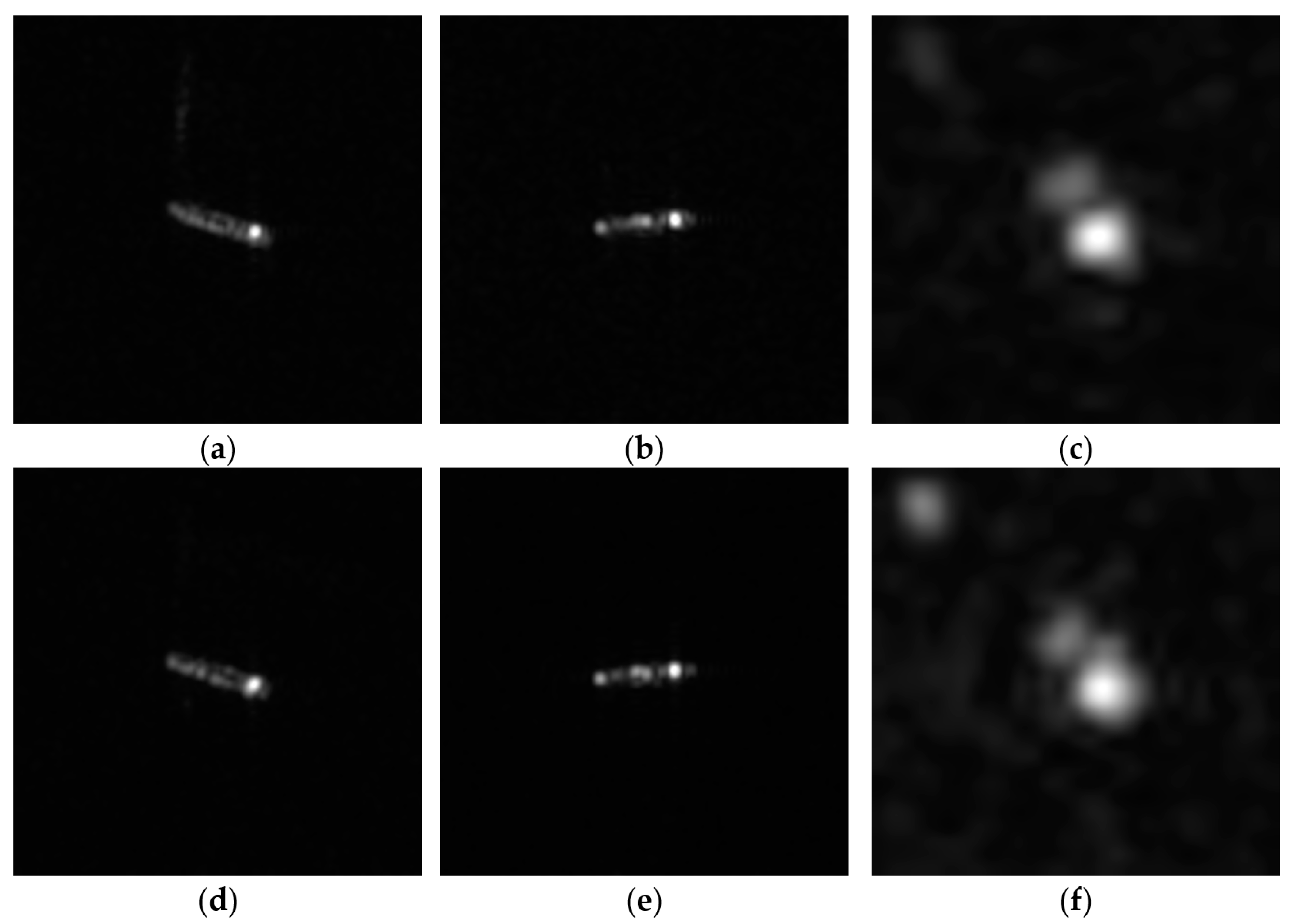
Nowadays, synthetic aperture radar (SAR) systems play an important role in the different application of remote sensing, geosciences, reconnaissance, and surveillance, which have gained the wider attention in the military and civilian fields [1,2,3,4,5]. Ship target recognition and classification using SAR images has significant value in ocean remote sensing applications, since it is able to assist national departments in managing marine ships, as well as the monitoring of marine resource extraction [6,7]. However, because the SAR imaging method mainly relies on the target scattering characteristics, electromagnetic waveforms, and imaging algorithms, the ship targets in the SAR images usually do not have the rich detailed information, and the differences between the different types of ship targets are not significant [7]. Therefore, ship target recognition and classification in the SAR images pose the great challenges. Figure 1 displays some examples of the ship targets in the public SAR image dataset, i.e., the OpenSARShip2.0 dataset [8].
The traditional SAR ship classification method usually achieves the goal of classifying the SAR ships by manually designing the features (such as the geometric structure features, electromagnetic scattering features, transform domain features, local invariant features), but the generalization ability of the traditional SAR ship classification method is usually weak [9,10]. With the development of the deep learning (DL) technology, the artificial neural network (ANN) is gradually replacing the traditional SAR target classification method and becoming the mainstream choice for SAR ship classification [10]. However, due to the lack of the significant feature differences between the SAR ship classes, severe imbalance class distribution of the SAR ships, and a small number of the SAR ship images, SAR ship classification based on the DL also faces the significant challenges. Thus, directly applying the classical image classification networks for the SAR ship classification often results in poor performance. Generally, the SAR image has different polarization modes and data forms in the different domains, thus some researchers are gradually shifting their perspective to fusing the image data from the different sources to improve the performance of the SAR ship classification, such as fusing the SAR ship image data with the different polarization modes [11]. As shown in [12,13,14,15], Siamese network architecture has been used for the information fusion of the multi-polarized SAR ship images to improve the network performance. Reference [12] uses an information fusion method of the element-by-element multiplication, while references [13,14] propose the Bernoulli pooling and grouping Bernoulli pooling methods, respectively, to fuse the information in the SAR images with different polarization methods. In [15], the cross-attention mechanism is applied to fuse the multi-polarized information and enhance the network attention to the key features. In [16], a squeeze-and-excitation Laplacian pyramid network with the dual-polarization feature fusion (SE-LPN-DPFF) for the ship classification in SAR images has been proposed, which reveals the state-of-the-art SAR ship classification performance. In addition, the SAR ship classification method also can use the traditional feature extraction operators to enhance the features of the SAR ships, and then integrates and utilizes the feature learning ability of the neural networks to achieve the better performance. The HOG-ShipCLSNet model has been proposed in [17], even though the neural networks have a strong feature extraction capability, the traditional manually designed features should be utilized to improve the classification accuracy. This model performs the global attention mechanism operations on the features at different levels, and then feeds each level of the feature into the classifier, averaging the results of each classifier. At the same time, the features extracted by the HOG operator are subjected to the principal component analysis, and finally sent to the final classifier to obtain the final classification result. Based on the same idea, the MSHOG operator has been proposed in [18], which can extract the SAR ship features and integrate them into neural networks.
On the other hand, with the rapid development of DL technology, the computing power of the DL model is greatly improved, while it also results in great energy consumption. Nowadays, a serious problem in the artificial intelligence (AI) field is that the training process of DL models is expensive, which will become more and more serious when the computing power of DL models increases. The increase in the energy consumption of ANN computing costs is first attributed to the emergence of the increasingly complex ANN model. In 2018, the natural language processing model BERT [19] released by Google had a parameter count of 340 M. In 2021, the released Switch Transformer [20] had a parameter count of 1.6 × 10⁷ M. In 2023, the latest multimodal large model GPT-4 released by OpenAI caused a huge global response. Although its parameter quantity has not been announced, the industry insiders speculate that it should be equivalent to the parameter quantity of GPT-3 (1.75 × 10⁶ M) [21]. Huge ANN models typically require a significant amount of computing power, and then the high computational costs bring about a sharp increase in energy consumption, which makes it difficult for embedded application platforms with limited energy resources to apply such models. However, designing a network model typically requires repeated adjustments and training, thereby doubling energy consumption.
Although the traditional ANN has made breakthroughs in multiple tasks, the energy consumption issue caused by the cost of the ANN computing makes it difficult to deploy with some resource limited devices and applications. To address this issue, the third-generation ANN called the spiking neural network (SNN) is proposed [22]. SNNs are based on a brain-like computing framework, using spiking neurons as the basic computing unit and transmitting the information through the sparse spiking sequences, which is called a new-generation of green AI technology with lower energy consumption that can run on neural chip devices. Inspired by the operating mechanism of biological neurons, the main core idea of the SNN is to simulate the process of information encoding and transmission between biological neurons using spiking sequences and spiking functions. SNNs can more accurately simulate information expression and the processing process of the human brain, being a brain-like computing model with high biological plasticity, event-driven characteristics, and lower energy consumption [23]. Currently, SNN research is mainly focused on the computer vision field using optical images as carriers. Inspired by histogram clustering, Buhmann et al. [24] first proposed the SNN model based on integrate and fire (IF) neurons, which encodes the image segmentation results with spiking emission frequency. Based on the Time to First Spike encoding strategy, Cui et al. [25] have proposed two encoding methods (linear encoding and nonlinear encoding), which convert the grayscale values of image pixels into the discrete spiking sequences for image segmentation. Kim et al. [26] first applied SNNs to the target detection field and proposed a detection model based on the SNN, called as the Spiking-YOLO. By using techniques such as channel-by-channel normalization and signed neurons with imbalanced thresholds, it provided a faster and more accurate message transmission between neurons, achieving better convergence performance and lower energy consumption than the ANN model. Luo et al. [27] first proposed the target tracker SiamSNN based on SNNs, which has good accuracy and can achieve real-time tracking on the neural morphology chip TrueNorth [28]. Fang et al. [29] proposed a residual network based on the spiking neurons to solve the image classification problems by adding the SNN neural layers between the traditional residual units. Bu et al. [30] proposed a high accuracy and low latency ANN-To-SNN conversion method, and the converted spiking ResNet18 has achieved the recognition accuracy above 0.96 on the CIFAR-10 (an image classification benchmark). The low energy consumption advantage demonstrated by the SNN has the great application prospects for the SAR ship recognition and classification tasks. At present, there are various low-power neural morphology chips that support the deployment of SNNs, such as the TrueNorth [28], lynxiHP300, ROLLS [31], etc., providing the strong support for promoting the SNN application.
Currently, the literature review indicates that there is almost no research on SNNs based on the Siamese network paradigm in the SAR ship classification tasks. Aiming at the problems of the excessive model parameter numbers and high energy consumption in the traditional deep learning methods for the SAR ship classification, this paper provides an energy-efficient SAR ship classification paradigm that combines the SNN with the Siamese network architecture, for the first time in the field of the SAR ship classification, which is called the Siam-SpikingShipCLSNet. It combines the advantages of SNN in energy consumption and the advantages of the ideas in performance that use the Siamese neuron network to fuse features from dual-polarized SAR images. Additionally, we migrated the feature fusion strategy from the CNN-based Siamese neural networks to the SNN domain and analyzed the effects of various spiking feature fusion methods on the Siamese SNNs. Finally, an end-to-end error backpropagation optimization method based on the surrogate gradient is adopted to train this model. The list of this paper has been organized as follows. In Section 2, an energy-efficient and high-performance ship classification strategy has been proposed. In Section 3, the experiment has been conducted on the OpenSARShip2.0 dataset, and then the experimental results are shown and analyzed. Finally, a conclusion is presented in Section 4.
2. Energy-Efficient and High-Performance Ship Classification Strategy
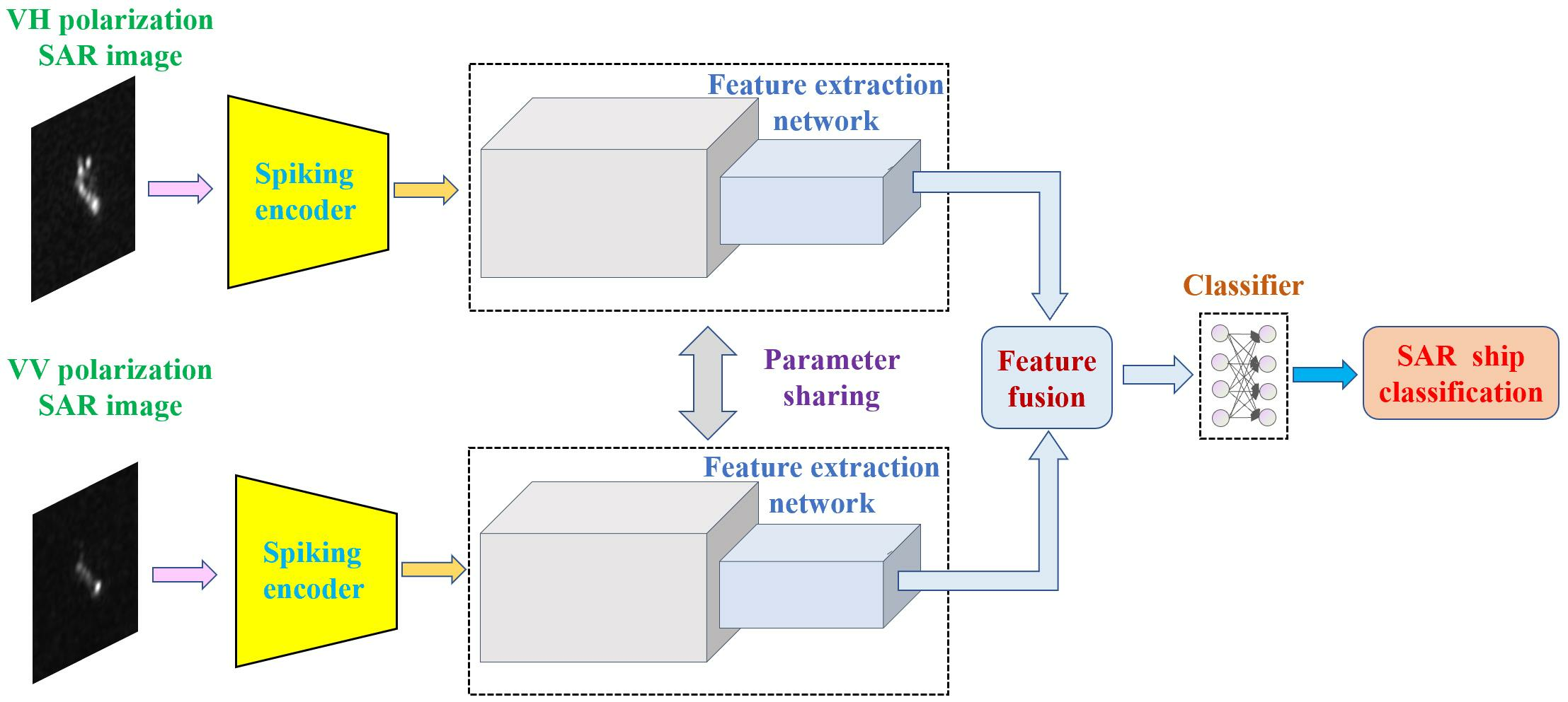
The SNN can run on neural chips and have low energy consumption advantages, making it suitable for deployment on embedded platforms with limited resources. Figure 2 shows the basic architecture of the proposed Siam-SpikingShipCLSNet model. The main body of the proposed model includes a pair of the parameter-shared feature extraction networks, which are used to extract the paired ship features from the dual-polarized SAR images. The extracted ship features are fused in a certain way and then sent to subsequent classification networks for ship classification.
Compared with Siamese networks based on second-generation neural networks such as the convolution neural network (CNN), Siam-SpikingShipCLSNet has significant differences. Firstly, it is based on the third-generation neural network SNNs and uses discrete spiking to transmit the information between neurons. When spiking is transmitted to the neuron, it charges the neuron. If the electric potential exceeds the discharge voltage, the neuron emits a spiking. If there is no spiking transmitted to the current neuron, this neuron is in a resting state and does not work or consume energy. The proposed model is based on frequency encoding, mainly focusing on the frequency of the neurons emitting the spiking without considering the time structure between the spiking sequences. This neural encoding method is a quantitative measure of the output of the neurons. Since it is possible to correspond the spiking firing frequency of neurons within the simulation duration to the continuous values used by the ANN, thus we can draw inspiration from the development achievements of the ANN [32]. Secondly, the model input is a two-dimensional image composed of the continuous values, which needs to be encoded to obtain a two-dimensional spiking matrix that can represent the image information and be understood by the SNN. At the specified simulation time, the backbone network obtains a spiking feature map composed of the discrete 1/0 spiking. Subsequently, the spiking feature map is sent to the classification network, causing the spiking neurons in the output layer to emit the spiking, which represent the network’s judgment of the current input image category. Meanwhile, compared to the ANNs, the SNNs based on frequency encoding have been extended in the temporal dimension. Usually, the simulation step is set to , which means recursively processing the times’ inference of an input image. In this way, multiple output spiking vectors with a length of will be obtained at the output end of the classification network. Finally, the classification result of the model can be determined by calculating the frequency of each spiking neuron in the output layer during the simulation time T. The corresponding category of the neuron with the highest spiking frequency is the model classification result.
2.1. Input Image Spiking Encoding
SNNs use the discrete spike to transmit the information, while the pixel values of the input image are continuous, so it is necessary to encode them into spikes. This paper adopts a stateless Poisson information encoding method to achieve this step. The encoder outputs a two-dimensional 0/1 matrix, and an element value of one in the matrix indicates the presence of a spike at that position. The probability of a spike occurring at a certain position is same as the pixel value of the corresponding position in the normalized input image. The larger the pixel value, the greater the likelihood of emitting a spike. The encoding method of the Poisson encoder is as follows:
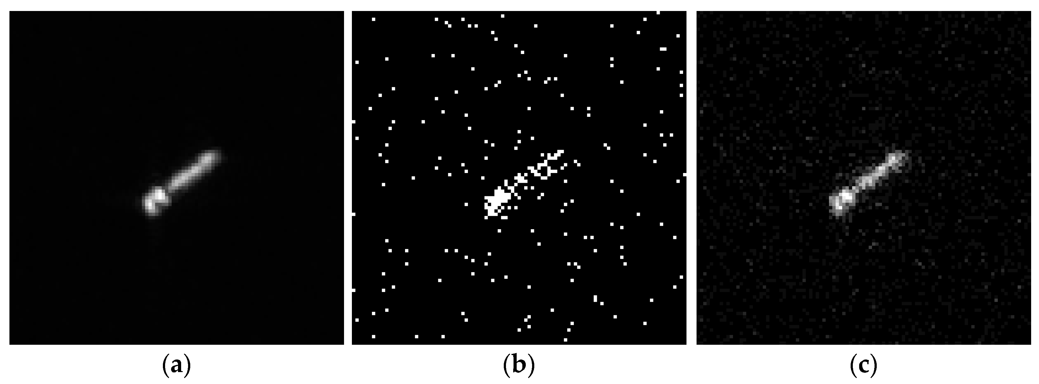
where represents the two-dimensional spiking matrix output by the encoder, represents the input image, and represents a uniform distribution. is a random variable following a 0–1 distribution, and its values are used as thresholds to binarize continuous pixel values. During the simulation step , a two-dimensional spiking sequence with a length of is obtained. There may be a loss of the image information in the process of converting the continuous pixel value to the discrete two-dimensional map, but this information loss can be greatly reduced after pulses. Figure 3 gives an example of visualizing the spiking results using the Poisson encoding. It is seen that although there are differences between the two-dimensional spiking matrix and the original image, it fully preserves the main information of the original image. At the same time, there is also a discrete spiking point caused by the presence of coherent spots in the background. In the actual process of the automatic target recognition, the front-end target detector accurately locates the target and then intercepts it, which can avoid these discrete spiking points.
2.2. Spiking Neuron Model
An SNN is composed of the spiking neurons, and the selection of the spiking neurons affects the overall performance of the SNN model. The typical spiking neuron model includes the Hodgkin Huxley (H-H) model [33], IF model [34], leaky integrate and fire (LIF) model [35], and so on. The H-H spiking neuron model has a strong biological interpretability, but the model is too complex to construct. The IF model is too simplistic and directly uses the capacitors to describe the working process of the neurons, without describing the particle diffusion phenomenon that exists in the biological neurons. The LIF model is an improvement on the IF spiking neuron model. The LIF model considers another physiological factor: the cell membrane is not a perfect capacitor and the charge slowly leaks through the cell membrane over time, allowing the membrane voltage to return to its resting potential [35]. In this paper, the LIF spiking neuron model is adopted to build a Siamese SNN for the SAR ship classification. The main actions of the spiking neurons include the charging, discharging, and resting, so the corresponding model needs to provide the corresponding descriptions. The differential equations of the LIF model is given by:
where is the time constant, is the capacitor, and is the input impedance. is the capacitor voltage, is the resting potential, and is the current flowing through the capacitor. The change in the voltage during the charging process can be described by the following:
If the membrane voltage exceeds the threshold, the neuron emits spikes, and then the membrane voltage drops to the reset potential .
In practice, the discrete difference equation is generally used to describe the charging, discharging, and resetting actions of the LIF spiking neurons, which is as follows:
Equation (4) represents the change in the neuronal potential during charging. is the input spiking of the neuron, is the state update function of the neuron charging moment, is the membrane voltage of the neuron, and is the spiking sequence emitted by the neuron with a value of 0 or 1. is the spike firing state of the neuron, is the Step function, is the threshold voltage of the spiking emission. Equation (6) represents the hard-reset voltage after transmitting the spike.
2.3. Backbone Network Structure
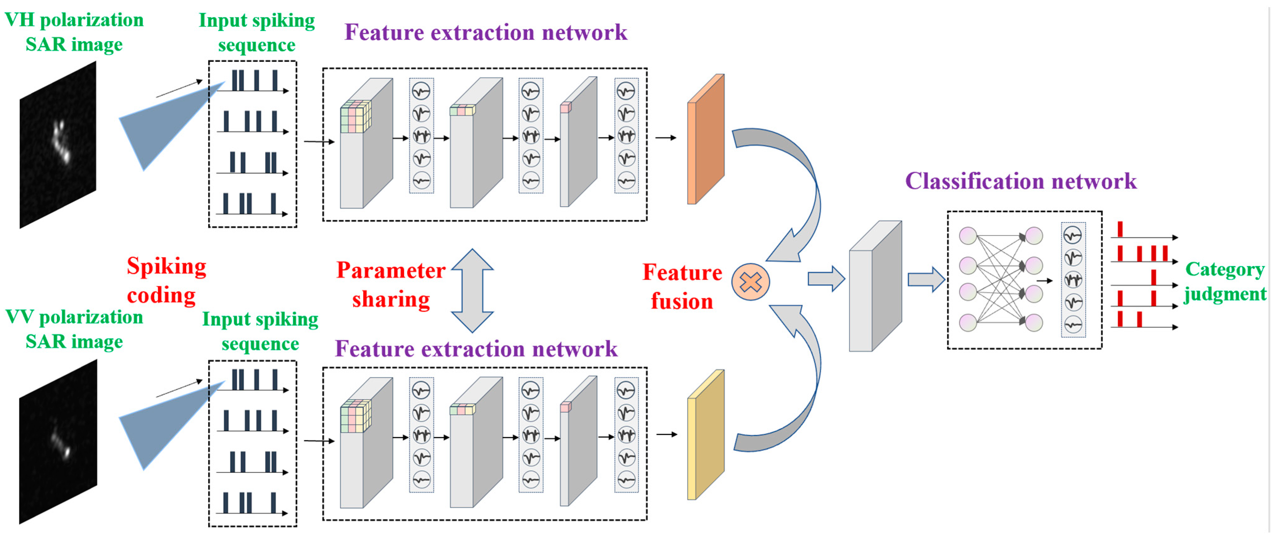
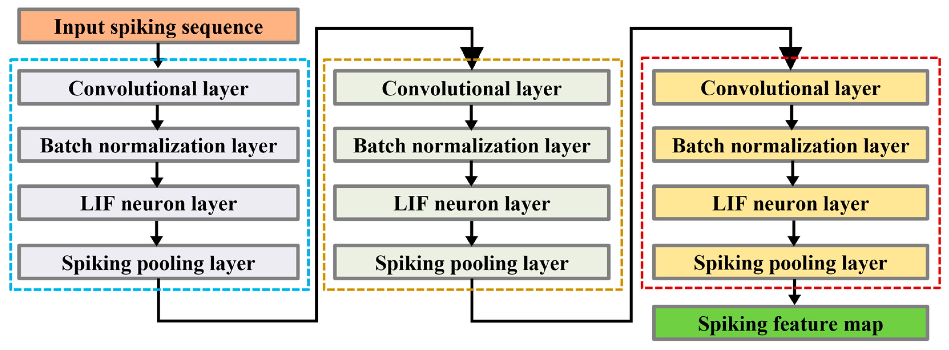
The overall model of the proposed Siam-SpikingShipCLSNet is shown in Figure 2. The backbone network is parameter shared and used to extract the feature from the input SAR ship images, whose specific structure is shown in Figure 4. The network structure is constructed by stacking the spiking convolutional network blocks, and the backbone network consists of three spiking convolution blocks. A single spiking convolution block consists of a convolutional layer, a batch normalization layer, an LIF neuron layer, and a spiking pooling layer. The maximum spiking pooling is selected based on the research [29], which suggests that the ability of the maximum pooling to process the information is consistent with that of the SNNs, which is beneficial for fitting the temporal data. The backbone network adopts a shallow design to ensures the lightweight network. In addition, the SAR ship image does not have rich feature information, the performance improvement brought by using the deep network is not significant, but the consumption of the computing resources is greater. In addition, this paper adopts an alternative gradient training method, where the gradient is approximate. If a deep network architecture is used, the approximation error of the gradient will gradually accumulate and amplify with the increase in the network depth, which will affect the convergence of the model. The data pass through three spiking convolution blocks to obtain a spiking feature map with a down-sampling rate of eight, which characterizes the feature information of the input image. After the spiking feature fusion processing, it is sent to the target classification network for ship classification.
2.4. Spiking Feature Fusion
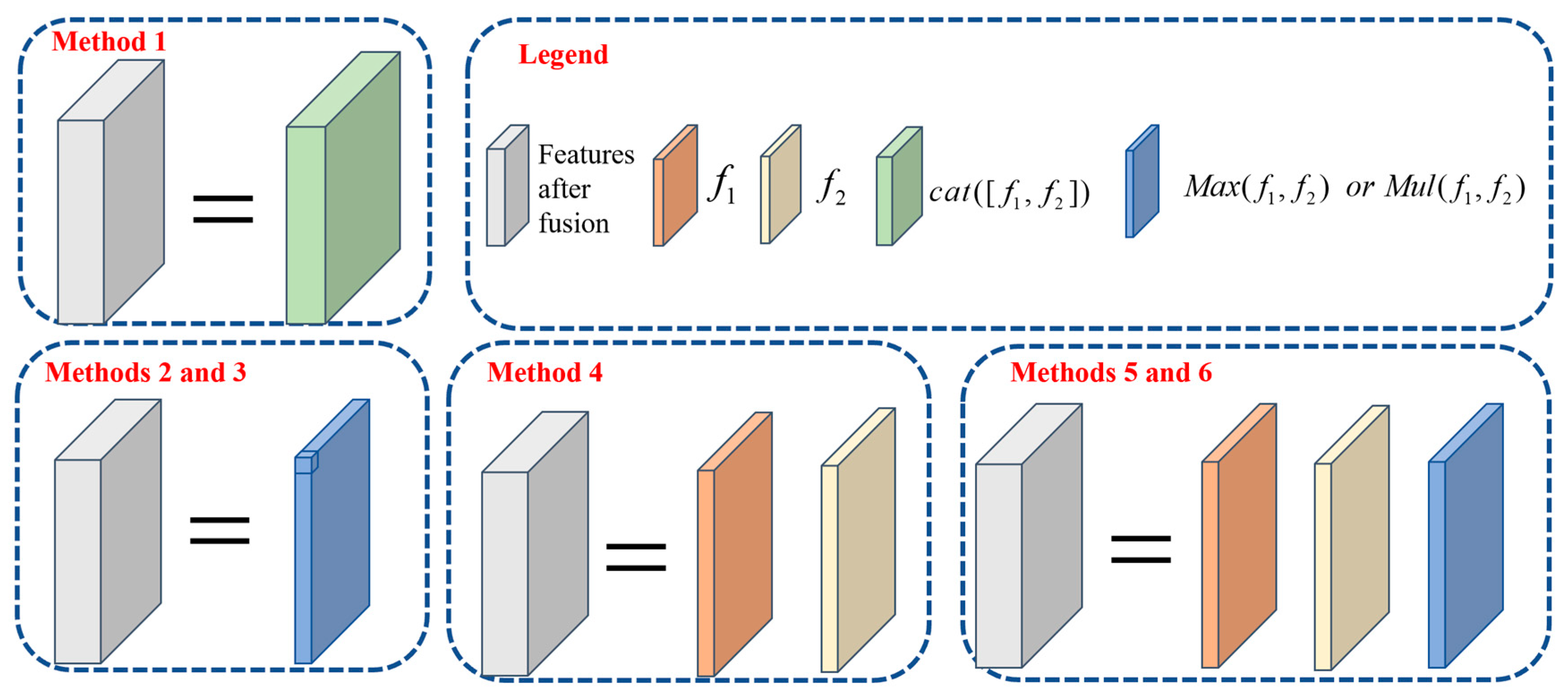
The key of the proposed Siamese SNN is the fusion of the spiking features extracted from the backbone network. This paper proposes six fusion methods based on the data fusion idea in the ANN, as shown in Figure 5.
It can be assumed that the spiking features of the dual-polarized ship images extracted by the backbone network are and , and the mapping relationship of the fully connected layer is represented by . Therefore, under the fusion modes, the network output can be represented by the various formulas in Table 1.
represents concatenating dual-polarized spiking feature maps in the channel dimension, then feeding them into the subsequent classifiers. indicates taking the maximum element-wise on the corresponding channel of the dual-polarization spiking feature map. In other words, as long as any prior neuron in either branch of the Siamese network emits a pulse, that pulse should be retained. This processing aims to fully utilize the useful features and enhance the firing rate of the spiking neurons. represents the multiplication operation on each channel of the dual-polarized spiking feature map, which means that only the prior neurons in both main networks emit spiking and can be transmitted to the post neurons. This processing aims to enhance common features in the dual-polarized images. Compared to the first three methods, the latter three fusion methods not only fuse the spiking features of the dual-polarized methods, but also send the original spiking features into the classification network for fusion at the output layer.
2.5. Model Learning Methods
The SNNs cannot directly use the gradient descent backpropagation training methods due to their nondifferentiable neural function. Thus, it is necessary to design the algorithms for the error backpropagation of the spiking sequences. SNN learning and optimization methods mainly include the learning rule based on the error backpropagation, learning rule based on the spike-timing dependent plasticity (STDP), and the ANN-to-SNN learning rule. Because the proposed Siam-SpikingShipCLSNet model belongs to a convolutional SNN based on the frequency information encoding, an end-to-end error backpropagation optimization algorithm based on the surrogate gradient is adopted.
2.5.1. Surrogate Gradient Training
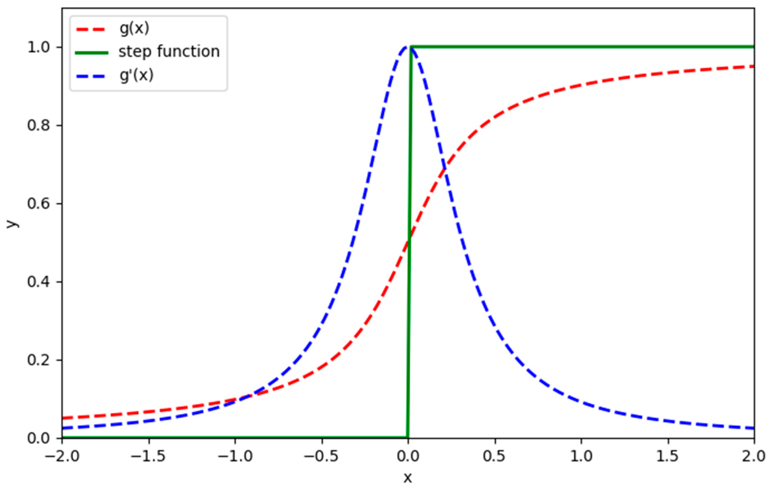
The spiking signal emitted by the spiking neurons during the forward propagation is used to transmit the information. The discharge function of the neurons is a Step function, and the corresponding derivative function is an impulse function, so it cannot be used for the directional propagation optimization algorithm based on the gradient descent [36]. For the proposed model based on the frequency information encoding, the neuron spiking frequency in the output layer characterizes the model classification results. Thus, this paper first calculates the error between it and its label, and then updates the network parameters through the error backpropagation based on the surrogate gradient. The error backpropagation algorithm based on the surrogate gradient refers to the use of the original discharge function of the spiking pulse neurons in (5) in the forward inference of the model, and the use of the approximate differentiable function to update the network parameter in the backpropagation calculation of the gradients. In this paper, the model uses the arctangent function as the surrogate function, which is as follows:
where α takes a value of 2 in this experiment, and the image of the surrogate function is shown in Figure 6. It is indicated that it can have a shape similar to that of the Step function, and its derivative function is also a sharp curve similar to the impact function.
2.5.2. Loss Function
SNNs based on the frequency information encoding have a higher spiking frequencies output through more excited neurons. Therefore, in the output spiking neuron layer, the category represented by the neuron with the highest spiking frequency can be used as the model classification result. This logic is consistent with the labels that use the one-hot encoding, where the position element corresponding to the specified category has the highest value, with a value of 1 and the rest being 0. Therefore, the neuron spiking emission frequency in the output layer and the distance between the labels can be used to measure the model prediction error. In this paper, the loss function uses the mean square error function, which is as follows:
where is a vector that represents the number of spikes emitted by each neuron in the output layer. represents the network output vector, which is equal to the vector divided by the simulation step , where represents the number of the categories and represents the label.
3. Experimental Results and Analysis
3.1. Experimental Setup
For ship classification, the high or very high-resolution SAR images will provide excellent results [37,38]. Nowadays, the low-medium resolution dataset is still used for the ship classification in SAR images. In this paper, the OpenSARShip2.0 dataset released by the Shanghai Jiao Tong University [8] is adopted as the experimental data, which include 34,528 SAR ship image slices, mainly obtained from the Sentinel-1 satellite SAR system. It includes two interference wideband modes, i.e., the single look complex (SLC) and ground range detected (GRD). Each ship SAR image slice is verified by a maritime traffic website or automatic identification system (AIS) to ensure the accuracy of the label. The resolution of the GRD mode is 20 × 22 m, while the resolution of the SLC mode is from 2.7 × 22 m to 3.5 × 22 m. The imaging area of the SAR image slice includes many port regions such as Shanghai and Shenzhen, and there is no interference such as the land background. The same ship contains the slice pairs of the VV and VH polarization modes. There are more than ten types of the ship categories in the entire dataset, but the distribution of the category numbers is extremely imbalance. Usually, several of them are selected for the experiments and analysis. In this paper, a relatively large number of Cargo (with chip number 21,241), Tanker (with chip number 6343), Fishing (with chip number 454), and Other-type (with chip number 5224) ships were selected for the ship classification in these experiments.
The number of the SAR images in the training set and test set is divided in a ratio of 3:1, and the input SAR image size is adjusted to 64 × 64. The Adam optimizer is used for the model training. For the neural network trained in this experiment, the batchsize is set to 32, and the learning rate is set to 0.0001. In the above dataset, the experiment uses a server equipped with the graphics card of the NVIDIA GeForce 3090 and central processing unit (CPU) of the Intel (R) Xeon (R) E5-2678 v3 @ 2.50 GHz model. The operating system is ubuntu 22.04 LTS, the software development uses the Pytorch 1.13 framework and accelerates the model using the CUDA11.7.
3.2. Evaluating Indicator
In this paper, the common evaluation indicators in the image classification field are used to evaluate the classification performance of models involved in this experiment, mainly including the precision, recall rate, and score [17,18,37]. The precision, recall rate, and score of the ship classification for the single category SAR images can be given as follows:
where represents the number of the correctly classified targets in this category, represents the number of the falsely classified targets in this category, and represents the number of the falsely negative targets in this category that are only classified as the other categories. Due to the imbalance in the distribution of the number of ship targets on the various types, for a fair evaluation, the proportion of the number of the ship images is used as a weighting factor to calculate the weighting value as the overall evaluation indicators. The specific formulas are as follows:
where represents the number of all SAR images, represents the number of the SAR images of the i-th category, and represents the number of the categories. The weighted recall rate is equal to the accuracy, which is the proportion of all correctly predicted samples to the total number of the samples.
In addition, to evaluate the complexity of the models, the model parameter quantity and number of the operations are used for analysis. For the ANN-based models, the floating-point operations numbers (FLOPs) are used for evaluating the computation complexity, while for the SNN-based models, the synaptic operation numbers (SOPs) are used for evaluating the computation complexity [39], which is given by:
where is the number of the spiking emitted by the current spiking neuron layer, and is the number of the connection between the current spiking neuron layer and the subsequent layer. For an SNN, the computation is only generated when neurons emit spikes. Therefore, based on the above Equation (17), the total computation count within the simulation step size T can be calculated.
3.3. Experiment and Analysis
3.3.1. Ship Classification Performance
To verify the effectiveness of the proposed Siam-SpikingShipCLSNet model, the experiment compared the models with multiple paradigms. The mainstream classification network based on the convolutional neural network (CNN) selects the ResNet (including 18, 34, and 50 depths) [40], the densely connected convolutional network (DenseNet) (including 121 and 161 sizes) [41], VGG16 [42], MobileNet-v2 [43], and AlexNet [44]. The classification network based on the visual Transformer selects the ViT [45] and ResNet50ViT. ResNet50ViT is the fusion of the CNN and ViT, which first uses the backbone network of the ResNet50 to extract the image features, then sends the features to the ViT for the further learning and finally gives the classification results. The network selection based on the SNN architecture is Spiking-ResNet18 [46], which is the result of the spiking transformation of the CNN-ResNet18. The comparative experimental results are summarized in Table 2.
Based on the experimental data, it is not difficult to find that the proposed Siam- SpikingShipCLSNet performs the better than the most mainstream CNN classification models, with the model precision and recall scores of 0.6395 and 0.6735, respectively, which is higher than all comparisons shown in Table 2. The F1 score is 0.6365, only lower than the 0.6389 and 0.6436 obtained by the DenseNet121 and DenseNet161. Therefore, it can be considered that the proposed Siam-SpikingShipCLSNet model can achieve the performance level of the mainstream classification network models. Secondly, the Spiking-ResNet18 model based on the SNN architecture has certain disadvantages compared with the model based on the Siamese CNN architecture. One of the main reasons is that as a third-generation ANN, it still has many immature aspects, and its network structure design, training methods, neuron design, and other tasks are more difficult compared to the CNN. Fortunately, its prospect of ultra-low energy consumption has attracted the attention of a large number of applications.
3.3.2. Model Parameter Quantity
The model parameter quantity is also one of the important evaluation indicators for evaluating the resource utilization demand of the model. Nowadays, many open-source frameworks provide interfaces for computing this metric. When the performance difference of the model is small, the strong advantages of the model with the small parameter quantity will be demonstrated during the deployment. Although the performance of the CNN is gradually improving in various tasks, the network size is also starting to rise, so it is necessary to evaluate its parameter quantity.
Table 3 shows the parameter size of the experimental models, and the unit of the data is M. From Table 3, it is found that the proposed Siam-SpikingShipCLSNet model has the parameter quantity of only 2.19 M, which is lower compared with the other mainstream image classification networks. In addition, its parameter quantity mainly comes from the fully connected layer. If the method 2 of the data fusion is used, the model parameter quantity will only be 1.15 M.
3.3.3. Model Energy Consumption
This section discusses the computational complexity of various experimental models, which is evaluated by the number of operations required for a single inference. For models based on the second-generation ANN, the floating-point operations are used for evaluation, whereas for models based on the SNN, the computational complexity is calculated by the formula provided in reference [39], i.e., Equation (17). Moreover, the model energy consumption depends on both the number of operations of the model itself and the hardware devices deployed by the model. This paper assumes that the experimental model based on the second-generation ANN runs on an advanced and efficient computing device (Intel Stratix 10 TX FPGA) with an energy consumption of 12.5 pJ/FLOP, while the experimental model based on the SNN runs on the neural morphology chip ROLLS [31] with an energy consumption of 77 fJ/SOP. The computational complexity and energy consumption of each experimental model are shown in Table 4. From Table 4, it is not difficult to find that the SNN-based model Spiking-ResNet18 and proposed Siam-SpikingShipCLSNet model consume three orders of the magnitude less energy for the single inference than other models based on the CNN and Transformer architectures. In addition, the proposed Siam-SpikingShipCLSNet model achieves the lowest energy consumption in experimental models, which is less than half of the energy consumption of the Spiking-ResNet18 model. Due to the lower energy consumption advantage of the SNN, it has the great application prospects in the platforms with limited energy.
3.3.4. Fusion Method Analysis
This section analyzes the performance differences and reasons for the proposed Siam-SpingShipCLSNet based on the different spiking feature fusion methods, and the experimental results are shown in Table 5. SOP/T represents the number of the synaptic operations generated in a single forward inference, which can be used to evaluate the spiking firing rate of the SNN neurons. According to the experimental results, it has been found that the experimental group that does not use the Siamese network architecture to fuse the dual-polarized SAR images had the lower precision, recall, and F1 scores than the other six groups that used the Siamese SNN architecture. This demonstrates the superiority of the Siamese network fusion architecture for ship classification using dual-polarized SAR images.
In six experiments based on the Siamese SNN architecture, it is not difficult to find that spiking feature fusion method 1 achieved the best performance, which are selected as the final data fusion method in this paper. This is mainly because it entrusts the stitching of the spiking features from dual-polarized SAR ship images to a fully connected layer that can learn the subsequent parameters for the fusion, which increases the width and fusion ability of the fully connected layer compared to other methods. Similarly, this increases the number of the parameters in the network, but it achieves optimal performance at a simulation step of eight, resulting in a lower operation number. Fusion method 3 has the worst performance due to the operation of the element-by-element multiplication, which only preserves the key features that are common to both dual-polarized SAR ship images, resulting in the information loss. In addition, its operation number is lower than that of fusion method 2 (the simulation step is 20), because some spikes are suppressed by the element-by-element multiplication processing, resulting in a decrease in the spiking emission rate of the spiking neurons. On the other hand, fusion method 6 adds two original features on fusion method 3, compensating for the information loss caused by the element-by-element multiplication, and then the common spiking features are retained. In addition, the element-by-element multiplication can serve as the attention mechanism to enhance the attention to the common key features. Therefore, fusion method 6 performs better than fusion method 3 and fusion method 4 (without the two spiking feature operation processing). Fusion method 2 uses the maximum value of each element to fuse the spiking features of two sources, retaining most of the features of the dual-polarized spiking, thus, its performance is superior to fusion method 3 and the spiking emission rate is higher than that of fusion method 3. Although the element-by-element maximum process is also used in fusion method 5, due to its inclusion of two original spiking features, this process did not effectively increase the information but added more noise. So, the performance of fusion method 5 was not significantly improved compared to fusion method 2.
3.3.5. Simulation Step Analysis
This section discusses the relationship between the simulation step and the performance of the proposed Siam-SpikingShipCLSNet model. In general, the SNN based on the frequency information encoding need to set a certain simulation step to achieve a certain performance. A higher simulation step will cause a decrease in the model running speed and an increase in the model computational complexity, while a lower simulation step will cause the significant performance degradation. Thus, the setting of the simulation step needs to be determined through multiple experiments. Table 6, Table 7, Table 8, Table 9, Table 10 and Table 11 show the impact of the different simulation steps on the performance of the model under six data fusion methods. For fusion method 1 in Table 6, although the F1 score is better when the simulation step is set to 12 or 20 than when the simulation step is 8, there is no significant advantage in the precision and recall, which are even lower, and the increase in the operands is greater. Thus, a simulation step of 8 is selected for fusion method 1. For fusion method 2 in Table 7, as the simulation step continues to increase, the precision, recall, F1 score, and computational complexity all increase. Thus, the simulation step corresponding to the optimal performance is selected. For fusion method 3 in Table 8, due to the information loss caused by the element-by-element multiplication operation, increasing the simulation step can reduce the degree of the information loss, thus achieving the optimal performance at a simulation step of 20. So, for fusion method 3, the simulation step is also set to 20. For fusion method 4 in Table 9, although the F1 score reaches its maximum value when the simulation step is 12, the accuracy and recall are low, so the simulation step is set to 16. For fusion method 5 in Table 10, the optimal performance is achieved at a simulation step of 16. Increasing the simulation step to 20 resulted in a decrease in the performance, which may be because further increasing the simulation step when the simulation step is enough does not provide more information but introduces more noise. For fusion method 6 in Table 11, when the simulation step is set to 16, the F1 score is the highest, and compared to when the step is set to 12, the increment is significant. The precision and recall are similar to when the step is set to 12, so 16 is chosen as final simulation step.
Based on the above experimental data, the final data fusion method in this paper adopts fusion method 1 and the simulation step is set to eight, because under these conditions, its classification ability is optimal with the lowest number of the operations and the shortest simulation step. The length of simulation steps can ensure the model speed, and a low number of operations can ensure the low energy consumption of the model.
4. Conclusions
Firstly, due to the lack of the obvious features and small inter-class differences in the SAR ship images, SAR ship recognition has become a challenging task. Secondly, the existing SAR ship image dataset has a limited data and imbalanced class distribution, which is not conducive to learning of deep learning models. At last, SAR imaging has different polarization modes, and the images under different polarization modes contain different information about the same target, which should be comprehensively utilized to improve the recognition ability of the network.
Traditional deep learning methods have the problem of an excessive model parameter number and high energy consumption for the SAR ship classification, thus, this paper has proposed an energy-efficient and high-performance ship classification strategy based on the Siamese SNN. It combines the advantages of SNN in energy consumption and the advantage of the idea in performances that use the Siamese neuron network to fuse the features from dual-polarized SAR images. Additionally, we migrated the feature fusion strategy from the CNN-based Siamese neural networks to the SNN domain and then analyzed the effects of various spiking feature fusion methods on the Siamese SNN. Finally, an end-to-end error backpropagation optimization method based on the surrogate gradient has been adopted to train this model. The ship classification experiment has been conducted on the OpenSARShip2.0 dataset, which shows that the proposed strategy achieves the performance of the existing mainstream classification models with a smaller number of parameters and much lower energy consumption than the mainstream classification models. In the further work, more effective information (such as prior information such as SAR imaging characteristics) and more effective fusion methods should be conducted, as well as a comparison with other similar approaches [47,48].
Author Contributions
Conceptualization, X.J. and H.X.; methodology, X.J. and H.X.; software, X.J. and H.X.; validation, X.J. and H.X.; formal analysis, X.J. and H.X.; investigation, X.J. and H.X.; resources, H.X. and Z.L.; data curation, H.X. and J.H.; writing—original draft preparation, X.J. and H.X.; writing—review and editing, X.J., H.X., Z.L. and J.H.; visualization, X.J. and H.X.; supervision, H.X. and J.H.; project administration, H.X. and J.H.; funding acquisition, H.X., J.H. and Z.L. All authors have read and agreed to the published version of the manuscript.
Funding
This research was co-supported by the Guangdong Basic and Applied Basic Research Foundation (Grant Nos. 2021A1515010768 and 2023A1515011588), the Shenzhen Science and Technology Program (Grant Nos. 202206193000001, 20220815171723002), the Beijing Nova Program (Grant No. Z201100006820103), and the National Natural Science Foundation of China (Grant Nos. 62001523, 62203465, 62201614, and 6210593). Hongtu Xie is the corresponding author.
Data Availability Statement
Not applicable.
Acknowledgments
The authors would like to thank the editors and reviewers for their very competent comments and helpful suggestions to improve this paper. We would also like to thank the Shanghai Jiao Tong University for providing the OpenSARShip2.0 datasets.
Conflicts of Interest
The authors declare no conflict of interest.
References
- Huang, J.; An, D.; Chen, L.; Feng, D.; Zhou, Z. An NSST-Based Fusion Method for Airborne Dual-Frequency, High-Spatial-Resolution SAR Images. IEEE J. Sel. Top. Appl. Earth Obs. Remote Sens. 2023, 16, 4362–4370. [Google Scholar] [CrossRef]
- Ge, B.; An, D.; Liu, J.; Feng, D.; Chen, L.; Zhou, Z. Modified Adaptive 2-D Calibration Algorithm for Airborne Multichannel SAR-GMTI. IEEE Geosci. Remote Sens. Lett. 2023, 20, 4004805. [Google Scholar] [CrossRef]
- Luo, Y.; An, D.; Wang, W.; Chen, L.; Huang, X. Local Road Area Extraction in CSAR Imagery Exploiting Improved Curvilinear Structure Detector. IEEE Trans. Geosci. Remote Sens. 2022, 60, 3172227. [Google Scholar] [CrossRef]
- Chen, J.; Xie, H.; Zhang, L.; Hu, J.; Jiang, H.; Wang, G. SAR and Optical Image Registration Based on Deep Learning with Co-Attention Matching Module. Remote Sens. 2023, 15, 3879. [Google Scholar] [CrossRef]
- Zhu, J.; Song, Y.; Jiang, N.; Xie, Z.; Fan, C.; Huang, X. Enhanced Doppler Resolution and Sidelobe Suppression Performance for Golay Complementary Waveforms. Remote Sens. 2023, 15, 2452. [Google Scholar] [CrossRef]
- Hu, X.; Xie, H.; Zhang, L.; Hu, J.; He, J.; Yi, S.; Jiang, H.; Xie, K. Fast Factorized Backprojection Algorithm in Orthogonal Elliptical Coordinate System for Ocean Scenes Imaging Using Geosynchronous Spaceborne-Airborne VHF UWB Bistatic SAR. Remote Sens. 2023, 15, 2215. [Google Scholar] [CrossRef]
- Jiang, X.; Xie, H.; Chen, J.; Zhang, J.; Wang, G.; Xie, K. Arbitrary-Oriented Ship Detection Method Based on Long-Edge Decomposition Rotated Bounding Box Encoding in SAR Images. Remote Sens. 2023, 15, 673. [Google Scholar] [CrossRef]
- Li, B.; Liu, B.; Huang, L.; Guo, W.; Zhang, Z.; Yu, W. OpenSARShip 2.0: A Large-Volume Dataset for Deeper Interpretation of Ship Targets in Sentinel-1 Imagery. In Proceedings of the SAR in Big Data Era: Models, Methods and Applications (BIGSARDATA), Beijing, China, 13–14 November 2017; pp. 1–5. [Google Scholar]
- Xie, H.; Jiang, X.; Zhang, J.; Chen, J.; Wang, G.; Xie, K. Lightweight and Anchor-Free Frame Detection Strategy Based on Improved CenterNet for Multiscale Ships in SAR Images. Front. Comput. Sci. 2022, 4, 1012755. [Google Scholar] [CrossRef]
- Xie, H.; Jiang, X.; Hu, X.; Wu, Z.; Wang, G.; Xie, K. High-Efficiency and Low-Energy Ship Recognition Strategy Based on Spiking Neural Network in SAR Images. Front. Neurorobot. 2022, 16, 970832. [Google Scholar] [CrossRef]
- Xie, H.; He, J.; Lu, Z.; Hu, J. Two-Level Feature-Fusion Ship Recognition Strategy Combining HOG Features with Dual-Polarized Data in SAR Images. Remote Sens. 2023, 15, 3928. [Google Scholar] [CrossRef]
- Xi, Y.; Xiong, G.; Yu, W. Feature-Loss Double Fusion Siamese Network for Dual-Polarized SAR Ship Classification. In Proceedings of the IEEE International Conference on Signal, Information and Data Processing (ICSIDP), Chongqing, China, 11–13 December 2019; pp. 1–5. [Google Scholar]
- He, J.; Chang, W.; Wang, F.; Wang, Q.; Li, Y.; Gan, Y. Polarization Matters: On Bilinear Convolutional Neural Networks for Ship Classification from Synthetic Aperture Radar Images. In Proceedings of the International Conference on Natural Language Processing (ICNLP), Xi’an, China, 25–27 March 2022; pp. 315–319. [Google Scholar]
- He, J.; Chang, W.; Wang, F.; Liu, Y.; Wang, Y.; Liu, H.; Li, Y.; Liu, L. Group Bilinear CNNs for Dual-Polarized SAR Ship Classification. IEEE Geosci. Remote Sens. Lett. 2022, 19, 4508405. [Google Scholar] [CrossRef]
- Shao, Z.; Zhang, T.; Ke, X. A Dual-Polarization Information-Guided Network for SAR Ship Classification. Remote Sens. 2023, 15, 2138. [Google Scholar] [CrossRef]
- Zhang, T.; Zhang, X. Squeeze-and-Excitation Laplacian Pyramid Network with Dual-polarization Feature Fusion for Ship Classification in SAR Images. IEEE Geosci. Remote Sens. Lett. 2021, 19, 4019905. [Google Scholar] [CrossRef]
- Zhang, T.; Zhang, X.; Ke, X.; Liu, C.; Xu, X.; Zhan, X.; Wang, C.; Ahmad, I.; Zhou, Y.; Pan, D.; et al. HOG-ShipCLSNet: A Novel Deep Learning Network with HOG Feature Fusion for SAR Ship Classification. IEEE Trans. Geosci. Remote Sens. 2022, 60, 5210322. [Google Scholar] [CrossRef]
- Lin, H.; Song, S.; Yang, J. Ship Classification Based on MSHOG Feature and Task-Driven Dictionary Learning with Structured Incoherent Constraints in SAR Images. Remote Sens. 2018, 10, 190. [Google Scholar] [CrossRef]
- Devlin, J.; Chang, M.; Lee, K.; Toutanova, K. BERT: Pre-training of Deep Bidirectional Transformers for Language Understanding. In Proceedings of the Conference of the North American Chapter of the Association for Computational Linguistics: Human Language Technologies (NAACL-HLT), Minneapolis, MN, USA, 2–7 June 2019; pp. 4171–4186. [Google Scholar]
- Fedus, W.; Zoph, B.; Shazeer, N. Switch Transformers: Scaling to Trillion Parameter Models with Simple and Efficient Sparsity. J. Mach. Learn. Res. 2022, 23, 5232–5270. [Google Scholar]
- Brown, T.; Mann, B.; Ryder, N.; Subbiah, M.; Kaplan, J.; Dhariwal, P.; Neelakantan, A.; Shyam, P.; Sastry, G.; Askell, A.; et al. Language Models Are Few-Shot Learners. Adv. Neural Inf. Process. Syst. 2020, 33, 1877–1901. [Google Scholar]
- Maass, W. Networks of Spiking Neurons: The Third Generation of Neural Network Models. Neural Netw. 1997, 10, 1659–1671. [Google Scholar] [CrossRef]
- Roy, K.; Jaiswal, A.; Panda, P. Towards Spike-Based Machine Intelligence with Neuromorphic Computing. Nature 2019, 575, 607–617. [Google Scholar] [CrossRef]
- Buhmann, J.; Lange, T.; Ramacher, U. Image Segmentation by Networks of Spiking Neurons. Neural Comput. 2005, 17, 1010–1031. [Google Scholar] [CrossRef]
- Cui, W.; Lin, X.; Xu, M. Coding Method of Image Segmentation in Spiking Neural Network. Comput. Eng. 2012, 38, 196–199. [Google Scholar]
- Kim, S.; Park, S.; Na, B.; Yoon, S. Spiking-Yolo: Spiking Neural Network for Energy-Efficient Object Detection. In Proceedings of the AAAI Conference on Artificial Intelligence (CAI), New York, NY, USA, 7–12 February 2020; pp. 11270–11277. [Google Scholar]
- Luo, Y.; Shen, H.; Cao, X.; Wang, T.; Feng, Q.; Tan, Z. Conversion of Siamese Networks to Spiking Neural Networks for Energy-Efficient Object Tracking. Neural Comput. Appl. 2022, 34, 9967–9982. [Google Scholar] [CrossRef]
- Merolla, P.; Arthur, J.; Alvarez-Icaza, R.; Cassidy, A.S.; Sawada, J.; Akopyan, F.; Jackson, B.L.; Imam, N.; Guo, C.; Nakamura, Y.; et al. A Million Spiking-Neuron Integrated Circuit with A Scalable Communication Network and Interface. Science 2014, 345, 668–673. [Google Scholar] [CrossRef]
- Fang, W.; Yu, Z.; Masquelier, T.; Chen, Y.; Huang, T.; Tian, Y. Spike-Based Residual Blocks. arXiv 2021, arXiv:2102.04159. [Google Scholar]
- Bu, T.; Fang, W.; Ding, J.; Dai, P.; Yu, Z.; Huang, T. Optimal ANN-SNN Conversion for High-Accuracy and Ultra-Low-Latency Spiking Neural Networks. arXiv 2023, arXiv:2303.04347. [Google Scholar]
- Indiveri, G.; Corradi, F.; Qiao, N. Neuromorphic Architectures for Spiking Deep Neural Networks. In Proceedings of the IEEE International Electron Devices Meeting (IEDM), Washington, DC, USA, 7–9 December 2015; pp. 4.2.1–4.2.4. [Google Scholar]
- Hu, Y.; Li, G.; Wu, Y.; Deng, L. Spiking Neural Networks: A Survey on Recent Advances and New Directions. Control. Decis. 2021, 36, 1–26. [Google Scholar]
- Hodgkin, A.; Huxley, A. A Quantitative Description of Membrane Current and Its Application to Conduction and Excitation in Nerve. Bull. Math. Biol. 1989, 52, 25–71. [Google Scholar] [CrossRef]
- Dayan, P.; Abbott, L. Theoretical Neuroscience: Computational and Mathematical Modeling of Neural Systems. J. Cogn. Neurosci. 2003, 15, 154–155. [Google Scholar]
- Gerstner, W.; Kistler, W.; Naud, R.; Paninski, L. Neuronal Dynamics: From Single Neurons to Networks and Models of Cognition; Cambridge University Press: New York, NY, USA, 2014. [Google Scholar]
- Eshraghian, J.; Ward, M.; Neftci, E.; Wang, X.; Lenz, G.; Dwivedi, G.; Bennamoun, M.; Jeong, D.S.; Lu, W.D. Training Spiking Neural Networks Using Lessons from Deep Learning. arXiv 2021, arXiv:2109.12894. [Google Scholar] [CrossRef]
- Wang, Y.; Wang, C.; Zhang, H. Ship Classification in High-resolution SAR Images Using Deep Learning of Small Datasets. Sensors 2018, 18, 2929. [Google Scholar] [CrossRef]
- Lu, C.; Li, W. Ship Classification in High-Resolution SAR Images via Transfer Learning with Small Training Dataset. Sensors 2018, 19, 63. [Google Scholar] [CrossRef] [PubMed]
- Rueckauer, B.; Lungu, I.; Hu, Y.; Pfeiffer, M.; Liu, S.-C. Conversion of Continuous-Valued Deep Networks to Efficient Event-driven Networks for Image Classification. Front. Neurosci. 2017, 11, 682. [Google Scholar] [CrossRef]
- He, K.; Zhang, X.; Ren, S.; Sun, J. Deep Residual Learning for Image Recognition. In Proceedings of the IEEE Conference on Computer Vision and Pattern Recognition (CVPR), Las Vegas, NV, USA, 27–30 June 2016; pp. 770–778. [Google Scholar]
- Huang, G.; Liu, Z.; Van Der Maaten, L.; Weinberger, K. Densely Connected Convolutional Networks. In Proceedings of the IEEE Conference on Computer Vision and Pattern Recognition (CVPR), Honolulu, HI, USA, 21–26 July 2017; pp. 2261–2269. [Google Scholar]
- Simonyan, K.; Zisserman, A. Very Deep Convolutional Networks for Large-Scale Image Recognition. arXiv 2014, arXiv:1409.1556. [Google Scholar]
- Howard, A.; Zhu, M.; Chen, B.; Kalenichenko, D.; Wang, W.; Weyand, T.; Andreetto, M.; Adam, H. MobileNets: Efficient Convolutional Neural Networks for Mobile Vision Applications. arXiv 2017, arXiv:1704.04861. [Google Scholar]
- Krizhevsky, A.; Sutskever, I.; Hinton, G. ImageNet Classification with Deep Convolutional Neural Networks. Commun. ACM 2017, 60, 84–90. [Google Scholar] [CrossRef]
- Dosovitskiy, A.; Beyer, L.; Kolesnikov, A.; Weissenborn, D.; Zhai, X.; Unterthiner, T.; Dehghani, M.; Minderer, M.; Heigold, G.; Gelly, S.; et al. An Image is Worth 16x16 Words: Transformers for Image Recognition at Scale. arXiv 2020, arXiv:2010.11929. [Google Scholar]
- Hu, Y.; Tang, H.; Pan, G. Spiking Deep Residual Networks. IEEE Trans. Neural Netw. Learn. Syst. 2023, 34, 5200–5205. [Google Scholar] [CrossRef]
- Leonidas, L.; Jie, Y. Ship Classification Based on Improved Convolutional Neural Network Architecture for Intelligent Transport Systems. Information 2021, 12, 302. [Google Scholar] [CrossRef]
- Salem, M.; Li, Y.; Liu, Z.; AbdelTawab, A. A Transfer Learning and Optimized CNN Based Maritime Vessel Classification System. Appl. Sci. 2023, 13, 1912. [Google Scholar] [CrossRef]
Figure 1.
Some examples of the SAR ship targets [8]. (a) Cargo with VV polarization; (b) tanker with VV polarization; (c) tug with VV polarization; (d) cargo with VH polarization; (e) tanker with VH polarization; (f) tug with VH polarization.
Figure 1.
Some examples of the SAR ship targets [8]. (a) Cargo with VV polarization; (b) tanker with VV polarization; (c) tug with VV polarization; (d) cargo with VH polarization; (e) tanker with VH polarization; (f) tug with VH polarization.

Figure 2.
Schematic diagram of the proposed Siam-SpikingShipCLSNet model. The proposed model includes a pair of the parameter-shared feature extraction networks, which are used to extract the paired ship features from the dual-polarized SAR images. The extracted ship features are fused in a certain way and sent to subsequent classification networks for ship classification.

Figure 3.
Examples of the visualization of the Poisson encoded spiking results. (a) Original image; (b) single encoding; (c) superposition of the multiple encoding.
Figure 3.
Examples of the visualization of the Poisson encoded spiking results. (a) Original image; (b) single encoding; (c) superposition of the multiple encoding.

Figure 4.
Backbone network structure of the proposed Siam-SpikingShipCLSNet, which consists of three spiking convolution blocks. A single spiking convolution block consists of a convolutional layer, a batch normalization layer, an LIF neuron layer, and a spiking pooling layer.
Figure 4.
Backbone network structure of the proposed Siam-SpikingShipCLSNet, which consists of three spiking convolution blocks. A single spiking convolution block consists of a convolutional layer, a batch normalization layer, an LIF neuron layer, and a spiking pooling layer.

Figure 5.
Spiking feature fusion method of the proposed Siam-SpikingShipCLSNet.

Figure 6.
Surrogate gradient function, which has a shape similar to that of the Step function, and its derivative function is also a sharp curve similar to the impact function.
Figure 6.
Surrogate gradient function, which has a shape similar to that of the Step function, and its derivative function is also a sharp curve similar to the impact function.


Table 1.
Spiking feature fusion methods.
| Fusion Methods | Operation |
|---|---|
| Method 1 | |
| Method 2 | |
| Method 3 | |
| Method 4 | |
| Method 5 | |
| Method 6 |
Table 2.
Classification performance of the different models.
| Methods | Models | Precision | Recall | F1 |
|---|---|---|---|---|
| Mainstream classification networks | ResNet18 | 0.6267 | 0.6590 | 0.6331 |
| ResNet34 | 0.6212 | 0.6545 | 0.6312 | |
| ResNet50 | 0.6210 | 0.6597 | 0.6152 | |
| DenseNet121 | 0.6332 | 0.6630 | 0.6389 | |
| DenseNet161 | 0.6371 | 0.6706 | 0.6436 | |
| VGG16 | 0.6319 | 0.6670 | 0.6306 | |
| MobileNet-v2 | 0.5989 | 0.6438 | 0.5974 | |
| AlexNet | 0.6332 | 0.6653 | 0.6258 | |
| Transformer | ViT | 0.6078 | 0.6434 | 0.5826 |
| ResNet50ViT | 0.6213 | 0.6586 | 0.6261 | |
| SNN | Spiking-ResNet18 (T = 16) | 0.6189 | 0.6521 | 0.6272 |
| Proposed method | Siam-SpikingShipCLSNet | 0.6395 | 0.6735 | 0.6365 |
Table 3.
Parameter quantity of the different models.
| Methods | Models | Parameter Quantity |
|---|---|---|
| Mainstream classification networks | ResNet18 | 11.80 M |
| ResNet34 | 21.29 M | |
| ResNet50 | 23.52 M | |
| DenseNet121 | 6.96 M | |
| DenseNet161 | 26.48 M | |
| VGG16 | 134.28 M | |
| Mobillenet-v2 | 5.64 M | |
| AlexNet | 57.02 M | |
| Transformer | ViT | 12.76 M |
| ResNet50 ViT | 9.95 M | |
| SNN | Spiking-ResNet18 (T = 16) | 11.18 M |
| Proposed method | Siam-SpikingShipCLSNet | 2.19 M |
Table 4.
Computational complexity and energy consumption of the different models.
| Methods | Models | FLOPs/SOPs | Energy Consumption (J) |
|---|---|---|---|
| Mainstream classification networks | ResNet18 | 148.71 M | 1.858 × 10⁻³ |
| ResNet34 | 300.01 M | 3.75 × 10⁻³ | |
| ResNet50 | 336.32 M | 4.204 × 10⁻³ | |
| DenseNet121 | 235.24 M | 2.941 × 10⁻³ | |
| DenseNet161 | 638.06 M | 7.976 × 10⁻³ | |
| VGG16 | 1.38 G | 1.725 × 10⁻² | |
| MobileNet-v2 | 26.04 M | 3.255 × 10⁻⁴ | |
| AlexNet | 94.17 M | 1.177 × 10⁻³ | |
| Transformer | ViT | 3.24 G | 4.05 × 10⁻² |
| ResNet50ViT | 2.53 G | 3.163 × 10⁻² | |
| SNN | Spiking-ResNet18 (T = 16) | 119.16 M | 9.175 × 10⁻⁶ |
| Proposed method | Siam-SpikingShipCLSNet | 57.00 M | 4.389 × 10⁻⁶ |
Table 5.
Effect of the different fusion methods on the proposed Siam-spikingShipCLSNet model.
| Fusion Methods | Precision | Recall | F1 | T | SOP | SOP/T |
|---|---|---|---|---|---|---|
| Without fusion | 0.6166 | 0.6548 | 0.6136 | 12 | 15.2 M | 1.27 M |
| Method 1 | 0.6395 | 0.6735 | 0.6365 | 8 | 57.0 M | 7.13 M |
| Method 2 | 0.6324 | 0.6664 | 0.6293 | 20 | 116.4 M | 5.82 M |
| Method 3 | 0.6272 | 0.6623 | 0.6182 | 20 | 91.9 M | 4.60 M |
| Method 4 | 0.6305 | 0.6646 | 0.6246 | 16 | 71.6 M | 4.48 M |
| Method 5 | 0.6339 | 0.6668 | 0.6265 | 16 | 101.0 M | 6.31 M |
| Method 6 | 0.6310 | 0.6646 | 0.6289 | 16 | 102.0 M | 6.38 M |
Table 6.
Model performance of the different simulation steps (Fusion method 1).
| Simulation Steps | Precision | Recall | F1 | SOP |
|---|---|---|---|---|
| 4 | 0.6339 | 0.6641 | 0.6158 | 19.4 M |
| 8 | 0.6395 | 0.6735 | 0.6365 | 57.0 M |
| 12 | 0.6409 | 0.6682 | 0.6373 | 97.6 M |
| 16 | 0.6339 | 0.6704 | 0.6344 | 103.8 M |
| 20 | 0.6339 | 0.6690 | 0.6380 | 252.9 M |
Table 7.
Model performance of the different simulation steps (Fusion method 2).
| Simulation Steps | Precision | Recall | F1 | SOP |
|---|---|---|---|---|
| 4 | 0.6167 | 0.6565 | 0.6072 | 13.3 M |
| 8 | 0.6204 | 0.6579 | 0.6231 | 39.2 M |
| 12 | 0.6284 | 0.6641 | 0.6243 | 54.2 M |
| 16 | 0.6238 | 0.6601 | 0.6231 | 63.3 M |
| 20 | 0.6324 | 0.6664 | 0.6293 | 116.4 M |
Table 8.
Model performance of the different simulation steps (Fusion method 3).
| Simulation Steps | Precision | Recall | F1 | SOP |
|---|---|---|---|---|
| 4 | 0.6144 | 0.6512 | 0.5808 | 17.0 M |
| 8 | 0.6138 | 0.6543 | 0.6005 | 47.9 M |
| 12 | 0.6231 | 0.6583 | 0.6043 | 47.7 M |
| 16 | 0.6243 | 0.6574 | 0.6106 | 77.6 M |
| 20 | 0.6272 | 0.6623 | 0.6182 | 91.9 M |
Table 9.
Model performance of the different simulation steps (Fusion method 4).
| Simulation Steps | Precision | Recall | F1 | SOP |
|---|---|---|---|---|
| 4 | 0.6190 | 0.6561 | 0.6085 | 16.8 M |
| 8 | 0.6399 | 0.6686 | 0.6216 | 39.1 M |
| 12 | 0.6221 | 0.6579 | 0.6268 | 49.4 M |
| 16 | 0.6305 | 0.6646 | 0.6246 | 71.6 M |
| 20 | 0.6278 | 0.6641 | 0.6234 | 72.1 M |
Table 10.
Model performance of the different simulation steps (Fusion method 5).
| Simulation Steps | Precision | Recall | F1 | SOP |
|---|---|---|---|---|
| 4 | 0.6149 | 0.653 | 0.6166 | 16.5 M |
| 8 | 0.6282 | 0.6615 | 0.6206 | 53.7 M |
| 12 | 0.6319 | 0.6619 | 0.6227 | 80.4 M |
| 16 | 0.6339 | 0.6668 | 0.6265 | 101.0 M |
| 20 | 0.6337 | 0.6664 | 0.6201 | 129.4 M |
Table 11.
Model performance of the different simulation steps (Fusion method 6).
| Simulation Steps | Precision | Recall | F1 | SOP |
|---|---|---|---|---|
| 4 | 0.6262 | 0.6588 | 0.6071 | 20.6 M |
| 8 | 0.6292 | 0.6632 | 0.6218 | 37.9 M |
| 12 | 0.6318 | 0.6659 | 0.6232 | 47.4 M |
| 16 | 0.6310 | 0.6646 | 0.6289 | 102.0 M |
| 20 | 0.6357 | 0.6628 | 0.6246 | 88.7 M |
Disclaimer/Publisher’s Note: The statements, opinions and data contained in all publications are solely those of the individual author(s) and contributor(s) and not of MDPI and/or the editor(s). MDPI and/or the editor(s) disclaim responsibility for any injury to people or property resulting from any ideas, methods, instructions or products referred to in the content. |
© 2023 by the authors. Licensee MDPI, Basel, Switzerland. This article is an open access article distributed under the terms and conditions of the Creative Commons Attribution (CC BY) license (https://creativecommons.org/licenses/by/4.0/).
Share and Cite
MDPI and ACS Style
Jiang, X.; Xie, H.; Lu, Z.; Hu, J. Energy-Efficient and High-Performance Ship Classification Strategy Based on Siamese Spiking Neural Network in Dual-Polarized SAR Images. Remote Sens. 2023, 15, 4966. https://doi.org/10.3390/rs15204966
AMA Style
Jiang X, Xie H, Lu Z, Hu J. Energy-Efficient and High-Performance Ship Classification Strategy Based on Siamese Spiking Neural Network in Dual-Polarized SAR Images. Remote Sensing. 2023; 15(20):4966. https://doi.org/10.3390/rs15204966
Chicago/Turabian StyleJiang, Xinqiao, Hongtu Xie, Zheng Lu, and Jun Hu. 2023. "Energy-Efficient and High-Performance Ship Classification Strategy Based on Siamese Spiking Neural Network in Dual-Polarized SAR Images" Remote Sensing 15, no. 20: 4966. https://doi.org/10.3390/rs15204966
Note that from the first issue of 2016, this journal uses article numbers instead of page numbers. See further details here.