


Drone Photogrammetry for Accurate and Efficient Rock Joint Roughness Assessment on Steep and Inaccessible Slopes

Institute of Rock Mechanics, Ningbo University, Ningbo 315211, China
*
Author to whom correspondence should be addressed.
Remote Sens. 2023, 15(19), 4880; https://doi.org/10.3390/rs15194880
Submission received: 19 September 2023
/
Revised: 4 October 2023
/
Accepted: 5 October 2023
/
Published: 9 October 2023
(This article belongs to the Special Issue Rockfall Hazard Analysis Using Remote Sensing Techniques)
Abstract
:The roughness of rock joints exerts a substantial influence on the mechanical behavior of rock masses. In order to identify potential failure mechanisms and to design effective protection measures, the accurate measurement of joint roughness is essential. Traditional methods, such as contact profilometry, laser scanning, and close-range photogrammetry, encounter difficulties when assessing steep and inaccessible slopes, thus hindering the safety and precision of data collection. This study aims to assess the feasibility of utilizing drone photogrammetry to quantify the roughness of rock joints on steep and inaccessible slopes. Field experiments were conducted, and the results were compared to those of 3D laser scanning in order to validate the approach’s procedural details, applicability, and measurement accuracy. Under a 3 m image capture distance using drone photogrammetry, the root mean square error of the multiscale model-to-model cloud comparison (M3C2) distance and the average roughness measurement error were less than 0.5 mm and 10%, respectively. The results demonstrate the feasibility and potential of drone photogrammetry for joint roughness measurement challenges, providing a useful tool for practitioners and researchers pursuing innovative solutions for assessing rock joint roughness on precipitous and hazardous slopes.
1. Introduction
The roughness of rock joints plays a crucial role in determining the mechanical behavior of rock masses, as the presence of roughness affects the contact area and distribution of stresses between adjacent rock segments, leading to variations in the strength, deformation, and stability of the rock mass [1,2,3,4,5]. Hence, accurately measuring joint roughness can help to identify potential failure mechanisms and to design effective protection measures [6,7]. Traditionally, contact profilometry, laser scanning and close-range photogrammetry have been frequently used methods for characterizing rock joint roughness at the site [8,9]. However, these methods face challenges in accurately assessing steep and inaccessible slopes, hampering data collection safety and compromising measurement accuracy. This has motivated the development of innovative techniques with which to overcome these challenges and provide reliable data for slope assessments.
Rock joint roughness is a measurement of the irregularities or asperities along a rock joint’s surface. Numerous studies have summarized techniques for measuring the surface roughness of rock joints [10,11]. Generally speaking, these techniques can be divided into two categories: contact measurement methods and non-contact measurement methods. The contact methods, including the needle profilometer method, the compass and disc clinometer method, the straight edges and ruler method, and the linear profiling method, are laborious, time-consuming, and prone to human error [12,13,14]. Though some researchers have made modifications to these methods and increased their measurement efficacy, contact-based measurement methods still require personnel to work on hazardous slopes, which poses significant safety risks [15,16].
Non-contact measurement techniques do not necessitate physical contact with the joint surface, so they do not change or injure the surface. This is especially crucial for fragile or unstable rock surfaces that can be easily ruined by contact measurement techniques. Commonly used non-contact measurement techniques include laser scanning, stereo topometric cameras, and close-range photogrammetry [17,18,19]. Two common methods for measuring the roughness of rock joint surfaces are terrestrial laser scanning and hand-held laser scanning. The former is typically used for outdoor field measurements, whereas the latter is generally used for indoor measurements. Despite providing more precise results and higher data density, these methods often necessitate a clear line of sight and intricate processing, making them costly for extensive surveys. Furthermore, many laser scanners and cameras have a restricted range and may fail to capture the entire surface when the slope is excessively steep or when it is located at a significant distance [20]. In order to create a three-dimensional representation of an object’s surface, stereo vision technology combines two images that were taken from different angles [21]. However, the field of view of stereo topometric cameras is limited, so they may not be able to capture the entire joint surface in a single measurement.
In recent years, there has been a growing trend toward the increased utilization of close-range photogrammetry, primarily driven by its notable benefits in terms of affordability and ease of access [22,23,24]. The use of consumer-grade cameras and specialized software has made it possible for a wider range of users to access this technique, as it does not require expensive equipment or specialized training. To further promote the use of close-range photogrammetry in measuring joint roughness, researchers, such as Kim et al. (2016), have assessed the accuracy of this technique in estimating joint roughness coefficients (JRC) at varying camera-to-object distances, ranging from 2 to 33 m. Moreover, they have established an error model through which to enhance the precision of the measurements [25]. Zhao et al. (2020) have additionally proposed a photogrammetry workflow for measuring joint roughness in the field [26]. Furthermore, An et al. (2021, 2022) have proposed and assessed the utilization of smartphone photogrammetry as a means of quantifying the surface roughness of rock joints within indoor environments [27,28]. Although these studies have demonstrated the potential of photogrammetry for application in joint roughness measurement, challenges persist in measuring large-scale joints situated on steep slopes. On the whole, the above measurement equipment and methods require closeness to or contact with the joint surface for roughness measurement, which makes some joint surface roughness measurement work, particularly on high and steep slopes, difficult or impossible to carry out.
Drone photogrammetry emerges as a promising alternative, offering several advantages for geotechnical engineering applications [29,30,31]. Capable of capturing high-resolution imagery and generating accurate 3D terrain models, drone photogrammetry provides comprehensive slope roughness assessments without direct human intervention [32]. This overcomes the limitations of previous methods, as it enables remote data acquisition, reduces safety risks, and improves accuracy. Further, drone photogrammetry offers lower data collection times and equipment costs, as well as the ability to cover large areas quickly, making it an attractive technique for slope surveys. To date, despite the advantages of this method, few studies have investigated the practicality and accuracy of drone photogrammetry for joint roughness measurement [33].
The aim of this study was to address the challenges facing traditional methods in accurately measuring rock joint roughness, particularly on steep and inaccessible slopes. In an effort to overcome these challenges, we propose the use of drone photogrammetry as a promising alternative for measuring rock joint roughness. Taking a large-scale rock joint in the field as an example, we tested the image capturing strategy, distance, and post-processing accuracy. Additionally, we discuss the benefits and limitations of using this method for measuring joint roughness. The paper is structured into five sections. The next section introduces the fieldwork method using drone photogrammetry. The third section compares and analyzes the measurement accuracy of drone photogrammetry in different configurations. Subsequently, we discuss the requirements of joint roughness measurement accuracy and the benefits and limitations of drone photogrammetry for joint roughness measurement. Finally, the paper concludes by summarizing the research findings.
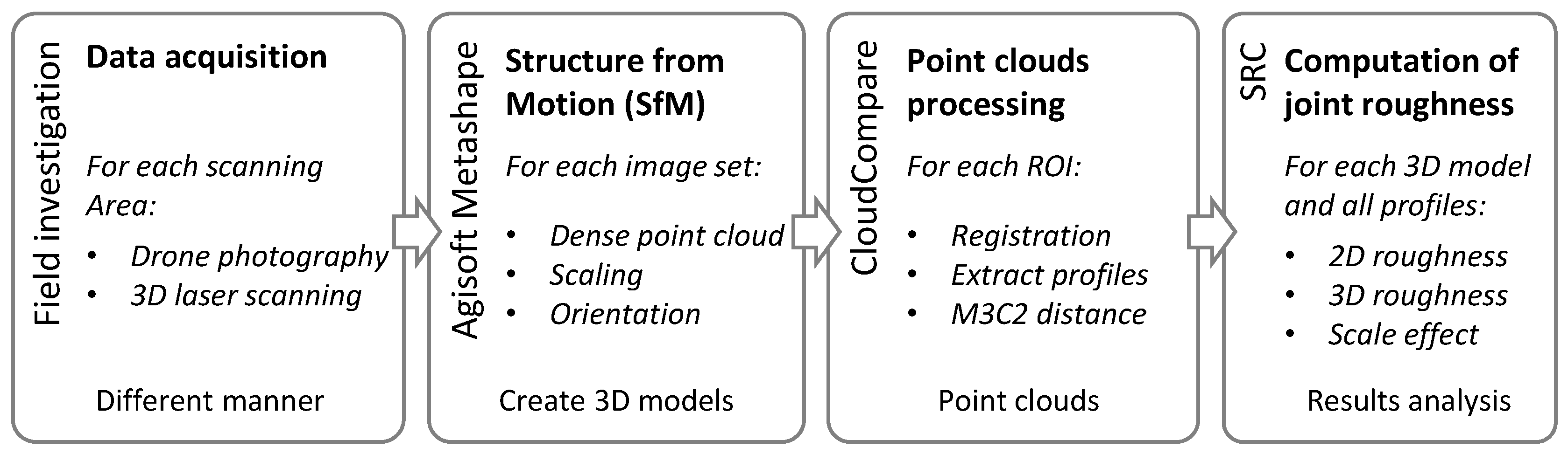
2. Materials and Methods
The proposed methodology primarily entails the following procedures: (1) Selecting a large-scale rock joint on a bench slope in the Lanping open pit mine located in Yunnan Province, China, as the target for measurement; (2) performing 3D reconstruction of the aforementioned large-scale joint surface using drone photogrammetry, which encompasses image capture and point cloud reconstruction; (3) employing a 3D laser scanner to scan the joint surface, generating a point cloud that serves as reference data with which to verify the applicability and accuracy of the drone photogrammetry; and (4) employing cloud-to-cloud distance and several roughness parameters as quantitative indicators in order to conduct a comparative analysis between the results obtained through drone photogrammetry and the laser scanner (Figure 1).
2.1. Description of the Joint Surface
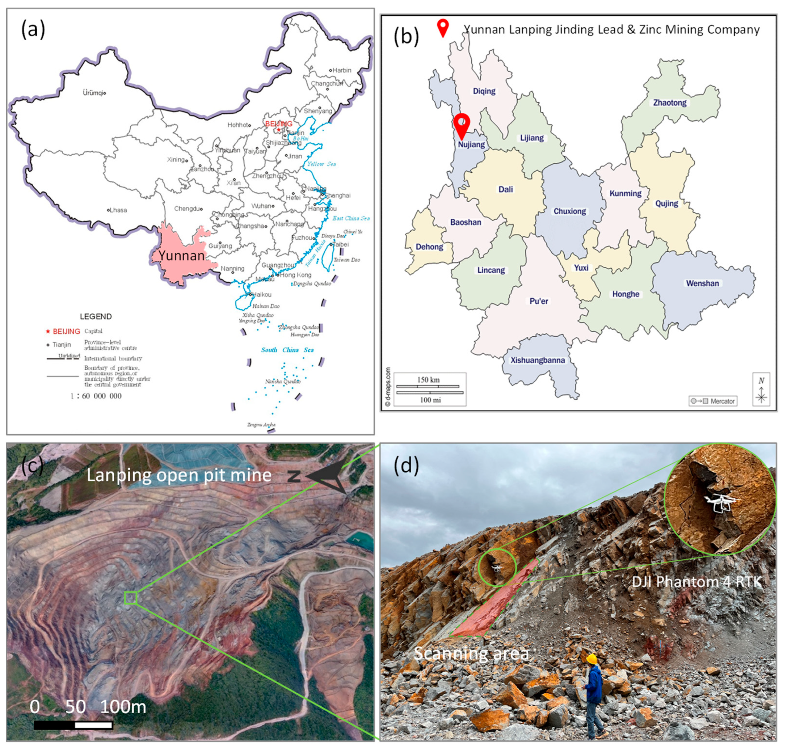
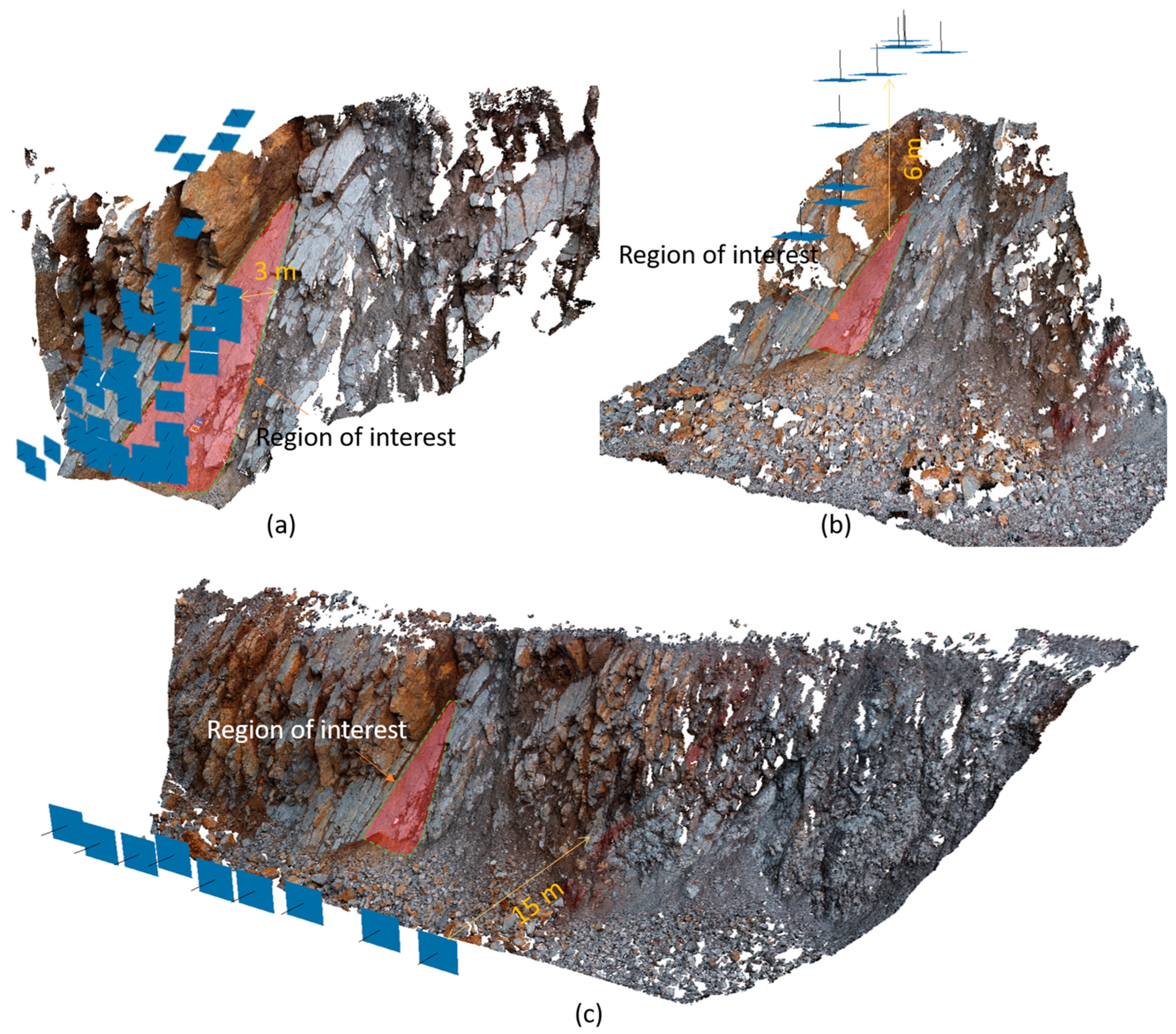
The Lanping open pit mine in Lanping County, Nujiang Lisu Autonomous Prefecture, Yunnan Province, China, is the largest confirmed lead-zinc deposit in the country, earning it the title of “Asia’s premier lead-zinc mine” (Figure 2a,b). The stratigraphic rock formations at this open pit mine comprise mainly Jurassic purplish-red sandy mudstone, Triassic greyish-black mudstone, Cretaceous calcareous sandstone, and Tertiary Yunlong formation argillaceous sandstone. The surveyed joint surfaces in this mining area are located on the southern slope, exhibiting a grey-white calcareous quartz sandstone lithology that corresponds to the dip direction of the main joint surfaces developed within the rock layers (Figure 2c). We selected a well-exposed, clean-surfaced, impurity-free joint surface measuring approximately 6.0 m × 2.0 m with which to investigate the potential of using drone photogrammetry for roughness measurements (Figure 2d).
This joint surface belongs to an interbed fault zone, characterized by a relatively straight development that extends across the entire step slope. The slope potential failure mode is characterized by planar sliding, which suggests that the stability of the bench slope is significantly influenced by the roughness of the joint surface. In order to effectively assess the stability of the slope and determine the appropriate parameters for estimating its shear strength, it is crucial to gain a comprehensive understanding of the roughness properties exhibited by the surface of the joints.
2.2. Point Clouds Generated with Drone Photogrammetry
2.2.1. Image Capture
In this study, a DJI Phantom 4 RTK drone—an unmanned aerial vehicle designed for professional surveying and mapping—was employed to capture joint surface images. The drone is equipped with a high-precision GNSS module for centimeter-level positioning accuracy and a 20 MP camera for high-quality image capture. Additionally, it features a time sync system for accurate timestamping and a flight autonomy system to ensure safe, stable flight. The drone can be operated manually via remote control or programmed to follow a predetermined route using planning software. Hence, this drone is ideal for slope investigation. In this study, we chose manual flight mode for safety reasons, as the joint surface to be investigated was small compared to the overall size of the slope, and the terrain was highly variable.
Based on the general rules for image photography, in order to ensure sufficient overlap between images to provide enough data for 3D model reconstruction, a minimum overlap of 60% is needed for photogrammetry [34]. We strictly followed this guideline during the image acquisition process, controlling the drone to move slowly in order to ensure that the overlap between two adjacent photos was greater than 60%. In addition, in order to assess the impact of shooting distance on photogrammetry modelling results, we took three sets of photographs at different distances and angles. The first set of photographs was taken about 3 m away from the joint surface, in a direction approximately perpendicular to the joint surface. In the second set of photos, the camera shot the joint surface vertically downward, at an average distance of about 6 m. The last set of photographs was taken horizontally, about 15 m from the joint surface.
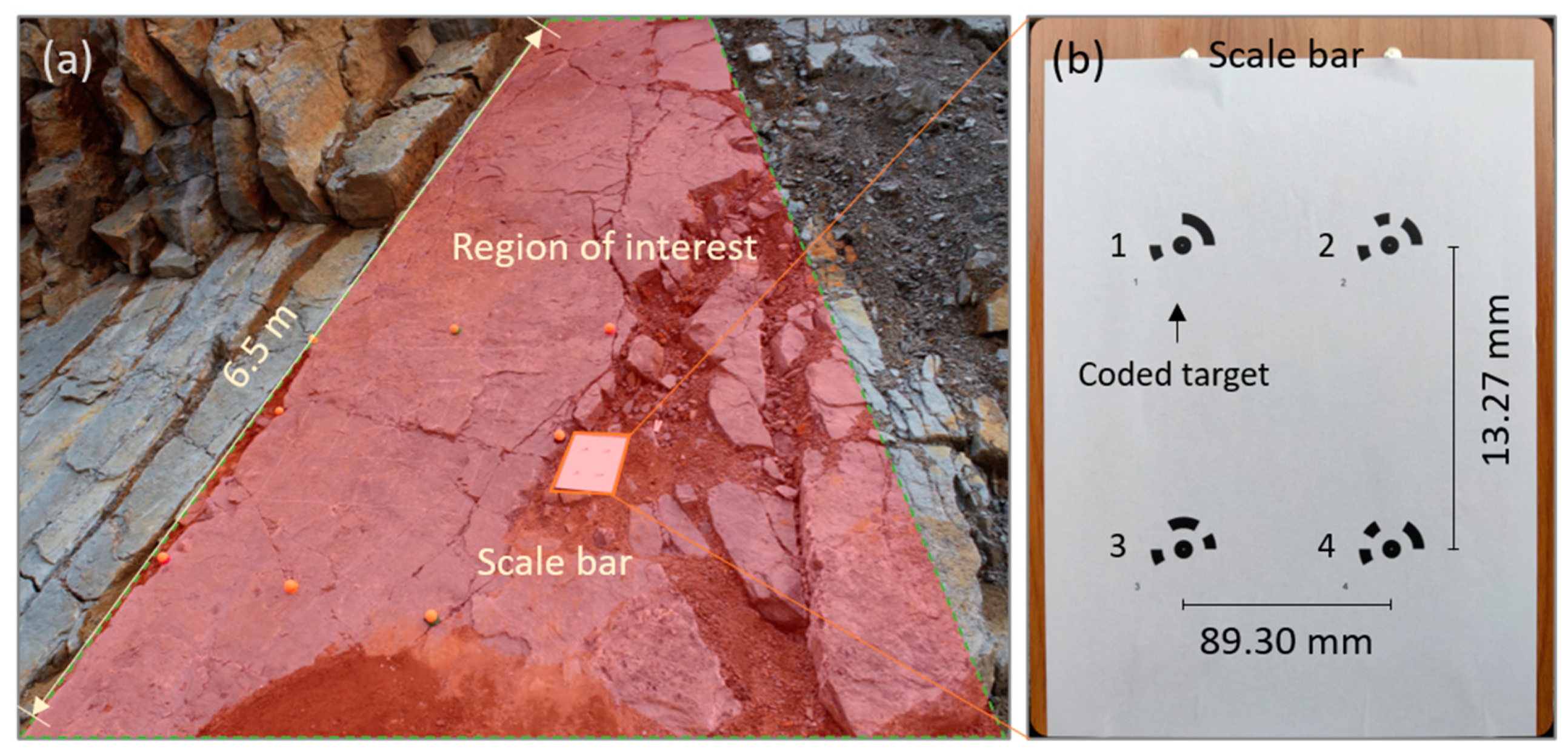
The inclusion of an RTK module in the DJI Phantom 4 RTK drone enables high-precision positioning information and significantly reduces the need for ground control points (GCPs). This significantly reduces the workload of field measurements, thereby enhancing work efficiency. Considering the high precision requirements for measuring joint surface roughness, we made a scale bar as an auxiliary tool with which to calibrate the resulting three-dimensional model. The scale bar was constructed by printing four coded targets on A4 paper and subsequently pasting them onto a wooden board. The distances between adjacent coded targets are known (Figure 3).
Another crucial factor that influences the results of outdoor photogrammetry is light [35]. In order to minimize the adverse effects of cloud cover and direct sunlight on the photography process, we chose to schedule our shooting session immediately after sunset. This specific timeframe allows for a low position of the sun in the sky, resulting in gently diffused and inviting illumination. Consequently, this approach aided in mitigating the presence of harsh shadows and enhancing the overall caliber of the captured visuals.
2.2.2. Point Cloud Reconstruction
Structure from Motion (SfM) is a widely employed photogrammetric methodology that facilitates the creation of 3D models through the utilization of a sequence of 2D images that possess overlapping features [36]. The SfM algorithm initiates by making estimations of the camera’s position and orientation for each image it has captured. The process of achieving this involves the identification of shared characteristics, such as corners or edges, within the images, followed by the establishment of correspondences between these characteristics across multiple images. Following this, the algorithm employs the identified features and makes estimations of the camera poses within a 3D space. Agisoft Metashape (Version 1.5.1) is widely recognized as a prevalent software application utilized for conducting SfM photogrammetry and producing 3D model reconstructions. This software’s popularity can be attributed to its intuitive user interface, sophisticated algorithms, and ability to work with diverse data formats. The software exhibits the capability to generate accurate and comprehensive 3D models derived from a collection of input images, rendering it appropriate for a diverse array of applications encompassing architecture, archaeology, topographic mapping, and so on [37,38,39,40].
The operation of Agisoft Metashape software is straightforward, requiring only a few steps to obtain a detailed 3D model. Firstly, the acquired images are imported into the software. Next, the photos are aligned to identify common features and estimate camera positions. This step generates a sparse point cloud, representing the rough 3D structure of the scene. Subsequently, a dense point cloud is built to refine the model, increasing the number of points and improving accuracy. Since the experiment only requires a dense point cloud model, processes such as building a mesh, a tiled model, or a digital elevation model are unnecessary. During the alignment and dense point cloud construction, various settings and parameters can be adjusted to optimize the quality and precision of the 3D reconstruction. The adjustment of processing accuracy may have a significant effect on the outcome of the point cloud. In this study, using a computer equipped with an Intel Core i5-8500 CPU, 16 GB of RAM and an Nvidia GeForce GTX 1060 graphics card, we tested the software’s five provided options: lowest, low, moderate, high, and very high. The resulting point clouds generated by drone photogrammetry are referred to as the DP models. To assess the impact of image capturing mode and processing accuracy on the accuracy of joint surface roughness measurement, we conducted experiments involving three different shooting distances, five levels of processing precision, and three varied shooting directions. The test conditions including shooting distance, processing accuracy, and shooting direction are summarized in Table 1. The purpose of this test is to offer enhanced guidance for the utilization of drone photogrammetry in measuring joint surface roughness.
2.3. Point Clouds Acquired with Laser Scanning
The 3D laser scanner is widely recognized as a high-accuracy measuring instrument employed to capture 3D models of objects. In this study, a 3D laser scanner KSCAN-Magic-II manufactured by the Scantech company in Hangzhou, China was used to obtain the topography of the joint surface. The device’s resolution is 0.01 mm, and its volumetric accuracy can reach 0.03 mm/m. Therefore, the device has sufficient accuracy as a reference benchmark against which to evaluate the performance of drone photogrammetry.
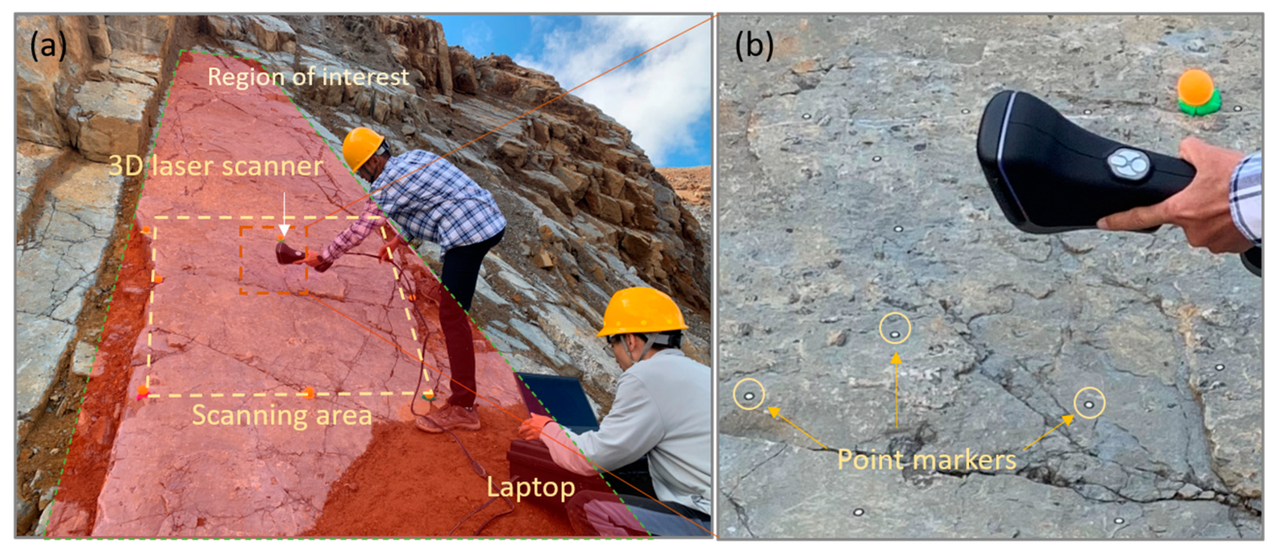
Due to the inaccessibility of the joint surface on the upper slope for scanning, we chose a smaller area measuring approximately 1.0 m × 1.0 m near the bottom of the slope (see Figure 4a). According to the device usage guide, it is necessary to affix markers to the object to aid in data registration and georeferencing. Here, we used point markers with a 5 mm diameter and spaced at intervals of approximately 10 cm on the joint surface (see Figure 4b). As a result, at least four markers were present within each scanning view. To create a detailed point cloud model of the joint surface without an excessive amount of data needed, we set the scanning sample interval to 0.5 mm. During scanning, the scanner was moved slowly and steadily across the rock joint surface, maintaining a consistent distance of approximately 0.3 m to 0.5 m. The collected point cloud information was transmitted in real-time to a laptop. Another individual reviewed the data, identified any areas of model defects, and instructed the scanner to perform additional scans until a complete 3D point cloud model of the joint was obtained. The resulting point cloud is referred to as the LS model.
2.4. Comparison between Laser Scanning and Drone Photogrammetry
2.4.1. Point Cloud Processing and 2D Profile Extraction
Point clouds, whether obtained from drone photogrammetry or the laser scanner, cannot be directly applied to roughness calculations. This is because of the potential inclusion of noise, outliers, and holes in these point clouds, which can affect the accuracy and quality of the model. Therefore, it is imperative to conduct the post-processing of point cloud data.
The first step in post-processing is the removal of outliers, which often requires manual deletion through careful observation. The second step involves filling the holes formed during the laser scanning process when the markers are attached to the joint surface, causing them to become holes. In this case, the “fill hole” command in Geomagic Studio 2014 is used to mend the point cloud model. The third step involves cropping the point cloud model to the area of interest. During the image capturing or laser scanning process, the software captures more information than just the area of interest, such as surrounding objects or the ground. Consequently, a point cloud model larger than the intended area of interest may be obtained. For calculation and comparison purposes, it is necessary to crop the point cloud model to the area of interest. In this study, we chose to crop the point cloud to an area of 1.0 m × 1.0 m. The fourth step involves point cloud resampling. It is well known that various roughness parameters are sensitive to the sampling interval of the point cloud model. Therefore, to perform a comparative analysis, we needed to resample both the laser scanning point cloud and the photogrammetry point cloud to a uniform sampling interval. In this study, we resampled the point spacing for each point cloud to 1.0 mm, 2.0 mm, 5.0 mm, and 10.0 mm. Therefore, each original point cloud would derive four point cloud models with different point spacing.
At present, the use of 2D profiles to quantify the roughness of joint surfaces is still a common method employed by most researchers. Therefore, we needed to extract the 2D profile from the 3D point cloud model for roughness calculation. This is the general workflow: First, perform a unified rotation and levelling treatment on all point cloud models to ensure that the joint surface lies within the XY plane. Next, define a plane that intersects the area of the point cloud. Subsequently, project the points within the selected area onto the defined plane to create a 2D representation of the point cloud. Finally, utilize a custom-made MATLAB plugin to vector the extracted profiles into equidistant numerical form for convenient calculations.
2.4.2. Point Cloud Comparison
The quality assessment of point cloud models generated via drone photogrammetry involved the utilization of the multiscale model-to-model cloud comparison (M3C2) algorithm. This algorithm computes the distance between the DP model and the LS model, aiming to evaluate differences between the two point clouds. Employing a locally estimated normal direction derived from the local surface roughness, the M3C2 algorithm effectively addresses uncertainties in point positions and registration errors. Furthermore, this algorithm operates at multiple scales using a normal-based projection, allowing for adaptability and effectiveness across different applications [41].
In this study, the open-source software CloudCompare (Version 2.12) was employed to compute the point cloud distances. Initially, all point clouds were imported into the software. Subsequently, the LS model was designated as the reference object, while the DP model was designated as the test object. The alignment tool was utilized to select multiple pairs of corresponding points in each cloud, in order to register them. The coordinate transformation matrix of the DP model was computed, thereby achieving a unified coordinate system for both the DP model and the LS model. Subsequently, utilizing the built-in M3C2 toolbox in the software, the distances between the point clouds were computed. This process involved several parameters, including the normal scale D, the projection scale d, and the projection depth h, which were determined via the GUESS functionality. Lastly, by means of statistical analysis, the minimum, maximum, mean, and standard deviation of the distance differences between the DP model and the LS model were determined.
2.4.3. Joint Roughness Estimation
Different roughness parameters characterize joint roughness from different perspectives [42,43]. To provide a comprehensive analysis, four 2D roughness parameters (Z1, Ai, Z2, PSD_D) and one 3D roughness parameter () were utilized to assess the roughness of the rock joint obtained from drone photogrammetry and 3D laser scanning. All of the roughness parameters mentioned above were calculated using the Surface Roughness Calculator (SRC) developed by Grasselli’s Geotechnics Group [43].
The root mean square of height (Z1) is a commonly used measure of joint roughness, as it provides a quantitative measure of the magnitude of microtopography fluctuations. The formula for calculating Z1 is:
where h1, h2 … hi are the height values, and i is the total number of height values.
The average asperity inclination (Ai) is a measure of the average angle of asperities (small irregularities) on a surface relative to a reference plane. This provides a measure of the overall orientation of the asperities on the surface. The formula for calculating Ai is as follows:
where L is total length of the profile, and hi is the profile height.
The root mean square slope (Z2) is a measure of the average inclination. This parameter is popular and useful for JRC estimation. The formula for calculating Z2 can be mathematically described as follows:
where L and h are the length and height of the profile, respectively.
The power spectral density (PSD), denoted with the symbol G(f), is a mathematical function that describes the distribution of power or energy of a profile over a range of frequencies. This allows for distinguishing the relative importance of waviness and unevenness. The calculation formula is presented below:
where D is the fractal dimension, λ0 represents the largest wavelength, and b is the crossover length.
is a popularly used 3D roughness parameter in joint roughness characterization created by Tatone and Grasselli (2009) [44]. The idea behind this approach is to discretize the joint surface into a finite number of triangles. The geometric orientations of these triangles are calculated. During shear tests, only the triangular units facing the direction of the shear contribute to the resistance to shear. The potential contact area is determined by the apparent dip angle, expressed as follows:
where represents the area normalized along the direction of analysis, represents the maximal apparent dip angle, and C represents the fitting parameter.
Root mean square error (RMSE) is a commonly used statistical measure of the difference between predicted values and actual values in a set of data. Here, the data obtained from the LS model are treated as actual values, and the data obtained from the drone photogrammetry are treated as predicted values. In this study, the measurement error ratio (Re) can be utilized to evaluate the performance of drone photogrammetry in measuring joint roughness. It is defined as follows:
where RoughnessLS and RoughnessDP represent the joint roughness derived from the laser scanner and drone photogrammetry, respectively; m represents the number of specimens.
3. Results
3.1. Point Clouds Generated with Drone Photogrammetry
A total of seven point cloud models were generated using drone photogrammetry. Figure 5 shows three of these models, which were captured at distances of 3 m, 6 m, and 15 m, respectively, with ultrahigh processing accuracy. The remaining four point cloud models had appearances similar to the model captured at a distance of 3 m, with the only difference being that different processing qualities were used. Upon careful inspection, we found that the joint surfaces of the area of interest were correctly reconstructed in terms of morphology, size, and spatial orientation. Although the drone’s attitude and position were controlled manually during the photo acquisition process, the good performance results for the reconstructions prove the stability and ease of use of UAV photogrammetry technology. Additionally, as shown in Figure 5, the size of the generated models increased as the capture distance increased. This is because more information outside of the area of interest was captured in the photos when the shooting distance was greater.
Table 2 summarizes the attributes of the point cloud models generated using drone photogrammetry and LS, including the number of photos, average ground sample distance, processing quality, tie point, dense point cloud, processing time, and nominal point spacing. When the capturing distance increased from 3 m to 15 m, the average ground sample distance increased from 1.1 mm/pixel to 4.8 mm/pixel. Such an increase can result in an inability to accurately identify small textures on the joint surface, thereby reducing the level of detail in the model. Additionally, modelling using different processing qualities can cause a huge difference in the number of points. The number of points ranges from 492,329 for the DP-3-lowest model to 131,175,925 for the DP-3-ultrahigh model, a difference of approximately 266 times, with a processing time increase of 58 times.
The LS model comprised a total of 5,273,602 points, with a nominal point spacing of 0.43 mm. Here, the nominal point spacing was obtained by dividing the number of points by the projected area of the joint surface and ignoring the undulation changes in the joint surface. Therefore, the nominal point spacing was smaller than the actual sampling spacing. Among all of the DP models, the DP-3-ultrahigh model had the smallest nominal point spacing of 0.92 mm. The nominal point spacings of the DP-6-ultrahigh and DP-15-ultrahigh models were 2.47 mm and 3.9 mm, respectively. It should be noted that the nominal point spacing only represents the number of points contained in the model, with more points indicating a higher level of detail in the model, but this does not indicate the accuracy of the model’s size or shape. In order to further examine the accuracy of the DP models, we utilized the M3C2 distance between the DP models and the LS model as a means to demonstrate their accuracy.
3.2. Cloud-to-Cloud Distance
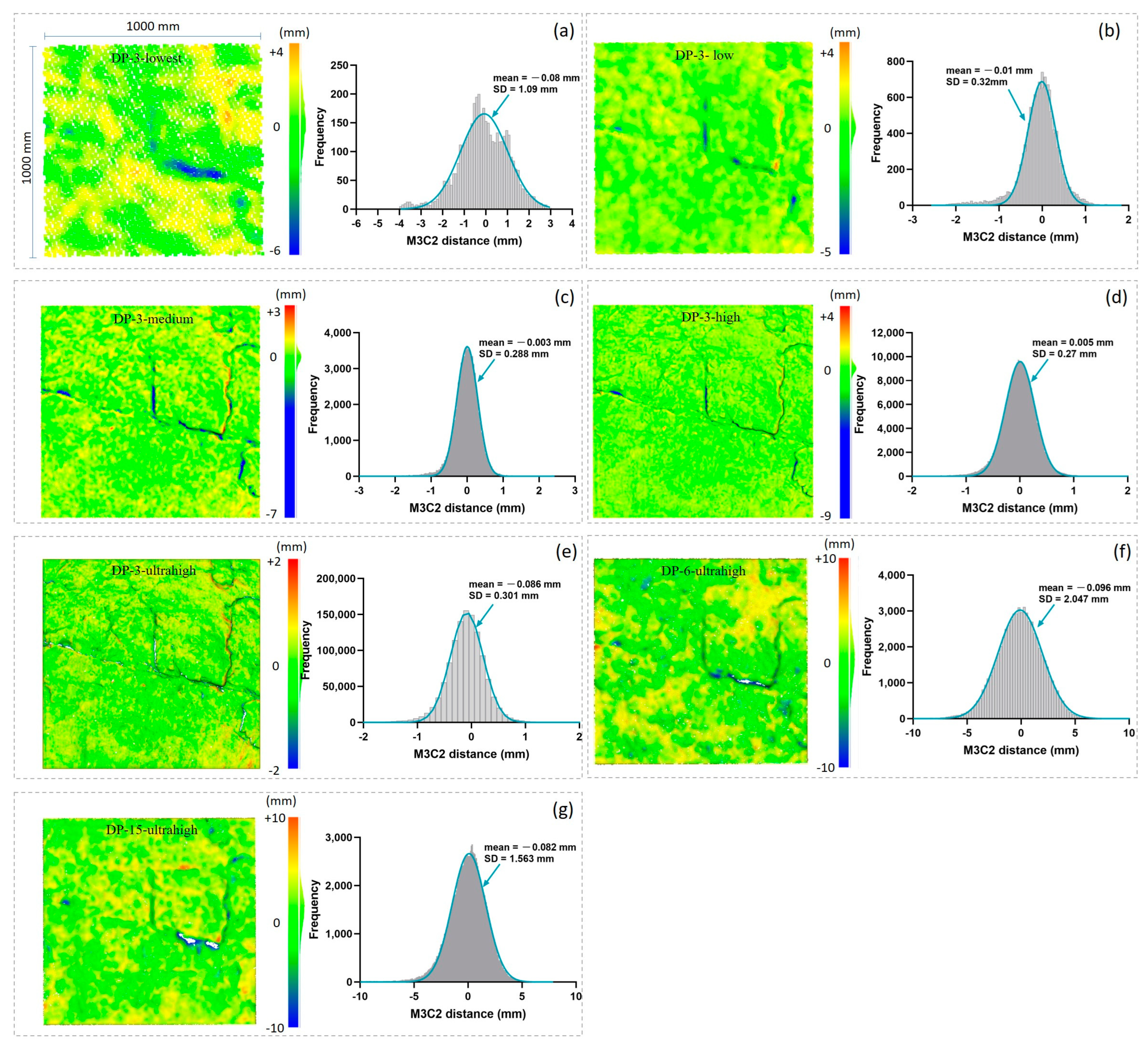
Figure 6 shows the distribution of M3C2 distances between the DP models and the LS model. According to the color in the figure, areas with larger M3C2 distance values are concentrated where the surface of the joint has larger height variations, while areas with relatively gentle slopes generally have smaller M3C2 distances. Furthermore, Table 3 provides a statistical analysis of the M3C2 distances of each model, including frequency, mean, standard deviation, and RMSE. Frequency represents the number of projection areas used in the computation, and this value controls the size of the “windows” used to compute the height differences between the two point clouds. In this practice, the choice of frequency value depended on the density of the point clouds being compared. The standard deviation represents the degree of dispersion of the M3C2 distances. The smaller this value, the more concentrated the M3C2 distance values. The accuracy of the DP models obtained through drone photogrammetry was evaluated using the root mean square error (RMSE) of the M3C2 distance, as defined in the accuracy standards set by the American Society for Photogrammetry and Remote Sensing (2015) [45].
For the five sets of DP models captured at a distance of 3 m, except for the DP-3-lowest model with an RMSE value of 1.16 mm, the RMSE values were between 0.4 mm and 0.5 mm. Combined with Table 2, this indicates that processing accuracy only has a significant impact on the level of detail in the model reconstruction, but has little effect on the geometric accuracy of the model. When the capture distances increased to 6 m and 15 m, the corresponding RMSE values of the models were 1.9 mm and 2.3 mm, respectively. Based on the author’s previous research, when reconstructing a joint surface using smartphone photogrammetry at a distance of 30 cm, the RMSE result obtained was approximately 0.05 mm. Therefore, we can roughly conclude that the accuracy of the DP models is positively correlated with the capture distance.
3.3. Measurement Error of Drone Photogrammetry
3.3.1. Measurement Error in 2D Profiles
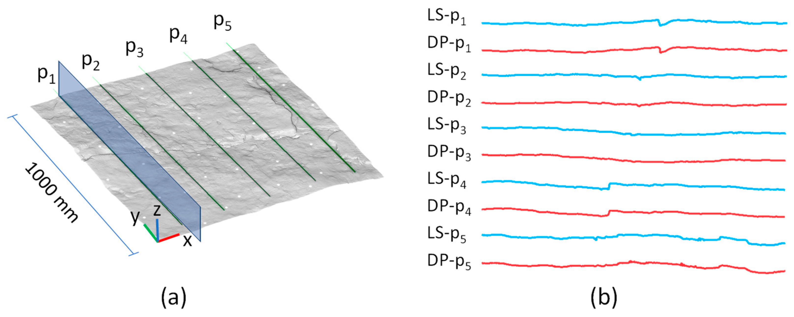
As shown in Figure 7, we extracted 2D profiles parallel to the YZ plane at five different locations in both the LS and DP models. Each point cloud model generated five profiles. Due to the influence of the number of dense point clouds, the profiles obtained from the DP-3-ultrahigh model were most similar to those obtained from the LS model, while the profiles obtained from the other models did not provide enough detail on the roughness features of the joint. Therefore, the profiles extracted from the DP-3-ultrahigh model were selected for comparison with the LS model. We named the five profiles obtained from the DP-3-ultrahigh model DP-p1, DP-p2, DP-p3, DP-p4, and DP-p5, and the five profiles obtained from the LS model LS-p1, LS-p2, LS-p3, LS-p4, and LS-p5.
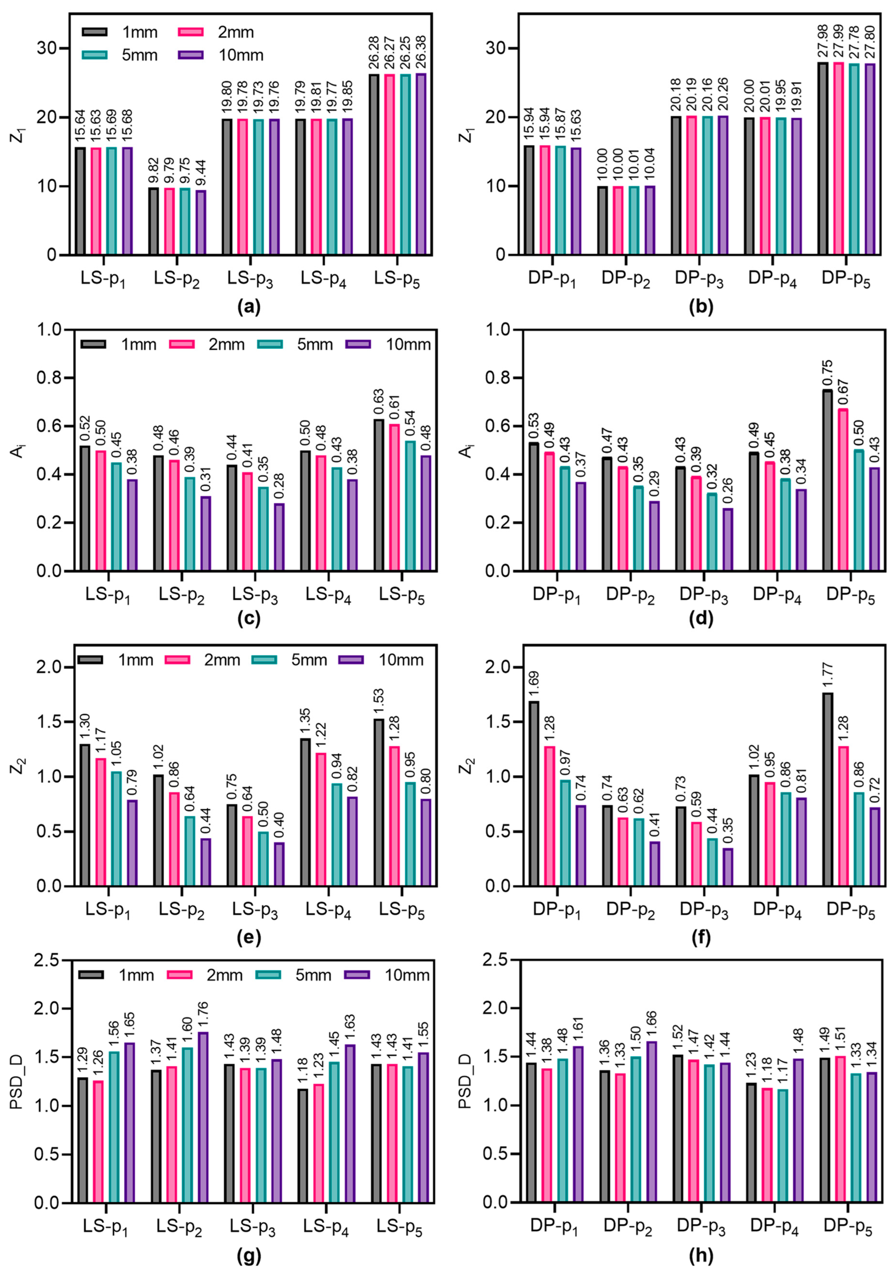
Considering the influence of sampling intervals on the roughness calculation results, this study used a linear interpolation technique in order to resample the extracted profiles, so that each original profile formed four profiles with point intervals of 1 mm, 2 mm, 5 mm, and 10 mm, respectively. Figure 8 lists the roughness values corresponding to profiles with different sampling intervals. The roughness parameters Z1 and PSD-D did not exhibit consistent changes with varying point intervals among the profiles, while the parameters Ai and Z2 decreased with increasing sampling intervals. This can be explained by the fact that both Ai and Z2 are parameters that describe the surface inclination angle of the joint surface. Increasing the sampling interval will make the profile smoother, thus reducing the values of Ai and Z2.
Additionally, using different roughness parameters to compare the roughness of two sets of joint surfaces may lead to conflicting conclusions, since different parameters represent distinct shape features of the profile. For example, the Z1 values of profiles LS-p3 and LS-p4 at a sampling interval of 1 mm were 19.80 and 19.79, respectively, indicating that their roughness was approximately the same. However, their corresponding Z2 values were 0.75 and 1.25, respectively, indicating that the roughness of LS-p4 was significantly greater than that of LS-p3. This shows that it is very important to specify the roughness parameters used when analyzing the roughness of a joint surface.
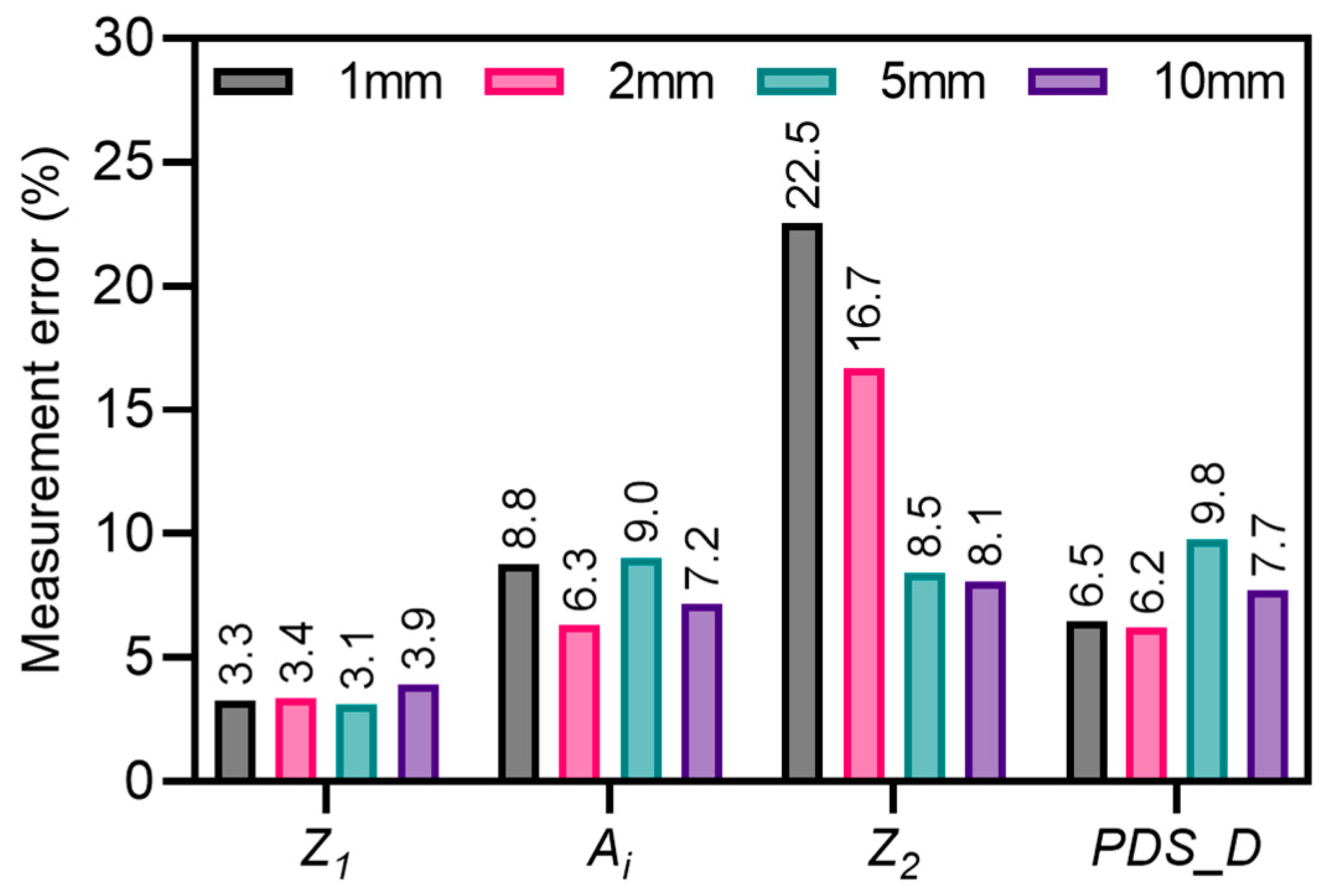
Furthermore, we calculated the measurement error of drone photogrammetry under different 2D roughness parameters according to Equation (5). The results indicate that the measurement errors of parameters Z1, Ai, and PSD-D were uncorrelated with the point spacing, and the average errors were 3.4%, 7.8%, and 7.6%, respectively. The measurement error of parameter Z2 was negatively correlated with the point spacing, with an error of 22.5% when the point spacing was 1 mm and an error of 8.1% when the point spacing was 10 mm (see Figure 9).
3.3.2. Measurement Error in 3D Surfaces
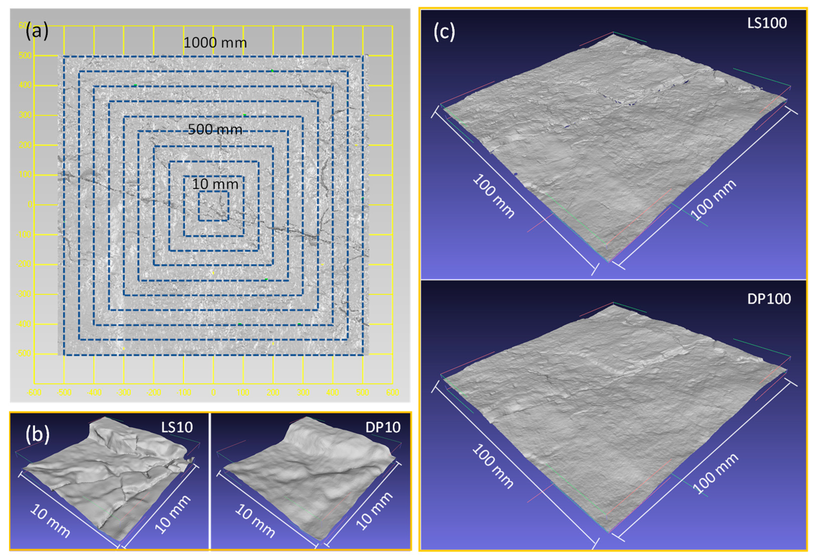
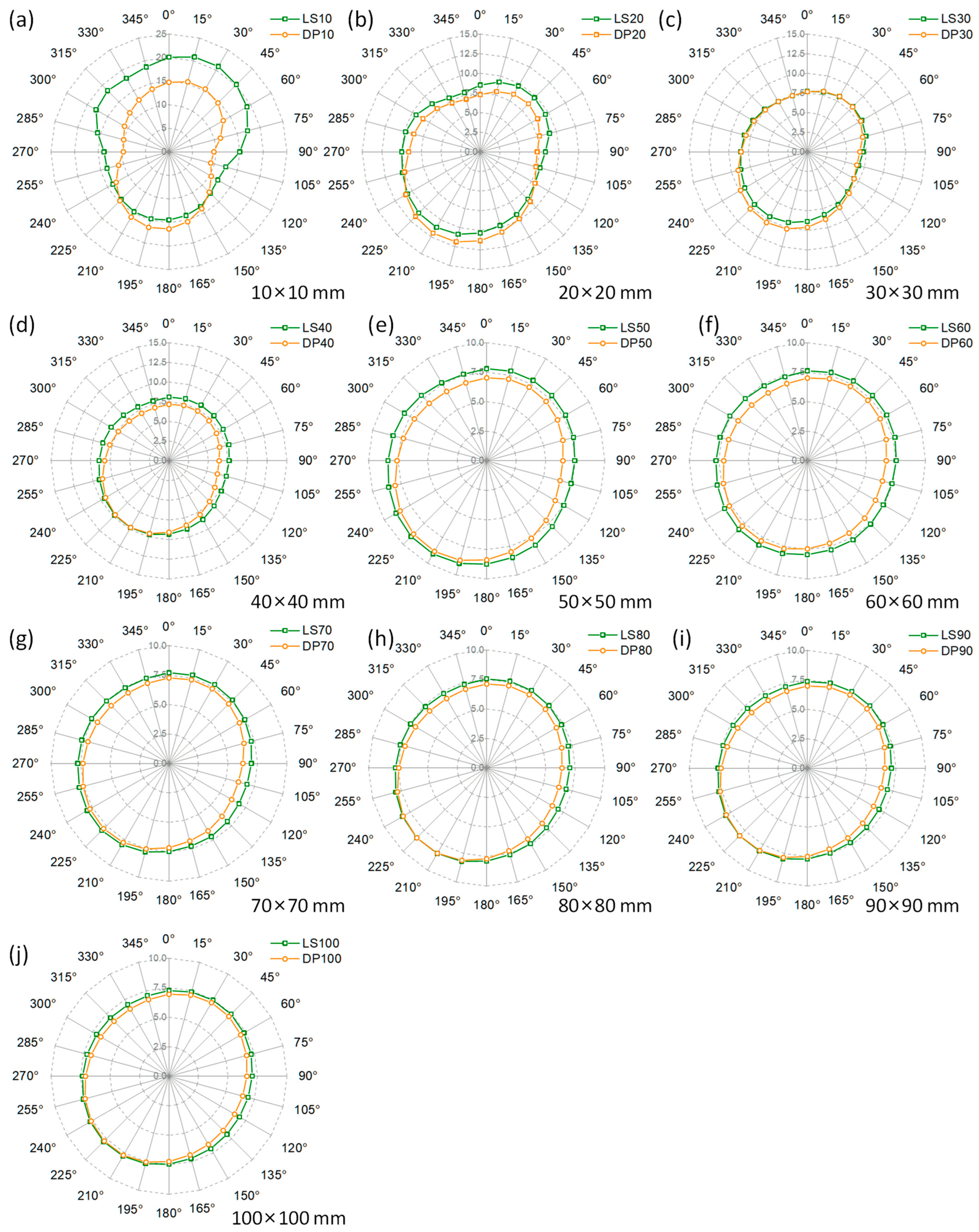
In order to comprehensively evaluate the accuracy and applicability of drone photogrammetry in measuring the 3D roughness of joint surfaces, this study used the central enlargement method to divide the point cloud models into 10 different sizes, ranging from 10 cm × 10 cm to 100 cm × 100 cm, for 3D roughness calculation (as shown in Figure 10). Figure 11 displays the 3D roughness of joint surfaces, varying in size and direction. The green line represents the results of the LS model, and the orange line represents the results of the DP model. When the sample size was 10 cm × 10 cm, there was significant deviation between the DP model and the LS model, with a maximum difference of approximately 5. As the model size increased, the results for the DP model and the LS model became more consistent with each other. Generally, the DP model yielded slightly smaller values compared to those of the LS model. In addition, it can be found that the joint roughness had significant anisotropy (Figure 11a), with a roughness value of 20 in the direction of about 30°, while the roughness value in the direction of 120° was 13. As the model size increased, the anisotropy of the model roughness gradually weakened (as shown in Figure 11b–j).
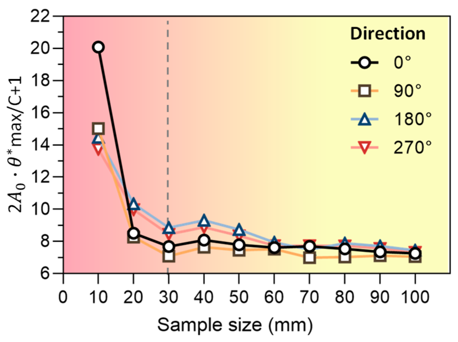
Numerous studies have shown that the roughness of joint surfaces has a size effect. Figure 12 shows the changes in the roughness of the LS model in four directions (0°, 90°, 180°, and 270°) with the variation in sample size. It can be observed that the roughness of this joint surface has a significant size effect, and when the sample size is larger than 30 cm × 30 cm, the roughness value tends to stabilize, indicating that the roughness size threshold of this joint surface is about 30 cm × 30 cm.
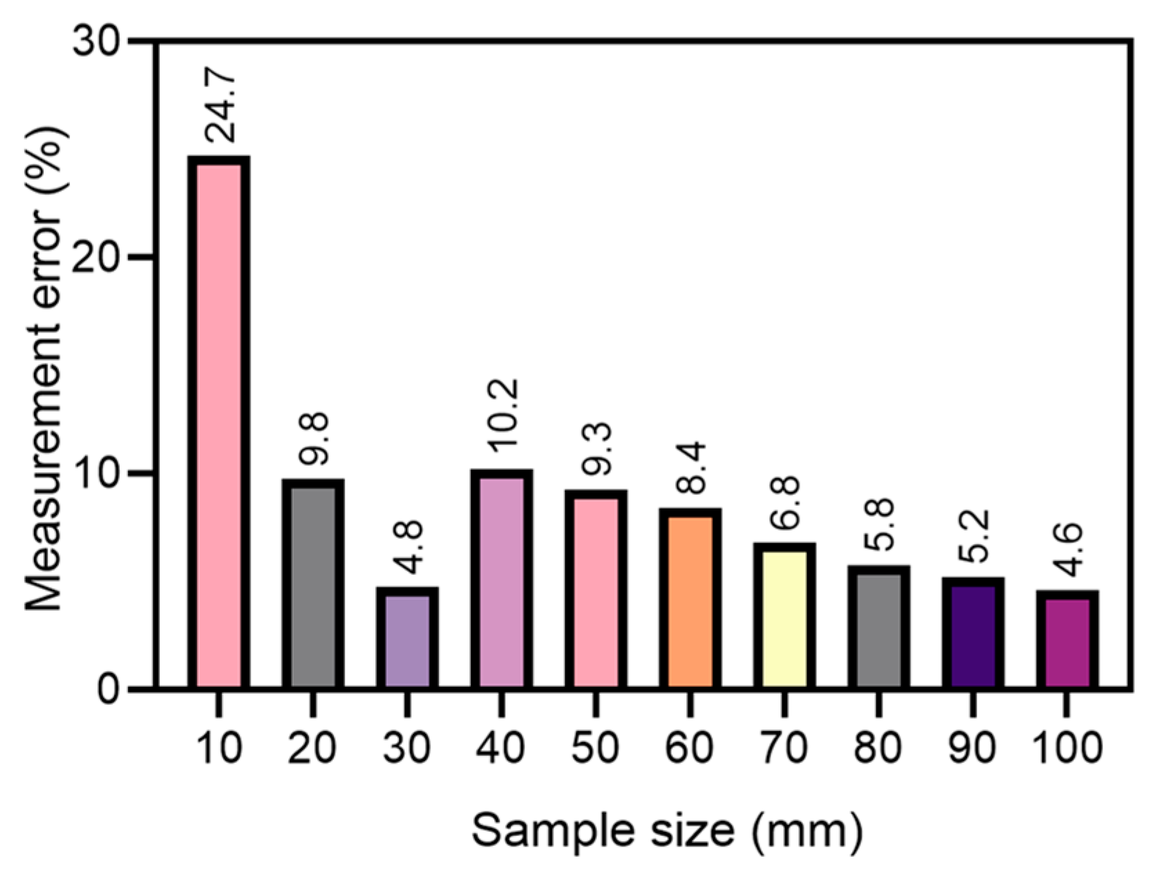
Figure 13 illustrates the measurement errors of 3D roughness for DP models with different sizes. For the joint size of 10 cm × 10 cm, the measurement error was 24.7%. As the joint size exceeded 20 cm × 20 cm, the measurement error decreased sharply and generally did not exceed 10%. When the size of the joint surface was 100 cm × 100 cm, the measurement error reached a minimum of 4.6%. These results are consistent with the measurement errors observed in 2D roughness and affirm that drone photogrammetry is a reliable and practical tool for measuring the roughness of joint surfaces.
4. Discussion
4.1. How Accurate Is Accurate Enough in Joint Roughness Measurement?
The measurement accuracy of joint surface topography is a very important issue, but it seems to have received little attention and discussion in the literature. When Barton first proposed the JRC concept, the profiler used was made up of flat stainless steel metal shims, approximately 3 per mm [46]. Many researchers have since used pin-type profilometers purchased from hardware stores, with rod diameters of about 1 mm [25]. Du (1992) designed a proposed longitudinal profile instrument that continuously draws the undulating contour of the joint surface using a plotting pen, thus avoiding the problem of sampling resolution [16]. Regarding the application of non-contact measurement methods in indoor joint surface measurement, the ISRM recommends that the measurement precision of the equipment should be better than 0.025 mm [47]. In addition, the accuracy of laser scanners used by various researchers varies, and is also related to the measurement distance. Researchers seem to assume that the accuracy of their measurement equipment is sufficient, and have developed various empirical formulas for the shear strength of joint surfaces based on this assumption. However, there is currently no standard answer or criterion for the level of accuracy measurement the equipment needs to achieve in order to meet the requirements of joint surface roughness measurement.
Our research findings indicate that different roughness parameters exhibit varying sensitivities to the morphology of the joint surface. Parameters Z1 and Ai display insensitivity to the sampling interval, with a deviation of only approximately 5%, compared to the values obtained from 3D laser scanning. Conversely, parameter Z2 demonstrates sensitivity to the sampling interval, resulting in significant variation in results across different sampling intervals. The results demonstrate that the accuracy level necessary for joint roughness measurements depends on the intended data application. In large-scale field assessments of joint surface roughness, demanding the same accuracy level as that required for small-scale surfaces may prove challenging and impractical. Consequently, we propose establishing an error tolerance range, correlated with the joint surface size, for various measurement situations. This approach would ensure that measurement results maintain adequate accuracy for their intended purpose while considering the practical constraints of the equipment and techniques employed.
4.2. Challenges and Considerations in Drone Photogrammetry
Based on our experimental findings, drone photogrammetry yields highly accurate measurements and offers the advantages of efficiency and cost-effectiveness. Consequently, it is an exceptional approach for conducting roughness surveys on steep and hazardous slopes, where conventional measurement methods may pose implementation challenges or safety risks. However, it is crucial to consider the challenges and constraints associated with this methodology. These include factors such as weather conditions, environmental circumstances, data collection strategies, restricted resolution, and processing time [48]. The effectiveness of drone photogrammetry is significantly influenced by prevailing weather patterns and environmental factors. Adverse weather conditions, such as strong winds and rain, can affect the execution of measurement tasks. In regions without network connectivity, the use of RTK drones additionally requires terrestrial base stations for accurate positioning. This requirement increases the complexity and financial burden of the operation, as additional equipment and personnel become necessary. Additionally, transparent minerals or high reflectivity on certain rock surfaces can cause distortions in measurements [49]. Therefore, when using drone photogrammetry to quantify the roughness of joint surfaces, it is imperative to conduct thorough investigations in order to ensure the precision and reliability of the measurement outcomes. This may involve visually examining the joint surface for potential sources of error, selecting appropriate camera parameters and lighting conditions to minimize the impact of reflectivity, and using specialized software and algorithms to correct any distortions in the measurement data.
Data collection strategies play a crucial role in UAV photogrammetry, as they directly impact the accuracy and reliability of the obtained results [50]. In this study, we discovered that a 3.0 m distance and positioning the camera perpendicular to the joint surface can lead to a good result. However, it is important to note that this strategy may not be optimal, and further comprehensive testing is required. One key aspect of data collection is planning the drone flight, which involves determining optimal flight parameters such as altitude, overlap, and sidelap [51]. These parameters directly influence the resolution and quality of the captured images, subsequently affecting the accuracy of the resulting point cloud and orthomosaic. Consistency in image capture is also critical during data collection. It is imperative to maintain a steady flight path, avoid sudden maneuvers, and consider environmental conditions such as wind and lighting. Overall, the use of effective data collection strategies in drone photogrammetry is vital for obtaining accurate, reliable, and high-quality results. By carefully planning and executing the measurement process, it is possible to guarantee the accuracy and reliability of the results, even in complex measurement scenarios.
4.3. Point Cloud Postprocessing and Roughness Estimation
This study required the utilization of Agisoft Metashape, CloudCompare, Geomagic Studio 2014, and SRC to generate a point cloud model and perform roughness calculations. Nevertheless, the utilization of such software tools can pose difficulties and consume significant amounts of time for individuals lacking familiarity with software operations, thereby potentially impeding the extensive implementation of this technology. The need for prompt decision-making and effective response based upon on-site investigations often necessitates the utilization of expedited data processing and analysis. The potential for simplifying the processing and analysis of field survey data exists with the advent of cloud-based processing systems. The process involves the field investigators uploading the photographs they have gathered to a server. Subsequently, a cloud-based system promptly undertakes the task of processing and analyzing the data to ascertain the roughness of the seam surface [52]. By adopting this approach, scholars in the respective domain will not require the utilization of specialized software or hardware, thereby resulting in cost reduction and enhanced technology usability.
5. Conclusions
This study evaluated the accuracy of drone photogrammetry technology for measuring large-scale rock joint roughness under field conditions. A handheld laser scanner was used as a benchmark against which to compare with the results obtained from drone photogrammetry. In order to provide a comprehensive comparison and analysis, four different 2D roughness parameters and one 3D roughness parameter were employed to characterize the roughness of the joint surface. Additionally, the influence factors, including point spacing and scale effect, were investigated. The following are the main conclusions of this study:
- The M3C2 distances between models generated using drone photogrammetry and laser scanning show that the shooting distance is the primary factor influencing the accuracy of drone photogrammetry. Under a 3 m image capture distance using drone photogrammetry, the root mean square error of M3C2 distance is less than 0.5 mm. The processing quality in Agisoft Metashape, rather than the surface morphology, primarily impacts the level of detail in the resulting model.
- The measurement error of drone photogrammetry for most roughness parameters does not exceed 10%. For the 2D roughness parameters Z1, Ai, and PSD-D were 3.4%, 7.8%, and 7.6%, respectively. The measurement error of parameter Z2 is negatively correlated with the point spacing, with an error of 22.5% at a point spacing of 1.0 mm, and an error of 8.1% at a point spacing of 10.0 mm.
- The measurement error of drone photogrammetry for 3D roughness () decreases exponentially with increasing joint scale. For small joint surfaces measuring 10 cm × 10 cm, the error is 24.7%. However, for larger joint surfaces measuring 100 cm × 100 cm, the error decreases to around 4.6%.
In summary, this study demonstrated the feasibility and potential of drone photogrammetry for joint roughness measurement challenges. With this technology, we can obtain accurate and detailed measurements of the roughness of joint surfaces that can be used to improve our understanding of the mechanical behavior of rock masses and to design safe and stable engineering structures. However, accuracy, limitations and practical considerations need to be taken into account for real-world applications.
Author Contributions
Conceptualization, P.A.; methodology, J.S.; software, J.S. and P.A.; validation, J.S., and P.A.; investigation, S.D., R.Y., C.W. and P.A.; resources, S.D.; data curation, P.A.; writing—original draft preparation, J.S. and P.A.; writing—review and editing, R.Y. and C.W. visualization, J.S.; supervision, S.D.; project administration, S.D.; funding acquisition, S.D. and R.Y. All authors have read and agreed to the published version of the manuscript.
Funding
The research was funded by the National Natural Science Foundation of China (Nos. 42177117, 41427802, and 41572299), Zhejiang Provincial Natural Science Foundation (No. LQ16D020001), Zhejiang Collaborative Innovation Center for Prevention and Control of Mountain Geological Hazards (Nos. PCMGH-2017-Z03, PCMGH-2017-Y-04, and PCMGH-2017-Y-05), and Ningbo Natural Science Foundation (Grant No. 2023J084).
Data Availability Statement
Data available upon request to corresponding author.
Conflicts of Interest
The authors declare no conflict of interest.
References
- Kwasniewski, M.A.; Wang, J.-A. Surface Roughness Evolution and Mechanical Behavior of Rock Joints under Shear. Int. J. Rock Mech. Min. Sci. 1997, 34, 709. [Google Scholar]
- Belem, T.; Souley, M.; Homand, F. Modeling Surface Roughness Degradation of Rock Joint Wall during Monotonic and Cyclic Shearing. Acta Geotech. 2007, 2, 227–248. [Google Scholar]
- Barton, N.; Wang, C.; Yong, R. Advances in Joint Roughness Coefficient (JRC) and Its Engineering Applications. J. Rock Mech. Geotech. Eng. 2023. [Google Scholar] [CrossRef]
- Wu, Q.; Kulatilake, P.H.S.W. REV and Its Properties on Fracture System and Mechanical Properties, and an Orthotropic Constitutive Model for a Jointed Rock Mass in a Dam Site in China. Comput. Geotech. 2012, 43, 124–142. [Google Scholar] [CrossRef]
- Wu, Q.; Liu, Y.; Tang, H.; Kang, J.; Wang, L.; Li, C.; Wang, D.; Liu, Z. Experimental Study of the Influence of Wetting and Drying Cycles on the Strength of Intact Rock Samples from a Red Stratum in the Three Gorges Reservoir Area. Eng. Geol. 2023, 314, 107013. [Google Scholar] [CrossRef]
- Guo, S.; Qi, S. Numerical Study on Progressive Failure of Hard Rock Samples with an Unfilled Undulate Joint. Eng. Geol. 2015, 193, 173–182. [Google Scholar] [CrossRef]
- Park, J.-W.; Song, J.-J. Numerical Method for the Determination of Contact Areas of a Rock Joint under Normal and Shear Loads. Int. J. Rock Mech. Min. Sci. 2013, 58, 8–22. [Google Scholar] [CrossRef]
- Wang, C.; Wang, H.; Qin, W.; Wei, S.; Tian, H.; Fang, K. Behaviour of Pile-Anchor Reinforced Landslides under Varying Water Level, Rainfall, and Thrust Load: Insight from Physical Modelling. Eng. Geol. 2023, 325, 107293. [Google Scholar] [CrossRef]
- Tatone, B.S. Quantitative Characterization of Natural Rock Discontinuity Roughness In-Situ and in the Laboratory; University of Toronto: Toronto, ON, Canada, 2009. [Google Scholar]
- Morelli, G.L. On Joint Roughness: Measurements and Use in Rock Mass Characterization. Geotech. Geol. Eng. 2014, 32, 345–362. [Google Scholar] [CrossRef]
- Kulatilake, P.H.S.W.; Ankah, M.L.Y. Rock Joint Roughness Measurement and Quantification—A Review of the Current Status. Geotechnics 2023, 3, 116–141. [Google Scholar] [CrossRef]
- Stimpson, B. A Rapid Field Method for Recording Joint Roughness Profiles. In Proceedings of the International Journal of Rock Mechanics and Mining Sciences & Geomechanics Abstracts; Pergamon: Oxford, UK, 1982; Volume 19, pp. 345–346. Available online: https://www.sciencedirect.com/science/article/abs/pii/0148906282913699?via%3Dihub (accessed on 18 September 2023).
- Weissbach, G. A New Method for the Determination of the Roughness of Rock Joints in the Laboratory. Int. J. Rock Mech. Min. Sci. 1978, 15. [Google Scholar] [CrossRef]
- Maerz, N.H.; Franklin, J.A.; Bennett, C.P. Joint Roughness Measurement Using Shadow Profilometry. Int. J. Rock Mech. Min. Sci. Geomech. Abstr. 1990, 27, 329–343. [Google Scholar] [CrossRef]
- Wang, C.; Yong, R.; Luo, Z.; Du, S.; Karakus, M.; Huang, C. A Novel Method for Determining the Three-Dimensional Roughness of Rock Joints Based on Profile Slices. Rock Mech. Rock Eng. 2023. [Google Scholar] [CrossRef]
- Du, S. Simple profile instrument and its application on studying joint roughness coefficient of rock. Geol. Sci. Technol. Inf. 1992, 11, 91–95. [Google Scholar]
- Mah, J.; Samson, C.; McKinnon, S.D.; Thibodeau, D. 3D Laser Imaging for Surface Roughness Analysis. Int. J. Rock Mech. Min. Sci. 2013, 58, 111–117. [Google Scholar] [CrossRef]
- Marsch, K.; Wujanz, D.; Fernandez-Steeger, T.M. On the Usability of Different Optical Measuring Techniques for Joint Roughness Evaluation. Bull. Eng. Geol. Environ. 2020, 79, 811–830. [Google Scholar] [CrossRef]
- Li, B.; Mo, Y.; Zou, L.; Wu, F. An Extended Hyperbolic Closure Model for Unmated Granite Fractures Subject to Normal Loading. Rock Mech. Rock Eng. 2022, 55, 4139–4158. [Google Scholar] [CrossRef]
- Khoshelham, K.; Altundag, D.; Ngan-Tillard, D.; Menenti, M. Influence of Range Measurement Noise on Roughness Characterization of Rock Surfaces Using Terrestrial Laser Scanning. Int. J. Rock Mech. Min. Sci. 2011, 48, 1215–1223. [Google Scholar] [CrossRef]
- Jiang, Q.; Feng, X.; Gong, Y.; Song, L.; Ran, S.; Cui, J. Reverse Modelling of Natural Rock Joints Using 3D Scanning and 3D Printing. Comput. Geotech. 2016, 73, 210–220. [Google Scholar] [CrossRef]
- García-Luna, R. Characterization of Joint Roughness Using Spectral Frequencies and Photogrammetric Techniques. BGM 2020, 131, 445–458. [Google Scholar] [CrossRef]
- García-Luna, R.; Senent, S.; Jimenez, R. Using Telephoto Lens to Characterize Rock Surface Roughness in SfM Models. Rock Mech. Rock Eng. 2021, 54, 2369–2382. [Google Scholar] [CrossRef]
- Paixão, A.; Muralha, J.; Resende, R.; Fortunato, E. Close-Range Photogrammetry for 3D Rock Joint Roughness Evaluation. Rock Mech. Rock Eng. 2022, 55, 3213–3233. [Google Scholar] [CrossRef]
- Kim, D.H.; Poropat, G.; Gratchev, I.; Balasubramaniam, A. Assessment of the Accuracy of Close Distance Photogrammetric JRC Data. Rock Mech. Rock Eng. 2016, 49, 4285–4301. [Google Scholar]
- Zhao, L.; Huang, D.; Chen, J.; Wang, X.; Luo, W.; Zhu, Z.; Li, D.; Zuo, S. A Practical Photogrammetric Workflow in the Field for the Construction of a 3D Rock Joint Surface Database. Eng. Geol. 2020, 279, 105878. [Google Scholar] [CrossRef]
- An, P.; Fang, K.; Jiang, Q.; Zhang, H.; Zhang, Y. Measurement of Rock Joint Surfaces by Using Smartphone Structure from Motion (SfM) Photogrammetry. Sensors 2021, 21, 922. [Google Scholar] [CrossRef]
- An, P.; Fang, K.; Zhang, Y.; Jiang, Y.; Yang, Y. Assessment of the Trueness and Precision of Smartphone Photogrammetry for Rock Joint Roughness Measurement. Measurement 2022, 188, 110598. [Google Scholar] [CrossRef]
- Zhang, F.; Hassanzadeh, A.; Kikkert, J.; Pethybridge, S.J.; van Aardt, J. Comparison of UAS-Based Structure-from-Motion and LiDAR for Structural Characterization of Short Broadacre Crops. Remote Sens. 2021, 13, 3975. [Google Scholar] [CrossRef]
- Battulwar, R.; Winkelmaier, G.; Valencia, J.; Naghadehi, M.Z.; Peik, B.; Abbasi, B.; Parvin, B.; Sattarvand, J. A Practical Methodology for Generating High-Resolution 3D Models of Open-Pit Slopes Using UAVs: Flight Path Planning and Optimization. Remote Sens. 2020, 12, 2283. [Google Scholar] [CrossRef]
- Cheng, Z.; Gong, W.; Tang, H.; Juang, C.H.; Deng, Q.; Chen, J.; Ye, X. UAV Photogrammetry-Based Remote Sensing and Preliminary Assessment of the Behavior of a Landslide in Guizhou, China. Eng. Geol. 2021, 289, 106172. [Google Scholar] [CrossRef]
- Salvini, R.; Vanneschi, C.; Coggan, J.S.; Mastrorocco, G. Evaluation of the Use of UAV Photogrammetry for Rock Discontinuity Roughness Characterization. Rock Mech. Rock Eng. 2020, 53, 3699–3720. [Google Scholar] [CrossRef]
- García-Luna, R.; Senent, S.; Jimenez, R. Characterization of Joint Roughness Using Close-Range UAV-SfM Photogrammetry. IOP Conf. Ser. Earth Environ. Sci. 2021, 833, 012064. [Google Scholar] [CrossRef]
- Jiménez-Jiménez, S.I.; Ojeda-Bustamante, W.; Marcial-Pablo, M.d.J.; Enciso, J. Digital Terrain Models Generated with Low-Cost UAV Photogrammetry: Methodology and Accuracy. ISPRS Int. J. Geo-Inf. 2021, 10, 285. [Google Scholar] [CrossRef]
- Bruno, N.; Giacomini, A.; Roncella, R.; Thoeni, K. Influence of illumination changes on image-based 3D surface reconstruction. Int. Arch. Photogramm. Remote Sens. Spat. Inf. Sci. 2021, 43, 701–708. [Google Scholar] [CrossRef]
- Luhmann, T.; Robson, S.; Kyle, S.; Boehm, J. Close-Range Photogrammetry and 3D Imaging; Walter de Gruyter: Berlin, Germany, 2013; ISBN 3-11-030278-0. [Google Scholar]
- Taddia, Y.; González-García, L.; Zambello, E.; Pellegrinelli, A. Quality Assessment of Photogrammetric Models for Façade and Building Reconstruction Using DJI Phantom 4 RTK. Remote Sens. 2020, 12, 3144. [Google Scholar] [CrossRef]
- Fang, K.; An, P.; Tang, H.; Tu, J.; Jia, S.; Miao, M.; Dong, A. Application of a Multi-Smartphone Measurement System in Slope Model Tests. Eng. Geol. 2021, 295, 106424. [Google Scholar] [CrossRef]
- An, P.; Tang, H.; Li, C.; Fang, K.; Lu, S.; Zhang, J. A Fast and Practical Method for Determining Particle Size and Shape by Using Smartphone Photogrammetry. Measurement 2022, 193, 110943. [Google Scholar] [CrossRef]
- Fang, K.; Zhang, J.; Tang, H.; Hu, X.; Yuan, H.; Wang, X.; An, P.; Ding, B. A Quick and Low-Cost Smartphone Photogrammetry Method for Obtaining 3D Particle Size and Shape. Eng. Geol. 2023, 322, 107170. [Google Scholar] [CrossRef]
- Lague, D.; Brodu, N.; Leroux, J. Accurate 3D Comparison of Complex Topography with Terrestrial Laser Scanner: Application to the Rangitikei Canyon (NZ). ISPRS J. Photogramm. Remote Sens. 2013, 82, 10–26. [Google Scholar]
- Belem, T.; Homand-Etienne, F.; Souley, M. Quantitative Parameters for Rock Joint Surface Roughness. Rock Mech. Rock Eng. 2000, 33, 217–242. [Google Scholar] [CrossRef]
- Magsipoc, E.; Zhao, Q.; Grasselli, G. 2D and 3D Roughness Characterization. Rock Mech. Rock Eng. 2020, 53, 1495–1519. [Google Scholar] [CrossRef]
- Tatone, B.S.A.; Grasselli, G. A Method to Evaluate the Three-Dimensional Roughness of Fracture Surfaces in Brittle Geomaterials. Rev. Sci. Instrum. 2009, 80, 125110. [Google Scholar] [CrossRef] [PubMed]
- American Society for Photogrammetry. Remote Sensing ASPRS Positional Accuracy Standards for Digital Geospatial Data. Photogramm. Eng. Remote Sens. 2015, 81, 1–26. [Google Scholar] [CrossRef]
- Barton, N.; Choubey, V. The Shear Strength of Rock Joints in Theory and Practice. Rock Mech. 1977, 10, 1–54. [Google Scholar] [CrossRef]
- Muralha, J.; Grasselli, G.; Tatone, B.; Blümel, M.; Chryssanthakis, P.; Yujing, J. ISRM Suggested Method for Laboratory Determination of the Shear Strength of Rock Joints: Revised Version. In The ISRM Suggested Methods for Rock Characterization, Testing and Monitoring: 2007–2014; Ulusay, R., Ed.; Springer International Publishing: Cham, Switzerland, 2014; pp. 131–142. ISBN 978-3-319-07713-0. [Google Scholar]
- Eltner, A.; Kaiser, A.; Castillo, C.; Rock, G.; Neugirg, F.; Abellán, A. Image-Based Surface Reconstruction in Geomorphometry-Merits, Limits and Developments. Earth Surf. Dyn. 2016, 4, 359–389. [Google Scholar]
- Hosseininaveh Ahmadabadian, A.; Karami, A.; Yazdan, R. An Automatic 3D Reconstruction System for Texture-Less Objects. Robot. Auton. Syst. 2019, 117, 29–39. [Google Scholar] [CrossRef]
- Dai, W.; Zheng, G.; Antoniazza, G.; Zhao, F.; Chen, K.; Lu, W.; Lane, S.N. Improving UAV-SfM Photogrammetry for Modelling High-Relief Terrain: Image Collection Strategies and Ground Control Quantity. Earth Surf. Process. Landf. 2023. [Google Scholar] [CrossRef]
- James, M.R.; Chandler, J.H.; Eltner, A.; Fraser, C.; Miller, P.E.; Mills, J.P.; Noble, T.; Robson, S.; Lane, S.N. Guidelines on the Use of Structure-from-motion Photogrammetry in Geomorphic Research. Earth Surf. Process. Landf. 2019, 44, 2081–2084. [Google Scholar] [CrossRef]
- Barbero-García, I.; Lerma, J.L.; Mora-Navarro, G. Fully Automatic Smartphone-Based Photogrammetric 3D Modelling of Infant’s Heads for Cranial Deformation Analysis. ISPRS J. Photogramm. Remote Sens. 2020, 166, 268–277. [Google Scholar] [CrossRef]
Figure 1.
Flowchart of the method proposed for determining rock joint roughness on a slope using drone photogrammetry.
Figure 1.
Flowchart of the method proposed for determining rock joint roughness on a slope using drone photogrammetry.

Figure 2.
Study area (a) location of Yunnan on a map of China, (b) location of the Lanping open pit mine in Yunnan province, (c) top view of the Lanping open pit mine, and (d) joint surfaces and sites in the process of study with drone photography.
Figure 2.
Study area (a) location of Yunnan on a map of China, (b) location of the Lanping open pit mine in Yunnan province, (c) top view of the Lanping open pit mine, and (d) joint surfaces and sites in the process of study with drone photography.

Figure 3.
Scale bar, (a) the scale bar placed at the region of interest and (b) the distance between two adjacent coded targets. The horizontal distance is 89.30 mm, and the vertical distance is 13.27 mm.
Figure 3.
Scale bar, (a) the scale bar placed at the region of interest and (b) the distance between two adjacent coded targets. The horizontal distance is 89.30 mm, and the vertical distance is 13.27 mm.

Figure 4.
Point cloud acquisition using a 3D laser scanner, (a) scanning process, and (b) point markers fixed on the joint surface.
Figure 4.
Point cloud acquisition using a 3D laser scanner, (a) scanning process, and (b) point markers fixed on the joint surface.

Figure 5.
Point clouds generated using drone photogrammetry with different shooting distances: (a) 3 m, (b) 6 m, and (c) 15 m.
Figure 5.
Point clouds generated using drone photogrammetry with different shooting distances: (a) 3 m, (b) 6 m, and (c) 15 m.

Figure 6.
M3C2 distance between the DP model and LS model. (a–g) refer to models DP-3-lowest, DP-3-low, DP-3-medium, DP-3-high, DP-3-ultrahigh, DP-6-ultrahigh, and DP-15-ultrahigh, respectively.
Figure 6.
M3C2 distance between the DP model and LS model. (a–g) refer to models DP-3-lowest, DP-3-low, DP-3-medium, DP-3-high, DP-3-ultrahigh, DP-6-ultrahigh, and DP-15-ultrahigh, respectively.

Figure 7.
2D Profiles extracted from DP and LS models: (a) positions of the five profiles; (b) profiles of p1–p5.
Figure 7.
2D Profiles extracted from DP and LS models: (a) positions of the five profiles; (b) profiles of p1–p5.

Figure 8.
Roughness results for the 2D profiles with different sampling intervals and roughness parameters. (a,c,e,g) correspond to the LS profiles, while (b,d,f,h) correspond to the DP profiles.
Figure 8.
Roughness results for the 2D profiles with different sampling intervals and roughness parameters. (a,c,e,g) correspond to the LS profiles, while (b,d,f,h) correspond to the DP profiles.

Figure 9.
Joint roughness measurement error at different point spacings with drone photogrammetry.

Figure 10.
The point cloud model is cropped to different sizes using the center enlargement method. (a) The plane schematic diagram, wherein the blue dotted line signifies the cropped samples, and the yellow line represents the rectangular coordinates. (b) The point cloud model with a size of 10 cm × 10 cm, and (c) the point cloud model with a size of 100 cm × 100 cm.

Figure 11.
Results for 3D joint roughness from the LS models and DP models at different scales; (a–j) represent the different joint scales, ranging from 10 cm × 10 cm to 100 cm × 100 cm.
Figure 11.
Results for 3D joint roughness from the LS models and DP models at different scales; (a–j) represent the different joint scales, ranging from 10 cm × 10 cm to 100 cm × 100 cm.

Figure 12.
The effect of joint scale on the 3D roughness.

Figure 13.
3D roughness measurement error of drone photogrammetry in different joint surface sizes.


Table 1.
Image capturing scheme for reconstructing point clouds using drone photogrammetry.
| Equipment | Shooting | Processing | Shooting | Model No. |
|---|---|---|---|---|
| Distance (m) | Accuracy | Direction | ||
| Phantom 4 RTK | 3 | Lowest | Oblique | DP-3-lowest |
| Phantom 4 RTK | 3 | Low | Oblique | DP-3-low |
| Phantom 4 RTK | 3 | Medium | Oblique | DP-3-medium |
| Phantom 4 RTK | 3 | High | Oblique | DP-3-high |
| Phantom 4 RTK | 3 | Ultrahigh | Oblique | DP-3-ultrahigh |
| Phantom 4 RTK | 6 | Ultrahigh | Vertical | DP-5-ultrahigh |
| Phantom 4 RTK | 15 | Ultrahigh | Horizontal | DP-15-ultrahigh |
Table 2.
Basic information of the point clouds generated through drone photogrammetry and LS.
| Model No. | Number of Images | Average Ground Sample Distance (mm/pixel) | Processing Quality | Tie Point | Dense Point Cloud | PT * (seconds) | NPS ** (mm) |
|---|---|---|---|---|---|---|---|
| LS | - | - | - | - | 5,373,602 | - | 0.43 |
| DP-3-lowest | 53 | 1.1 | lowest | 6126 | 492,329 | 39 | 15.26 |
| DP-3-low | 53 | 1.1 | low | 30,298 | 2,023,343 | 82 | 7.52 |
| DP-3-medium | 53 | 1.1 | medium | 136,851 | 8,421,748 | 319 | 3.74 |
| DP-3-high | 53 | 1.1 | high | 220,947 | 33,241,996 | 1736 | 1.86 |
| DP-3-ultrahigh | 53 | 1.1 | ultrahigh | 198,687 | 131,175,924 | 2285 | 0.92 |
| DP-6-ultrahigh | 11 | 2.1 | ultrahigh | 9844 | 60,255,510 | 204 | 2.47 |
| DP-15-ultrahigh | 9 | 4.8 | ultrahigh | 11,713 | 63,331,233 | 155 | 3.90 |
* PT—processing time, ** NPS—nominal point spacing.
Table 3.
The M3C2 distances between the DP model and LS model.
| Model No. | M3C2 | RMSE (mm) | ||
|---|---|---|---|---|
| Frequency | Mean (mm) | Standard Deviation (mm) | ||
| DP-3-lowest | 4292 | −0.08 | 1.09 | 1.16 |
| DP-3-low | 17,685 | −0.01 | 0.32 | 0.46 |
| DP-3-medium | 71,440 | −0.003 | 0.288 | 0.44 |
| DP-3-high | 288,987 | 0.005 | 0.27 | 0.42 |
| DP-3-ultrahigh | 1,169,755 | −0.086 | 0.301 | 0.52 |
| DP-6-ultrahigh | 163,848 | −0.096 | 2.047 | 1.9 |
| DP-15-ultrahigh | 65,615 | −0.082 | 1.563 | 2.3 |
Disclaimer/Publisher’s Note: The statements, opinions and data contained in all publications are solely those of the individual author(s) and contributor(s) and not of MDPI and/or the editor(s). MDPI and/or the editor(s) disclaim responsibility for any injury to people or property resulting from any ideas, methods, instructions or products referred to in the content. |
© 2023 by the authors. Licensee MDPI, Basel, Switzerland. This article is an open access article distributed under the terms and conditions of the Creative Commons Attribution (CC BY) license (https://creativecommons.org/licenses/by/4.0/).
Share and Cite
MDPI and ACS Style
Song, J.; Du, S.; Yong, R.; Wang, C.; An, P. Drone Photogrammetry for Accurate and Efficient Rock Joint Roughness Assessment on Steep and Inaccessible Slopes. Remote Sens. 2023, 15, 4880. https://doi.org/10.3390/rs15194880
AMA Style
Song J, Du S, Yong R, Wang C, An P. Drone Photogrammetry for Accurate and Efficient Rock Joint Roughness Assessment on Steep and Inaccessible Slopes. Remote Sensing. 2023; 15(19):4880. https://doi.org/10.3390/rs15194880
Chicago/Turabian StyleSong, Jiamin, Shigui Du, Rui Yong, Changshuo Wang, and Pengju An. 2023. "Drone Photogrammetry for Accurate and Efficient Rock Joint Roughness Assessment on Steep and Inaccessible Slopes" Remote Sensing 15, no. 19: 4880. https://doi.org/10.3390/rs15194880
Note that from the first issue of 2016, this journal uses article numbers instead of page numbers. See further details here.