

Automated Determination of the Volume of Loose Engineering Deposits Using Terrestrial Laser Scanning
by
 ,
,
Bo Lu
1,
Jichen Zhu
2,
Yunfeng Ge
2,*,
Qian Chen
2,
Zhongxu Wen
2,
Geng Liu
2,3 and
Liangquan Li
4 1
Northwest Engineering Co., Ltd., PowerChina Corporation, Xi’an 710065, China
2
Faculty of Engineering, China University of Geosciences, Wuhan 430074, China
3
Hunan Earthquake Agency, Changsha 410004, China
4
Huadong Engineering Co., Ltd., PowerChina Corporation, Hangzhou 311122, China
*
Author to whom correspondence should be addressed.
Remote Sens. 2023, 15(18), 4604; https://doi.org/10.3390/rs15184604
Submission received: 15 June 2023
/
Revised: 14 August 2023
/
Accepted: 16 September 2023
/
Published: 19 September 2023
(This article belongs to the Section Remote Sensing in Geology, Geomorphology and Hydrology)
Abstract
:A new method for automatic volume determination of loose engineering deposits (LEDs) using point clouds collected by terrestrial laser scanning is proposed. The method starts with a problem of lacking bottom surface point clouds when scanning LEDs, assuming that the bottom surface is flat, a spatial plane is generated based on the plane fitting to the bottom surface. Then the sample point cloud is projected on this fitted plane to construct the subface point clouds, which, together with the initial point cloud data, are stitched into complete point cloud data with good closure, integrity, and accuracy. The 3D surface model established by introducing the alpha shape algorithm calculates the volume, and the validation experiments on three soil mound models and one field experiment on LEDs with a minimum average error of only 1.69% fully validate the effectiveness and accuracy of the method. The encouraging results show that effective volume calculation can be performed on realistic LEDs using the proposed method.
1. Introduction
Loose engineering deposits (LEDs) are typical unfavorable geological bodies that can easily undergo collapse, excessive deformation, and uneven settlement during engineering construction and even result in serious engineering disasters. Therefore, it is crucial to prevent engineering disasters during construction on loose deposits. The morphological study and volume calculation of LEDs has been a hot topic in engineering research, and its application area is wide. In large construction projects such as highways, railroads, tunnels, and ports, earthwork accounts for a large part of the total cost and requires a large amount of planning and continuous productivity assessment. The calculation of the volume of LEDs should be as accurate and efficient as possible, which is beneficial to cost control [1]. The volume of material transportation, use, and consumption can also be used as an indicator to predict the progress of the project [2]. In open pit mining and stripping projects, the stripping as well as mining works are large, and site managers need to know the approximate mineral reserves, as well as production and efficiency. The volume determination results are directly linked to economic interests and directly affect the arrangement of staff and equipment [3], which helps mines achieve their goals, while determining the amount of storage space required to provide a basis for pit backfill and land reclamation plans [4]. Land resources development and consolidation are effective measures to achieve the dynamic balance between the amount of arable land and the population, and the investment in earth movement for land leveling accounts for about 40% to 80% of the total investment. The accurate and efficient calculation of loose earth deposits is related to the investment in and effect of land resources development and consolidation to improve the quality of land use [5]. For natural geological hazards such as landslides, the accurate calculation of the volume size of the loose deposits of landslides that have already occurred helps in analyzing the extent of their causation and carrying out rescue work; the identification of potential landslide forms and the estimation of volumes help in early warning forecasting and the placement of engineering management measures [6,7]. Scheidegger (1977) argued that if the potential landslide volume can be estimated, the correlation between it and the friction coefficient can be used to predict the expected extent of sliding, and this correlation in the equation denotes the landslide volume and the friction coefficient [8]. Zhou et al. (2017) identified and analyzed the morphology of 12 typical landslides in the Martian Sailor Valley and studied the calculation scheme of the volume to derive the statistical laws between the volume of landslides and the area of the accumulation [9], and between the equivalent friction coefficient of landslides and the volume of landslides. This helped to better explain the mechanism of landslide formation and the interaction between landslides on Mars and the environment, as well as being important for the study of the reference value of landslides on Earth. Therefore, the volume calculation for LEDs, especially intelligent calculation, is of great importance in production.
Due to the different accumulation methods and different morphology of the LEDs, they are irregular geometries in space and there is no standard analytical formula for volume calculation. The commonly used traditional earth determination methods mainly include the square grid method, triangular grid method, section method, contour method, etc. Among them, the contour method measures the coordinates of discrete points on the surface of a LED by using a total station or real-time dynamic positioning (RTK), establishes a digital model of the deposit surface by drawing contour lines, and then calculates the volume of the deposit [10]. The traditional methods, however, are complicated by the shape of the deposit; uneven discrete determination points and local points cannot be measured, along with other factors [11,12], which greatly affect the efficiency and accuracy of volume determination of LED and bring inconvenience to the subsequent research. With the development of remote sensing technology, remote sensing images and a digital elevation model (DEM) are widely used, such as when McEwen used Mars Sailor Valley image data to estimate the volume of landslides in Sailor Valley and determined the calculation formula [13]. This scheme requires many experimental conditions, such as weather, ground cover, etc., resulting in the relatively low accuracy of the scheme, while remote sensing image classification and target identification still rely on manual work, which is less accurate and not efficient enough. More efficient and reliable data acquisition, as well as volume calculation methods, should be adopted.
Terrestrial laser scanning technology, a kind of remote sensing, has been widely used in many fields such as industry, art, and engineering in recent years as a new means of surveying and mapping [14]. The terrestrial laser scanner can acquire high-precision point clouds of the LEDs in a short period and accurately represent the surface characteristics of the measured object. Meanwhile, 3D laser scanning technology can collect data remotely without contact and measure locations that are inconvenient for staff to reach when working conditions are limited [15,16]. The 3D scanning technology was used for field determinations of architectural heritage to obtain real spatial data models of traditional ancient buildings, which provided reference data for the conservation and restoration of traditional buildings [17]. Liu et al. (2021) combined 3D laser scanning technology and BIM and reviewed various applications in the building life cycle [18]. In terms of morphology identification and volume determination of LEDs, Ge et al. (2020) utilized the point clouds of landslide deposits collected by terrestrial laser scanning to further identify and extract particles in the LED [19]. Yang et al. (2020) extracted and measured volume algorithms from 3D coal deposits by multi-scale directional curvature, which uses multiple grids and triangular prisms to reconstruct peak and slope points and calculate the volume of the deposit [3]. Lai et al. (2022) patched the 2.5D underwater point cloud acquired with 3D laser scanning and estimated the volume of underwater objects using the alpha shape algorithm [20]. Huising and Gomes Pereira (1998) estimated the error and accuracy of laser data acquired by various laser scanning systems used for terrain applications, and the results showed that laser scanning can be used for various purposes of terrain information extraction [21].
Several algorithms are available to generalize bounding polygons enveloping a set of points (point clouds), which is essential for constructing the 3D surface model of the LED. Among them, the alpha shape algorithm is a potential tool to address the abovementioned problems. Conceptually, the alpha shape is defined as the generalization of the polytope of a finite point set, which is uniquely determined by the point set and an alpha radius. For a given set of points, the alpha radius controls the fit level of the convex hull to the point set. Assume that a generalized disk or sphere with the alpha radius contains the points to produce the alpha shape. If the alpha radius = ∞, a convex hull will be created. If the alpha radius = 0, an empty alpha shape will be produced. If alpha radius = (0, ∞), it is possible to generate a non-convex region through tightening or loosening the fit around the points [22,23]. However, due to the inherent technical defects of the impenetrability of the laser scanning, it is impossible to collect the bottom boundary of the LED, resulting in the missing bottom point clouds of the LED. Correspondingly, it is difficult for researchers to determine the boundary conditions of the deposit, which in turn causes uncertainty in its volume calculation using the existing algorithms. Therefore, there is an urgent need for automatic and intelligent calculation methods with simple operation and accurate results in the volume calculation of LEDs.
This paper aims to propose a new method to automatically and accurately measure the volume of LEDs using point clouds collected by laser scanning. Using the terrestrial laser scanner, the 3D point clouds of deposits can be directly obtained, and most LEDs are placed on the ground in reality. Assuming that the bottom surface of the LED is flat-based, an algorithm was proposed to fit the bottom surface and construct a complete 3D point cloud with good closure, integrity, and accuracy. Finally, the alpha shape algorithm was introduced to convert the 3D point cloud into a closed geometry for the volume calculation of the LED.
2. Methodology
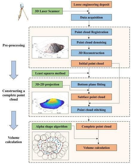
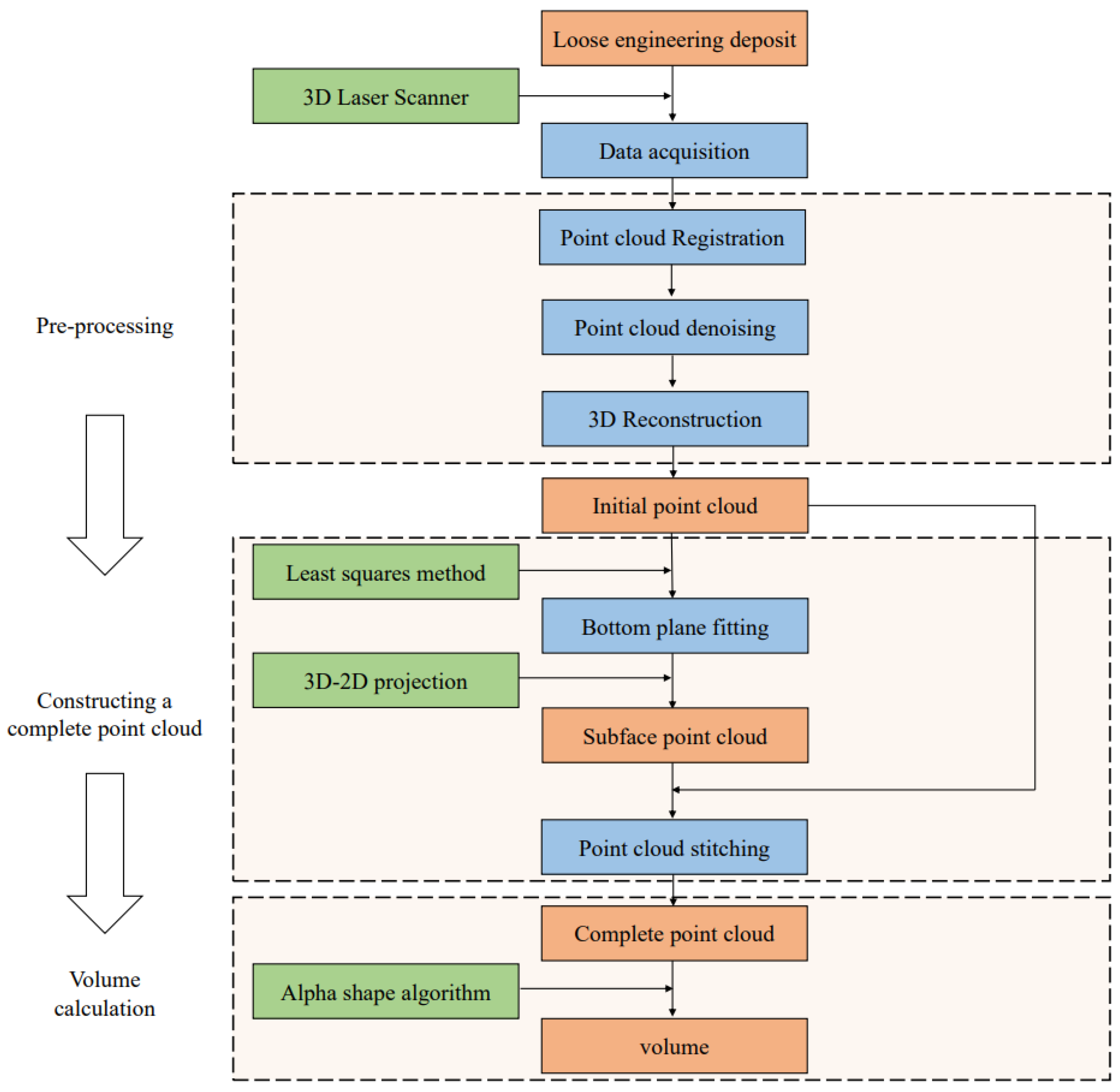
The flow chart of the main methodology of this study is shown in Figure 1. After determining the research targets, the 3D laser scanner is used for point cloud acquisition, and the volume determination mainly includes the following steps: point cloud pre-processing, complete point cloud construction, and volume calculation. The pre-processing process is assisted by Geomagic software, and the complete point cloud data construction and volume calculation process is realized automatically using the proposed algorithms. For more details, please see the subsections below.
2.1. Working Principle of 3D Laser Scanner
In this paper, the point clouds of the soil mound models in the laboratory experiments and the sand deposits in the field works needed to be collected using the handheld laser scanner (FreeScan X5, Shining 3D, Hangzhou, China) and the terrestrial 3D laser scanner (Polaris LR, Teledyne Optech, Toronto, ON, Canada), respectively, whose specifications will be described in Section 3.
The 3D laser scanner includes laser ranging, laser scanning, integrated charge-coupled device digital projection, in-instrument control, and calibration systems. The common ranging principles of 3D laser scanners include three types: the time drift principle, the phase determination principle, and the triangulation principle [24]. Currently, most 3D laser scanners use non-contact, high-speed, pulsed laser scanning of the target object to obtain point cloud data.
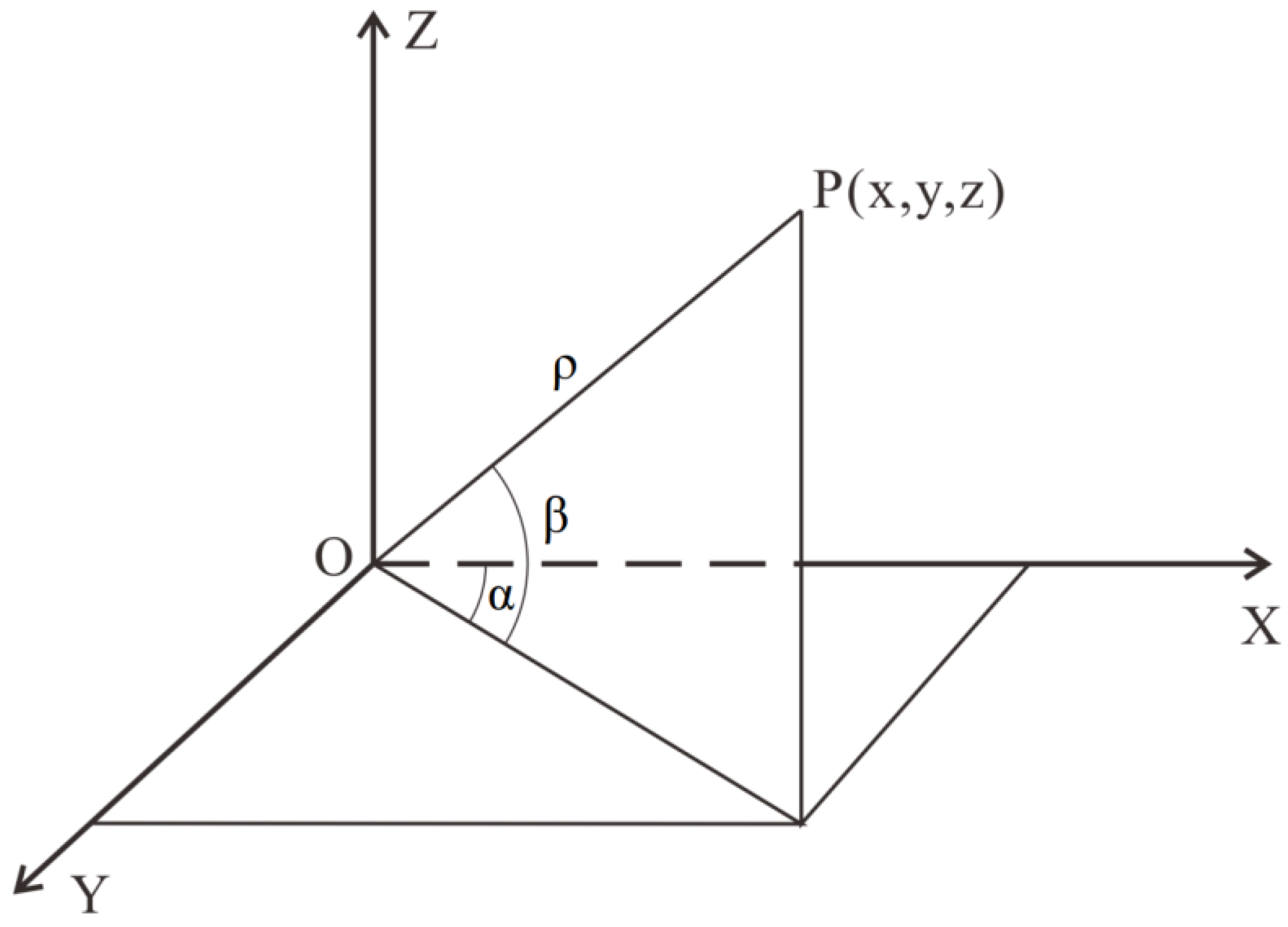
The laser pulse is reflected to the scanner by the objects in its path. The scanner sensor receives and records the time interval from the emission to the return of the laser pulse, from which the distance between the target point P and the scanner is calculated. The distance ρ, horizontal angle α, and vertical angle β between the scanner and the target object are shown in Figure 2.
According to Equation (1), the spatial coordinates of the target point P are calculated based on the distance between the point and the laser scanner (ρ), the relative vertical angle (β), and the relative horizontal angle (α).
2.2. Pre-Processing
2.2.1. Point Cloud Registration
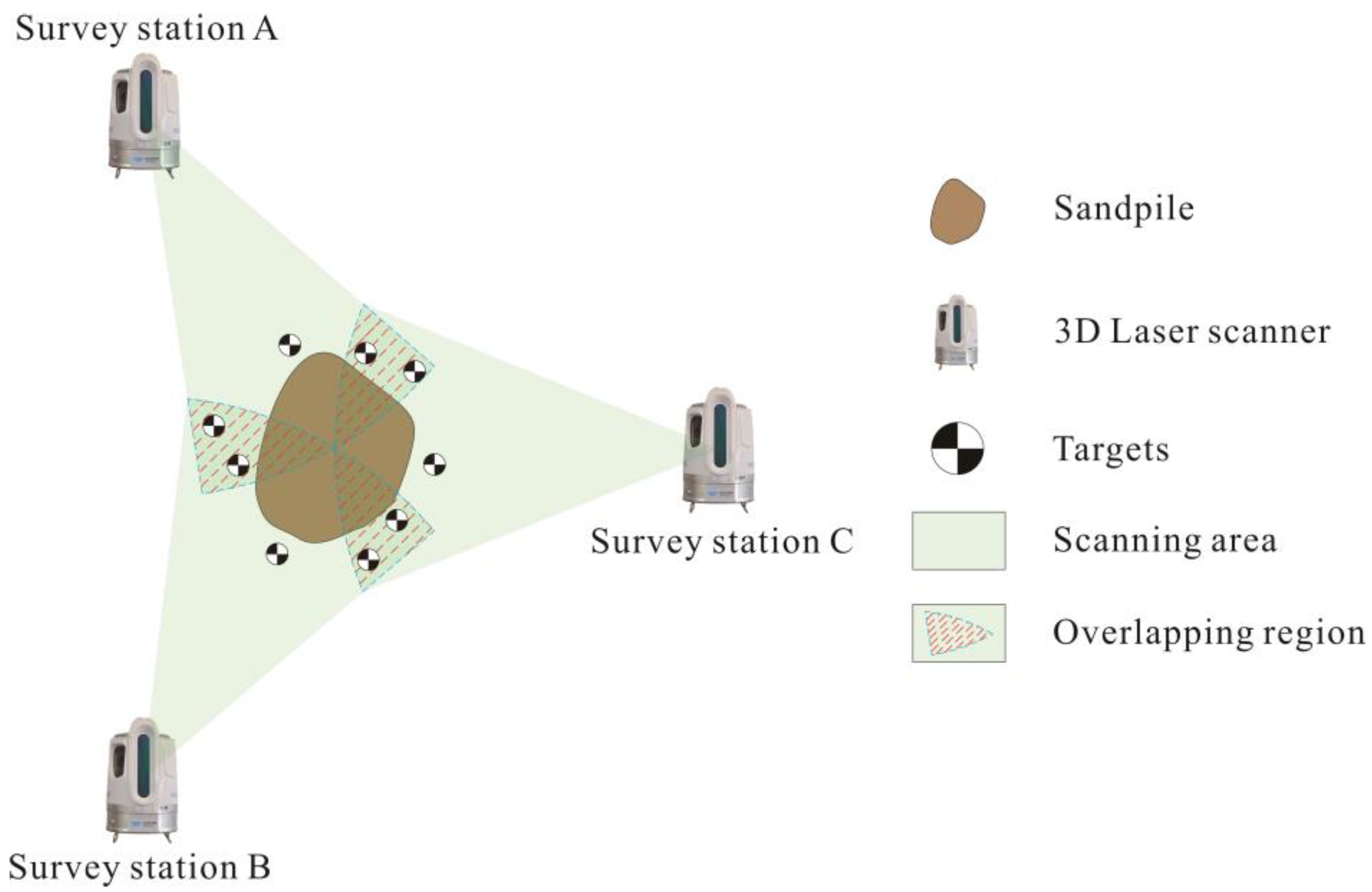
In practical works, obtaining complete point cloud data often requires multiple scans to collect point clouds of LEDs at different locations and angles. As shown in Figure 3, there is an overlap between the scanned areas of different stations, and the target points can be used to calibrate the conversion between adjacent scans and stitch the different point clouds together to obtain the overall surface of the LED. Moreover, these target points can convert the coordinate systems of the point clouds acquired by different stations into a unified specified coordinate system.
2.2.2. Point Cloud Denoising
Due to the influence of laser scanning equipment accuracy, the operator’s skills, the material of the measured object itself, and the environment surrounding the acquisition area, the acquired point clouds contain many interference points and invalid points, which reduce the fineness of the data. Efficient noise reduction of the scanned point cloud data is the key to ensuring the subsequent processing of the point cloud. Statistical filtering and radius filtering are two common methods for point cloud noise reduction.
The statistical filtering algorithm removes outliers from the point cloud by querying the distance between the points and the set of surrounding points, in the following process:
(1) Suppose the original point cloud dataset , the domain of each of these points is statistically analyzed, and the average distance from a point to the nearest k points in the domain is calculated, denoted as .
(2) Suppose the noise reduction point cloud data set , the statistical filtering algorithm envisages that in obeys a Gaussian distribution, defines μ as the mean and σ as the standard deviation, and has the following equations (Equations (2) and (3)):
(3) The points pi in the original point cloud dataset are judged, and if the average distance between pi and its domain is within , it is retained. Otherwise, it is removed as an outlier. In this algorithm, std values are set by humans, which controls the harshness of the screening. The appropriate std values are required to be selected carefully to obtain high-quality filtering results [25].
The idea of the radius filtering algorithm is: for a given threshold k, determine whether the number of points in the field of radius r of each point is smaller than the threshold k. If it is smaller, the point is considered a noise point and removed.
Furthermore, to improve the efficiency of point cloud processing, the point cloud is downsampled to reduce the number of point clouds and improve the quality of the point clouds, while ensuring the basic features and details of the scanned area.
2.3. Constructing a Complete Point Cloud
2.3.1. Fitting the Bottom Surface
Since the LED is connected to the ground, the 3D laser scan obtains a set of data that lacks a subface point cloud, is unconfined, and is not monolithic. Therefore, a bottom plane fitting was performed based on the initial point cloud of the LED and then its bottom plane was constructed. The essence of the plane fitting of point cloud data is to find a fitting plane to approximately replace the selected points, and the existing plane fitting algorithms are least squares, z-function fitting, the eigenvalue method, maximum likelihood estimation method, etc. [26]. This paper is mainly based on the least squares method for plane fitting to minimize the sum of the squares of the distances from all points in the point cloud to the fitting plane.
For the reference point cloud used to fit the bottom plane, a series of edge points were manually and uniformly selected and saved as a matrix of [x, y, z], according to these points for plane fitting. If the bottom plane of the sample object is nearly horizontal or approximately parallel to the XOY plane of the preset coordinate system at the time of scanning, the plane with the points of in the sample point cloud can be directly fitted, and is a range constant, determined according to the actual data. The specific principle of the bottom plane fitting is as follows:
Assume that the plane that is not the origin of the coordinates is:
The point cloud chosen to fit the plane is assumed to be the point set . The target best-fit plane is required to satisfy Equation (5).
where p (x, y, z) = 0, there is:
For Equation (6) to hold, it is necessary to find the partial derivatives of a, b, and c, and it is needed to satisfy that holds, finishing with:
Suppose that:
Then:
The coefficients of the plane equation are solved as:
The formula of the standard deviation of distance for accuracy assessment is shown in Equation (10):
where is the distance from the point to the fitted plane; is the plane distance from the point to the fitted plane.
2.3.2. Point Cloud 3D-to-2D Projection
In the previous step, the bottom plane of the LED was fitted. Then, the top point cloud of the LED was projected onto this fitted plane. As a result, the subface point cloud of the deposits can be constructed.
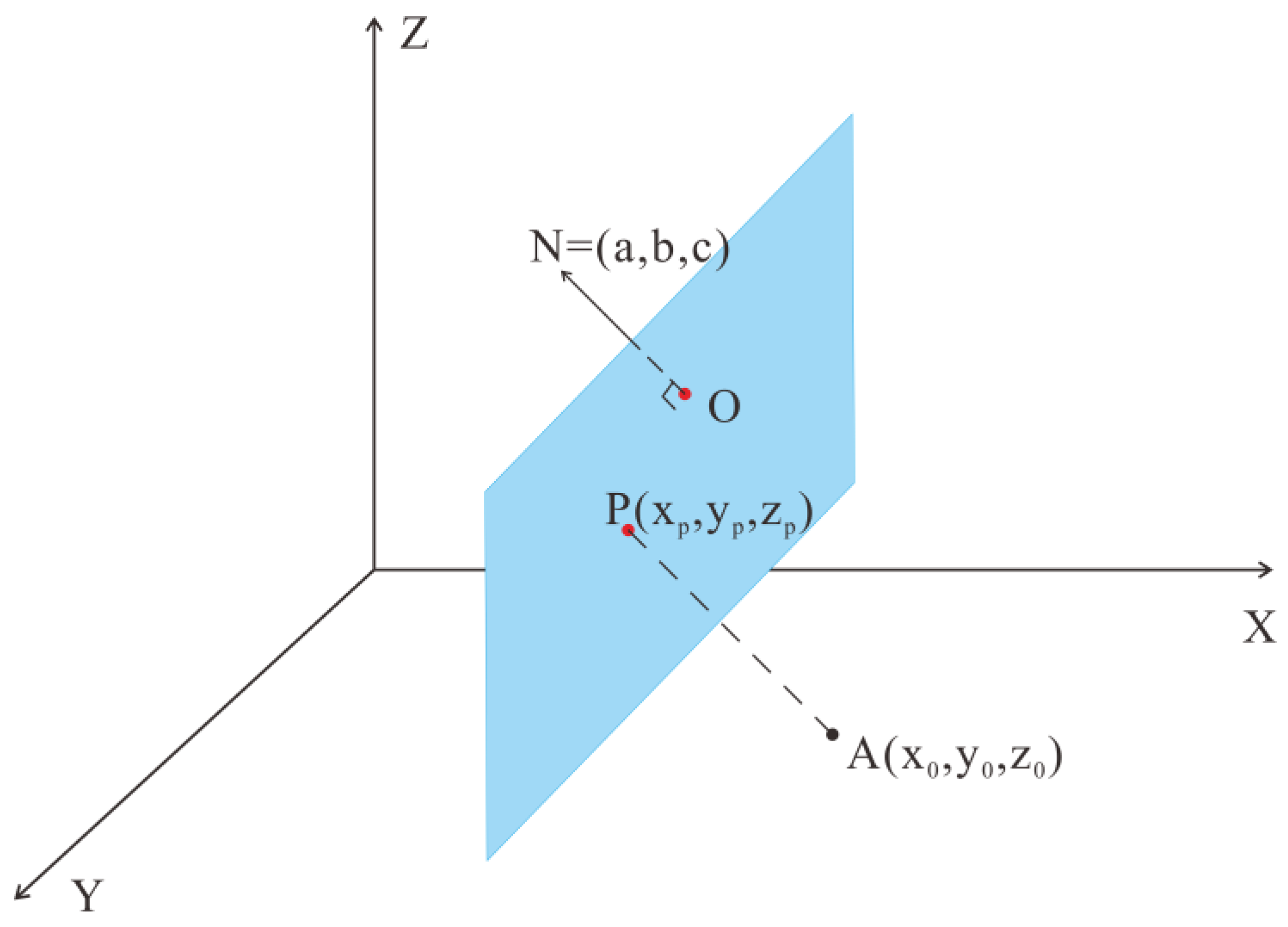
The 3D point to 2D plane projection is essentially finding the point in the plane that corresponds to the point outside the plane along the direction normal to the plane, as in Figure 4. The specific implementation plan can be written as Equation (4), and then the normal vector of this space plane is N = (a, b, c).
The equation of the line passing through a point outside the plane and perpendicular to the plane is:
Parametric equations:
The intersection of this line with the plane P is the desired point.
Then:
2.3.3. Point Cloud Stitching
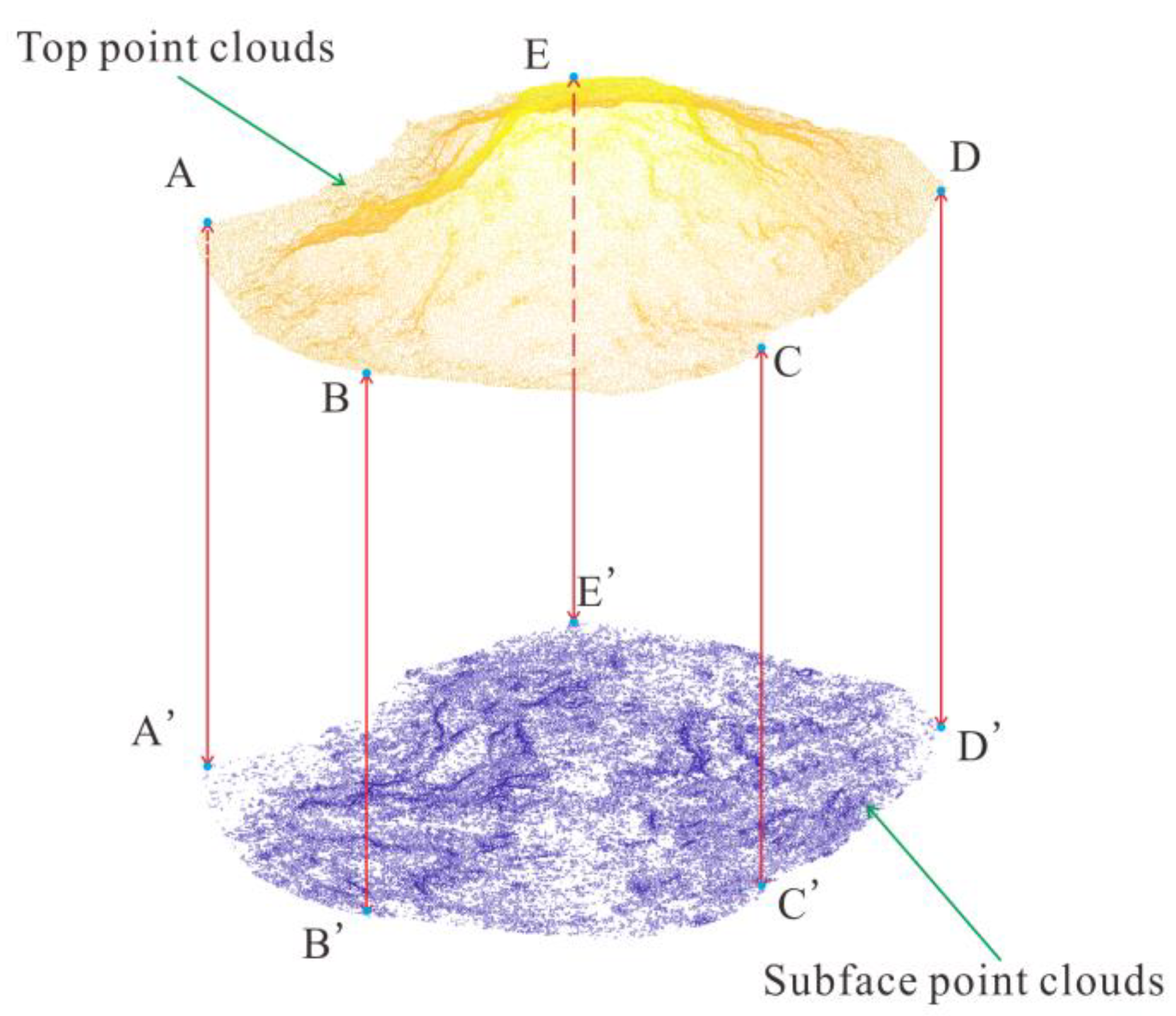
By stitching the obtained subface point clouds with the top point clouds, complete point cloud data of the LED can be obtained, and based on this, the subsequent volume calculation work can be performed, as shown in Figure 5.
2.4. Volume Calculation
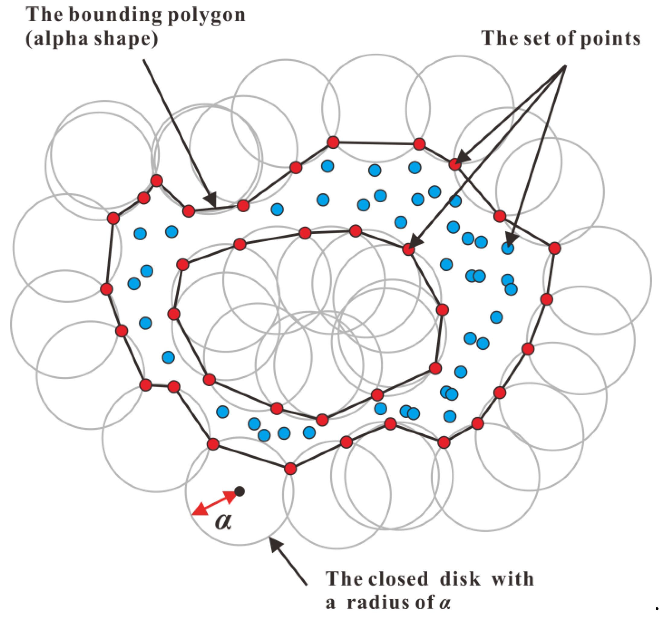
The alpha shape algorithm was proposed by Edelsbrunner [22,27] and was initially used for the construction of point set contours. To date, this algorithm has a wide range of applications for boundary identification of 2D and 3D points. The alpha shape algorithm can create a boundary surface for a set of 2D points or a boundary 3D body for a set of 3D points [19]. As shown in Figure 6, a 2D alpha shape is a bounding polygon determined jointly by the set of 2D points and the alpha radius α of a closed disk. Analogously, a 3D alpha shape is a 3D body determined by the set of spatial points P and the alpha radius parameter α of a ball that rolls outside the point set. Theoretically, when there exists a radius parameter, the alpha shape generates a three-dimensional convex package of the point set P. When the radius parameter α = 0, the alpha shape generates an empty set. When the radius parameter α takes appropriate values, the alpha shape generates concave places and holes with improved refinement. After converting the point cloud set into a closed polygon, the volume of the object can be estimated from the closed polygon.
3. Experiments
To evaluate the performance of the proposed LED volume determination method, two different sets of experiments are given in this paper, with point clouds from three soil mound models in the laboratory and LEDs in the field. Due to the very large volume and random shape of the field LED, the actual verification of the method accuracy for various LEDs is a difficult and time-consuming task. In this paper, a set of experiments were designed in the laboratory to measure the volume of three soil mound models with similar shaped LEDs, obtaining the real volume of the models by the wax seal suspension weighing method. Based on the satisfactory results of the model experiments, the practicality of the method was fully demonstrated and its performance was verified by comparing the volume determinations of the LEDs in the field with the volume values calculated by existing commercial software.
A Cartesian coordinate system was employed to represent the XYZ coordinates of point clouds in 3D space that were obtained by a terrestrial laser scanner for field work and handheld laser scanners for laboratory experiments. In the Cartesian coordinate system, the right-hand rule was introduced to describe the orientation of axes: the thumb points along the positive x-axis; the index finger indicates the positive y-axis; and the middle finger becomes the positive z-axis.
3.1. Validation Experiments in the Laboratory
3.1.1. Materials
The super-light clay and sand were mixed with a mass ratio of 1:5 to form the materials of the soil mound models, in which the sand material as aggregate and super-light clay played the role of adhesive, artificially assisting in forming the shape of the LED. The super-light clay (its composition was foaming powder, water, pulp, paste, etc.) is a new environment-friendly material that is non-toxic, tasteless, and non-irritating. This material has strong plasticity, easy to set, should not be cracked, etc.
3.1.2. Volume Determination by Handheld Laser Scanning
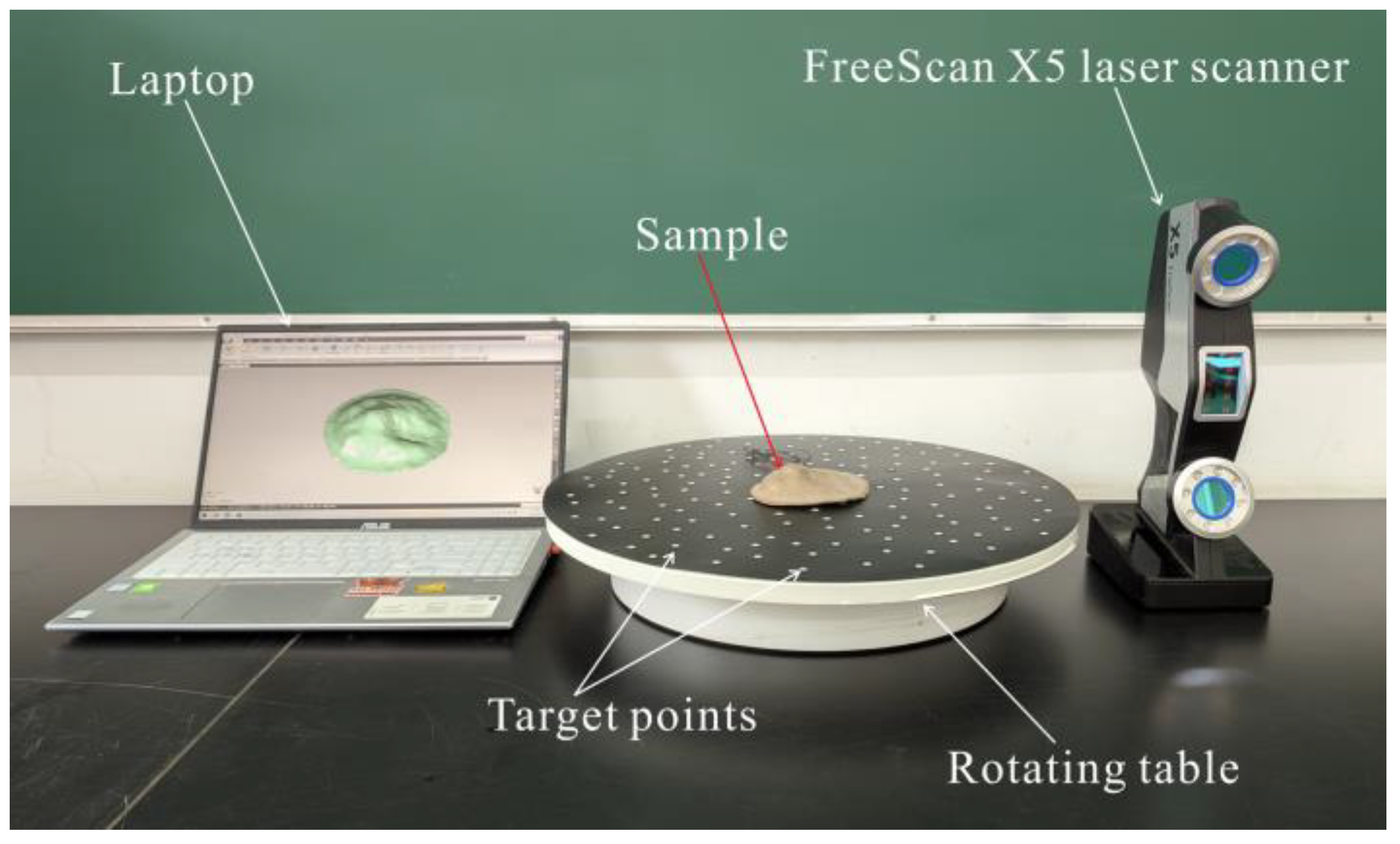
A handheld laser scanner (FreeScan X5) was used in this model experiment to obtain the point clouds of the three soil mound models. This portable laser scanner is suitable for small and complex-shaped specimens and met the measurement needs of this laboratory experiment. Its detailed performance and specifications are shown in Table 1.
The validation experiment was performed in the Rock Mechanics Laboratory, Faculty of Engineering, China University of Geosciences (Wuhan). The point cloud data acquisition system is shown in Figure 7. A handheld 3D laser scanner was used to acquire data, a laptop computer received and processed the data, and a table could be rotated 360° to change the scanning angle and positions of the laser scanner. Several reflective target points were required to assist the software in stitching together point clouds from different scanning orientations into a coherent point cloud of the scanned object. These target points were designed for laser sensor localization via triangulation during the task of point cloud registration. Theoretically, at least four non-collinear targets in the field of view needed to be aligned for each scanning [28]. In this study, at least five target points (with a diameter of 1 cm) were set up for each scanning to improve the measurement accuracy. In a word, the presence of target points allowed us to collect point clouds of soil mound models with higher accuracies. Finally, high-resolution point clouds of three soil mound models were obtained with 0.13, 0.15, and 0.15 mm point intervals for samples No. 1, No. 2, and No. 3, respectively.
Since the wax shell on the surface of the sample model after wax sealing is glossy and reflects light rather intensely, which makes the scanned point cloud data of poor quality, this experiment used the sample model before wax sealing as the object of the 3D laser scanning to obtain the point cloud data for subsequent processing and volume calculation. The three soil mound models, the models after wax sealing, and the acquired point cloud data are shown in Table 2.
After the point cloud data pre-processing, complete point cloud data were constructed as shown in Table 3. To balance the processing time, measuring resolution, and 3D reconstruction quality, the parameter α was set to 0.04 mm.
3.1.3. Wax Seal Suspension Weighing Method to Measure the Model Volume
To verify the volume calculated by the proposed method, the water displacement method was used to measure the same soil mound models in the laboratory. The soil mound model was firstly wax-sealed and then the true volume of the model was determined using an electronic scale suspension weighing method [29]. The experiments were performed by dipping a known mass of the sample model into melted wax to form a waterproof wax shell on its surface and to preserve its surface shape.
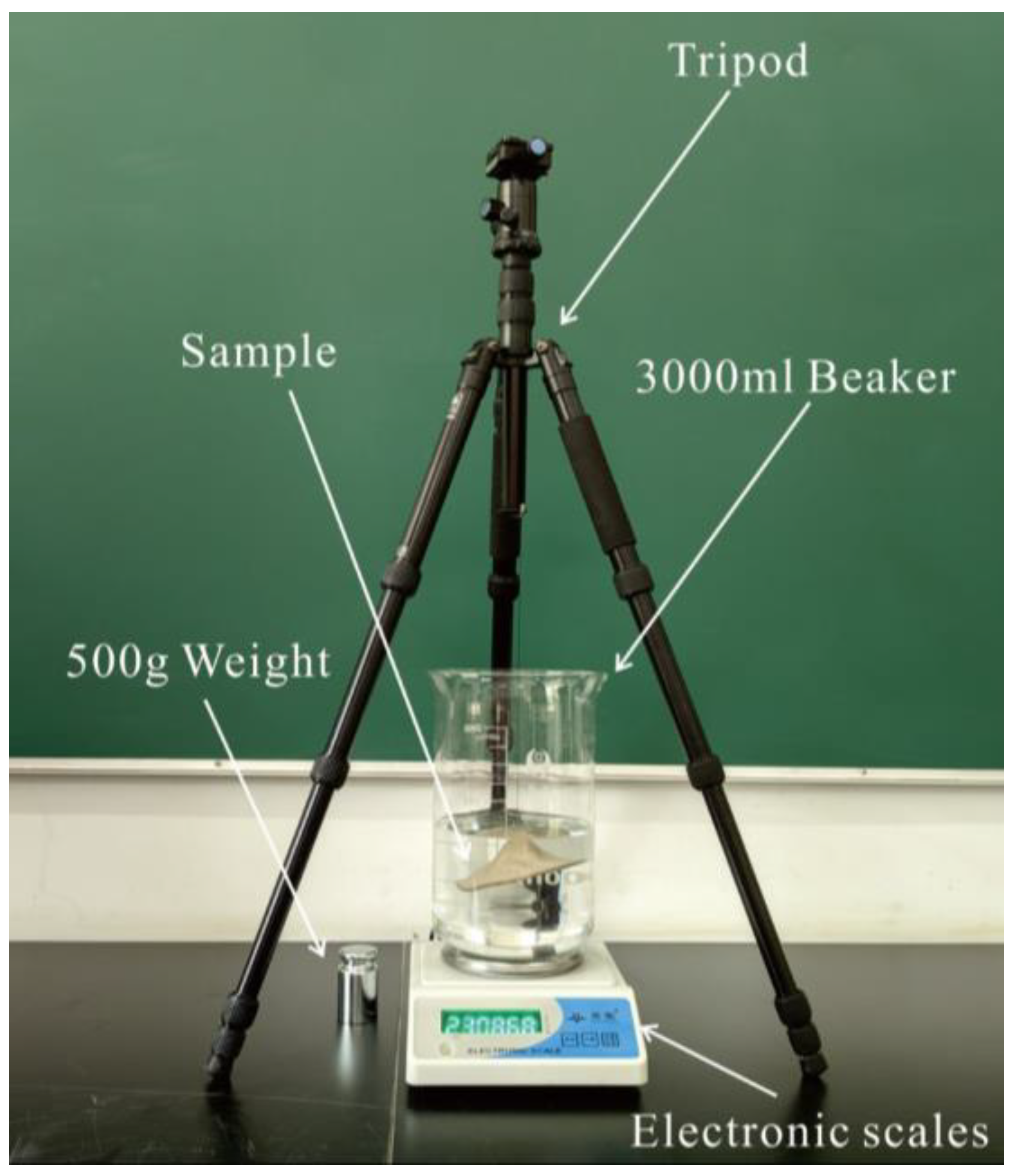
Figure 8 shows the schematic diagram of the experimental setup of the suspension weighing method, which was mainly composed of a tripod, an electronic scale (resolution: 0.01 g), a beaker (maximum capacity: 3000 mL), a thin string, a standard weight (weight: 500 g), wax-sealed sample models, water, etc. The detailed experimental methods were as follows:
- (1)
- Calibrate the electronic scale using the standard weight.
- (2)
- Use an electronic scale to measure the mass of the sample models before and after the wax immersion, noted as m and m0, respectively.
- (3)
- Fill the beaker with 1500 mL water, place it on the electronic scale, and read the scale after stabilization. The wax-sealed model is suspended from the tripod with a thin string and completely submerged in water, ensuring that the model does not come into contact with the bottom and side walls of the beaker, and then read the balance after stabilization, noted as m2.
According to Archimedes’ principle:
where F indicates the buoyancy of the soil mound model in the water; G indicates the gravity of the model discharging water; ρw indicates the density of the water under the experimental conditions and is specified as 0.98,997 g/cm3 in this paper; V indicates the volume of the model discharging water; g indicates the acceleration of gravity.
Under conditions of complete submersion:
where Vw is the volume of the model after wax sealing.
Sample model volume:
where m2 is the weight of the beaker, water, and wax-sealed soil mound model; m1 is the weight of beaker and water without soil mound models; and ρn is the density of the wax where 0.9 g/cm3 was used in this experiment.
3.1.4. Results and Analysis
After constructing complete point cloud data of the soil mound model, the volume results calculated by the alpha shape algorithm and the volume results obtained by the wax seal suspension weighing method are shown in Table 4.
The relative error of the volume calculation is calculated by the formula:
where is the true value of volume and is the measured value of volume.
The accuracy k of the volume calculation is related to the relative error:
The volume of the models obtained by the wax seal suspension weighing method was used as the control value, and it was found that the accuracy of the calculated volume of the scheme proposed in this paper was quite high, in which the relative error of No. 2 was only 1.69%, which was in line with the engineering reality and fully proved the reliability and repeatability of the scheme. An important source of error is that the bottom edge of the model is in more contact with the air when air-drying, and the edge cools and shrinks too fast relative to the center of the bottom surface. This causes warping, resulting in incomplete sampling of the bottom edge, as shown in the Figure 9 alpha shape image of No. 1. Based on the good test results in the laboratory, field experiments with LEDs were conducted for volume determination.
3.2. Real Engineering Deposit Volume Determination Experiment
3.2.1. General Situation of Loose Engineering Deposits
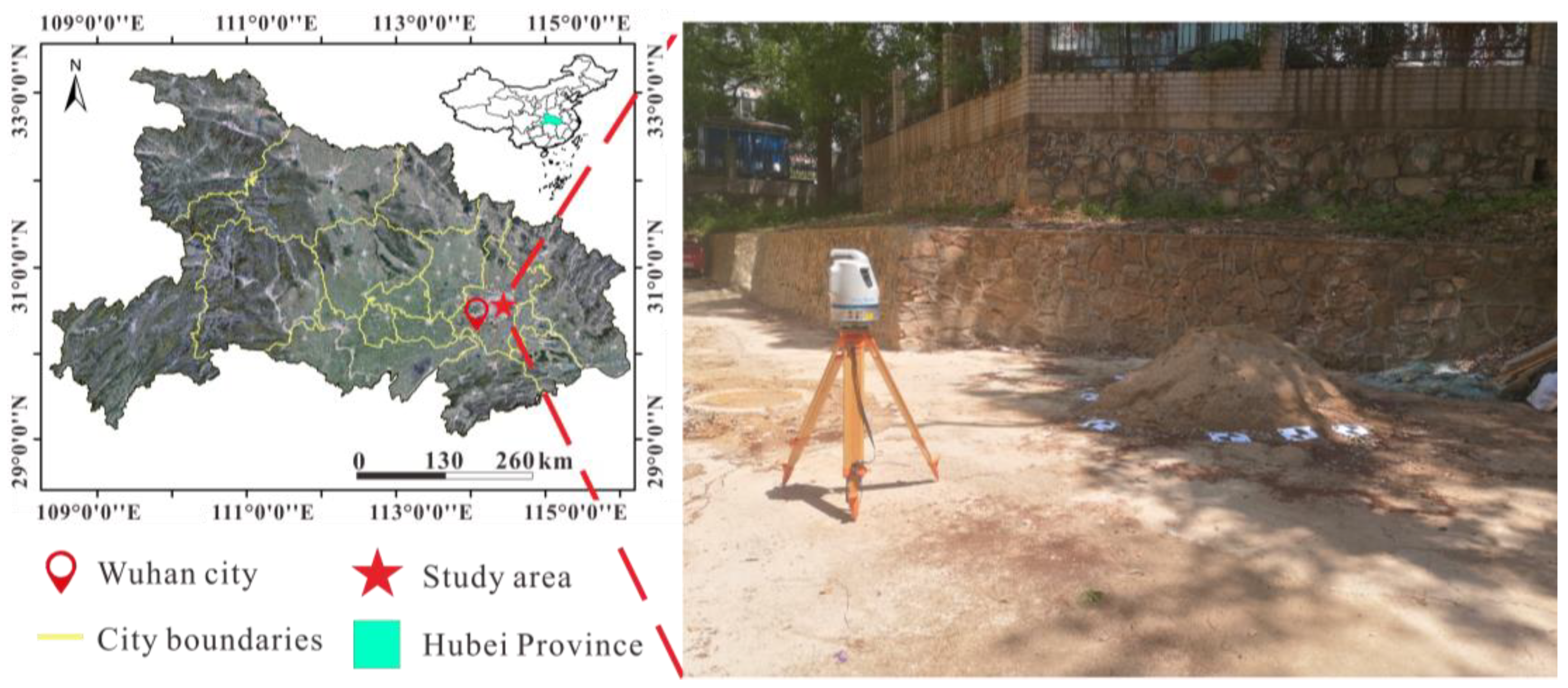
The field experimental study area for LED volume determination was located on the west campus of China University of Geosciences (Wuhan), and the experimental object was an engineering building sand deposit, hereafter referred to as the sand deposit, which was located on a flat surface, as shown in Figure 9.
3.2.2. Data Acquisition
An Optech Polaris LR 3D laser scanner was employed to capture the dense point clouds of the sand deposit, and the detailed performances and specifications are summarized in Table 5.
To ensure the accuracy of the data and the adequacy of the data volume, and also considering the size of the task and accessible space, the scanning distance between the laser scanner and sand deposit was specified as 3~5 m. Three workstations were set up around the sand deposit to obtain a 360° panoramic view of the sand deposit, and seven targets were arranged along the edge of the sand deposit. These seven targets were used to register the point clouds from three workstations into the same coordinate system (point cloud registration) to produce the complete point clouds of the whole sand deposit, based on which the volume calculation was then conducted. When the scanning work was completed, the built-in camera automatically collected images to generate the color information of the scanning area.
3.2.3. Volume Determination Results
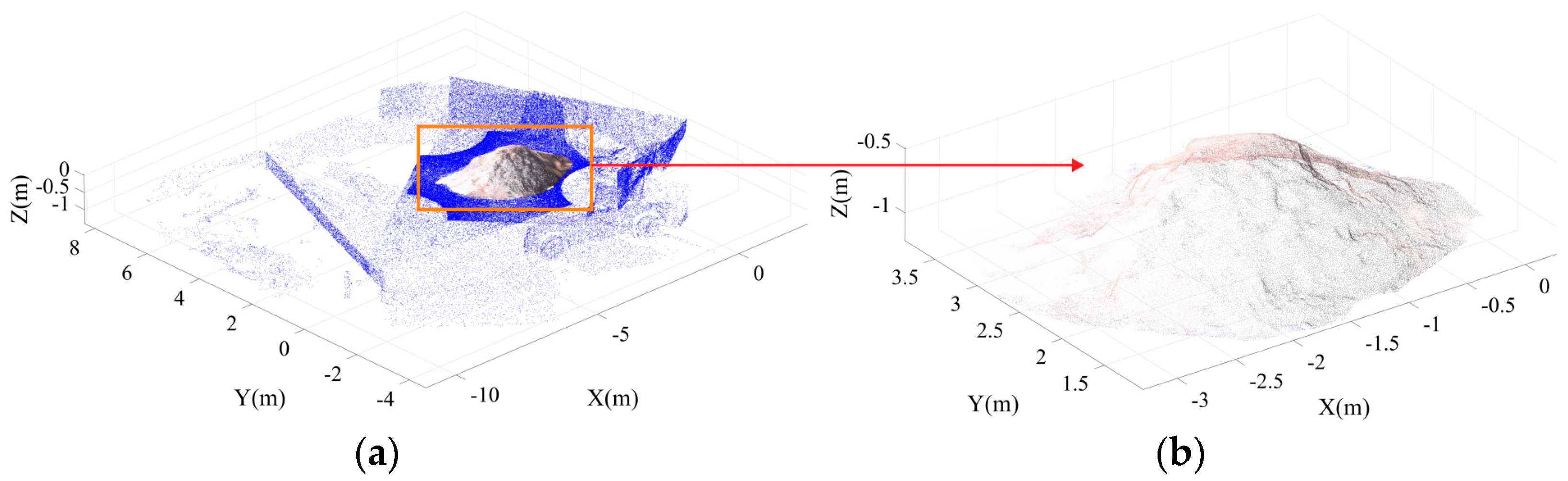
Figure 10a shows the point cloud data after the coordinate system assignment and data registration. It can be seen that the scanned point cloud data were massive and redundant, including the surrounding trees, walls, the ground far away from the sand deposit, etc. These were invalid points for the volume calculation of the deposit data, and the number of points reached 108,512,679 with a point interval of 12.5 mm, which would greatly reduce the post-processing efficiency. Figure 10b shows the point cloud data of the sand deposit after denoising and downsampling the data; the number of point clouds was 74,551 which is moderate, and it can be seen that the features of the sand deposit were also relatively fine.
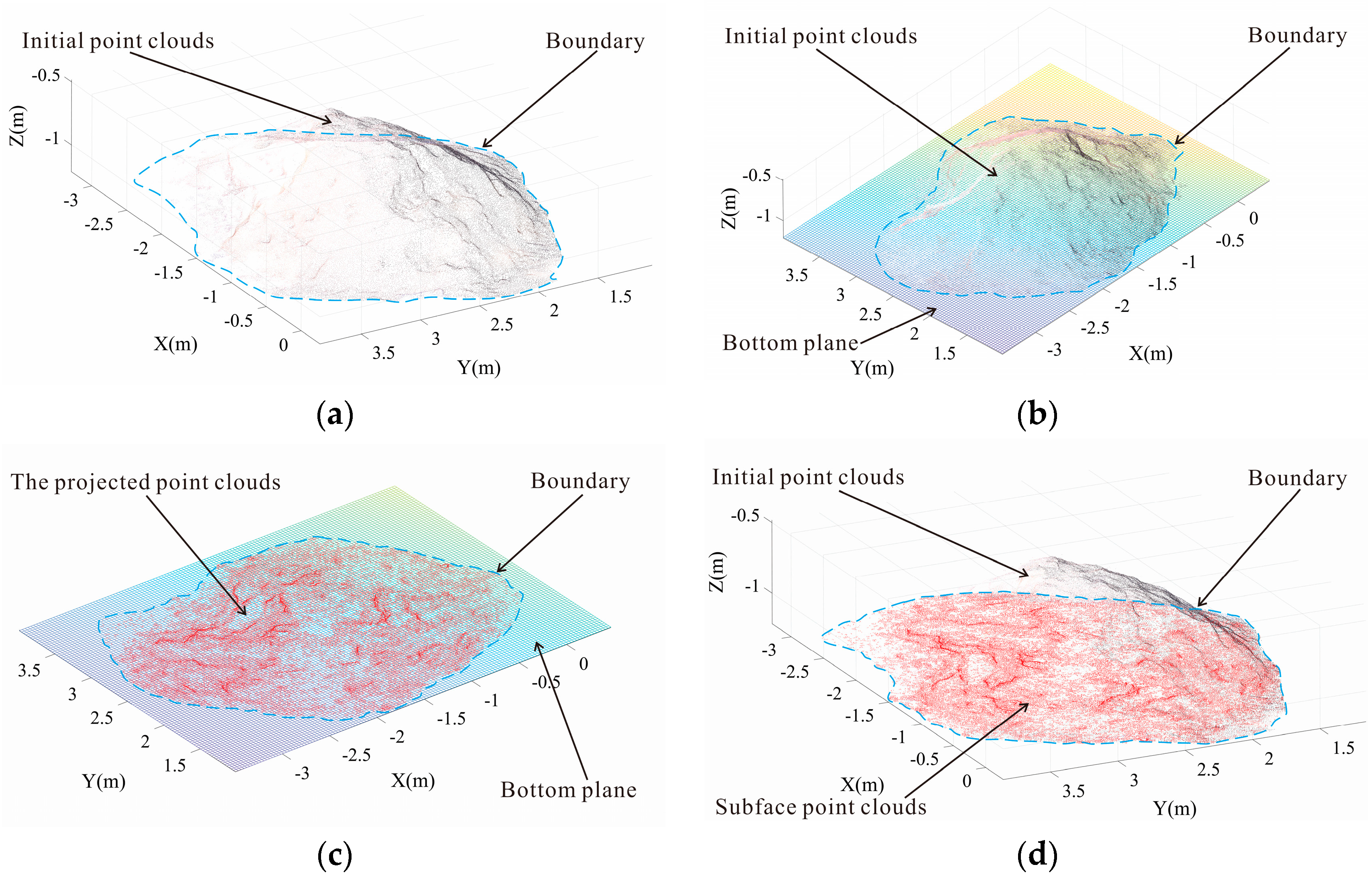
Assuming that the bottom surface of the sand deposit was approximately flat, Figure 11 shows the flow chart of the complete point cloud data construction. Figure 11a indicates the data without a bottom point cloud, unconfined and non-integral. Figure 11b indicates that the bottom plane is well-fitted and can represent the actual bottom surface of the sand deposit. Figure 11c indicates the effect of projecting the point cloud data to the fitted plane. Figure 11d indicates the final formed 3D complete point cloud data, which have the characteristics of good closure, good integrity, and high accuracy, and are very representative of the sand deposit.
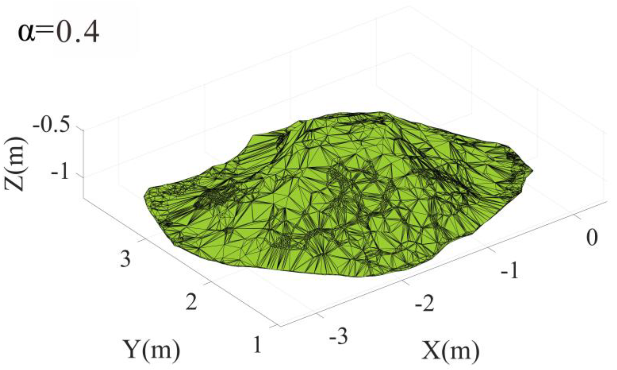
The selected parameter α = 0.4 m, as shown in Figure 12, was relatively fine for the three-dimensional reconstruction of the sand deposit, with detail reduction, a better expression effect, and more representativeness. The alpha shape algorithm volume calculation result was 1.847 m3, and the real value of 1.764 m3 showed a relative error of 4.71%, indicating a high accuracy and following the actual needs of the engineering.
4. Discussions
Starting from a point cloud obtained by scanning often lacks bottom surface point cloud data, so in this paper, the 3D point cloud was projected to the 2D plane by bottom plane fitting. Table 3 and Figure 11 show that the subface points obtained by this method can well determine the bottom plane boundary of the LED when the bottom surface is nearly flat, and the complete point clouds constructed have good representativeness for the LED. However, this proposed method does not apply to the case where the morphological characteristics of LEDs are large at the top and small at the bottom, because when the bottom surface is not the largest plane, the bottom point cloud data obtained from the point cloud projection onto the bottom plane cannot represent its true subface, and the bottom boundary cannot be determined.
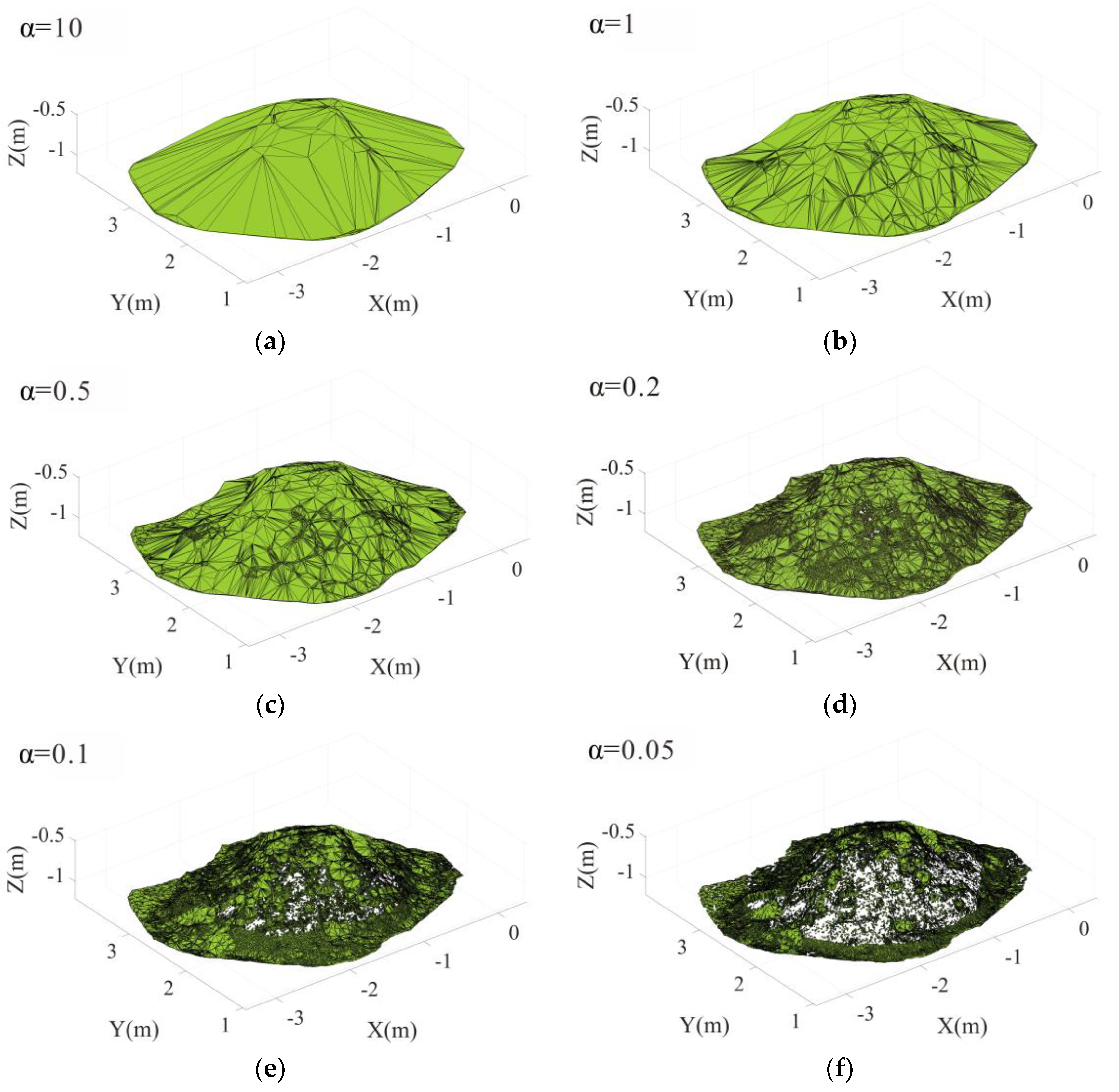
In the process of 3D reconstruction and volume calculation of the LED using the alpha shape algorithm, different parameters α can construct different spatial morphological features of the LED. As an example, Figure 13a–f shows the effect of alpha shape on the 3D modeling of the sand deposit when the parameters α are set to 10, 1, 0.5, 0.2, 0.1, and 0.05 m, respectively.
Meanwhile, in this paper, the volume results were calculated using the software Geomagic as the real value for the reference. In the Geomagic software, noise reduction was set as auto, and the small components were deleted during model building. Additionally, the maximum number of edges (holes) was specified as 20, and other options were set to default. To determine the appropriate parameter α, more α values (10, 1, 0.9, 0.8, 0.7, 0.6, 0.5, 0.4, 0.3, 0.2, 0.1, and 0.05 m) were considered to reconstruct the 3D models of soil mounds, and the corresponding volume results of the proposed algorithm with different parameters α are shown in Table 6.
As shown in Figure 13, when the parameter α = 10 m, the radius of the sphere is too large and the structure of the sand deposit is highly integrated, the generated model is a convex packet composed of the outermost point cloud of the data, and this model cannot express the specific details of the sand deposit clearly and the effect is not satisfactory. At the same time, combined with Table 4, the volume calculation result is large, 2.400 m3, and the real value of 1.764 m3 shows a relative error of 36.1% and does not meet the requirements. When the parameter α = 0.1 m, the radius of the sphere is too small, and it cannot find enough points to establish the boundary 3D body. The reconstruction result is incomplete, and there are more holes and defects. Meanwhile, combined with Table 6, the volume calculation result is small this time, 0.301 m3, and the relative error with the real value of 1.764 m3 is 82.9%, which does not meet the requirements. When the parameter α = 0.4 m is moderate, the 3D reconstruction model is finer and representative, and the corresponding volume calculation accuracy reaches 95.29%.
The selection of an appropriate parameter α highly depends on the geometry of the scanned object and measuring resolution. When the objects have complex shapes and surface contours, α is supposed to be set to a smaller value than the simple-shaped objects. In this study, both the soil samples in the laboratory and the sand deposits in the field site were characterized as mound-shaped, and therefore the geometry had a limited influence on the selection of the appropriate α for these two cases. On the other hand, the point interval is closely related to the measuring resolution. If there is a large point interval for the point cloud, correspondingly, a large α is supposed to be chosen for the 3D reconstruction. In this study, the point clouds of three soil mound models were collected using the handheld laser scanner with an approximate resolution of mm (0.13, 0.15, and 0.15 mm point intervals for samples No. 1, No. 2, and No. 3, respectively); while the terrestrial laser scanner was used to collect the point clouds of the sand deposits with a point interval of m (point interval ≈ 12.5 mm). Therefore, this is the major reason why the parameter α in the laboratory experiments (0.04 mm) was far less than the one described for the field experiments (0.4 m). A pre-determined α value may be specified to allow the comparison of the sizes and shape/surface contours of the reconstructed point clouds.
5. Conclusions
This paper proposes a new method to automatically determine the volume of LEDs using point clouds collected by terrestrial laser scanning equipment. Starting from the problem of lacking bottom surface point cloud data when scanning the LED, a plane fitting, point cloud projection method was used to combine the subface point cloud with the initial point cloud to form complete point cloud data with good representativeness for LEDs. The alpha shape algorithm was used to calculate and analyze the volume values of the deposits under different parameters and the fineness of the constructed 3D body, which is a simple and efficient method with applicability to general LEDs.
The reliability and reproducibility of this scheme were confirmed by the experiments conducted using the soil mound models in the laboratory, where the minimum error of volume determination reached 1.69%. The experiments on the field determination of the volume of sand deposit showed that the average accuracy of the method to extract the volume exceeded 95.29%, which verified the practicality of this scheme in practice. Also, the method can be applied to agriculture, such as for the automatic inventory calculation of grain deposits, the facilitation of scientific storage and transportation management, and the rationalization of production schedules, and other aspects of engineering practices.
The proposed method is not applicable to cases where the morphological characteristics of the LED are large at the top and small at the bottom. At the same time, to further deepen the universality of the proposed method, future study needs to solve the problem of how to determine the bottom boundary and improve its accuracy when the LED is located on uneven and undulating ground.
Author Contributions
Conceptualization, Y.G. and B.L.; methodology, Y.G. and J.Z.; software, J.Z., Y.G., Q.C., Z.W., G.L. and L.L.; validation, J.Z. and Y.G.; formal analysis, J.Z., Y.G. and Q.C.; investigation, J.Z. and Y.G.; resources, Y.G. and B.L.; data curation, J.Z. and B.L.; writing—original draft preparation, J.Z., B.L., G.L. and Y.G.; writing—review and editing, B.L., Y.G. and L.L.; visualization, J.Z., B.L. and Y.G.; supervision, B.L. and Y.G.; project administration, B.L. and Y.G.; funding acquisition, B.L. and Y.G. All authors have read and agreed to the published version of the manuscript.
Funding
This research was funded by the National Natural Science Foundation of China (No. 42077264), the Young Top-notch Talent Cultivation Program of Hubei Province (No. 20230550033), and the Scientific Research Project of China Three Gorges Group Co., Ltd. (No. JG/19056J).
Data Availability Statement
The data and materials that support the findings of this study are available from the corresponding author, Yunfeng Ge, upon reasonable request.
Acknowledgments
We thank the editors and anonymous reviewers for their useful comments.
Conflicts of Interest
The authors declare no conflict of interest.
References
- Kim, Y.H.; Shin, S.S.; Lee, H.K.; Park, E.S. Field applicability of earthwork volume calculations using unmanned aerial vehicle. Sustainability 2022, 14, 9331. [Google Scholar] [CrossRef]
- Bügler, M.; Borrmann, A.; Ogunmakin, G.; Vela, P.A.; Teizer, J. Fusion of photogrammetry and video analysis for productivity assessment of earthwork processes. Comput. Aided Civ. Infrastruct. Eng. 2017, 32, 107–123. [Google Scholar] [CrossRef]
- Yang, X.; Huang, Y.; Zhang, Q. Automatic stockpile extraction and measurement using 3D point cloud and multi-scale directional curvature. Remote Sens. 2020, 12, 960. [Google Scholar] [CrossRef]
- Matsimbe, J.; Mdolo, W.; Kapachika, C.; Musonda, I.; Dinka, M. Comparative utilization of drone technology vs. traditional methods in open pit stockpile volumetric computation: A case of njuli quarry, Malawi. Front. Built Environ. 2022, 8, 1037487. [Google Scholar] [CrossRef]
- Zhang, Q. A new approach for fast calculation of sloped terrace earthwork based on GIS in the hilly regions. In Computer and Computing Technologies in Agriculture VI: 6th IFIP WG 5.14 International Conference, CCTA 2012, Zhangjiajie, China, 19–21 October 2012; Revised Selected Papers, Part II 6; Springer: Berlin/Heidelberg, Germany, 2013; pp. 464–471. [Google Scholar]
- Du, J.C.; Teng, H.C. 3D laser scanning and GPS technology for landslide earthwork volume estimation. Autom. Constr. 2007, 16, 657–663. [Google Scholar] [CrossRef]
- Jaboyedoff, M.; Carrea, D.; Derron, M.-H.; Oppikofer, T.; Penna, I.M.; Rudaz, B. A review of methods used to estimate initial landslide failure surface depths and volumes. Eng. Geol. 2020, 267, 105478. [Google Scholar] [CrossRef]
- Scheidegger, A.E. On the prediction of the reach and velocity of catastrophic landslides. Rock Mech. 1973, 5, 231–236. [Google Scholar] [CrossRef]
- Zhou, T.; Ge, Y.; Zheng, M.; Xia, D.; Hu, Y.; Zhong, P.; Wen, L. Study on volume calculation method of landslides in Valles Marineris. Saf. Environ. Eng. 2017, 4, 34–42. [Google Scholar]
- Guo, J.R.; Wang, Y.L.; Yu, L. Resolution of object surface and method of surface areas and volumes calculation. J. Shandong Univ. Technol. 2014, 28, 73–78. [Google Scholar]
- Su, C.Y.; Sui, L.C. Rapid measurement of earthwork based on three-dimensional laser scanning technology. Surv. Mapp. Technol. Equip. 2014, 2, 49–51+8. [Google Scholar]
- Xiang, D.; Wang, Z.M.; Zhao, J.H. Comparative analysis of RTK and TPS in the measurement of mineral bulk volume. Urban Surv. 2002, 4, 61–62+37. [Google Scholar]
- McEwen, A.S. Mobility of large rock avalanches: Evidence from Valles Marineris, Mars. Geology 1989, 17, 1111–1114. [Google Scholar] [CrossRef]
- Ge, Y.; Cao, B.; Chen, Q.; Wang, Y. Rock Joints Detection from 3D Point Clouds Based on Color Space. Q. J. Eng. Geol. Hydrogeol. 2023, 56, qjegh2023-012. [Google Scholar] [CrossRef]
- Ge, Y.; Tang, H.; Xia, D.; Wang, L.; Zhao, B.; Teaway, J.W.; Zhou, T. Automated measurements of discontinuity geometric properties from a 3D-point cloud based on a modified region growing algorithm. Eng. Geol. 2018, 242, 44–54. [Google Scholar] [CrossRef]
- Ge, Y.; Liu, J.; Zhang, X.; Tang, H.; Xia, X. Automated Detection and Characterization of Cracks on Concrete Using Laser Scanning. J. Infrastruct. Syst. 2023, 29, 04023005. [Google Scholar] [CrossRef]
- Yin, Y.; Antonio, J. Application of 3D laser scanning technology for image data processing in the protection of ancient building sites through deep learning. Image Vis. Comput. 2020, 102, 103969. [Google Scholar] [CrossRef]
- Liu, J.; Xu, D.; Hyyppa, J.; Liang, Y. A Survey of applications with combined BIM and 3D laser scanning in the life cycle of buildings. IEEE J. Sel. Top. Appl. Earth Obs. Remote Sens. 2021, 14, 5627–5637. [Google Scholar] [CrossRef]
- Ge, Y.; Lin, Z.; Tang, H.; Zhong, P.; Cao, B. Measurement of particle size of loose accumulation based on alpha shapes (AS) and hill climbing-region growing (HC-RG) algorithms. Sensors 2020, 20, 883. [Google Scholar] [CrossRef]
- Lai, Y.H.; Yu, J.H.; Gu, Y. Volume Estimation of Harbor Engineering Objects Using Underwater Three-Dimensional Sonar. In Proceedings of the 2022 8th International Conference on Control, Automation and Robotics (ICCAR), Xiamen, China, 8–10 April 2022; pp. 49–54. [Google Scholar]
- Huising, E.J.; Gomes Pereira, L.M. Errors and accuracy estimates of laser data acquired by various laser scanning systems for topographic applications. ISPRS J. Photogramm. Remote Sens. 1998, 53, 245–261. [Google Scholar] [CrossRef]
- Edelsbrunner, H.; Mücke, E.P. Three-dimensional alpha shapes. ACM Trans. Graph. 1994, 13, 43–72. [Google Scholar] [CrossRef]
- Akkiraju, N.; Edelsbrunner, H.; Facello, M.; Fu, P.; Mucke, E.P.; Varela, C. Alpha shapes: Definition and software. In Proceedings of the 1st International Computational Geometry Software Workshop, Minneapolis, MN, USA, 11 September 1995; pp. 63–66. [Google Scholar]
- Pfeifer, N.; Briese, C. Laser scanning–principles and applications. In Proceedings of the Geosiberia 2007—International Exhibition and Scientific Congress, Novosibirsk, Russia, 25 April 2007; p. cp-59. [Google Scholar]
- Lu, D.D.; Zou, J.G. Comparative research on denoising algorithms of 3D laser point cloud. Surv. Mapp. Bull. 2019, 52, 102–105. [Google Scholar]
- Wang, C.; Tanahashi, H.; Hirayu, H.; Niwa, Y.; Yamamoto, K. Comparison of local plane fitting methods for range data. In Proceedings of the 2001 IEEE Computer Society Conference on Computer Vision and Pattern Recognition, CVPR 2001, Kauai, HI, USA, 8–14 December 2001; IEEE: Piscataway, NJ, USA, 2001; Volume 1, p. I-I. [Google Scholar]
- Edelsbrunner, H.; Kirkpatrick, D.; Seidel, R. On the shape of a set of points in the plane. IEEE Trans. Inf. Theory 1983, 29, 551–559. [Google Scholar] [CrossRef]
- Koessler, L.; Cecchin, T.; Caspary, O.; Benhadid, A.; Vespignani, H.; Maillard, L. EEG–MRI Co-registration and sensor labeling using a 3D laser scanner. Ann. Biomed. Eng. 2011, 39, 983–995. [Google Scholar] [CrossRef] [PubMed]
- Zhao, T.Y.; Zhang, H.Y.; Yan, G.S.; Zhang, Y.X. Application of electronic balance in the paraffin-coated method to determining soil density. Geotech. Investig. Surv. 2009, 5, 6–9. [Google Scholar]
Figure 1.
Flow chart of the main methodology.

Figure 2.
Schematic diagram of the key parameters of the 3D laser scanning determination.

Figure 3.
3D laser scanning technology working schematic.

Figure 4.
Projection of 3D point to a 2D plane.

Figure 5.
Point cloud stitching diagram (points A, B, C, D, and E are the typical points on the boundary of the top point clouds, correspondingly, points A’, B’, C’, D’, and E’ are the typical points on the boundary of the generated subface point clouds).
Figure 5.
Point cloud stitching diagram (points A, B, C, D, and E are the typical points on the boundary of the top point clouds, correspondingly, points A’, B’, C’, D’, and E’ are the typical points on the boundary of the generated subface point clouds).

Figure 6.
Schematic diagram of 2D alpha shape algorithm.

Figure 7.
Schematic diagram of the point cloud acquisition system.

Figure 8.
Schematic diagram of the experimental setup of the suspension weighing method.

Figure 9.
Overview of the field experiment area.

Figure 10.
Point cloud denoising: (a) the raw point cloud (blue points are noise data); (b) the denoised point cloud.
Figure 10.
Point cloud denoising: (a) the raw point cloud (blue points are noise data); (b) the denoised point cloud.

Figure 11.
Point clouds of sand deposits at different steps: (a) raw point cloud of the sand deposits without the bottom point cloud; (b) fitting of the bottom plane; (c) projection of the raw point cloud onto the fitted bottom plane; (d) complete point clouds of the sand deposits.
Figure 11.
Point clouds of sand deposits at different steps: (a) raw point cloud of the sand deposits without the bottom point cloud; (b) fitting of the bottom plane; (c) projection of the raw point cloud onto the fitted bottom plane; (d) complete point clouds of the sand deposits.

Figure 12.
Sand deposit 3D alpha shape reconstruction result (α = 0.4 m).

Figure 13.
Variation of the 3D reconstruction of the sand deposits with different parameters α: (a) α = 10 m, (b) α = 1 m, (c) α = 0.5 m, (d) α = 0.2 m, (e) α = 0.1 m, and (f) α = 0.05 m.
Figure 13.
Variation of the 3D reconstruction of the sand deposits with different parameters α: (a) α = 10 m, (b) α = 1 m, (c) α = 0.5 m, (d) α = 0.2 m, (e) α = 0.1 m, and (f) α = 0.05 m.


Table 1.
Specifications of the handheld 3D laser scanner FreeScan X5.
| Parameter | Specifications |
|---|---|
| Dimentions | 130 × 90 × 310 mm |
| Weight | 0.8 kg (net weight for the laser scanner) |
| Scan speed | 350,000 points/s |
| Precision | 0.030 mm |
| Working distance | 300 mm |
| Scan region | 100–8000 mm |
| Maximum resolution | 0.050 mm |
Table 2.
Comparison of the morphology of the three models before and after wax sealing and in 3D point cloud images.
Table 2.
Comparison of the morphology of the three models before and after wax sealing and in 3D point cloud images.
| Sample ID | Pre-Wax-Seal | Post-Wax-Seal | Point Cloud |
|---|---|---|---|
| 1 |  |  |  |
| 2 |  |  |  |
| 3 |  |  |  |
Table 3.
Construction of complete point cloud data and alpha shape 3D reconstruction schematic.
| Sample ID | Point Cloud without Subface | Complete Point Cloud | Alpha Shape |
|---|---|---|---|
| 1 |  |  |  |
| 2 |  |  |  |
| 3 |  |  |  |
Table 4.
Volume determination results and comparisons.
| Sample ID | Alpha Shape Algorithm α = 0.04 | Wax Seal Suspension Weighing Method | Difference | Relative Errors |
|---|---|---|---|---|
| Volume (m3) | ||||
| 1 | 79.403 | 81.273 | −1.87 | 2.30% |
| 2 | 95.995 | 97.649 | −1.654 | 1.69% |
| 3 | 130.110 | 137.774 | −7.664 | 5.56% |
Table 5.
Specifications of the Optech Polaris LR laser scanner.
| Parameter | Specifications |
|---|---|
| Range measurement principle | Pulsed |
| Wavelength | 1550 nm (near infrared) |
| Max. field of view (horizontal) | 360° |
| Max. field of view (vertical) | 120° (−45 to +75°) |
| Precision, single shot (1 sigma) | 4 mm @ 100 m |
| Range Resolution | 2 mm |
| Scan speed | 500,000 points/s |
| Scan distance | 1.5–2000 m |
Table 6.
Comparison of sand deposit volume between the different methods.
| Methods | The Algorithm Proposed in This Study | Geomagic | |||||||||||
|---|---|---|---|---|---|---|---|---|---|---|---|---|---|
| α (m) | 10 | 1 | 0.9 | 0.8 | 0.7 | 0.6 | 0.5 | 0.4 | 0.3 | 0.2 | 0.1 | 0.05 | — |
| V (m3) | 2.400 | 2.047 | 2.016 | 1.960 | 1.952 | 1.913 | 1.882 | 1.847 | 1.422 | 0.851 | 0.301 | 0.102 | 1.764 |
| Relative errors | 36.1% | 16.0% | 14.3% | 11.1% | 10.7% | 8.45% | 6.69% | 4.71% | 19.4% | 51.8% | 82.9% | 94.2% | 0 |
Disclaimer/Publisher’s Note: The statements, opinions and data contained in all publications are solely those of the individual author(s) and contributor(s) and not of MDPI and/or the editor(s). MDPI and/or the editor(s) disclaim responsibility for any injury to people or property resulting from any ideas, methods, instructions or products referred to in the content. |
© 2023 by the authors. Licensee MDPI, Basel, Switzerland. This article is an open access article distributed under the terms and conditions of the Creative Commons Attribution (CC BY) license (https://creativecommons.org/licenses/by/4.0/).
Share and Cite
MDPI and ACS Style
Lu, B.; Zhu, J.; Ge, Y.; Chen, Q.; Wen, Z.; Liu, G.; Li, L. Automated Determination of the Volume of Loose Engineering Deposits Using Terrestrial Laser Scanning. Remote Sens. 2023, 15, 4604. https://doi.org/10.3390/rs15184604
AMA Style
Lu B, Zhu J, Ge Y, Chen Q, Wen Z, Liu G, Li L. Automated Determination of the Volume of Loose Engineering Deposits Using Terrestrial Laser Scanning. Remote Sensing. 2023; 15(18):4604. https://doi.org/10.3390/rs15184604
Chicago/Turabian StyleLu, Bo, Jichen Zhu, Yunfeng Ge, Qian Chen, Zhongxu Wen, Geng Liu, and Liangquan Li. 2023. "Automated Determination of the Volume of Loose Engineering Deposits Using Terrestrial Laser Scanning" Remote Sensing 15, no. 18: 4604. https://doi.org/10.3390/rs15184604
Note that from the first issue of 2016, this journal uses article numbers instead of page numbers. See further details here.